Sparse Constrained Low Tensor Rank Representation Framework for Hyperspectral Unmixing

Abstract

Recently, non-negative tensor factorization (NTF) as a very powerful tool has attracted the attention of researchers. It is used in the unmixing of hyperspectral images (HSI) due to its excellent expression ability without any information loss when describing data. However, most of the existing unmixing methods based on NTF fail to fully explore the unique properties of data, for example, low rank, that exists in both the spectral and spatial domains. To explore this low-rank structure, in this paper we learn the different low-rank representations of HSI in the spectral, spatial and non-local similarity modes. Firstly, HSI is divided into many patches, and these patches are clustered multiple groups according to the similarity. Each similarity group can constitute a 4-D tensor, including two spatial modes, a spectral mode and a non-local similarity mode, which has strong low-rank properties. Secondly, a low-rank regularization with logarithmic function is designed and embedded in the NTF framework, which simulates the spatial, spectral and non-local similarity modes of these 4-D tensors. In addition, the sparsity of the abundance tensor is also integrated into the unmixing framework to improve the unmixing performance through the $L_{2,1}$ norm. Experiments on three real data sets illustrate the stability and effectiveness of our algorithm compared with five state-of-the-art methods.

1. Introduction

Hyperspectral remote sensing images are widely used in classification [1,2], target recognition [3], detection [4] and segmentation [5] tasks since they contain hundreds of spectral information bands. Unfortunately, hyperspectral images (HSI) generally have a low spatial resolution, and a large number of mixed pixels exist in the image, which hinders the application of remote sensing technology. To solve this problem, unmixing is used to extract all the pure spectra (i.e., endmember) in each pixel and the proportion (i.e., abundance) of each endmember [6,7]. In the current research, there are two main kinds of unmixing models. One is the linear mixed model (LMM) assuming that the pixels are linearly expressed by all endmembers in the image, and the other is the nonlinear mixed model, which assumes that there are multiple complex interactions among endmembers [8,9]. Since LMM is simple and easy to model, this paper only discusses the unmixing algorithm under the linear mixing assumption.

In recent years, the non-negative matrix factorization (NMF) framework has received extensive attention since its clear physical interpretability and strong ability of data representation among unmixing algorithms under the assumption of the LMM model. NMF aims at finding a set of bases that can express the data as accurately as possible and the expression coefficients of the data under the bases [10]. However, the NMF framework that regards unmixing as a blind source separation problem is non-convex problem with respect to two matrices obtained, which is greatly affected by the initial value and the solution is not stable enough [11]. Therefore, to improve the performance of unmixing, many regularizations are added to the NMF framework based on the prior knowledge about hyperspectral data, such as sparse regularization [12,13,14], smoothing regularization [15,16], non-local similarity regularization [17], manifold regularization [18], and low-rank regularization [19,20]. Hong et al. [21] embed the spectral variability dictionary learning into the linear NMF framework to make the endmembers more accurate. Unfortunately, the unmixing algorithm based on the NMF framework has a flaw, which destroys the integrity of the input data since the 3-D HSI is reshaped into a 2-D matrix. Recently, inspired by the success of non-negative tensor factorization (NTF), which regards HSI as a 3-D tensor without any information loss, a framework based on NTF framework has developed and shown superior performance in hyperspectral unmixing [22,23,24,25,26]. Regrettably, the existing unmixing methods based on NTF mostly focus on the similarity of abundance on the spatial domain, which are not conducive to fully exploring the internal similarity structure of data, such as non-local spatial similarity and information redundancy in the spectral direction.

To overcome the above issues, a new sparse-constrained low-rank tensor factorization (SCLT) framework is proposed for hyperspectral unmixing in this paper, which integrates a multi-mode low-rank learning regularization and a sparsity constraint by $L_{2,1}$ norm. Firstly, the hyperspectral data are divided into many patches with the same size. Then, all similar patches are clustered into the same group. Each similarity group can be regarded as a 4-D tensor, which has four modes, including two spatial modes in vertical and horizontal directions, a spectral mode and a non-local similarity mode. Since 4-D tensors are composed of multiple similar patches, all four modes have strong similar relationships. Therefore, a low-rank regularization is designed here to learn these strong similarities, which can express the multi-directional low-rank structure of HSI. In addition, based on prior knowledge, the abundance is sparse. To explore the sparse structure of the abundance tensor, the $L_{2,1}$ norm is introduced into the unmixing model to constrain the abundance tensor. Specifically, during each iteration, the sparse regularization is used to force the abundance tensor to remain sparse, and the low-rank regularization plays an important role in exploring the similarity relationship in the various modes of HSI. Since the proposed SCLT is a multi-variate problem, the alternative direction multiple method (ADMM) is utilized to optimize the objective function. For convenience, the contributions of this paper can be summarized as follows:

• A new sparsity-constrained low-rank tensor factorization model (SCLT) is proposed for unmixing, which aims at maintaining the low-rank spatial structure of the raw data and the sparsity of the abundance tensor in the iterative process.
• A regularization is designed to explore the low-rank structure of data, which can learn the low-rank representation of 4-D tensor containing similarity patches in spectral mode, spatial mode and non-local similarity mode.
• The sparsity constraint is embedded in the proposed model to explore the sparsity structure of the abundance tensor through the $L_{2,1}$ norm, which can improve the performance of unmixing.

The rest of this paper is organized as follows. Section 2 introduces some works related to NTF. The problem under the NTF unmixing framework is formulated in Section 3. Section 4 describes the method proposed in this paper in detail. Section 5 and Section 6 are the experimental analysis and conclusions, respectively.

2. Related Work

For hyperspectral mixed pixels, NMF has proved as a very effective method for unmixing. Under the LMM, the goal of NMF is to decompose a 3-D HSI reshaped into a 2-D matrix into two matrices, which are the endmember matrix and the abundance matrix. Specifically, each pixel in the hyperspectral data can be synthesized by the endmember matrix and its corresponding coefficients [27]. This model can accurately simulate a large number of mixed pixels, and the calculation is simple, convenient and easy to understand. However, for both the endmember matrix and the abundance matrix, the objection function of NMF is a non-convex problem, and its solution is not unique [28]. Therefore, researchers search for some constraints to assist the NMF framework to improve the performance of unmixing. Among them, the sparse constraint is one of the most important constraints. Imposing $L_0$ constraint on the abundance matrix is the most ideal sparse regularization [16]. Regrettably, since $L_0$ is an NP-hard problem, many improved $L_p$ regularizers have been proposed. The $L_1$ regularization is used in [12] to promote the sparsity of the abundance matrix. The $L_{1/2}$ is illustrated in [14,29], which can make the matrix have better sparsity. At the same time, the $L_2$ regularization is applied in [30], which can promote the smooth performance of the abundance matrix compared with the sparse performance. Therefore, to explore the sparse structure in the matrix rather than just the number of non-zeros, some methods also use $L_{2,1}$ regularization to constrain the abundance matrix in an attempt to improve the performance of unmixing [31,32].

Unfortunately, the NMF-based methods need to reshape the 3-D hyperspectral data into a 2-D matrix, which seriously damages the original spatial structure among pixels. In recent years, many works have applied the NTF framework to replace NMF for unmixing, which treat hyperspectral data as a 3-D tensor and directly decomposes it instead of reshaping it into a 2-D matrix [33]. Qian et al. [22] pioneer a matrix-vector unmixing method, which combines CPD and Tucker decomposition to innovatively develop ideas for unmixing methods. Subsequently, there are many improvements to the MV-NTF method. For instance, the S-MV-NTF algorithm is proposed in [25] which uses superpixel segmentation and low-rank tensor representation to consider the global and local information of data. Xiong et al. [26] apply the TV regularization to the abundance tensor. Sparse constraint and minimum volume constraint are added to MV-NTF to improve the performance of the algorithm in [34]. Imbiriba et al. [35] propose a low-rank tensor regularization to deal with spectral variability. Non-local low-rank tensor regularizations with weight constraints also show their promoting effects on unmixing in [36,37]. Unfortunately, regularization based on non-local low rank is simulated by the kernel norm and weighted kernel norm in these existing methods. They are defined by the singular values of the matrix, which would bring higher computational complexity and unstable solutions.

Different from the above methods, the SCLT algorithm proposed in this paper uses NTF as the basic framework, and simultaneously explores the relationships among pixels in the image and the sparsity of abundance. It not only keeps the algorithm stable, but also improves the unmixing performance. The SCLT by combining sparse constraint and low rank constraint is quite different from the above-mentioned existing unmixing methods. Specifically, (1) SCLT learns non-local similarity in HSI, and explores the low-rank structure of the 4-D tensor of the similarity group in four modes, including two spatial, one spectral and one non-local similarity modes. (2) Embedding the $L_{2,1}$ sparse regularization into the NTF framework can not only constrain the number of zeros in abundance tensor, but also explore the sparse structure of the abundance tensor, that is, keep the zero regions in the abundance.

3. Problem Formulation

The definition of some concepts used in this paper and the NTF unmixing framework are shown in this section.

3.1. Concepts

In this paper, we use decorated letters to represent tensors and boldface uppercase letters to represent matrices. Boldface lowercase letters and italic letters are used to denote vectors and constants, respectively. For instance, $\mathcal{Y}\in {\mathbb{R}}^{I_1,I_2,I_3}$ represents a HSI cube. $\mathbf{M}\in {\mathbb{R}}^{I\times J}$ is the endmember matrix; $\mathbf{y}\in {\mathbb{R}}^{I\times 1}$ is the abundance vector; I denotes the spectral dimension of HSI.

Mode: The dimensions of a tensor are called modes. For example, the tensor $\mathcal{Y}\in {\mathbb{R}}^{I_1,I_2,I_3}$ has three modes.

Frobenius Norm: The Frobenius Norm of $\mathcal{Y}\in {\mathbb{R}}^{I_1,I_2,I_3}$ is:

$$\left|\right|\mathcal{Y}|{|}_F={\left(\sum _{i_1=1}^{I_1}\sum _{i_2=1}^{I_2}\sum _{i_3=1}^{I_3}|y_{i_1{i}_2{i}_3}{|}^2\right)}^{1/2}.$$

(1)

Mode-n Unfolding: The tensor is expanded along mode n to form a matrix. Known as a tensor $\mathcal{Y}\in {\mathbb{R}}^{I,J,N}$, its mode-1, mode-2 and mode-3 unfolding are:

$$\begin{array}{c}\hfill {\left({\mathbf{Y}}_{<1>}\right)}_{(j-1)N+n,i}=y_{ijn},{\left({\mathbf{Y}}_{<2>}\right)}_{(n-1)I+i,j}=y_{ijn},{\left({\mathbf{Y}}_{<3>}\right)}_{(i-1)J+j,k}=y_{ijn}.\end{array}$$

(2)

3.2. NTF Model

According to the LMM, each pixel is formed by the linear combination of all endmembers. Therefore, known a hyperspectral data $\mathcal{Y}\in {\mathbb{R}}^{I_1\times I_2\times I_3}$, each pixel ${\mathbf{y}}_n$ in $\mathcal{Y}$ can be expressed as follows:

$${\mathbf{y}}_n=\mathbf{M}\times {\mathbf{a}}_n+e,$$

(3)

where $\mathbf{M}\in {\mathbb{R}}^{I_1\times P}$ is the endmember matrix; ${\mathbf{a}}_n\in {\mathbb{R}}^{P\times 1}$ is the corresponding coefficient vector of the endmember $\mathbf{M}$ in the pixel ${\mathbf{y}}_n$; e denotes the noise; $I_1,I_2,I_3,P$ are the length, width, number of bands and number of endmembers of hyperspectral data, respectively.

For the entire HSI, it is regarded as a 3-D tensor $\mathcal{Y}$, and the endmember spectra can form a 2-D matrix $\mathbf{M}$. Therefore, the abundance $\mathcal{A}$ and noise $\mathcal{E}$ should also be in the form of tensors. It can be expressed as:

$$\mathcal{Y}={\mathcal{A}}_{\times 3}\mathbf{M}+\mathcal{E},$$

(4)

in which ${\mathcal{A}}_{\times 3}$ is the mode-3 unfolding of tensor $\mathcal{A}$. Similar to the NMF framework, the NTF also has two constraints: (1) abundance non-negative constraint (ANC), which is used to ensure that the unmixing model has real physical meaning. (2) abundance sum-to-one constraint (ASC), which is used to keep the sum of the proportion of all pixels within each pixel as 1. Therefore, the objective function of the unmixing model under the NTF framework can be written as:

$$\begin{array}{c}\hfill J(\mathcal{A},\mathbf{M})=\frac{1}{2}{∥\mathcal{Y}-{\mathcal{A}}_{\times 3}\mathbf{M}∥}_F^2,\\ \hfill s.t.\mathcal{A}\ge \mathbf{0},\mathcal{A}{\times }_1{\mathbf{1}}_P={\mathbf{1}}_{I_1\times I_2},\end{array}$$

(5)

where $\mathcal{A}{\times }_1$ is the mode-1 unfolding of tensor $\mathcal{A}$, ${\mathbf{1}}_P$ and ${\mathbf{1}}_{I_1\times I_2}$ represent a P-dimensional vector and a matrix with $I_1\times I_2$ size with each element of 1.

4. Proposed Method

To fully explore the low-rank structure within the hyperspectral data and the sparse regions in the abundance tensor instead of non-zero numbers, a sparse constrained low-rank tensor factorization algorithm (named SCLT) is used. This section explains the proposed algorithm and its optimization under the ADMM framework in details.

4.1. SCLT Model

Unlike [22,33,34,35], in SCLT a novel kind of low-rank tensor regularization is proposed to learn the low-rank structure in HSI. According to prior knowledge, there are non-local similarities in hyperspectral data. First, the HSI is divided into many patches with the full spectral bands of $I_3$ by the sliding window of $r\times r$. Then, the K-means++ algorithm [38] is used to gather all the similar patches together to form several similarity groups. Each similarity group all can be expressed as a 4-D tensor with four modes, i.e., two spatial modes, one spectral mode and one non-local similarity mode. Suppose that K clusters are obtained after clustering, then the k-th 4-D tensor can be written as: ${\mathcal{Y}}^{\left(k\right)}\in {}^{r\times r\times I_3\times N_k}={\left\{{\mathcal{Y}}^{(k,j)}\right\}}_{j=1}^{N_k}$, $k=1,2,\dots ,K$, where $N_k$ is the number of similar cubes. Since the pixels in the 4-D tensors are highly similar, they have strong internal correlation in spatial, spectral and non-local similarity modes. Therefore, each 4-D tensor is unfolded from four modes to explore its low-rank attributes. Here a new regularization ${\parallel \mathcal{Y}\parallel }_{LR}$ that can be used to learn the multi-mode low-rank structure of the tensor is proposed. Specifically, for the k-th tensor, it can be defined as:

$$\parallel {\mathcal{Y}}^{\left(k\right)}\parallel {}_{LR}=\sum _{t=1}^3{a}_{t}L\left({\mathbf{Y}}_{<t>}^{{}^{\left(k\right)}}\right),$$

(6)

in which ${\mathbf{Y}}_{<t>}^{{}^{\left(k\right)}}$ denotes the unfolding matrix of the tensor ${\mathcal{Y}}^{\left(k\right)}$ on the t-th mode. $L(·)$ is the low rank norm. ${\mathbf{Y}}_{<t>}^{{}^{\left(k\right)}}$ is three different matrix, including $Y_{<1>}^k\in R^{r\times r{I}_3{N}_k}$, $Y_{<2>}^k\in R^{r^2\times I_3{N}_k}$ and $Y_{<3>}^k\in R^{r^2{I}_3\times N_k}$; $a_t$ is the weight. The definition of $a_t$ is the similar as in [39]. In detail,

$$a_t=\frac{\sqrt{{\beta }_t}}{{\displaystyle \sum _{t=1}^3}\sqrt{{\beta }_t}},{\beta }_t=min(\underset{j=1}{\overset{t}{\Pi }}{D}_j,\underset{j=t}{\overset{3}{\Pi }}{D}_j),t=1,2,3,$$

(7)

where $D_j$ is the length of the j-th dimension of the tensor ${\mathcal{Y}}^{{}^{\left(k\right)}}$.

In function (6), $L(·)$ is used to impose low rank constraint on the matrix. Generally, the kernel norm ${∥·∥}_{*}$ is used to solve the low-rank approximation problem of the matrix $\mathbf{Y}$, which is defined as:

$${\parallel \mathbf{Y}\parallel }_{*}=\sum _i{\sigma }_i\left(\mathbf{Y}\right),$$

(8)

where ${\sigma }_i\left(\mathbf{Y}\right)$ represents the i-th single value of the matrix $\mathbf{Y}$. It can be seen from (8) that the kernel norm treats all singular values of the matrix as equally important. However, the large singular values provide the main information of the image and are more important, while small singular values mainly represent noise. Therefore, large singular values should be suppressed less, and small singular values should be suppressed more in low-rank approximation. Motivated by this fact, ref. [39] thinks that taking the singular values and the logarithm function can solve the low-rank problem of the matrix more accurately. The logarithmic low-rank norm is defined as:

$$L\left(\mathbf{Y}\right)=\sum _{i}log\left({\sigma }_i\left(\mathbf{Y}\right)+\epsilon \right),$$

(9)

where $\epsilon$ is a very small constant used to ensure that the log function is meaningful.

Hence, (9) is used as the definition of matrix in low-rank approximation in this paper. According to the basic objective function (5) of unmixing, it can be concluded that all pixels in the HSI share an endmember matrix, and all the relations among pixels can be transferred to the abundance tensor. Therefore, the low-rank regularization is embedded in model (5). According to [40], properly relaxing ASC can make the unmixing performance higher. Therefore, only ANC on abundance $\mathcal{A}$ is made here. Then, the objective function of unmixing designed in this paper can be written as:

$$\begin{array}{c}J(\mathcal{A},\mathbf{M})=\frac{1}{2}{∥\mathcal{Y}-{\mathcal{A}}_{\times 3}\mathbf{M}∥}_F^2+{\lambda }_{LR}{\displaystyle \sum _{k=1}^K}{∥{\mathcal{A}}^{\left(k\right)}∥}_{LR},\\ s.t.\mathcal{A}\ge \mathbf{0},\end{array}$$

(10)

in which ${\lambda }_{LR}$ denotes the weight parameter of the multi-mode low-rank regularization. In addition, the abundance tensor has zero connected regions on each band according to the prior, so it contains a sparse structure. To take advantage of this joint sparse property, we use the $L_{2,1}$ norm of the abundance tensor here, which can keep the sparse area of the abundance tensor in unmixing instead of just keeping the number of zeros. Specifically, the $L_{2,1}$ norm of the tensor can be defined as follows:

$${∥\mathcal{A}∥}_{2,1}=\sum _{p=1}^P{∥{\mathcal{A}}_{::p}∥}_{2,1}=\sum _{p=1}^P\sum _{i=1}^{I_1}\sqrt{\sum _{j=1}^{I_2}{\mathcal{A}}_{i,j,p}}.$$

(11)

Finally, the final objective function of the model SCLT can be written as:

$$\begin{array}{c}J(\mathcal{A},\mathbf{M})=\frac{1}{2}{∥\mathcal{Y}-{\mathcal{A}}_{\times 3}\mathbf{M}∥}_F^2+{\lambda }_S{∥\mathcal{A}∥}_{2,1}+{\lambda }_{LR}{\displaystyle \sum _{k=1}^K}{\displaystyle \sum _{t=1}^3}{a}_t{∥{\mathcal{A}}^{\left(k\right)}∥}_{LR}\\ s.t.A\ge \mathbf{0},\end{array}$$

(12)

where ${\lambda }_S$ is the weight parameter of the sparse regularization.

4.2. Optimization

For (12), first the endmember matrix $\mathbf{M}$ is updated. At this time, the objective function (12) becomes:

$$J(\mathcal{A},\mathbf{M})=\frac{1}{2}{∥\mathcal{Y}-{\mathcal{A}}_{\times 3}\mathbf{M}∥}_F^2,$$

(13)

which is a convex problem. Therefore, the update rule of $\mathbf{M}$ can be directly obtained:

$$\mathbf{M}\leftarrow \mathbf{M}.*\left({{\mathcal{Y}}_{\times 3}{\mathcal{A}}_{\times 3}}^{\mathrm{T}}\right)./\left({\mathbf{M}{\mathcal{A}}_{\times 3}{\mathcal{A}}_{\times 3}}^{\mathrm{T}}\right),$$

(14)

where ${\mathcal{Y}}_{\times 3}$ is the mode-3 unfolding of tensor $\mathcal{Y}$; $.*$ and $./$ represent the multiplication and division of corresponding elements, respectively.

Since the direct solution of abundance tensor $\mathcal{A}$ is a difficult problem, this paper uses the ADMM framework [39] to solve it. In detail, the intermediate variable of abundance $\mathcal{A}$ is introduced to (12), then the augmented Lagrangian function can be described as:

$$\begin{array}{cc}\hfill \mathcal{L}& (\mathcal{A},{\mathcal{Q}}_1,{\mathcal{H}}_1,{\mathcal{Q}}_2,{\mathcal{H}}_2,{\mathcal{Q}}_3,{\mathcal{H}}_3,\mathcal{U},\mathcal{V},\mathcal{W},{\mathcal{H}}_4,{\mathcal{H}}_5,{\mathcal{H}}_6)\hfill \\ \hfill & =\underset{}{min}\frac{1}{2}{∥{\mathcal{Q}}_1-\mathcal{Y}∥}_F^2+\frac{\mu }{2}{∥{\mathcal{Q}}_1-{\mathcal{A}}_{\times 3}\mathbf{M}+{\mathcal{H}}_1∥}_F^2+{\lambda }_{LR}\sum _{k=1}^K{a}_{1}L\left({\mathcal{U}}_{<1>}^k\right)+\frac{\mu }{2}{∥\mathcal{U}-\mathcal{A}+{\mathcal{H}}_4∥}_F^2\hfill \\ \hfill & +{\lambda }_{LR}\sum _{k=1}^K{a}_{2}L\left({\mathcal{V}}_{<2>}^k\right)+\frac{\mu }{2}{∥\mathcal{V}-\mathcal{A}+{\mathcal{H}}_5∥}_F^2+{\lambda }_{LR}\sum _{k=1}^K{a}_{3}L\left({\mathcal{W}}_{<3>}^k\right)+\frac{\mu }{2}{∥\mathcal{W}-\mathcal{A}+{\mathcal{H}}_6∥}_F^2\hfill \\ \hfill & +{\lambda }_S{∥{\mathcal{Q}}_2∥}_{2,1}+\frac{\mu }{2}{∥{\mathcal{Q}}_2-\mathcal{A}+{\mathcal{H}}_2∥}_F^2+l_{R^{+}}\left({\mathcal{Q}}_3\right)+\frac{\mu }{2}{∥{\mathcal{Q}}_3-\mathcal{A}+{\mathcal{H}}_3∥}_F^2,\hfill \end{array}$$

(15)

where ${\mathcal{Q}}_1$, ${\mathcal{Q}}_2$, ${\mathcal{Q}}_3$, $\mathcal{U}$, $\mathcal{V}$, $\mathcal{W}$ are the intermediate variables of tensor $\mathcal{A}$. ${\mathcal{H}}_1$, ${\mathcal{H}}_2$, ${\mathcal{H}}_3$, ${\mathcal{H}}_4$, ${\mathcal{H}}_5$, ${\mathcal{H}}_6$ denote the Lagrangian multipliers and $\mu$ is the Lagrangian penalty parameter. The detailed solution of each variable is presented below. Specifically,

(a) Update $\mathcal{A}$. (15) can be rewritten as:

$$\begin{array}{cc}\hfill \mathcal{L}\left(\mathcal{A}\right)& =\underset{}{min}\frac{\mu }{2}{∥{\mathcal{Q}}_1-{\mathcal{A}}_{\times 3}\mathbf{M}+{\mathcal{H}}_1∥}_F^2+\frac{\mu }{2}{∥\mathcal{U}-\mathcal{A}+{\mathcal{H}}_4∥}_F^2+\frac{\mu }{2}{∥\mathcal{V}-\mathcal{A}+{\mathcal{H}}_5∥}_F^2\hfill \\ & +\frac{\mu }{2}{∥\mathcal{W}-\mathcal{A}+{\mathcal{H}}_6∥}_F^2+\frac{\mu }{2}{∥{\mathcal{Q}}_2-\mathcal{A}+{\mathcal{H}}_2∥}_F^2+\frac{\mu }{2}{∥{\mathcal{Q}}_3-\mathcal{A}+{\mathcal{H}}_3∥}_F^2.\hfill \end{array}$$

(16)

Obviously, the above function (16) is a convex function for tensor $\mathcal{A}$. We can directly obtain the partial derivative of it, and set the partial derivative to zero, then the updating rule is:

$$\begin{array}{c}\mathcal{A}\leftarrow ({\left({\mathcal{Q}}_1+{\mathcal{H}}_1\right)}_{\times 3}{\mathbf{M}}^T+\mathcal{U}+{\mathcal{H}}_4+\mathcal{V}+{\mathcal{H}}_5+\mathcal{W}+{\mathcal{H}}_6+{\mathcal{Q}}_2+{\mathcal{H}}_2+{\mathcal{Q}}_3+{\mathcal{H}}_3){\left({\mathbf{M}}^T\mathbf{M}+5\mathbf{I}\right)}^{-1},\hfill \end{array}$$

(17)

where $\mathbf{I}$ is an identity matrix.

(b) Update ${\mathcal{Q}}_1$, ${\mathcal{Q}}_2$, ${\mathcal{Q}}_3$, $\mathcal{U}$, $\mathcal{V}$, $\mathcal{W}$.

When updating ${\mathcal{Q}}_1$, the objective function (15) can be expressed as:

$${\mathcal{Q}}_1=\underset{{\mathcal{Q}}_1}{argmin}\frac{1}{2}{∥{\mathcal{Q}}_1-\mathcal{Y}∥}_F^2+\frac{\mu }{2}{∥{\mathcal{Q}}_1-{\mathcal{A}}_{\times 3}\mathbf{M}+{\mathcal{H}}_1∥}_F^2.$$

(18)

Similar to (16), the function (18) is also a convex problem for variable ${\mathcal{Q}}_1$, which can be easily solved. The specific update rule is as follows:

$${\mathcal{Q}}_1\leftarrow \frac{1}{1+\mu }\left[\mathcal{Y}+\mu \left(\mathcal{A}{\times }_3\mathbf{M}-{\mathcal{H}}_1\right)\right].$$

(19)

When updating ${\mathcal{Q}}_2$, the objective function (15) can be expressed as:

$${\mathcal{Q}}_2=\underset{{\mathcal{Q}}_2}{argmin}{\lambda }_S{∥{\mathcal{Q}}_2∥}_{2,1}+\frac{\mu }{2}{∥{\mathcal{Q}}_2-\mathcal{A}+{\mathcal{H}}_2∥}_F^2.$$

(20)

The objective function in [32] is similar to (20), hence it can be known that the update rule of ${\mathcal{Q}}_2$ is:

$${\mathcal{Q}}_2(i,:)\leftarrow vect-soft(\gamma (i,:),\frac{{\lambda }_s}{\mu }),$$

(21)

in which $vect-soft(a,b)$ is a threshold function and is defined as $vect-soft(a,b)=a(max\{\left|\right|a|{|}_2-b,0\}/(max\left\{\right|\left|a\right|{|}_2-b,0\}+b))$, and $\gamma ={\mathcal{Q}}_2-{\mathcal{H}}_2$.

When updating ${\mathcal{Q}}_3$, the objective function (20) can be expressed as:

$${\mathcal{Q}}_3=arg\underset{{\mathcal{Q}}_3}{min}{l}_{R^{+}}\left({\mathcal{Q}}_3\right)+\frac{\mu }{2}{∥{\mathcal{Q}}_3-\mathcal{A}+{\mathcal{H}}_3∥}_F^2.$$

(22)

The purpose of setting ${\mathcal{Q}}_3$ is to ensure that the abundance tensor $\mathcal{A}$ always has a physical meaning in the unmixing process, which is used to constrain the non-negativity of $\mathcal{A}$. Easily, the update rule of ${\mathcal{Q}}_3$ is:

$${\mathcal{Q}}_3\leftarrow max\left(\mathcal{A}-{\mathcal{H}}_3,0\right).$$

(23)

When updating $\mathcal{U}$, the objective function (15) can be expressed as:

$$\mathcal{U}=\underset{\mathcal{U}}{argmin}{\lambda }_{LR}\sum _{k=1}^K{a}_{1}L\left({\mathcal{U}}_{<1>}^k\right)+\frac{\mu }{2}\sum _{k=1}^K{∥{\mathcal{U}}_{<1>}^k-{\mathcal{A}}_{<1>}^k+{\mathcal{H}}_{4<1>}^k∥}_F^2,$$

(24)

in which ${\mathcal{U}}_{<1>}^k$, ${\mathcal{A}}_{<1>}^k$ and ${{\mathcal{H}}_4}_{<1>}^k$ are the mode-1 unfolding form of tensors ${\mathcal{U}}^k$, ${\mathcal{A}}^k$ and ${{\mathcal{H}}_4}^k$ respectively. ${\mathcal{U}}^k$, ${\mathcal{A}}^k$ and ${{\mathcal{H}}_4}^k$ are the k-th similarity group of tensors $\mathcal{U}$, $\mathcal{A}$ and ${\mathcal{H}}_4$ respectively, which are all 4-D tensors. According to [39], the solution to problem (24) can be written as:

$${\mathbf{U}}_{<1>}^k={\mathbf{U}}_1^k{\tilde{\mathsf{\Sigma }}}_1^k{\mathbf{V}}_1^k,1\le k\le K.$$

(25)

Here, ${\mathbf{U}}_1^k$, ${\mathsf{\Sigma }}_1^k$ and ${\mathbf{V}}_1^k$ can be solved by SVD. In detail, ${\mathcal{A}}_{<1>}^k-{{\mathcal{H}}_4}_{<1>}^k={\mathbf{U}}_1^k{\mathsf{\Sigma }}_1^k{\mathbf{V}}_1^k$; ${\tilde{\mathsf{\Sigma }}}_1^k$ is a diagonal matrix and it can be obtained by ${\mathsf{\Sigma }}_1^k$. Specifically,

$$\begin{array}{c}{\tilde{\mathsf{\Sigma }}}_1^k(i,i)={\mathrm{E}}_{\left(a_1{\lambda }_{LR}\right),\epsilon }\left[{\mathsf{\Sigma }}_1^k(i,i)\right],{\mathrm{E}}_{\alpha ,\epsilon }\left(x\right)=\left\{\begin{array}{cc}0& c_2\le 0,\\ \frac{c_1+\sqrt{c_2}}{2}& c_2>0,\end{array}\right.\end{array}$$

(26)

where $c_1$ and $c_2$ can be described as: $c_1=\left|x\right|-\epsilon ,c_2=c_1^2-4(\alpha -\epsilon |x\left|\right)$. After obtaining ${\mathbf{U}}_{<1>}^k$ through (25), the mode-1 unfolding matrix ${\mathbf{U}}_{<1>}^k$ can be reverted to the tensor ${\mathcal{U}}^k$. Since ${\mathcal{U}}^k$ is the k-th clustering group of $\mathcal{U}$, the tensor $\mathcal{U}$ can be obtained through the corresponding relationship.

It can be seen from (15) that the update rules of $\mathcal{U}$, $\mathcal{V}$ and $\mathcal{W}$ are similar. Therefore, it can be known that the update rules of $\mathcal{V}$ and $\mathcal{W}$ are as follows:

$${\mathbf{V}}_{<2>}^k={\mathbf{V}}_2^k{\tilde{\mathsf{\Sigma }}}_2^k{\mathbf{V}}_2^k,1\le k\le K,{\mathbf{W}}_{<3>}^k={\mathbf{W}}_3^k{\tilde{\mathsf{\Sigma }}}_3^k{\mathbf{V}}_3^k,1\le k\le K.$$

(27)

where ${\mathcal{A}}_{<2>}^k-{{\mathcal{H}}_5}_{<2>}^k={\mathbf{U}}_2^k{\mathsf{\Sigma }}_2^k{\mathbf{V}}_2^k$ and ${\mathcal{A}}_{<3>}^k-{{\mathcal{H}}_6}_{<3>}^k={\mathbf{U}}_3^k{\mathsf{\Sigma }}_3^k{\mathbf{V}}_3^k$. ${\tilde{\mathsf{\Sigma }}}_2^k$ and ${\tilde{\mathsf{\Sigma }}}_3^k$ can be obtained via ${\tilde{\mathsf{\Sigma }}}_2^k(i,i)={\mathrm{E}}_{\left(a_2{\lambda }_{LR}\right),\epsilon }\left[{\mathsf{\Sigma }}_2^k(i,i)\right]$ and ${\tilde{\mathsf{\Sigma }}}_3^k(i,i)={\mathrm{E}}_{\left(a_3{\lambda }_{LR}\right),\epsilon }\left[{\mathsf{\Sigma }}_3^k(i,i)\right]$. The method of obtaining $\mathcal{V}$ and $\mathcal{W}$ is similar to that of $\mathcal{U}$.

(c) Update Lagrangian multipliers ${\mathcal{H}}_1$, ${\mathcal{H}}_2$, ${\mathcal{H}}_3$, ${\mathcal{H}}_4$, ${\mathcal{H}}_5$, ${\mathcal{H}}_6$. From (15), we can easily get the update rule of six Lagrangian multipliers. In detail,

$$\left\{\begin{array}{c}{\mathcal{H}}_1={\mathcal{H}}_1-{\mathcal{A}}_{\times 3}\mathbf{M}+{\mathcal{Q}}_1,\hfill \\ {\mathcal{H}}_i={\mathcal{H}}_i-\mathcal{A}+{\mathcal{Q}}_i,i=2,3,\hfill \\ {\mathcal{H}}_4={\mathcal{H}}_4-\mathcal{A}+\mathcal{U},\hfill \\ {\mathcal{H}}_5={\mathcal{H}}_5-\mathcal{A}+\mathcal{V},\hfill \\ {\mathcal{H}}_6={\mathcal{H}}_6-\mathcal{A}+\mathcal{W}.\hfill \end{array}\right.$$

(28)

The SCLT algorithm proposed for hyperspectral unmixing is concluded in Algorithm 1. It is worth noting that, similar to [41], a threshold is set here. Once errors are more than 10 times within the threshold, the iteration is stopped.

Algorithm 1 The proposed method SCLT

Input:

$\mathcal{Y}\in {\mathbb{R}}^{I_1\times I_2\times I_3}$—the observed hyperspectral image; P—the number of endmembers;

r—the size of window; K—the number of similarity group; Parameter ${\lambda }_S$, and ${\lambda }_{LR}$.

Initialize$\mathbf{M}\in {\mathbb{R}}^{P\times I_3}$ by VCA-based method, $\mathcal{A}\in {\mathbb{R}}^{I_1\times I_2\times P}$ by FCLS, ${\mathcal{Q}}_1$, ${\mathcal{Q}}_2$, ${\mathcal{Q}}_3$, $\mathcal{U}$, $\mathcal{V}$, $\mathcal{W}$, ${\mathcal{H}}_1$, ${\mathcal{H}}_2$, ${\mathcal{H}}_3$, ${\mathcal{H}}_4$, ${\mathcal{H}}_5$, ${\mathcal{H}}_6$

While not convergence

1. Update the endmember matrix $\mathbf{M}$ by (14);

2. Update the abundance tensor $\mathcal{A}$ via (17);

3. Update the variables ${\mathcal{Q}}_1$ by (18), ${\mathcal{Q}}_2$ by (21), ${\mathcal{Q}}_3$ by (23), $\mathcal{U}$, $\mathcal{V}$ and $\mathcal{W}$ via (25) and (27);

4. Update the Lagrangian multipliers ${\mathcal{H}}_1$, ${\mathcal{H}}_2$, ${\mathcal{H}}_3$, ${\mathcal{H}}_4$, ${\mathcal{H}}_5$, ${\mathcal{H}}_6$ by (28).

end

Output:

$\mathcal{A}$—the abundance tensor; $\mathbf{M}$—the endmember matrix.

5. Experiments

In this section, a series of experiments are detailed to test the performance of the proposed algorithm SCLT on three real hyperspectral data sets. To prove the effectiveness and superiority of SCLT, five existing methods were used as comparison algorithms, namely, SULRSR-TV [42], SGSNMF [43], MV-NTF [22], NL-TSUn [33] and ULTRA-V [35]. Among them, SULRSR-TV and SGSNMF are unmixing algorithms based on the NMF framework while MV-NTF, NL-TSUn, and ULTRA-V are unmixing methods based on NTF framework. It is worth noting that to ensure the fairness of all comparative experiments, we used the VCA-FCLS algorithm [44] for all data to determine the initial values of endmembers and abundances. On this basis, each algorithm runs 20 times, and the average values are taken as the final results.

Next, four subsections are presented in this section in detail. Section 5.1 introduces the evaluation indicators used in all algorithms in this paper. The results of three real hyperspectral data sets are described in Section 5.2. Section 5.3 analyzes the impact of each parameter change in the SCLT algorithm on the unmixing performance and the effectiveness of each module in SCLT.

5.1. Evaluation Indexes

This paper uses two commonly used unmixing evaluation indicators [8], including spectral angle distance (SAD) and root-mean-square error (RMSE). Specifically, the known ground truth endmember matrix $\widehat{\mathbf{M}}$ and the abundance tensor $\widehat{\mathcal{A}}$, SAD and RMSE are calculated as:

$$\begin{array}{c}\mathrm{RMS}\mathrm{E}=\sqrt{{\left|\mathcal{A}-\widehat{\mathcal{A}}\right|}^2},\\ \mathrm{SA}\mathrm{D}={cos}^{-1}\left(\frac{{\widehat{\mathbf{M}}}^T\mathbf{M}}{∥\widehat{\mathbf{M}}∥∥\mathbf{M}∥}\right),\end{array}$$

(29)

where $\mathbf{M}$ and $\mathcal{A}$ are the endmember matrix and abundance tensor extracted by the proposed SCLT algorithm.

5.2. Experiments on the Real Data

This subsection introduces the unmixing performance of the proposed algorithm SCLT and the five comparison methods on three real hyperspectral data sets.

Jasper Ridge Dataset.Figure 1a is a pseudo-color image of Jasper Ridge data. These data were captured by Airborne Visible/Infrared Imaging Spectrometer (AVIRIS) sensor. The original data have 224 bands, but the 1–3, 108–112, 154–166 and 220–224 bands are severely interfered with by water vapor and noise, which are removed here. The final image data size is $100\times 100\times 198$. According to [45], the Jasper Ridge data contains four kinds of endmembers, namely Soil, Water, Road and Tree.

Table 1. Spectral angle distance (SAD) results on the jasper ridge data. Bold indicates the best unmixing result in each endmember.

	SULRSR-TV	SGSNMF	MV-NTF	NL-TSUn	ULTRA-V	SCLT
Tree	0.2012 ± 0.0187	0.1955 ± 0.0013	0.2416 ± 0.0136	0.2081 ± 0.0306	0.0502 ± 0.0003	0.2761 ± 0.0081
Soil	0.2336 ± 0.0011	0.5131 ± 0.0011	0.2601 ± 0.0089	0.2334 ± 0.0001	0.1422 ± 0.0342	0.1107 ± 0.0001
Water	0.6194 ± 0.1761	0.1943 ± 0.0069	0.1586 ± 0.0956	0.4929 ± 0.2715	0.5641 ± 0.0013	0.3820 ± 0.0140
Road	0.2943 ± 0.0722	0.2994 ± 0.0063	0.4544 ± 0.0706	0.3665 ± 0.1179	0.0362 ± 0.0033	0.1368 ± 0.0013
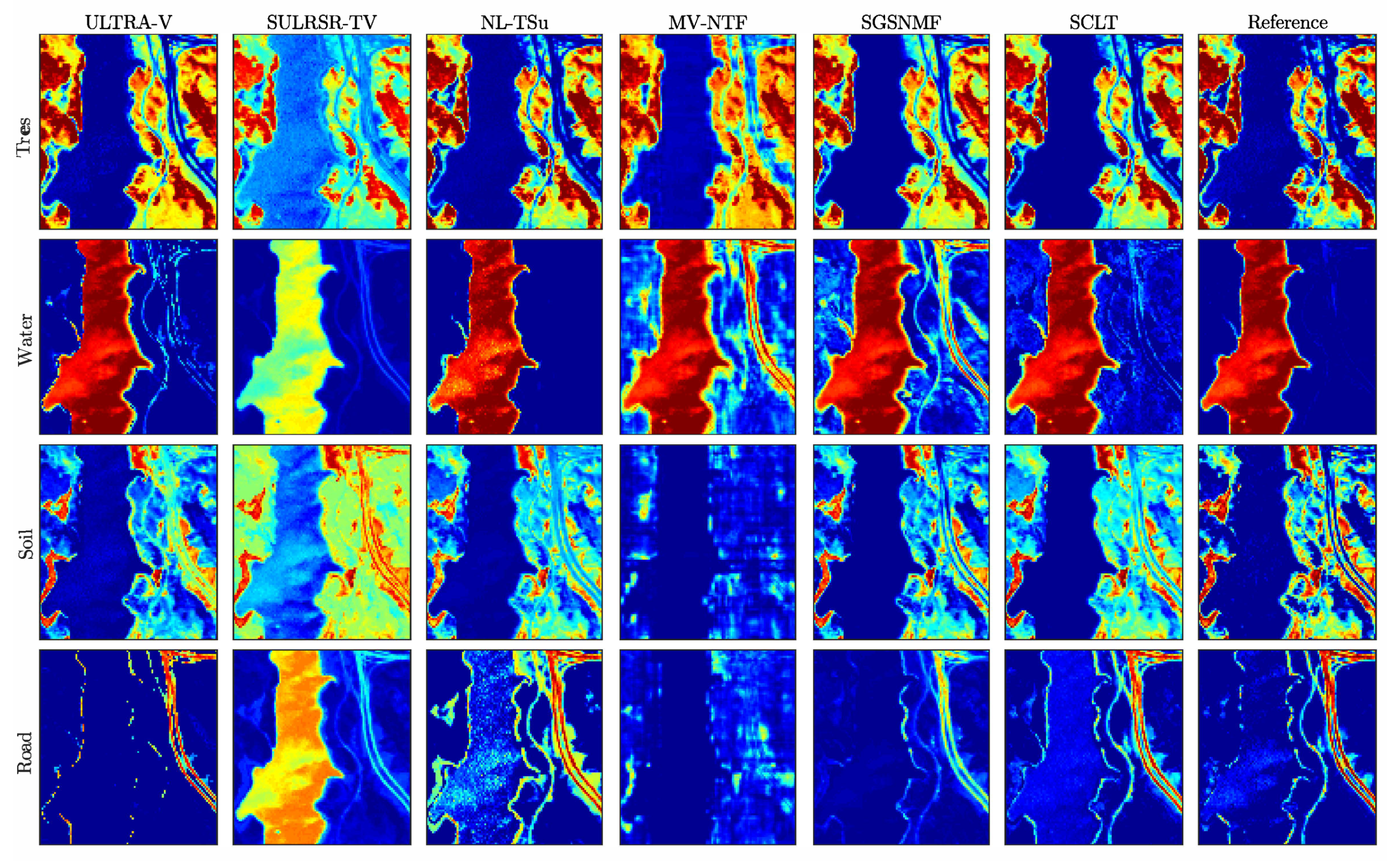
Mean	0.3863 ± 0.0357	0.3005 ± 0.0039	0.3024 ± 0.0396	0.3723 ± 0.0482	0.3002 ± 0.0010	0.2516 ± 0.0024

shows the SAD and its deviation results of the five comparison methods and the proposed SCLT algorithm on Jasper Ridge data. It can be concluded that the unmixing performance of the five algorithms on Jasper Ridge data is generally not high. The proposed SCLT algorithm just has significant advantages in extracting the endmember spectra of Soil. Although the superior performance of the SAD on the other three endmembers is not perfect, it is stable when extracting each spectrum, and the deviation is almost close to zero. Figure 2 and Figure 3 are visualization comparison of the unmixing results of the six algorithms. In Figure 2, the SCLT proposed in all abundance maps is the closest to the real reference abundance map, which shows the superiority of the proposed SCLT in abundance estimation. In Figure 3, the fourth spectral curve algorithm generally does not perform well, because it stands for the road spectrum, which requires a higher unmixing algorithm. It can be seen from this experiment that the proposed SCLT algorithm has a weak advantage over other algorithms on Jasper Ridge data.

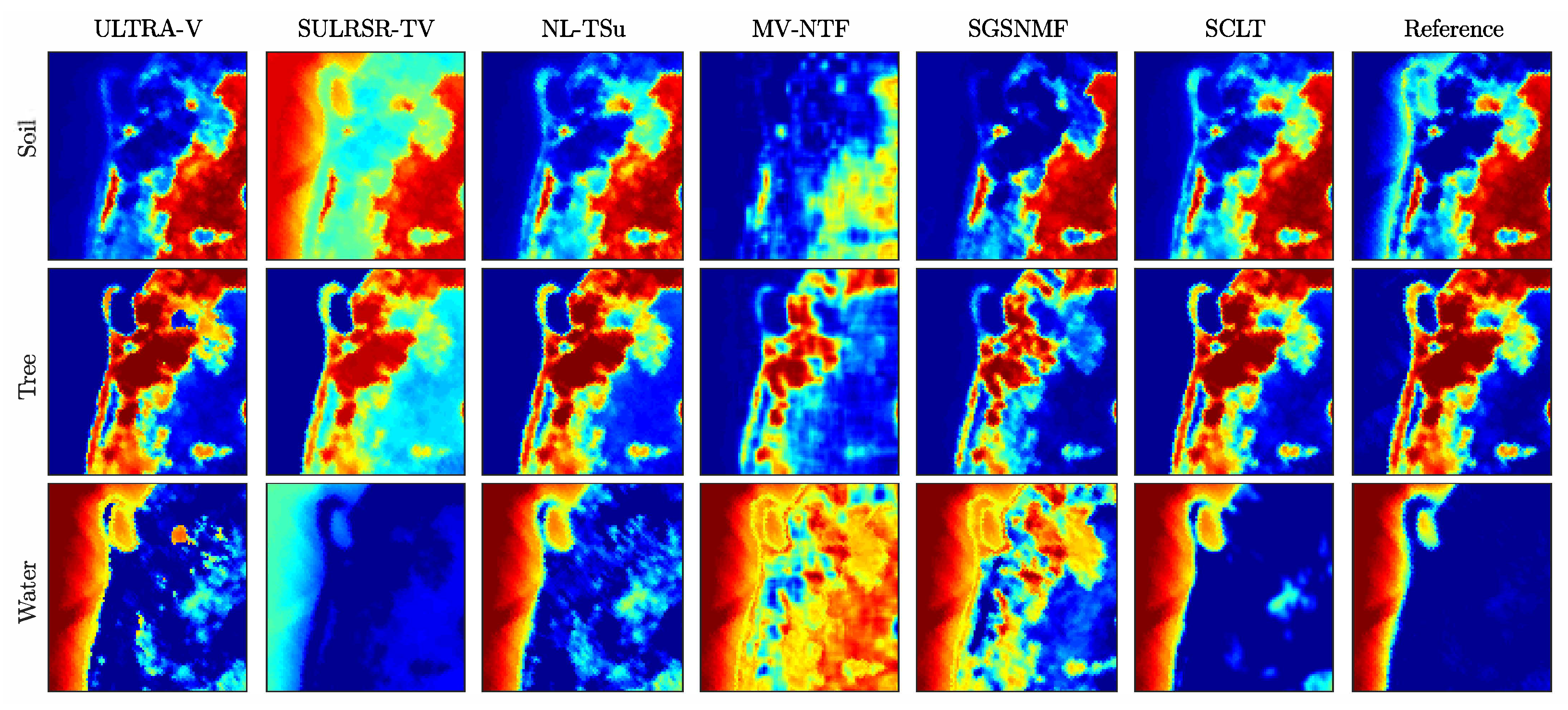
Samon Dataset. According to the existing research results [46], Samon data mainly contain three types of ground objects, including Soil, Tree and Water. These data have 156 bands, and the spectral band coverage is 0.401–0.889 μm. Since the original data is very large, a sub-image with a size of 95 × 95 is used in real experiments for saving space. Specifically, the pseudo-color image of Samon data is shown in Figure 1b. As shown in

Table 2. SAD results on the Samon data. Bold indicates the best unmixing result in each endmember.

	SULRSR-TV	SGSNMF	MV-NTF	NL-TSUn	ULTRA-V	SCLT
Tree	0.0247 ± 0.0121	0.0099 ± 0.0001	0.0433 ± 0.0129	0.0288 ± 0.0161	0.0340 ± 0.0272	0.0465 ± 0.0019
Water	0.0495 ± 0.0011	0.0511 ± 0.0017	0.0953 ± 0.0011	0.0496 ± 0.0001	0.0566 ± 0.0090	0.0648 ± 0.0006
Soil	0.1299 ± 0.0004	0.2189 ± 0.0024	0.2810 ± 0.0050	0.1289 ± 0.0003	0.2401 ± 0.0221	0.0937 ± 0.0031
Mean	0.0818 ± 0.0019	0.1299 ± 0.0011	0.1733 ± 0.0036	0.0825 ± 0.0026	0.1438 ± 0.0154	0.0711 ± 0.0002

, it is the quantitative comparison result of five comparison methods and the proposed SCLT on Samon data. It can be seen that SULRSR-TV, SGSNMF and SCLT all show better unmixing results on a single spectrum. However, these five comparison algorithms have poor performance on Soil. The SCLT not only has the best results on the average spectrum, but also has extremely high unmixing stability on each endmember with the smallest deviation. Specifically, the endmember spectral curves and estimated abundance maps extracted by the six unmixing methods in this experiment are presented in Figure 4 and Figure 5, respectively. They can also be confirmed from the visualizations, which show that the proposed SCLT method has the best unmixing performance.

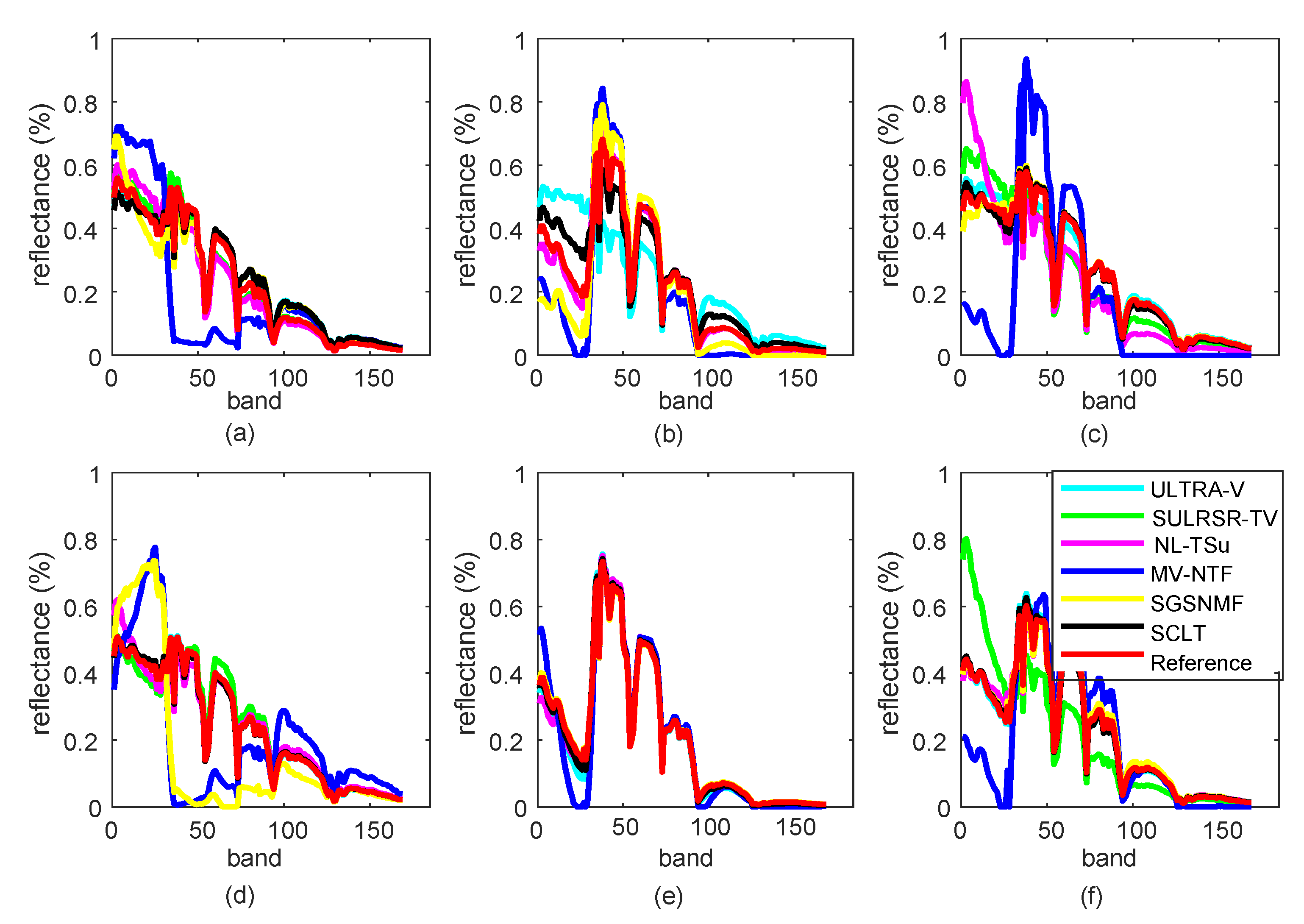
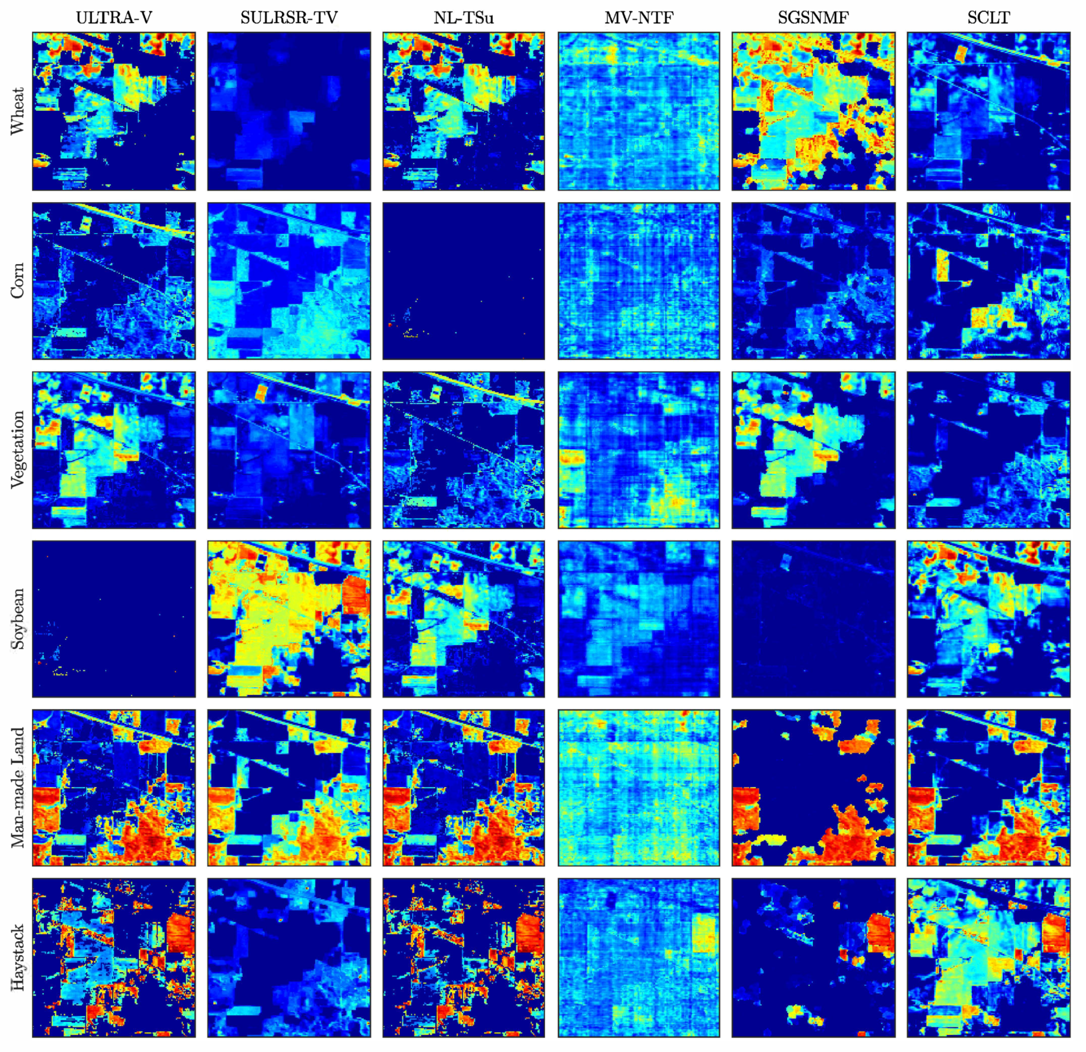
Indiana Pines Dataset. The Indiana Pines dataset is a database widely used for unmixing. It contains 224 bands, some of which are also affected by water vapor and have low signal-to-noise-ratio (SNR). Therefore, the selected Indiana Pines dataset has 169 bands and the spatial size is $145\times 145$. The pseudo-color image is shown in Figure 1c. Yuan et al. [41] points out that the Indiana Pines dataset mainly includes six kinds of materials, i.e., Wheat, Man-made land, Soybean, Corn, Vegetation and Haystack. The SAD results of six algorithms are shown in

Table 3. SAD results on the Indiana pines data. Bold indicates the best unmixing result in each endmember.

	SULRSR-TV	SGSNMF	MV-NTF	NL-TSUn	ULTRA-V	SCLT
Man-made land	0.0942 ± 0.0226	0.1266 ± 0.0618	0.5500 ± 0.1006	0.1090 ± 0.0128	0.0973 ± 0.0107	0.0938 ± 0.0007
Wheat	0.2861 ± 0.2175	0.3439 ± 0.2205	0.3730 ± 0.0374	0.3320 ± 0.1958	0.4456 ± 0.0028	0.4203 ± 0.0793
Corn	0.2669 ± 0.0746	0.0608 ± 0.0235	0.7127 ± 0.0294	0.2022 ± 0.1006	0.0807 ± 0.0310	0.0774 ± 0.0100
Soybean	0.0867 ± 0.0084	0.0608 ± 0.0235	0.4952 ± 0.1611	0.1138 ± 0.0713	0.0090 ± 0.0011	0.0089 ± 0.0036
Vegetation	0.0624 ± 0.0092	0.0270 ± 0.0151	0.2666 ± 0.0539	0.0651 ± 0.0085	0.0730 ± 0.0063	0.0689 ± 0.0128
Haystack	0.1375 ± 0.1453	0.0611 ± 0.0363	0.4638 ± 0.0661	0.0725 ± 0.0812	0.0381 ± 0.0321	0.0375 ± 0.0018
Mean	0.2079 ± 0.0352	0.3225 ± 0.0340	0.5041 ± 0.0184	0.1993 ± 0.0353	0.1921 ± 0.0011	0.1618 ± 0.0312

. It can be concluded that the SCLT algorithm has extremely superior performance in terms of stability, which is consistent with the unmixing results of Jasper data and Samon data. Although the proposed SCLT algorithm does not have the lowest error on each endmember spectrum, its average value is the smallest. Figure 6 introduces the endmember spectrum comparison curves extracted by six algorithms. Since the Indiana Dataset does not have the ground truth of abundances, here we only show the comparison of the abundance maps in Figure 7, and the results are similar to [8], which is sufficient to prove that the proposed SCLT algorithm has full superiority.

5.3. Parameter Analysis

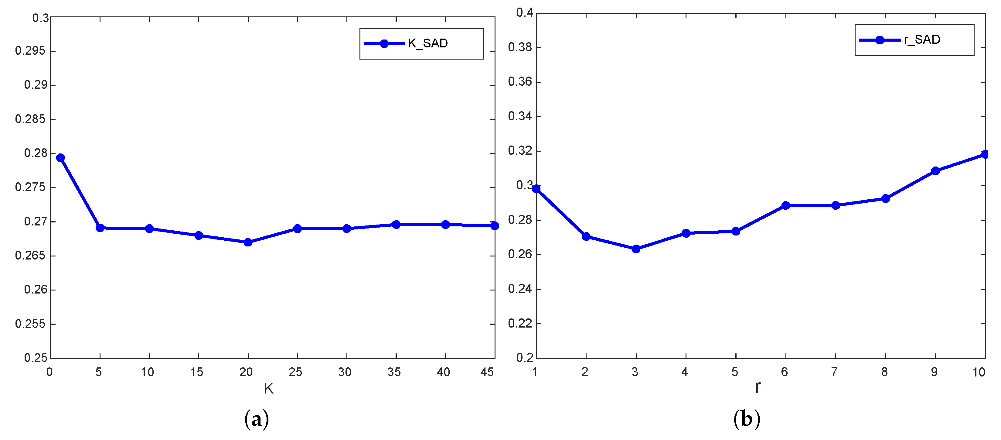
The parameters involved in the SCLT algorithm are discussed in this subsection, which mainly include the weight parameters of the low-rank regularization ${\lambda }_{LR}$ and the sparse constraint ${\lambda }_S$, the size r of the patch and the number K of the similarity group. Due to space limitations, here the Jasper Ridge dataset is taken as an example to illustrate how this paper evaluates the parameters. According to [8], the control variable method is used to determine the parameters. Firstly, ${\lambda }_{LR}$, ${\lambda }_S$ and r are set 0.01, 0.01 and 5, respectively. K is set to $\{1,5,10,15,20,25,30,35,40,45\}$. It can be seen from Figure 8a that, when K is 20, the unmixing achieves the best performance. Subsequently, K is fixed to 20. r is set to $\{1,2,3,4,5,6,7,8,9,10\}$. Figure 8b shows the SAD results under these parameter settings. It can be concluded that when $r=3$, the SCLT algorithm achieves the best performance on Jasper Ridge dataset.

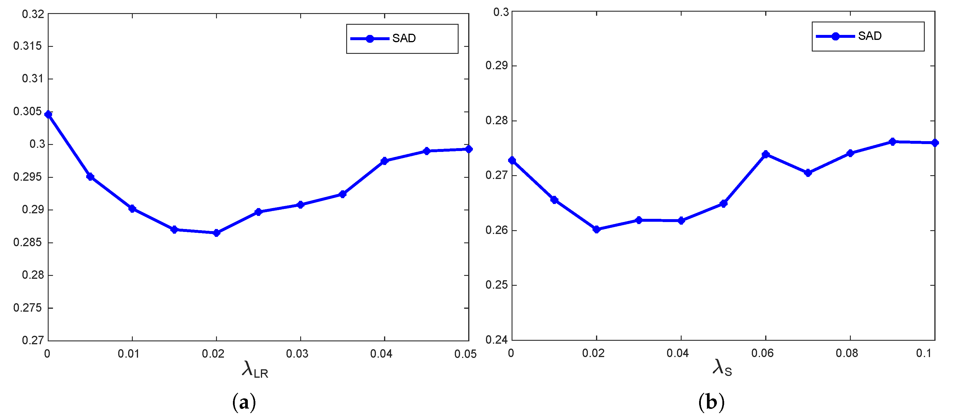
Finally, two regularization parameters are discussed, where ${\lambda }_{LR}$ represents the proposed low-rank regularization, and ${\lambda }_S$ represents the weight of the sparsity constraint. ${\lambda }_{LR}$ is set $\{0,0.5\times {10}^{-3},1\times {10}^{-2},1.5\times {10}^{-2},2\times {10}^{-2},2.5\times {10}^{-2},3\times {10}^{-2},3.\times {10}^{-2},4\times {10}^{-2},4.5\times {10}^{-2},5\times {10}^{-2}\}$ in turn when ${\lambda }_S$ is 0.01. Then ${\lambda }_{LR}$ is fixed 0.02, ${\lambda }_S$ is set $\{0,1\times {10}^{-2},2\times {10}^{-2},3\times {10}^{-2},4\times {10}^{-2},5\times {10}^{-2},6\times {10}^{-2},7\times {10}^{-2},8\times {10}^{-2},9\times {10}^{-2},1\times {10}^{-1}\}$ in turn. In the discussion of these two parameters, a value of zero is set, the purpose of which is to prove the effectiveness of each term of the proposed algorithm. When ${\lambda }_{LR}$ is zero, SCLT only adds the sparse constraint. When ${\lambda }_S$ is zero, the algorithm only adds the low-rank constraint. It can be understood from the unmixing results in Figure 9 that when ${\lambda }_{LR}$ = 0.02 and ${\lambda }_S$ = 0.020, the SCLT algorithm reaches the optimal solution, which also proves the effectiveness of each constraint of the algorithm. Consistent with the method discussed above, the parameter settings of the remaining experiments are presented in

Table 4. Parameter settings.

Data	K	r	${\mathit{\lambda }}_{\mathbf{LR}}$	${\mathit{\lambda }}_{\mathit{S}}$
Jasper	20	3	0.020	0.02
Samon	20	3	0.015	0.01
Indiana	50	5	0.010	0.01

.

6. Conclusions

In this paper, we propose a novel non-negative tensor factorization framework by combining a low tensor rank constraint and a $L_{2,1}$ sparsity constraint for hyperspectral unmixing. A regularization that can describe the low-rank properties of HSI is designed to learn the low-rank structure of the similarity groups along the spatial, spectral and non-local similarity modes in the image. In addition, the $L_{2,1}$ norm is applied to explore the sparseness of abundances. The proposed unmixing framework SCLT can not only learn the low-rank structure of data in the different modes, but also keep the sparseness of the abundance. The SCLT is optimized by the ADMM method. The experimental results conducted on three real data introduce the superiority and effectiveness of the proposed algorithm.

References

1. Lu, X.; Sun, H.; Zheng, X. A Feature Aggregation Convolutional Neural Network for Remote Sensing Scene Classification. IEEE Trans. Geosci. Remote Sens. 2019, 57, 7894–7906. [Google Scholar] [CrossRef]
2. Hong, D.; Gao, L.; Yao, J.; Zhang, B.; Plaza, A.; Chanussot, J. Graph Convolutional Networks for Hyperspectral Image Classification. IEEE Trans. Geosci. Remote Sens. 2020, 1–13. [Google Scholar] [CrossRef]
3. Fan, X.; Zhang, Y.; Li, F.; Chen, Y.; Shao, T.; Zhou, S. A robust spectral target recognition method for hyperspectral data based on combined spectral signatures. In Proceedings of the 2011 IEEE International Geoscience and Remote Sensing Symposium, Vancouver, BC, Canada, 24–29 July 2011; pp. 4328–4331. [Google Scholar]
4. Zhang, W.; Lu, X.; Li, X. Similarity Constrained Convex Nonnegative Matrix Factorization for Hyperspectral Anomaly Detection. IEEE Trans. Geosci. Remote Sens. 2019, 57, 4810–4822. [Google Scholar] [CrossRef]
5. Sun, H.; Li, S.; Zheng, X.; Lu, X. Remote Sensing Scene Classification by Gated Bidirectional Network. IEEE Trans. Geosci. Remote Sens. 2020, 58, 82–96. [Google Scholar] [CrossRef]
6. Boardman, J.W. Mapping target signatures via partial unmixing of aviris data. In Proceedings of the JPL Airborne Geoscience Workshop, Pasadena, CA, USA, 23–26 January 1995. [Google Scholar]
7. Zhang, B.; Sun, X.; Gao, L.; Yang, L. Endmember Extraction of Hyperspectral Remote Sensing Images Based on the Ant Colony Optimization (ACO) Algorithm. IEEE Trans. Geosci. Remote Sens. 2011, 49, 2635–2646. [Google Scholar] [CrossRef]
8. Lu, X.; Dong, L.; Yuan, Y. Subspace Clustering Constrained Sparse NMF for Hyperspectral Unmixing. IEEE Trans. Geosci. Remote Sens. 2020, 58, 3007–3019. [Google Scholar] [CrossRef]
9. Kizel, F.; Benediktsson, J.A. Spatially Enhanced Spectral Unmixing Through Data Fusion of Spectral and Visible Images from Different Sensors. Remote Sens. 2020, 12, 1255. [Google Scholar] [CrossRef] [Green Version]
10. Miao, L.; Qi, H. Endmember Extraction From Highly Mixed Data Using Minimum Volume Constrained Nonnegative Matrix Factorization. IEEE Trans. Geosci. Remote Sens. 2007, 45, 765–777. [Google Scholar] [CrossRef]
11. Zhang, Z.; Liao, S.; Zhang, H.; Wang, S.; Wang, Y. Bilateral Filter Regularized L2 Sparse Nonnegative Matrix Factorization for Hyperspectral Unmixing. Remote Sens. 2018, 10, 816. [Google Scholar] [CrossRef] [Green Version]
12. Guo, Z.; Wittman, T.; Osher, S. L1 unmixing and its application to hyperspectral image enhancement. International Society for Optics and Photonics. In Proceedings of the SPIE Defense, Security, and Sensing, Orlando, FL, USA, 13 March 2009. [Google Scholar]
13. Qian, Y.; Jia, S.; Zhou, J.; Robles-Kelly, A. Hyperspectral unmixing via L_{1/2} sparsity-constrained nonnegative matrix factorization. IEEE Trans. Geosci. Remote Sens. 2011, 49, 4282–4297. [Google Scholar] [CrossRef] [Green Version]
14. Xu, Z.; Chang, X.; Xu, F.; Zhang, H. L1/2 regularization: A thresholding representation theory and a fast solver. IEEE Trans. Neural Netw. Learn. Syst. 2012, 23, 1013. [Google Scholar] [PubMed]
15. Yao, J.; Meng, D.; Zhao, Q.; Cao, W.; Xu, Z. Nonconvex-Sparsity and Nonlocal-Smoothness-Based Blind Hyperspectral Unmixing. IEEE Trans. Image Process. 2019, 28, 2991–3006. [Google Scholar] [CrossRef] [PubMed]
16. Salehani, Y.E.; Gazor, S. Smooth and Sparse Regularization for NMF Hyperspectral Unmixing. IEEE J. Sel. Top. Appl. Earth Obs. Remote Sens. 2017, 10, 3677–3692. [Google Scholar] [CrossRef]
17. Yang, L.; Peng, J.; Su, H.; Xu, L.; Wang, Y.; Yu, B. Combined Nonlocal Spatial Information and Spatial Group Sparsity in NMF for Hyperspectral Unmixing. IEEE Geosci. Remote Sens. Lett. 2020, 17, 1767–1771. [Google Scholar] [CrossRef]
18. Wang, H.; Yang, W.; Guan, N. Cauchy sparse NMF with manifold regularization: A robust method for hyperspectral unmixing. Knowl. Based Syst. 2019, 184, 104898.1–104898.16. [Google Scholar] [CrossRef]
19. Wang, M.; Zhang, B.; Pan, X.; Yang, S. Group Low-Rank Nonnegative Matrix Factorization with Semantic Regularizer for Hyperspectral Unmixing. IEEE J. Sel. Top. Appl. Earth Obs. Remote Sens. 2018, 11, 1022–1029. [Google Scholar] [CrossRef]
20. Zheng, Y.; Wu, F.; Shim, H.J.; Sun, L. Sparse Unmixing for Hyperspectral Image with Nonlocal Low-Rank Prior. Remote Sens. 2019, 11, 2897. [Google Scholar] [CrossRef] [Green Version]
21. Hong, D.; Yokoya, N.; Chanussot, J.; Zhu, X.X. An Augmented Linear Mixing Model to Address Spectral Variability for Hyperspectral Unmixing. IEEE Trans. Image Process. 2019, 28, 1923–1938. [Google Scholar] [CrossRef] [PubMed] [Green Version]
22. Qian, Y.; Xiong, F.; Zeng, S.; Zhou, J.; Tang, Y.Y. Matrix-Vector Nonnegative Tensor Factorization for Blind Unmixing of Hyperspectral Imagery. IEEE Trans. Geosci. Remote Sens. 2017, 55, 1776–1792. [Google Scholar] [CrossRef] [Green Version]
23. Bilius, L.B.; Pentiuc, S.G. Improving the Analysis of Hyperspectral Images Using Tensor Decomposition. In Proceedings of the 2020 International Conference on Development and Application Systems (DAS), Suceava, Romania, 21–23 May 2020. [Google Scholar]
24. Chatzichristos, C.; Kofidis, E.; Morante, M.; Theodoridis, S. Blind fMRI Source Unmixing via Higher-Order Tensor Decompositions. J. Neurosci. Methods 2019, 315, 17–47. [Google Scholar] [CrossRef]
25. Xiong, F.; Chen, J.; Zhou, J.; Qian, Y. Superpixel-Based Nonnegative Tensor Factorization for Hyperspectral Unmixing. In Proceedings of the IGARSS 2018—2018 IEEE International Geoscience and Remote Sensing Symposium, Valencia, Spain, 22–27 July 2018; pp. 6392–6395. [Google Scholar]
26. Xiong, F.; Qian, Y.; Zhou, J.; Tang, Y.Y. Hyperspectral Unmixing via Total Variation Regularized Nonnegative Tensor Factorization. IEEE Trans. Geosci. Remote Sens. 2019, 57, 2341–2357. [Google Scholar] [CrossRef]
27. Yuan, B. NMF hyperspectral unmixing algorithm combined with spatial and spectral correlation analysis. J. Remote Sens. 2018, 22, 265–276. [Google Scholar]
28. Yuan, Y.; Feng, Y.; Lu, X. Projection-Based NMF for Hyperspectral Unmixing. IEEE J. Sel. Top. Appl. Earth Obs. Remote Sens. 2015, 8, 2632–2643. [Google Scholar] [CrossRef]
29. Xu, Z.; Zhang, H.; Wang, Y.; Chang, X.; Liang, Y. L 1/2 regularization. Sci. China Inf. Sci. 2010, 53, 1159–1169. [Google Scholar] [CrossRef] [Green Version]
30. Pauca, V.P.; Piper, J.; Plemmons, R.J. Nonnegative matrix factorization for spectral data analysis. Linear Algebra Its Appl. 2006, 416, 29–47. [Google Scholar] [CrossRef] [Green Version]
31. Li, M.; Zhu, F.; Guo, A.J.X. A Robust Multilinear Mixing Model with l 2,1 norm for Unmixing Hyperspectral Images. In Proceedings of the 2020 IEEE International Conference on Visual Communications and Image Processing (VCIP), Macau, China, 1–4 December 2020. [Google Scholar]
32. Ma, Y.; Li, C.; Mei, X.; Liu, C.; Ma, J. Robust Sparse Hyperspectral Unmixing with 2,1 Norm. IEEE Trans. Geosci. Remote Sens. 2017, 55, 1227–1239. [Google Scholar] [CrossRef]
33. Huang, J.; Huang, T.Z.; Zhao, X.L.; Deng, L.J. Nonlocal Tensor-Based Sparse Hyperspectral Unmixing. IEEE Trans. Geosci. Remote Sens. 2020, 1–15. [Google Scholar] [CrossRef]
34. Feng, B.; Wang, J. Constrained Nonnegative Tensor Factorization for Spectral Unmixing of Hyperspectral Images: A Case Study of Urban Impervious Surface Extraction. IEEE Geosci. Remote Sens. Lett. 2019, 16, 583–587. [Google Scholar] [CrossRef]
35. Imbiriba, T.; Borsoi, R.A.; Bermudez, J.C.M. Low-Rank Tensor Modeling for Hyperspectral Unmixing Accounting for Spectral Variability. IEEE Trans. Geosci. Remote Sens. 2020, 58, 1833–1842. [Google Scholar] [CrossRef] [Green Version]
36. Sun, L.; Wu, F.; Zhan, T.; Liu, W.; Wang, J.; Jeon, B. Weighted Nonlocal Low-Rank Tensor Decomposition Method for Sparse Unmixing of Hyperspectral Images. IEEE J. Sel. Top. Appl. Earth Obs. Remote Sens. 2020, 13, 1174–1188. [Google Scholar] [CrossRef]
37. Zhang, S.; Zhang, G.; Deng, C.; Li, J.; Wang, S.; Wang, J.; Plaza, A. Spectral-Spatial Weighted Sparse Nonnegative Tensor Factorization for Hyperspectral Unmixing. In Proceedings of the IGARSS 2020—2020 IEEE International Geoscience and Remote Sensing Symposium, Online. 26 September–2 October 2020; pp. 2177–2180. [Google Scholar]
38. Arthur, D.; Vassilvitskii, S. K-Means++: The Advantages of Careful Seeding. In Proceedings of the Eighteenth Acm-siam Symposium on Discrete Algorithms, Philadelphia, PA, USA, 7–9 January 2007. [Google Scholar]
39. Dian, R.; Li, S.; Fang, L. Learning a Low Tensor-Train Rank Representation for Hyperspectral Image Super-Resolution. IEEE Trans. Neural Netw. Learn. Syst. 2019, 30, 2672–2683. [Google Scholar] [CrossRef]
40. Akhtar, N.; Mian, A. RCMF: Robust Constrained Matrix Factorization for Hyperspectral Unmixing. IEEE Trans. Geosci. Remote Sens. 2017, 55, 3354–3366. [Google Scholar] [CrossRef]
41. Yuan, Y.; Fu, M.; Lu, X. Substance Dependence Constrained Sparse NMF for Hyperspectral Unmixing. IEEE Trans. Geosci. Remote Sens. 2015, 53, 2975–2986. [Google Scholar] [CrossRef]
42. Li, H.; Feng, R.; Wang, L.; Zhong, Y.; Zhang, L. Superpixel-Based Reweighted Low-Rank and Total Variation Sparse Unmixing for Hyperspectral Remote Sensing Imagery. IEEE Trans. Geosci. Remote Sens. 2021, 59, 629–647. [Google Scholar] [CrossRef]
43. Wang, X.; Zhong, Y.; Zhang, L.; Xu, Y. Spatial group sparsity regularized nonnegative matrix factorization for hyperspectral unmixing. IEEE Trans. Geosci. Remote Sens. 2017, 55, 6287–6304. [Google Scholar] [CrossRef]
44. Nascimento, J.M.P.; Dias, J.M.B. Vertex component analysis: A fast algorithm to unmix hyperspectral data. IEEE Trans. Geosci. Remote Sens. 2005, 43, 898–910. [Google Scholar] [CrossRef] [Green Version]
45. Wang, W.; Liu, H. Deep Nonnegative Dictionary Factorization for Hyperspectral Unmixing. Remote Sens. 2020, 12, 2882. [Google Scholar] [CrossRef]
46. Zhu, F.; Wang, Y.; Fan, B.; Xiang, S.; Meng, G.; Pan, C. Spectral Unmixing via Data-Guided Sparsity. IEEE Trans. Image Process. 2014, 23, 5412–5427. [Google Scholar] [CrossRef] [Green Version]
Figure 1. Three real hyperspectral datasets. (a) Jasper Ridge. (b) Samon. (c) Indiana.
Remotesensing 13 01473 g001
Figure 2. The abundance maps of six methods and the ground truth on Jasper Ridge Data.
Remotesensing 13 01473 g002
Figure 3. The endmember spectra of Jasper Ridge Data extracted by the five comparison methods and the proposed method. (a) Tree. (b) Soil. (c) Water. (d) Road.
Remotesensing 13 01473 g003
Figure 4. The endmember spectra of Samon Data extracted by the five comparison methods and the proposed method. (a) Soil. (b) Tree. (c) Water.
Remotesensing 13 01473 g004
Figure 5. The abundance maps of six methods and the Ground Truth on Samon Data.
Remotesensing 13 01473 g005
Figure 6. The endmember spectra of Indiana Pines Data extracted by the five comparison methods and the proposed method. (a) Man-made land. (b) Wheat. (c) Corn. (d) Soybean. (e) Vegetation. (f) Haystack.
Remotesensing 13 01473 g006
Figure 7. The abundance maps of six methods on Indiana Pines Data.
Remotesensing 13 01473 g007
Figure 8. Algorithm parameter analysis on the Jasper Ridge dataset. (a) Parameter K; (b) Parameter r.
Remotesensing 13 01473 g008
Figure 9. Algorithm parameter analysis on the Jasper Ridge dataset. (a) Parameter λ L R ; (b) Parameter λ S .
Remotesensing 13 01473 g009