
Automated Global Shallow Water Bathymetry Mapping Using Google Earth Engine

 , ,
, ,  ,
,  ,
, 
Abstract
1. Introduction
2. Materials and Methods
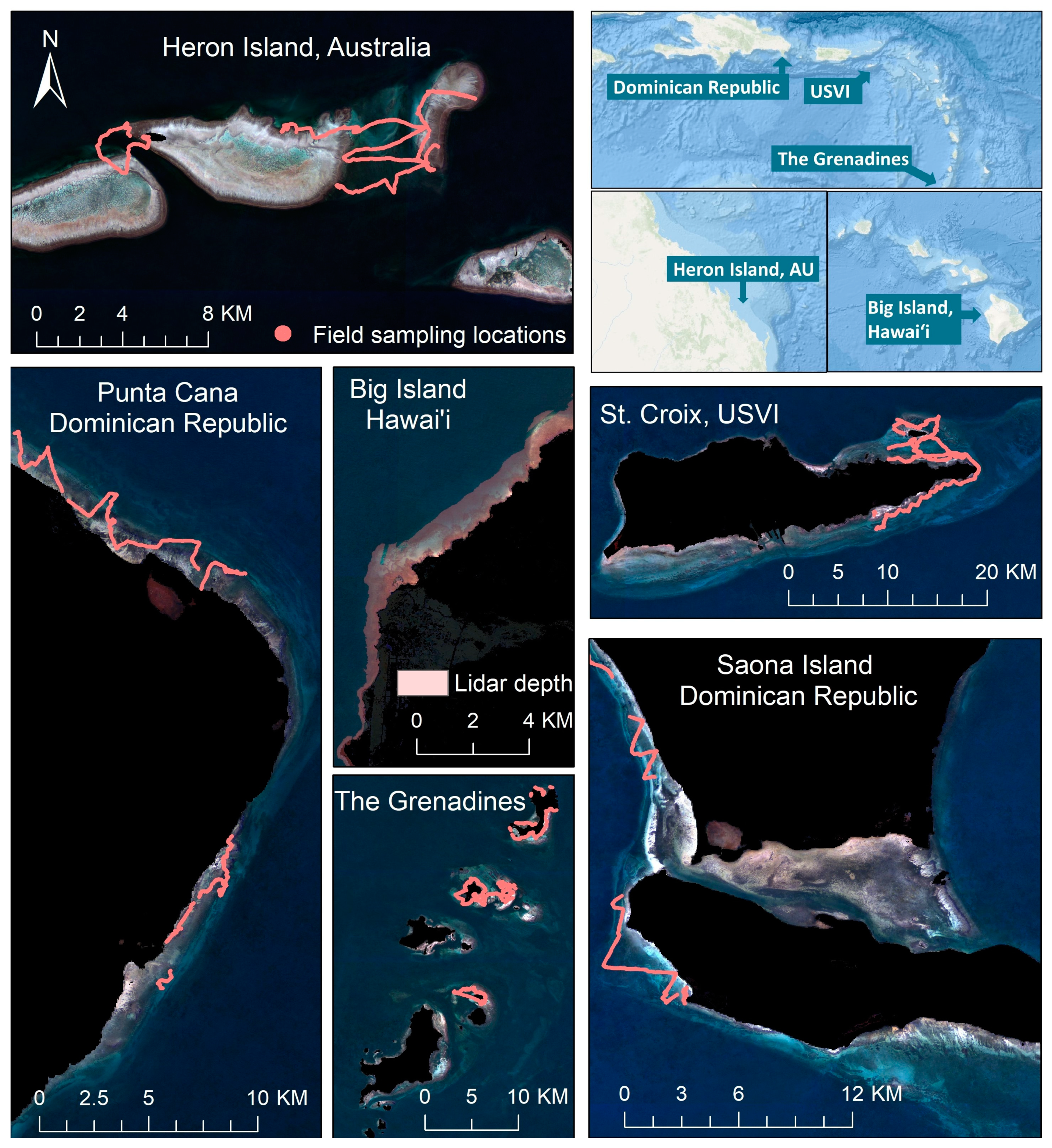
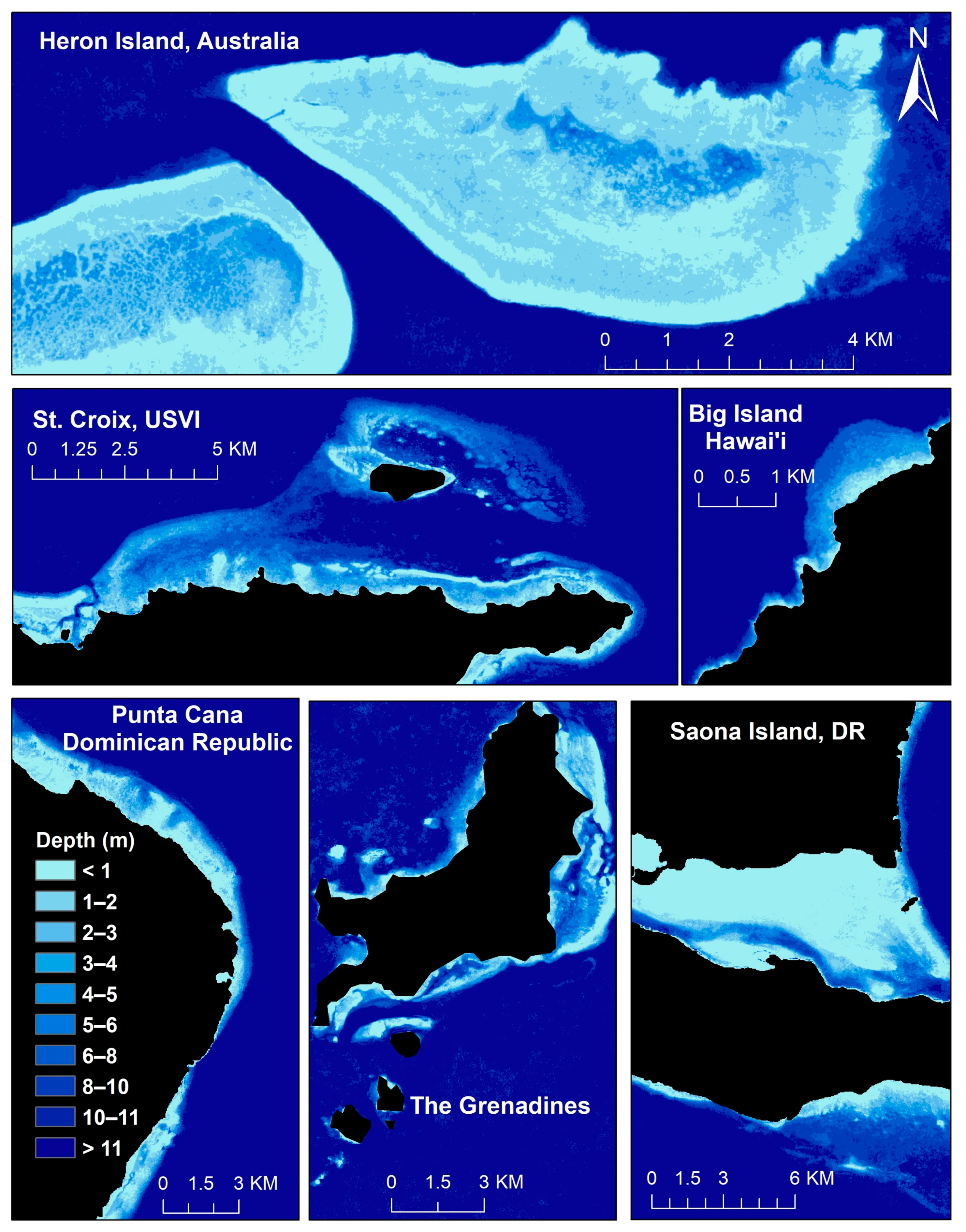
2.1. Study Sites and Data
2.2. Clean Water Mosaic Generation Using Google Earth Engine
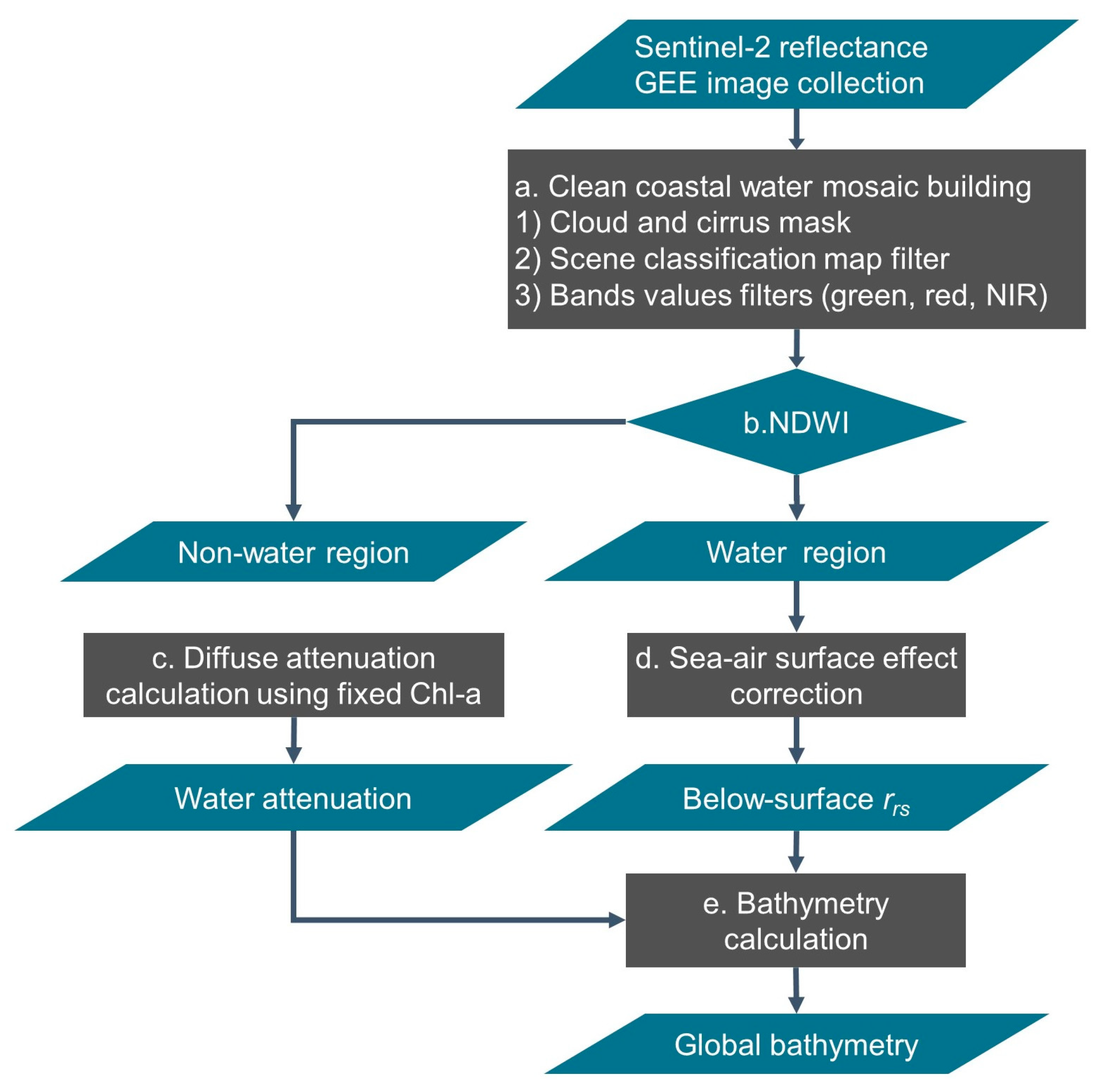
2.3. An Automatic Bathymetry Estimation Algorithm
3. Results
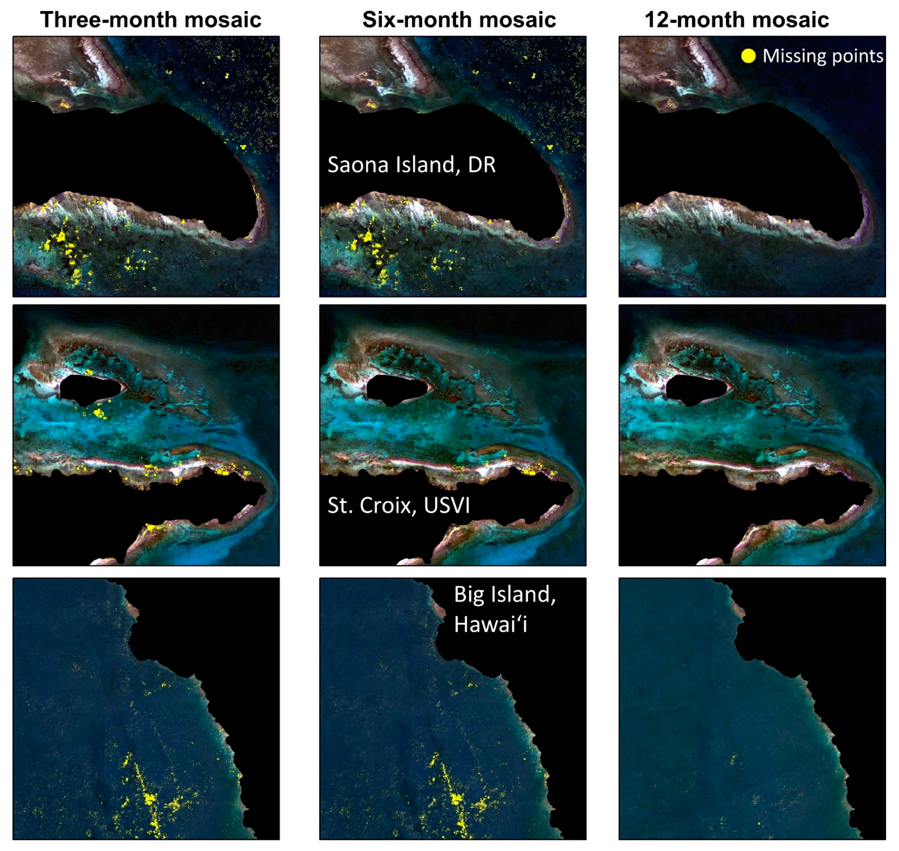
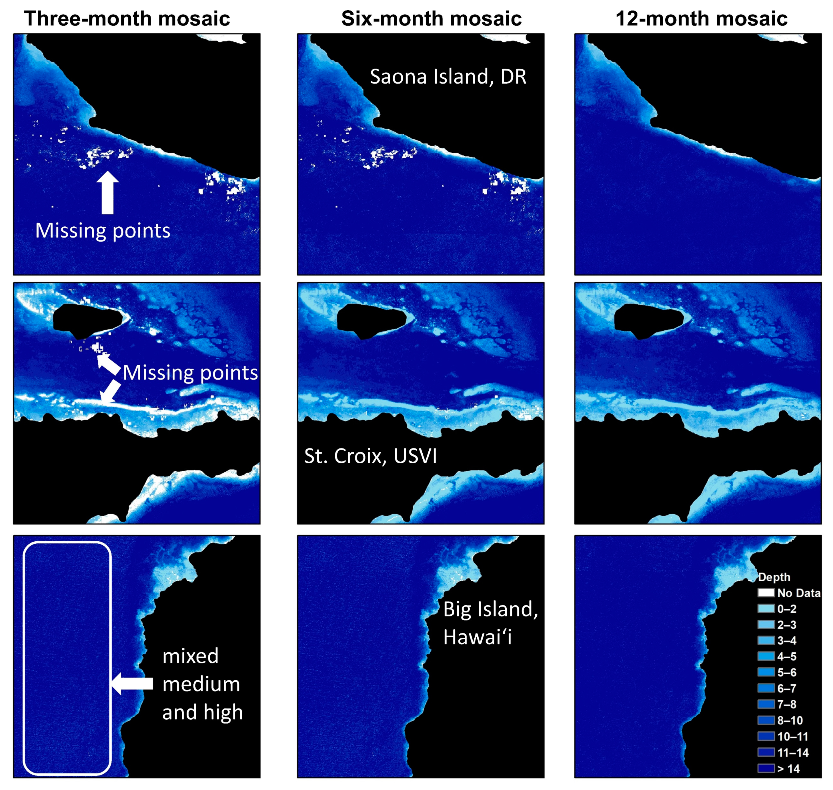
3.1. Clean Shallow Water Mosaic Created from Google Earth Engine
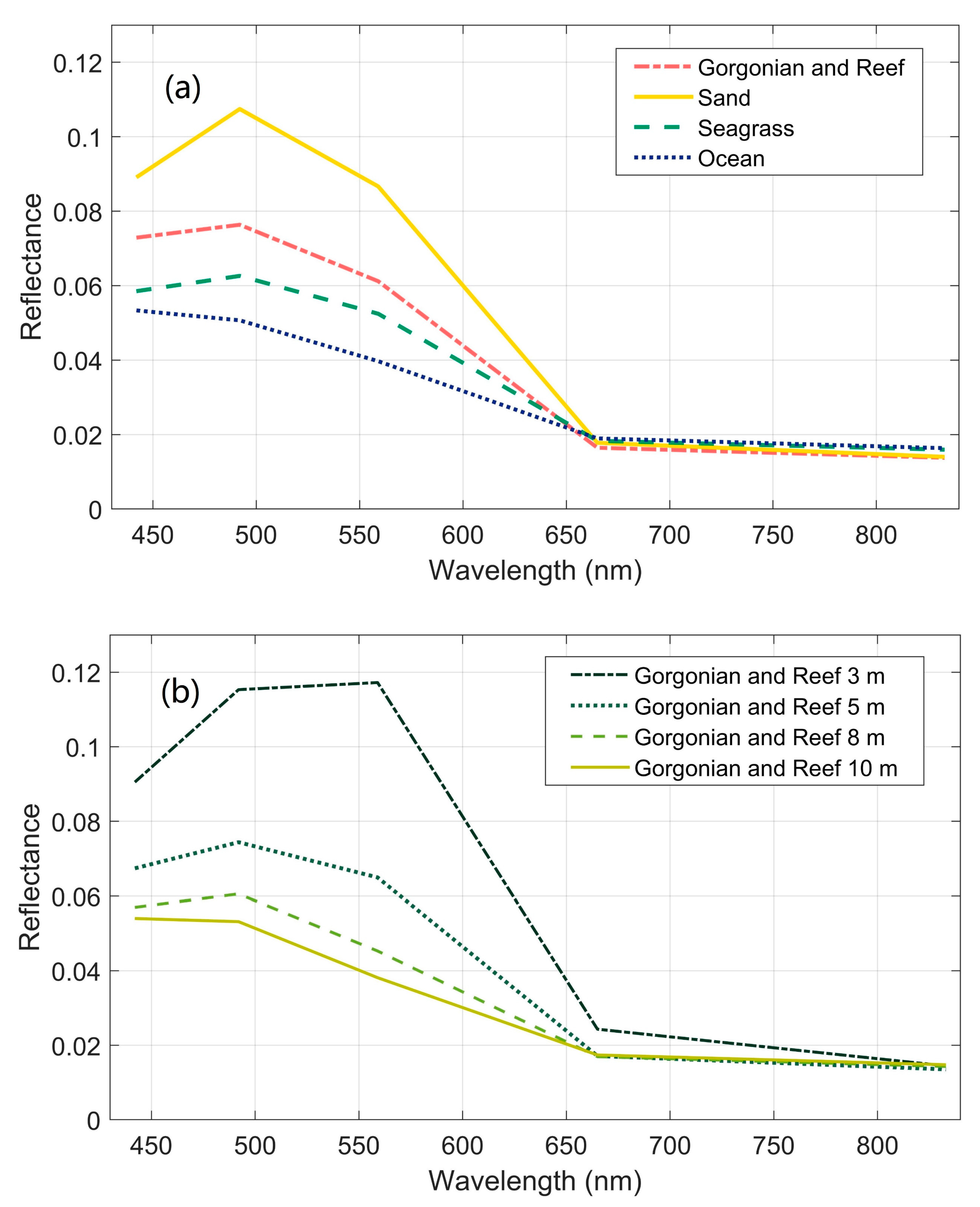
3.2. Bathymetry Spatial Variation Analysis
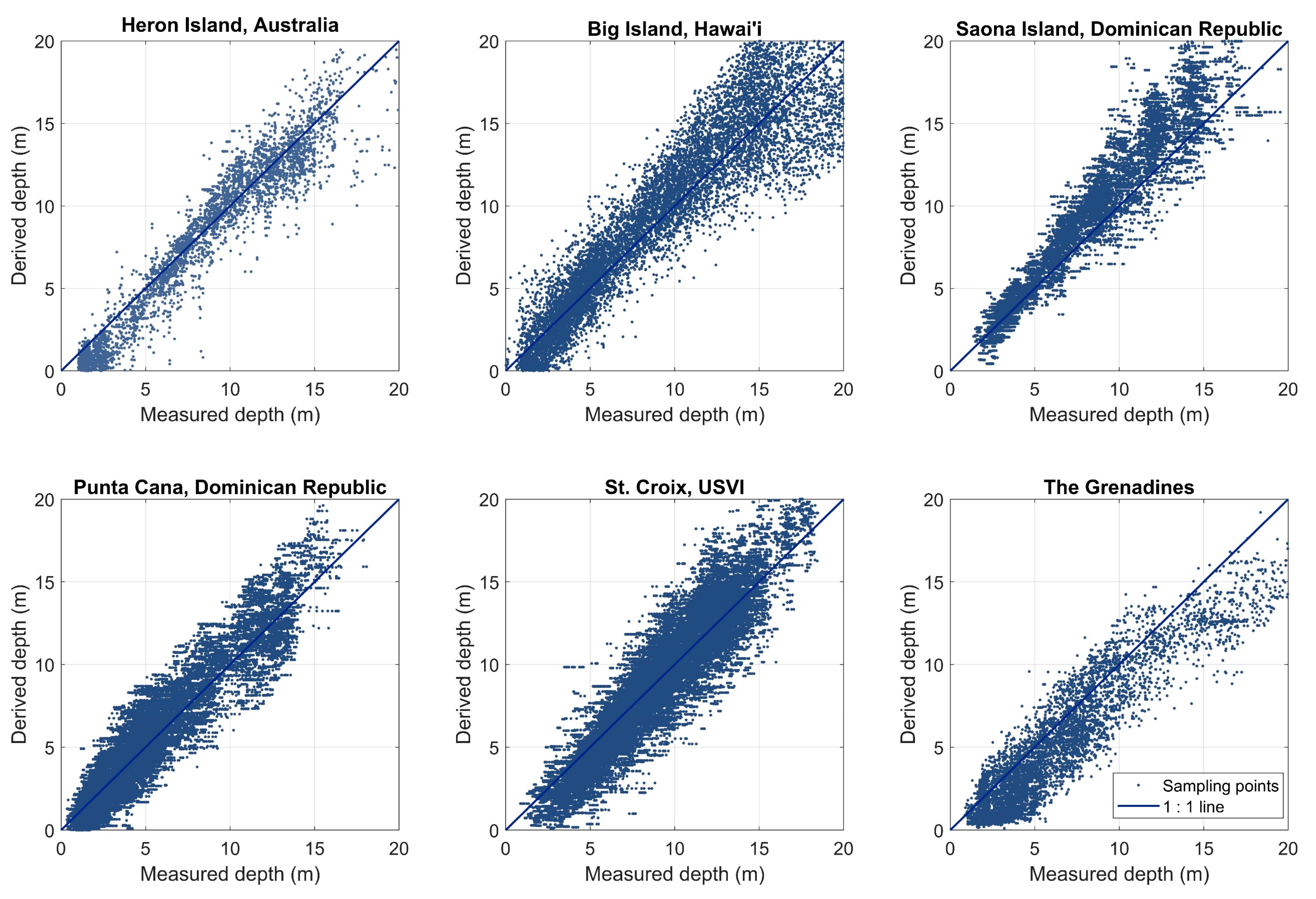
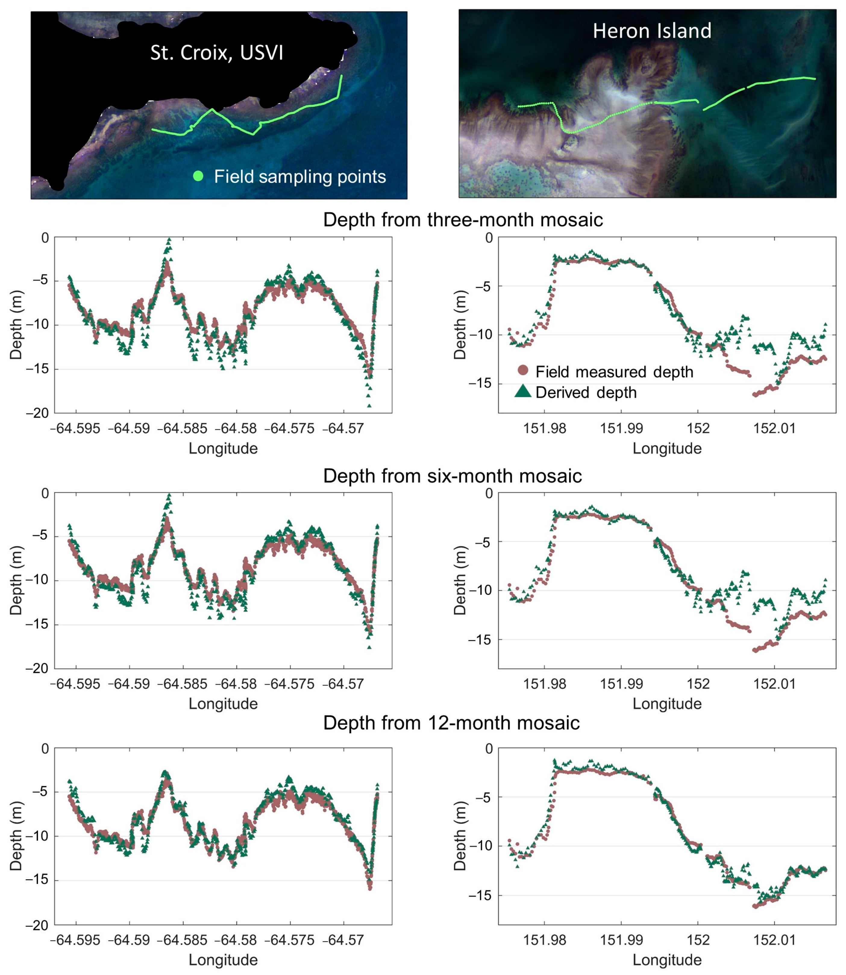
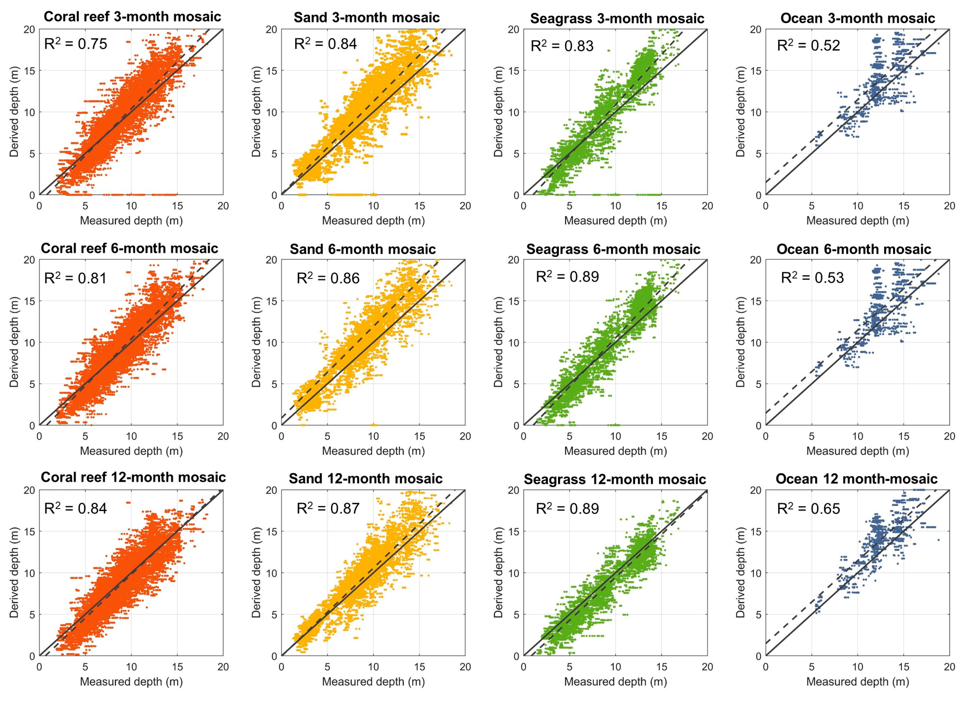
3.3. Evaluation of Bathymetry Estimation
3.4. Bathymetry Estimation Performance Impacted by Mosaic, Depth and Bottom Conditions
4. Discussion
5. Conclusions
Author Contributions
Funding
Data Availability Statement
Conflicts of Interest
References
- Kutser, T.; Miller, I.; Jupp, D.L. Mapping Coral Reef Benthic Substrates Using Hyperspectral Space-Borne Images and Spectral Libraries. Estuar. Coast. Shelf Sci. 2006, 70, 449–460. [Google Scholar] [CrossRef]
- Lyons, M.B.; Roelfsema, C.M.; Kennedy, E.V.; Kovacs, E.M.; Borrego-Acevedo, R.; Markey, K.; Roe, M.; Yuwono, D.M.; Harris, D.L.; Phinn, S.R.; et al. Mapping the World’s Coral Reefs Using a Global Multiscale Earth Observation Framework. Remote Sens. Ecol. Conserv. 2020. [Google Scholar] [CrossRef]
- Moberg, F.; Folke, C. Ecological Goods and Services of Coral Reef Ecosystems. Ecol. Econ. 1999, 29, 215–233. [Google Scholar] [CrossRef]
- Purkis, S.J. Remote Sensing Tropical Coral Reefs: The View from Above. Annu. Rev. Mar. Sci. 2018, 10, 149–168. [Google Scholar] [CrossRef] [PubMed]
- Roelfsema, C.; Kovacs, E.; Ortiz, J.C.; Wolff, N.H.; Callaghan, D.; Wettle, M.; Ronan, M.; Hamylton, S.M.; Mumby, P.J.; Phinn, S. Coral Reef Habitat Mapping: A Combination of Object-Based Image Analysis and Ecological Modelling. Remote Sens. Environ. 2018, 208, 27–41. [Google Scholar] [CrossRef]
- Asner, G.P.; Martin, R.E.; Mascaro, J. Coral Reef Atoll Assessment in the South China Sea Using Planet Dove Satellites. Remote Sens. Ecol. Conserv. 2017, 3, 57–65. [Google Scholar] [CrossRef]
- Barbier, E.B.; Koch, E.W.; Silliman, B.R.; Hacker, S.D.; Wolanski, E.; Primavera, J.; Granek, E.F.; Polasky, S.; Aswani, S.; Cramer, L.A. Coastal Ecosystem-Based Management with Nonlinear Ecological Functions and Values. Science 2008, 319, 321–323. [Google Scholar] [CrossRef] [PubMed]
- Bruckner, A.W. Life-Saving Products from Coral Reefs. Issues Sci. Technol. 2002, 18, 39–44. [Google Scholar]
- Carr, M.H.; Anderson, T.W.; Hixon, M.A. Biodiversity, Population Regulation, and the Stability of Coral-Reef Fish Communities. Proc. Natl. Acad. Sci. USA 2002, 99, 11241–11245. [Google Scholar] [CrossRef] [PubMed]
- Gove, J.M.; Whitney, J.L.; McManus, M.A.; Lecky, J.; Carvalho, F.C.; Lynch, J.M.; Li, J.; Neubauer, P.; Smith, K.A.; Phipps, J.E. Prey-Size Plastics Are Invading Larval Fish Nurseries. Proc. Natl. Acad. Sci. USA 2019, 116, 24143–24149. [Google Scholar] [CrossRef]
- Li, J.; Schill, S.R.; Knapp, D.E.; Asner, G.P. Object-Based Mapping of Coral Reef Habitats Using Planet Dove Satellites. Remote Sens. 2019, 11, 1445. [Google Scholar] [CrossRef]
- Pendleton, L.; Donato, D.C.; Murray, B.C.; Crooks, S.; Jenkins, W.A.; Sifleet, S.; Craft, C.; Fourqurean, J.W.; Kauffman, J.B.; Marbà, N. Estimating Global “Blue Carbon” Emissions from Conversion and Degradation of Vegetated Coastal Ecosystems. PLoS ONE 2012, 7, e43542. [Google Scholar] [CrossRef]
- Roelfsema, C.; Kovacs, E.; Roos, P.; Terzano, D.; Lyons, M.; Phinn, S. Use of a Semi-Automated Object Based Analysis to Map Benthic Composition, Heron Reef, Southern Great Barrier Reef. Remote Sens. Lett. 2018, 9, 324–333. [Google Scholar] [CrossRef]
- Schill, S.R.; Knowles, J.E.; Rowlands, G.; Margles, S.; Agostini, V.; Blyther, R. Coastal Benthic Habitat Mapping to Support Marine Resource Planning and Management in St. Kitts and Nevis. Geogr. Compass 2011, 5, 898–917. [Google Scholar] [CrossRef]
- Wilson, M.A.; Farber, S. Accounting for Ecosystem Goods and Services in Coastal Estuaries. Econ. Mark. Value Coasts Estuaries Whats Stake 2008, 13–32. [Google Scholar]
- Carlson, R.R.; Foo, S.A.; Asner, G.P. Land Use Impacts on Coral Reef Health: A Ridge-to-Reef Perspective. Front. Mar. Sci. 2019, 6, 562. [Google Scholar] [CrossRef]
- Foo, S.A.; Asner, G.P. Scaling Up Coral Reef Restoration Using Remote Sensing Technology. Front. Mar. Sci. 2019, 6, 79. [Google Scholar]
- Kutser, T.; Hedley, J.; Giardino, C.; Roelfsema, C.; Brando, V.E. Remote Sensing of Shallow Waters–A 50 Year Retrospective and Future Directions. Remote Sens. Environ. 2020, 240, 111619. [Google Scholar] [CrossRef]
- Stumpf, R.P.; Holderied, K.; Sinclair, M. Determination of Water Depth with High-resolution Satellite Imagery over Variable Bottom Types. Limnol. Oceanogr. 2003, 48, 547–556. [Google Scholar] [CrossRef]
- Lyzenga, D.R.; Malinas, N.P.; Tanis, F.J. Multispectral Bathymetry Using a Simple Physically Based Algorithm. IEEE Trans. Geosci. Remote Sens. 2006, 44, 2251–2259. [Google Scholar] [CrossRef]
- Zhao, J.; Barnes, B.; Melo, N.; English, D.; Lapointe, B.; Muller-Karger, F.; Schaeffer, B.; Hu, C. Assessment of Satellite-Derived Diffuse Attenuation Coefficients and Euphotic Depths in South Florida Coastal Waters. Remote Sens. Environ. 2013, 131, 38–50. [Google Scholar] [CrossRef]
- Traganos, D.; Poursanidis, D.; Aggarwal, B.; Chrysoulakis, N.; Reinartz, P. Estimating Satellite-Derived Bathymetry (SDB) with the Google Earth Engine and Sentinel-2. Remote Sens. 2018, 10, 859. [Google Scholar] [CrossRef]
- Brando, V.E.; Anstee, J.M.; Wettle, M.; Dekker, A.G.; Phinn, S.R.; Roelfsema, C. A Physics Based Retrieval and Quality Assessment of Bathymetry from Suboptimal Hyperspectral Data. Remote Sens. Environ. 2009, 113, 755–770. [Google Scholar] [CrossRef]
- Hedley, J.D.; Roelfsema, C.; Brando, V.; Giardino, C.; Kutser, T.; Phinn, S.; Mumby, P.J.; Barrilero, O.; Laporte, J.; Koetz, B. Coral Reef Applications of Sentinel-2: Coverage, Characteristics, Bathymetry and Benthic Mapping with Comparison to Landsat 8. Remote Sens. Environ. 2018, 216, 598–614. [Google Scholar] [CrossRef]
- Li, J.; Knapp, D.E.; Schill, S.R.; Roelfsema, C.; Phinn, S.; Silman, M.; Mascaro, J.; Asner, G.P. Adaptive Bathymetry Estimation for Shallow Coastal Waters Using Planet Dove Satellites. Remote Sens. Environ. 2019, 232, 111302. [Google Scholar] [CrossRef]
- Wei, J.; Wang, M.; Lee, Z.; Briceño, H.O.; Yu, X.; Jiang, L.; Garcia, R.; Wang, J.; Luis, K. Shallow Water Bathymetry with Multi-Spectral Satellite Ocean Color Sensors: Leveraging Temporal Variation in Image Data. Remote Sens. Environ. 2020, 250, 112035. [Google Scholar] [CrossRef]
- Balsamo, G.; Dutra, E.; Stepanenko, V.M.; Viterbo, P.; Miranda, P.; Mironov, D. Deriving an Effective Lake Depth from Satellite Lake Surface Temperature Data: A Feasibility Study with MODIS Data; ECMWF: Reading, UK, 2010. [Google Scholar]
- Barale, V.; Jaquet, J.-M.; Ndiaye, M. Algal Blooming Patterns and Anomalies in the Mediterranean Sea as Derived from the SeaWiFS Data Set (1998–2003). Remote Sens. Environ. 2008, 112, 3300–3313. [Google Scholar] [CrossRef]
- Hlaing, S.; Harmel, T.; Gilerson, A.; Foster, R.; Weidemann, A.; Arnone, R.; Wang, M.; Ahmed, S. Evaluation of the VIIRS Ocean Color Monitoring Performance in Coastal Regions. Remote Sens. Environ. 2013, 139, 398–414. [Google Scholar] [CrossRef]
- Tedesco, M.; Steiner, N. In-Situ Multispectral and Bathymetric Measurements over a Supraglacial Lake in Western Greenland Using a Remotely Controlled Watercraft. Cryosphere 2011, 5, 445–452. [Google Scholar] [CrossRef]
- Dekker, A.G.; Phinn, S.R.; Anstee, J.; Bissett, P.; Brando, V.E.; Casey, B.; Fearns, P.; Hedley, J.; Klonowski, W.; Lee, Z.P. Intercomparison of Shallow Water Bathymetry, Hydro-optics, and Benthos Mapping Techniques in Australian and Caribbean Coastal Environments. Limnol. Oceanogr. Methods 2011, 9, 396–425. [Google Scholar] [CrossRef]
- Kerr, J.M.; Purkis, S. An Algorithm for Optically-Deriving Water Depth from Multispectral Imagery in Coral Reef Landscapes in the Absence of Ground-Truth Data. Remote Sens. Environ. 2018, 210, 307–324. [Google Scholar] [CrossRef]
- Klonowski, W.M.; Fearns, P.R.; Lynch, M.J. Retrieving Key Benthic Cover Types and Bathymetry from Hyperspectral Imagery. J. Appl. Remote Sens. 2007, 1, 011505. [Google Scholar] [CrossRef]
- Li, J.; Yu, Q.; Tian, Y.Q.; Becker, B.L.; Siqueira, P.; Torbick, N. Spatio-Temporal Variations of CDOM in Shallow Inland Waters from a Semi-Analytical Inversion of Landsat-8. Remote Sens. Environ. 2018, 218, 189–200. [Google Scholar] [CrossRef]
- Albright, A.; Glennie, C. Nearshore Bathymetry From Fusion of Sentinel-2 and ICESat-2 Observations. IEEE Geosci. Remote Sens. Lett. 2020. [Google Scholar] [CrossRef]
- Parrish, C.E.; Magruder, L.A.; Neuenschwander, A.L.; Forfinski-Sarkozi, N.; Alonzo, M.; Jasinski, M. Validation of ICESat-2 ATLAS Bathymetry and Analysis of ATLAS’s Bathymetric Mapping Performance. Remote Sens. 2019, 11, 1634. [Google Scholar] [CrossRef]
- Hamylton, S.; Hedley, J.; Beaman, R. Derivation of High-Resolution Bathymetry from Multispectral Satellite Imagery: A Comparison of Empirical and Optimisation Methods through Geographical Error Analysis. Remote Sens. 2015, 7, 16257–16273. [Google Scholar] [CrossRef]
- Lee, Z.; Weidemann, A.; Arnone, R. Combined Effect of Reduced Band Number and Increased Bandwidth on Shallow Water Remote Sensing: The Case of Worldview 2. IEEE Trans. Geosci. Remote Sens. 2013, 51, 2577–2586. [Google Scholar] [CrossRef]
- Hansen, M.C.; Potapov, P.V.; Moore, R.; Hancher, M.; Turubanova, S.A.; Tyukavina, A.; Thau, D.; Stehman, S.V.; Goetz, S.J.; Loveland, T.R. High-Resolution Global Maps of 21st-Century Forest Cover Change. Science 2013, 342, 850–853. [Google Scholar] [CrossRef] [PubMed]
- Hird, J.N.; DeLancey, E.R.; McDermid, G.J.; Kariyeva, J. Google Earth Engine, Open-Access Satellite Data, and Machine Learning in Support of Large-Area Probabilistic Wetland Mapping. Remote Sens. 2017, 9, 1315. [Google Scholar] [CrossRef]
- Liu, X.; Hu, G.; Chen, Y.; Li, X.; Xu, X.; Li, S.; Pei, F.; Wang, S. High-Resolution Multi-Temporal Mapping of Global Urban Land Using Landsat Images Based on the Google Earth Engine Platform. Remote Sens. Environ. 2018, 209, 227–239. [Google Scholar] [CrossRef]
- Pekel, J.-F.; Cottam, A.; Gorelick, N.; Belward, A.S. High-Resolution Mapping of Global Surface Water and Its Long-Term Changes. Nature 2016, 540, 418–422. [Google Scholar] [CrossRef]
- Shelestov, A.; Lavreniuk, M.; Kussul, N.; Novikov, A.; Skakun, S. Exploring Google Earth Engine Platform for Big Data Processing: Classification of Multi-Temporal Satellite Imagery for Crop Mapping. Front. Earth Sci. 2017, 5, 17. [Google Scholar] [CrossRef]
- Gorelick, N.; Hancher, M.; Dixon, M.; Ilyushchenko, S.; Thau, D.; Moore, R. Google Earth Engine: Planetary-Scale Geospatial Analysis for Everyone. Remote Sens. Environ. 2017, 202, 18–27. [Google Scholar] [CrossRef]
- Vanhellemont, Q. Daily Metre-Scale Mapping of Water Turbidity Using CubeSat Imagery. Opt. Express 2019, 27, A1372–A1399. [Google Scholar] [CrossRef] [PubMed]
- Vanhellemont, Q.; Ruddick, K. Turbid Wakes Associated with Offshore Wind Turbines Observed with Landsat 8. Remote Sens. Environ. 2014, 145, 105–115. [Google Scholar] [CrossRef]
- Parente, L.; Taquary, E.; Silva, A.P.; Souza, C.; Ferreira, L. Next Generation Mapping: Combining Deep Learning, Cloud Computing, and Big Remote Sensing Data. Remote Sens. 2019, 11, 2881. [Google Scholar] [CrossRef]
- Asner, G.P.; Vaughn, N.R.; Balzotti, C.; Brodrick, P.G.; Heckler, J. High-Resolution Reef Bathymetry and Coral Habitat Complexity from Airborne Imaging Spectroscopy. Remote Sens. 2020, 12, 310. [Google Scholar] [CrossRef]
- Barnard, P.L.; van Ormondt, M.; Erikson, L.H.; Eshleman, J.; Hapke, C.; Ruggiero, P.; Adams, P.N.; Foxgrover, A.C. Development of the Coastal Storm Modeling System (CoSMoS) for Predicting the Impact of Storms on High-Energy, Active-Margin Coasts. Nat. Hazards 2014, 74, 1095–1125. [Google Scholar] [CrossRef]
- Caballero, I.; Steinmetz, F.; Navarro, G. Evaluation of the First Year of Operational Sentinel-2A Data for Retrieval of Suspended Solids in Medium-to High-Turbidity Waters. Remote Sens. 2018, 10, 982. [Google Scholar] [CrossRef]
- Eugenio, F.; Marcello, J.; Martin, J. High-Resolution Maps of Bathymetry and Benthic Habitats in Shallow-Water Environments Using Multispectral Remote Sensing Imagery. IEEE Trans. Geosci. Remote Sens. 2015, 53, 3539–3549. [Google Scholar] [CrossRef]
- Hedley, J.; Roelfsema, C.; Chollett, I.; Harborne, A.; Heron, S.; Weeks, S.; Skirving, W.; Strong, A.; Eakin, C.; Christensen, T. Remote Sensing of Coral Reefs for Monitoring and Management: A Review. Remote Sens. 2016, 8, 118. [Google Scholar] [CrossRef]
- Thompson, D.R.; Hochberg, E.J.; Asner, G.P.; Green, R.O.; Knapp, D.E.; Gao, B.-C.; Garcia, R.; Gierach, M.; Lee, Z.; Maritorena, S. Airborne Mapping of Benthic Reflectance Spectra with Bayesian Linear Mixtures. Remote Sens. Environ. 2017, 200, 18–30. [Google Scholar] [CrossRef]
- Holman, R.; Haller, M.C. Remote Sensing of the Nearshore. Annu. Rev. Mar. Sci. 2013, 5, 95–113. [Google Scholar] [CrossRef] [PubMed]
- Hwang, P.A. High-Wind Drag Coefficient and Whitecap Coverage Derived from Microwave Radiometer Observations in Tropical Cyclones. J. Phys. Oceanogr. 2018, 48, 2221–2232. [Google Scholar] [CrossRef]
- Mobley, C.D. Estimation of the Remote-Sensing Reflectance from above-Surface Measurements. Appl. Opt. 1999, 38, 7442–7455. [Google Scholar] [CrossRef]
- Coma, R.; Ribes, M.; Gili, J.-M.; Zabala, M. Seasonality in Coastal Benthic Ecosystems. Trends Ecol. Evol. 2000, 15, 448–453. [Google Scholar] [CrossRef]
- Li, J.; Fabina, N.S.; Knapp, D.E.; Asner, G.P. The Sensitivity of Multi-Spectral Satellite Sensors to Benthic Habitat Change. Remote Sens. 2020, 12, 532. [Google Scholar] [CrossRef]
- Reshitnyk, L.; Costa, M.; Robinson, C.; Dearden, P. Evaluation of WorldView-2 and Acoustic Remote Sensing for Mapping Benthic Habitats in Temperate Coastal Pacific Waters. Remote Sens. Environ. 2014, 153, 7–23. [Google Scholar] [CrossRef]
- Goodman, J.A.; Lay, M.; Ramirez, L.; Ustin, S.L.; Haverkamp, P.J. Confidence Levels, Sensitivity, and the Role of Bathymetry in Coral Reef Remote Sensing. Remote Sens. 2020, 12, 496. [Google Scholar] [CrossRef]


| Site Name | Lat / Lon | No. of Depth Validation Points |
|---|---|---|
| Heron, Australia | 23.45 S / 151.96 E | 5100 |
| Big Island, Hawaiʻi | 19.74 N / 156.06 W | 10,000 |
| Saona Island, DR | 18.20 N / 68.69 W | 13,120 |
| Punta Cana, DR | 18.60 N / 68.31 W | 37,400 |
| St. Croix, USVI | 17.76 N / 64.57 W | 41,500 |
| The Grenadines | 12.47 N / 61.45 W | 6400 |
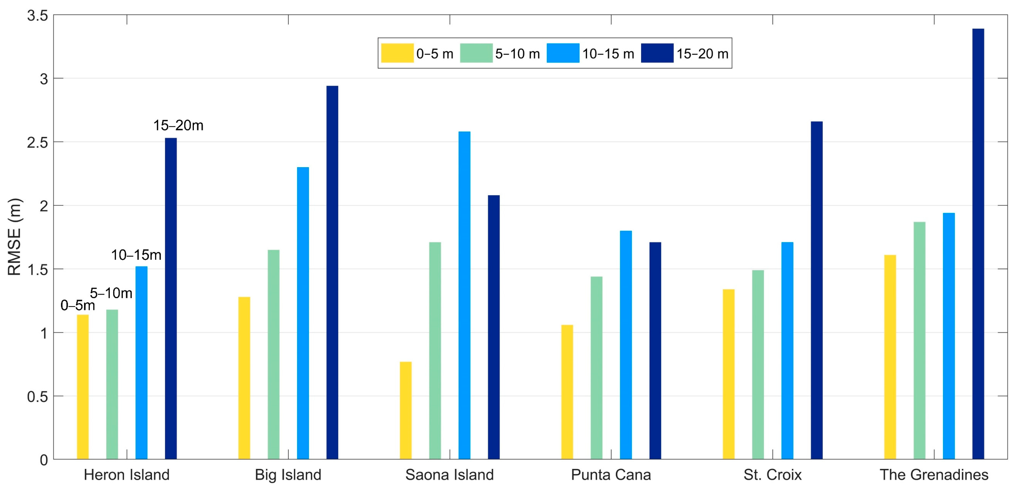
| RMSE (m) | Bias (m) | MNB | R2 | ||
|---|---|---|---|---|---|
| Heron, AU | 12-month mosaic | 1.35 | −0.38 | −0.18 | 0.98 |
| 6-month mosaic | 1.98 | −0.96 | −0.16 | 0.95 | |
| 3-month mosaic | 2.06 | −1.08 | −0.17 | 0.94 | |
| Big Island Hawaiʻi | 12-month mosaic | 1.98 | 0.30 | 0.03 | 0.85 |
| 6-month mosaic | 2.16 | 0.05 | −0.01 | 0.82 | |
| 3-month mosaic | 2.16 | 0.04 | −0.01 | 0.82 | |
| Saona Island, DR | 12-month mosaic | 1.83 | 1.09 | 0.13 | 0.78 |
| 6-month mosaic | 2.22 | 1.26 | 0.15 | 0.68 | |
| 3-month mosaic | 2.17 | 1.25 | 0.15 | 0.69 | |
| Punta Cana, DR | 12-month mosaic | 1.26 | 0.06 | −0.02 | 0.86 |
| 6-month mosaic | 1.56 | −0.20 | −0.10 | 0.78 | |
| 3-month mosaic | 1.57 | −0.21 | −0.10 | 0.78 | |
| St. Croix, USVI | 12-month mosaic | 1.60 | −0.02 | −0.03 | 0.79 |
| 6-month mosaic | 2.08 | 0.81 | 0.07 | 0.64 | |
| 3-month mosaic | 2.69 | 1.05 | 0.10 | 0.41 | |
| The Grenadines | 12-month mosaic | 1.92 | −0.83 | −0.15 | 0.81 |
| 6-month mosaic | 1.94 | −0.91 | −0.16 | 0.80 | |
| 3-month mosaic | 2.01 | −1.19 | −0.21 | 0.79 | |
Publisher’s Note: MDPI stays neutral with regard to jurisdictional claims in published maps and institutional affiliations. |
© 2021 by the authors. Licensee MDPI, Basel, Switzerland. This article is an open access article distributed under the terms and conditions of the Creative Commons Attribution (CC BY) license (https://creativecommons.org/licenses/by/4.0/).
Share and Cite
Li, J.; Knapp, D.E.; Lyons, M.; Roelfsema, C.; Phinn, S.; Schill, S.R.; Asner, G.P. Automated Global Shallow Water Bathymetry Mapping Using Google Earth Engine. Remote Sens. 2021, 13, 1469. https://doi.org/10.3390/rs13081469
Li J, Knapp DE, Lyons M, Roelfsema C, Phinn S, Schill SR, Asner GP. Automated Global Shallow Water Bathymetry Mapping Using Google Earth Engine. Remote Sensing. 2021; 13(8):1469. https://doi.org/10.3390/rs13081469
Chicago/Turabian StyleLi, Jiwei, David E. Knapp, Mitchell Lyons, Chris Roelfsema, Stuart Phinn, Steven R. Schill, and Gregory P. Asner. 2021. "Automated Global Shallow Water Bathymetry Mapping Using Google Earth Engine" Remote Sensing 13, no. 8: 1469. https://doi.org/10.3390/rs13081469
APA StyleLi, J., Knapp, D. E., Lyons, M., Roelfsema, C., Phinn, S., Schill, S. R., & Asner, G. P. (2021). Automated Global Shallow Water Bathymetry Mapping Using Google Earth Engine. Remote Sensing, 13(8), 1469. https://doi.org/10.3390/rs13081469