Article

Estimation of Photosynthetic and Non-Photosynthetic Vegetation Coverage in the Lower Reaches of Tarim River Based on Sentinel-2A Data

1
Xinjiang Institute of Ecology and Geography, Chinese Academy of Sciences, Urumqi 830011, China
2
University of Chinese Academy of Sciences, Beijing 100049, China
3
Research Center for Ecology and Environment of Central Asia, Chinese Academy of Sciences, Urumqi 830011, China
4
Sino-Belgian Joint Laboratory for Geo-Information, Xinjiang Institute of Ecology and Geography, Urumqi 830011, China
5
Department of Geography, Ghent University, 9000 Ghent, Belgium
6
Sino-Belgian Joint Laboratory for Geo-Information, Ghent University, 9000 Ghent, Belgium
7
Faculty of Environmental Sciences, Czech University of Life Sciences Prague, 16500 Prague, Czech Republic
*
Author to whom correspondence should be addressed.
Remote Sens. 2021, 13(8), 1458; https://doi.org/10.3390/rs13081458
Submission received: 18 February 2021 / Revised: 25 March 2021 / Accepted: 2 April 2021 / Published: 9 April 2021
(This article belongs to the Section Remote Sensing in Agriculture and Vegetation)

Abstract

:
Estimating the fractional coverage of the photosynthetic vegetation (fPV) and non-photosynthetic vegetation (fNPV) is essential for assessing the growth conditions of vegetation growth in arid areas and for monitoring environmental changes and desertification. The aim of this study was to estimate the fPV, fNPV and the fractional coverage of the bare soil (fBS) in the lower reaches of Tarim River quantitatively. The study acquired field data during September 2020 for obtaining the fPV, fNPV and fBS. Firstly, six photosynthetic vegetation indices (PVIs) and six non-photosynthetic vegetation indices (NPVIs) were calculated from Sentinel-2A image data. The PVIs include normalized difference vegetation index (NDVI), ratio vegetation index (RVI), soil adjusted vegetation index (SAVI), modified soil adjusted vegetation index (MSAVI), reduced simple ratio index (RSR) and global environment monitoring index (GEMI). Meanwhile, normalized difference index (NDI), normalized difference tillage index (NDTI), normalized difference senescent vegetation index (NDSVI), soil tillage index (STI), shortwave infrared ratio (SWIR32) and dead fuel index (DFI) constitutes the NPVIs. We then established linear regression model of different PVIs and fPV, and NPVIs and fNPV, respectively. Finally, we applied the GEMI-DFI model to analyze the spatial and seasonal variation of fPV and fNPV in the study area in 2020. The results showed that the GEMI and fPV revealed the best correlation coefficient (R2) of 0.59, while DFI and fNPV had the best correlation of R2 = 0.45. The accuracy of fPV, fNPV and fBS based on the determined PVIs and NPVIs as calculated by GEMI-DFI model are 0.69, 0.58 and 0.43, respectively. The fPV and fNPV are consistent with the vegetation phonological development characteristics in the study area. The study concluded that the application of the GEMI-DFI model in the fPV and fNPV estimation was sufficiently significant for monitoring the spatial and seasonal variation of vegetation and its ecological functions in arid areas.

1. Introduction

Vegetation cover is an important part of the ecosystem, which plays an important role in the soil and water conservation, restraining the desertification process, biodiversity protection and other ecological service and functions etc. [1,2]. From a functional point of view, vegetation can be divided into two parts: the photosynthetic vegetation (PV) and the non-photosynthetic vegetation (NPV) [3]. The PV mainly refers green leaves, while the NPV mainly includes the vegetation litter (dead leaves, dead branches and stems) and crop residues [4,5]. NPV is important as it not only affects the carbon storage, CO2 exchange capacity and temperature between the surface and soil [6,7] but also slows down soil erosion, increases the soil organic matter and improves the soil quality [8,9,10,11,12]. Therefore, an accurate estimation of the fractional coverage of the photosynthetic (fPV) and non-photosynthetic vegetation (fNPV) is of great significance in evaluating the ecological conditions.
In recent decades, remote sensing technology has made great progress in many aspects of geography [13,14]. In the fPV estimation, a number of indices (e.g. normalized difference vegetation index (NDVI) [15], soil adjusted vegetation index (SAVI) [16] and global environment monitoring index (GEMI) [17]) have been developed for PV utilizing spectral reflectance, which is widely used in various satellite platforms. Researchers have also proposed some vegetation indices so as to estimate the fNPV [18,19,20,21,22,23]. According to the spectral resolution of remote sensing data, non-photosynthetic vegetation indices (NPVIs) can be divided into hyperspectral NPVIs and multispectral NPVIs. Daughty [21] proposed hyperspectral NPVI (cellulose absorption index (CAI)) based on hyperspectral reflection characteristics of the NPV. Taking into account the limitations of hyperspectral data, researchers have developed many multispectral NPVIs using Landsat TM bands, such as the normalized difference index (NDI), the normalized difference tillage index (NDTI), the normalized difference senescent vegetation index (NDSVI) and the soil tillage index (STI). Guerschman [3] developed the shortwave infrared ratio index (SWIR32) based on MODIS data, which accurately estimated the fNPV of grasslands in Australia. Cao [24] utilized multispectral, MODIS, data to estimate NPV using the dead fuel index (DFI).
In order to estimate the proportion of PV and NPV in a pixel, based on spectral mixture analysis (SMA), researchers construct pixel unmixed model by using PVI and NPVI to estimate fPV and fNPV. And based on this, Guerschman [3] used the Hyperion data to propose pixel linear unmixed model of the NDVI-CAI (NDVI represents the PV, CAI represents the NPV). This updated methodology includes a better estimation of the spatiotemporal distribution of the PV and NPV in the sparse grasslands of Australia. Validating this methodology, Wang [25] applied the DFI index to construct the NDVI-DFI linear unmixed model based on the MOD09GHK surface reflectance data and effectively calculated the fPV and fNPV of the Xilingol grasslands. The foundational work mentioned above successfully showed suitable PV and NPV estimation using multispectral data but were limited in geographic and ecological scope. Focusing primarily on grasslands, other regions have not been explored yet. This work aims to estimate fPV and fNPV in riparian regions.
The Tarim River is a typical arid inland river basin. Due to the impact of human reclamation and irrigation in the upper reaches of the Tarim River, the water of the lower reaches has dropped sharply over the past 20 years, the Tetima Lake has dried up and the vegetation environment has deteriorated year by year. A comprehensive assessment of the vegetation changes in this area has been an ongoing effort. Some of the work, by Guli [26] and Li [27] employed a variety of models to discuss the suitability of the estimated vegetation coverage in the Tarim River Basin. Zhu [28] applied the method of transfer learning so as to extract and analyze the vegetation coverage changes in a long time series. These studies neglect to include NPV data in their analyses and rely largely on course resolution imagery, resulting in limited accuracy and uncertainty in the original estimations. Considering the improvements made to spectral instruments and the requirements for time and spatial resolution, Sentinel-2 satellite data are a good choice, specifically the multispectral imager (MSI) onboard could provide multispectral data with spatial resolution of 10 m and revisiting period of five days. Therefore, using the Sentinel-2 data with a high spatial and temporal resolution will be the focus to estimate the fPV and fNPV in the study area.
The objective of this study was to quantitatively estimate the seasonal variation in the fPV, fNPV and the fractional coverage of bare soil (fBS)in the lower reaches of the Tarim River based on Sentinel-2A image data. The study is divided into the following sections: (1) select the best PVI and NPVI as estimation index of fPV and fNPV according to the correlation coefficient of the PVIs with fPV and NPVIs with fNPV by linear regression models analysis, (2) build pixel unmixing model based on Sentinel-2A image data and quantitatively evaluate the results of estimating fPV and fNPV by using field sampled data and (3) map different periods of fPV, fNPV and fBS for the lower reaches of the Tarim River and analyze seasonal variation.

2. Materials and Methods

2.1. Study Area

The study area was located between the Dashkol Reservoir and Tetima Lake [39.5–40.59° N, 87.56–88.46° E] in the lower reaches of the Tarim River (Figure 1), which was surrounded by the Taklamakan Desert in the west and the Kuruktagh Desert in the northeast [29]. The study area’s annual precipitation ranged from 20 to 50 mm but the annual potential evaporation varied from 2500 to 3000 mm [30,31]. The total annual solar radiation varied in a range of 5692–6360 MJ m−2 with an annual sunshine from 2780 to 2980 h [32]. The water supply of the vegetation in the area mainly depended on the water streamed from the upper reaches of the river. The vegetation was mostly distributed on the floodplain on the riverbank, which composed of trees, shrubs and herbs. Dominant trees included the Populus euphratica, Elaeagnus angustifolia, the shrubs consisted of the Tamarix ramosissima, Lycium ruthenicum, Halimodendron halodendron, and herbs Phragmites australis, Alhagi sparsifolia, Poacynum hendersonii, Karelinia caspia [2].

2.2. Datasets

2.2.1. Field Data

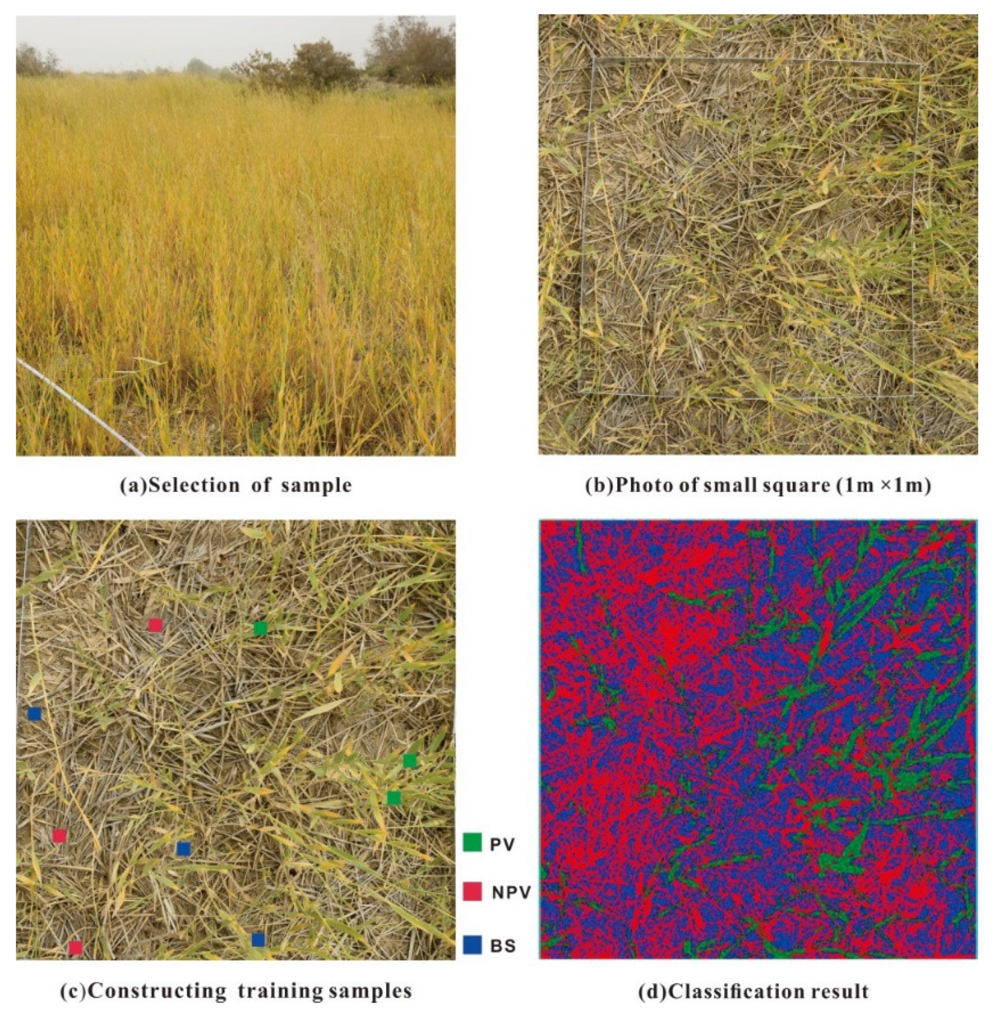
The fractional coverage samples of the PV, NPV and bare soil (BS) were collected from the Dashkol Reservoir, Gancaochang, Bozkol, Arghan, Kurgan and Tetima Lake. All samples were collected from 25 September to 29 September 2020 when the PV, NPV and BS existed simultaneously. Data collection and processing steps were as follows: we defined 10 m × 10 m squares, aligned to the north, and covered by a homogeneous vegetation distribution. The four corners and the center of the square were precisely located with GPS. Secondly, a smaller square of 1 m × 1 m was positioned randomly 3–5 times in the larger square. At the same time, a digital camera was used to take pictures vertically 1.6 m above the sample square. Each image was processed in ENVI 5.3. Photos were divided into NPV, PV and BS categories and training samples were established for each for supervised classification. Finally, we calculate the fPV, fNPV and fBS of all 1 m × 1 m squares in each 10 m × 10 m square, and count the average value to represent the fPV, fNPV and fBS in the 10 m × 10 m square. Figure 2 shows the field square acquisition and classification processing.

2.2.2. Remote Sensing Data

Sentinel-2A Level-1C data was used in this study. Images were from, seven periods on 5 April, 25 May, 24 July, 18 August, 12 September, 2 October and 6 November 2020. The data were radiometrically calibrated and geometrically corrected, downloaded from the ESA website (https://sci hub.copernicus.eu/home). The image preprocessing was carried out in SNAP 6.0 provided by ESA (Sentinel application platform) and the ENVI 5.3 software platform. The SNAP 6.0 Sen2Cor (Sentinel to Correction) plug-in was used to perform atmospheric correction processing on all L1C data, which resulted in 9 bands (Band 2, Band 3, Band 4, Band 5, Band 6, Band 7. Band 8a, Band 11 and Band 12) L2A surface reflectance data. And the 9-band data were combined into a single multiple image using composite bands in Quantum GIS (QGIS) and then resampled to 10 m pixels. Image data were mosaicked, and the study area was clipped. Water features were masked by using the modified normalized difference water index (MNDWI) combined with the threshold method (threshold value is −0.08).

2.3. Methods

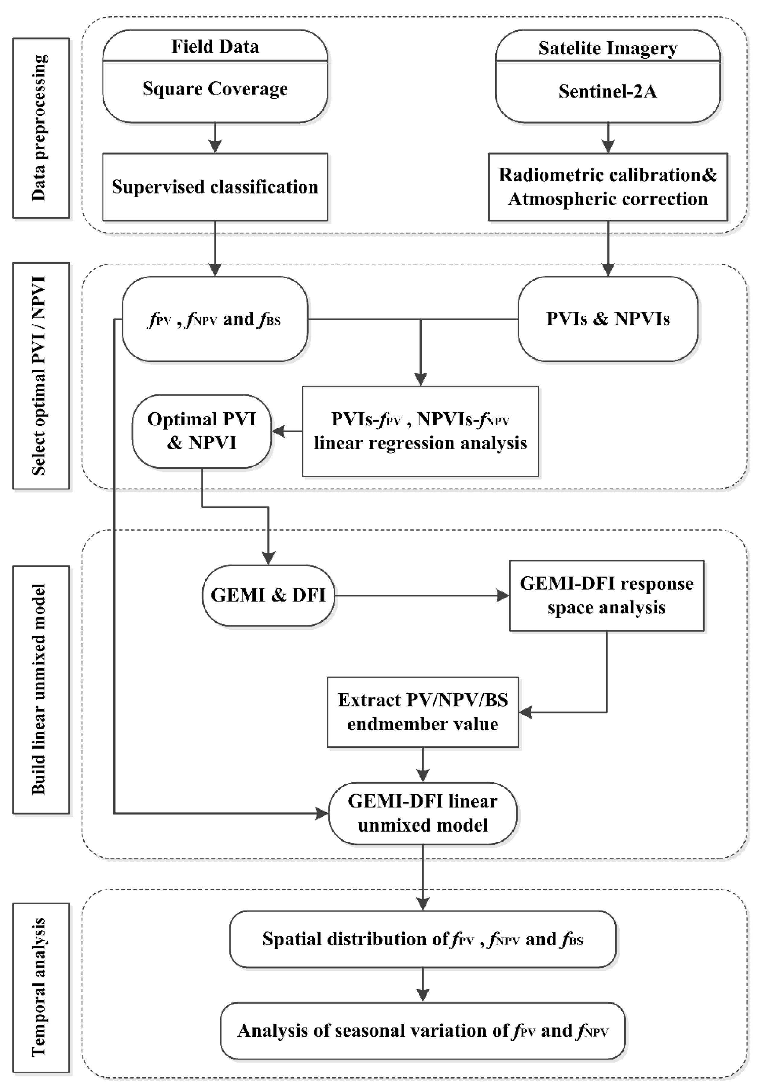
The general workflow of this project was: (1) construct linear regression models of the PVIs and fPV, NPVIs and fNPV, respectively, to select the optimal PVIs and NPVIs, (2) analyze the feasibility of the selected PVIs and NPVIs so as to construct the response space, (3) apply the pixel linear unmixed model to determine the end member values of the PV, NPV and BS based on the Sentinel-2A image data, (4) quantitatively evaluate the estimation accuracy of the fPV and fNPV using the field sampled data, (5) map time series of the fPV, fNPV and fBS for the lower reaches of the Tarim River and to analyze the seasonal variation. The flowchart is shown in Figure 3.

2.3.1. PVIs and NPVIs

PV was affected by chlorophyll and the cell structure and showed typical spectral characteristics of green vegetation, with obvious peaks and valleys [25]. In this study, we selected several PVIs for testing, including the NDVI [33], RVI [34], SAVI [35], MSAVI [16], RSR [36] and GEMI [17] (Table 1).
NPV and BS had similar spectral reflectance characteristics in Visible and Near Infrared band and but could be differentiated using the Shortwave Infrared band (1600 nm and 2100 nm) [25]. In this study, we selected several PVIs for testing, including the NDI [23], NDTI [19], NDSAVI [20], STI [19], SWIR32 [3] and DFI [24] (Table 2).
PVIs and NPVIs were calculated using ArcGIS 10.5 software. The PVI value and fPV measured value, and NPVI value and fNPV measured value, were constructed linear regression models of PVI and NPVI relative to fPV and fNPV, respectively, and were used to evaluate the accuracy of the various indices. Considering the number of samples we have taken, we used the leave-one-out cross-validation (LOOCV) which was suitable for a small number of sample. In LOOCV, each sample was excluded in turn and the regression model was calculated with all the remnants samples and used to predict that sample. The benefit of LOOCV was its aptitude to detect outliers and its capability of providing nearly unbiased estimations of the prediction error [4,37]. The performance of these models was assessed by the coefficients of determination (R2), root mean square error of leave-one-out cross-validation (RMSECV) and regression significance (p):
R 2 = i = 1 n ( x i x ¯ ) ( y i y ¯ ) i = 1 n ( x i x ¯ ) 2 i = 1 n ( y i y ¯ ) 2
R M S E C V = 1 n i = 1 n ( x i y i ) 2
where n shows the sample plots’ number, xi is the measured value of the sample plot i, yi stands for the estimated value of the sample plot i, x ¯ illustrates the mean value of the measured sample plots, y ¯ stipulates the mean value of the estimated sample plots.

2.3.2. Linear Unmixed Model

Guerschman [3] hypothesized that the NDVI and CAI could resolve the fractions of the PV, NPV and BS, when the NDVI and fPV were linearly related (as were the CAI and fNPV). This situation is reflected in the scatterplot of the NDVI and CAI, namely that the feature space forms a triangle; BS is situated on the right side of the triangle, with a high NDVI and intermediate CAI value; the NPV is located in the upper left corner of the triangle, showing a low NDVI and a high CAI value; the BS is seen in the lower left corner of the triangle, having low NDVI and CAI values; Cao [24] used the DFI (replacing CAI) to present the NPV in order to construct the NDVI-DFI linear unmixed model, and it is successful in estimating the fractions of the PV, NPV and BS. Therefore, we applied the GEMI-DFI linear unmixed model to assess the fractions of the PV, NPV and BS in the study area (Figure 4).
PV is expressed by the global environmental monitoring index (GEMI) and the NPV by the dead fuel index (DFI), The GEMI formula is calculated as Table 1, The DFI formula is the following in Table 2. The relative proportions of each fractional coverage for any Sentinel-2A image pixel were found by solving the equations:
G S = [ f i G i ] = [ f PV G PV + f NPV G NPV + f BS G BS ]
D S = [ f i D i ] = [ f PV D PV + f NPV D NPV + f BS D BS ]
f i = [ f PV + f NPV + f BS ] = 1
where GS and DS show the GEMI and DFI value in the given Sentinel-2A image pixel, the fPV, fNPV and fBS illustrate the fractional coverage of the PV, NPV and BS; the GPV, GNPV and GBS are the GEMI values of the end members, the DPV, DNPV and DBS demonstrate the DFI values of the end members. It forces the values of fPV, fNPV and fBS to sum to unity. If the sum does not get one, the pixel has a negative or higher than 1 value in at least one end member. When that occurred, the following correction was applied:
C x = 0 ( 0.2 < C x < 0 )
C x = 1 ( 1 < C x < 1.2 )
C y = C y / ( C y + C z )
C z = C z / ( C y + C z )
where Cx is the value not within a specified range (Cx < −0.2 or Cx > 1.2), and Cy and Cz are the values of the other two end members. If the range of Cx is amounts from −0.2 to 0, Cx is 0; if the range of Cx is 1 to 1.2, Cx is 1; the condition is mentioned in the above two cases, we only calculated Cy and Cz.

2.3.3. Determination of the GEMI and DFI End Member Value

The choice of pure end members was the key to success of the PV and NPV model inversion. The GEMI-DFI linear unmixed model needed to become a pure end member of the PV, NPV and BS to calculate the corresponding proper values and the model needed be used to solve the fractional coverage of each end member. We employed the pixel purity index (PPI) method to determine the pure end member. Firstly, the Sentinel-2A images were subjected to the minimum noise fraction (MNF) so as to reduce the image dimensionality during different periods. The first 6 bands of each image period were selected for calculation and the number of iterations was set to 5000 in order to generate the PPI. Secondly, the GEMI and DFI were calculated for various period images. Finally, the pixels near the vertices of the triangular feature space were regarded as pure pixels.

2.3.4. Model Evaluation

In order to quantitatively evaluate the performance of the model’s estimation ability, the coefficients of determination (R2), root mean square error (RMSE) and mean error (ME) were applied.
R M S E = 1 n i = 1 n ( x i y i ) 2
M E = 1 n i = 1 n ( x i y i )
where n shows the sample plots’ number, xi is the measured value of the sample plot i, yi stands for the estimated value of the sample plot i.

3. Results

3.1. PVI and NPVI Index Optimization

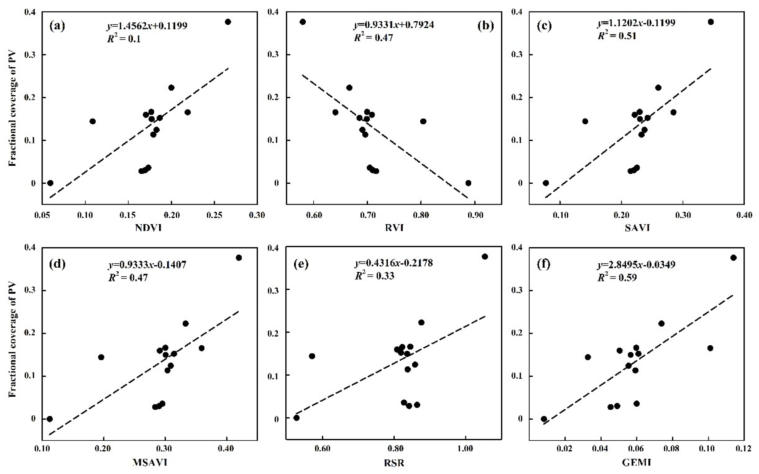
In this study, six PV indices (NDVI, RVI, SAVI, MSAVI, RSR and GEMI) were selected to build linear regression models with fPV (Table 3 and Figure 5). Various PVIs exhibited different performance, with the R2 ranging from 0.33 to 0.59 and the RMSECV ranging from 0.752 to 0.1283. The GEMI index showed the highest correlation, with the R2 reaching 0.59 and RMSECV being 0.752 (p < 0.05). The RVI, MSAVI and RSR indices had low correlations (all R2 lower than 0.50 and RMSECV higher than 0.8). The GEMI index was used as the PVI index to estimate the fPV of the study area. In order to count the GEMI value, the GEMI index value had been normalized.
We selected six NPVI indices (NDI, NDTI, NDSAVI, DFI, STI and SWIR32) to construct linear regression models with the fNPV (Table 4 and Figure 6). Compared with the correlation between the PVI indices and fPV, the correlation between the NPVIs and fNPV was lower. This might be caused by similar spectral characteristics of the NPV and BS [24]. The DFI index showed the best performance with a R2 of 0.45 and RMSECV of 0.2111(p < 0.05). The STI, NDTI, SWIR32, NDSVI and NDI indices were lower than the DFI, with the R2 ranging from 0.02 to 0.43, and the RMSECV from 0.2611 to 0.2627. Therefore, the DFI index was selected to assess the fNPV of the study area.

3.2. The Feasibility of the GEMI-DFI Model

We obtained the GEMI-DFI response space by calculating the GEMI and DFI values for seven Sentinel-2A images’ data (Figure 7). GEMI-DFI response space of the first six images was basically triangular, which was consistent with the theoretical conceptual mode. It showed that the GEMI-DFI linear unmixed model could be utilized to estimate the fractional coverage of the PV, NPV and BS. The last GEMI-DFI response space image did not seem to conform to the triangle shape. We selected images covering the growing season from spring to fall (April to November) and as vegetation leafed out and became active, GEMI values increased while DFI values declined. The inverse was seen with the onset of fall, as vegetation began to senesce and go dormant.

3.3. Evaluation of the fPV and fNPV Estimation Accuracy

Considering that field data collection occurred between 25–29 September in 2020, Sentinel 2A data collected on 2 October in 2020 were selected. We used the GEMI-DFI linear unmixed model (combined with the PPI) to obtain the spatial distribution of the fPV, fNPV and fBS. The BS proportion in the study area was the largest and the PV and NPV were mainly distributed along the downstream river and the Tetima Lake. In order to clearly show the model result in estimating the fPV and fNPV, we selected the areas with a vegetation distribution evenly for display. The four regions were: a (Dashkol), b (Chiwinkol), c (Bozkol) and d (Tetima Lake). The fNPV of the four regions was greater than the fPV, indicating that after October, the vegetation entered the end of the growing season and the increase in the NPV (during this period) caused an increase in the proportion of the fNPV (Figure 8) in turn.
We could conclude from Figure 9 that the estimated fPV has the best correlation with the measured fPV, with a R2 of 0.69 and RMSE of 0.07 (p < 0.05). The estimated fNPV and the measured fNPV have a lower correlation with a R2 of 0.58 and RMSE of 0.17 (p < 0.05). For BS, the measured (and estimated) values possess the lowest correlation, with a R2 of 0.43 and a RMSE of 0.17 (p < 0.05). For the PV, the fitted line is situated below the reference line (1:1 line) and the ME value amounts to −2.67%. The data mentioned above show that overall the estimated fPV value is lower than the measured fPV value, this is due to the fact that the acquisition time of the Sentinel-2A image data is later than the one for the field measured data, resulting in lower fPV estimates. Concerning the fNPV, the value of ME is 3.14%, this means that the estimated fPV value is higher than the measured fPV value. In general, the estimation accuracy of the fNPV and fBS is lower than the fPV, this reflects the fact that the PV could be resolved in an easier way than the NPV. Both the NPV and BS have similar spectral reflectance characteristics, resulting in a greater probability of wrong classification between the NPV and BS.

3.4. Seasonal Variation of the fPV and fNPV

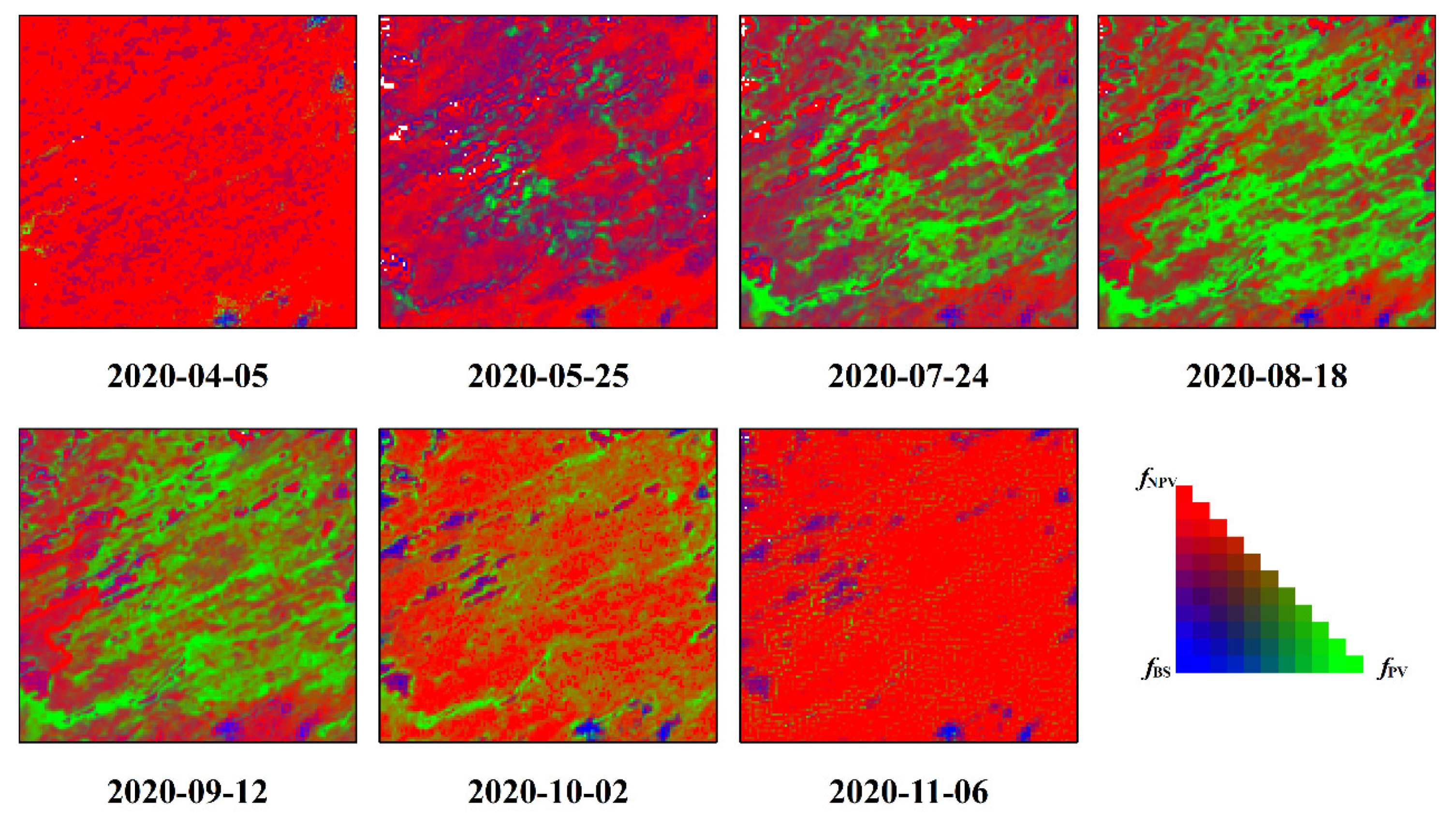
In this study, the b region was chosen as the representative area for seasonal variation. This was located in the Chiwinkol wetland, which was less disturbed by human activities and could have better indicated the natural alternation of the PV and NPV’s seasonal variation. We selected Sentinel-2A image data from seven periods and used the GEMI-DFI linear unmixed model to estimate the fPV, fNPV and fBS during different periods (Figure 10). We counted mean values of the fPV, fNPV and fBS in the b region (Figure 11). By analyzing the changes of the fPV, fNPV and fBS values, it was found that the seasonal variation of the fPV and fNPV was estimated by the GEMI-DFI model in conformity with the characteristics of the vegetation phenology. In April, most of the vegetation not yet broken dormancy and as such, there was a large NPV amount, the GEMI value was low, the DFI value was high, the fNPV was 0.93 and the fPV measured 0.01. In May, as the vegetation had emerged and begun actively growing, the GEMI value increased, the DFI value decreased, the fPV rose to 0.17 and the fNPV declined to 0.69. As the growing season progressed, GEMI increased, peaking in August with DFI following an inverse trend, and the DFI value fell to the lowest point. Similarly, fPV reached maximum value, which was 0.44 and fNPV its lowest value of 0.45. In September, the vegetation began to yellow and GEMI fell and DFI rose. By the beginning of October, most of the vegetation had already withered, the fNPV occupied the dominant position again (at 0.81) and the fPV decreased further to 0.17. The fBS value remained in a relatively stable position throughout the whole year.

4. Discussion

This study explored the performance of several Sentinel-2A based PVIs by constructing linear regression models in the lower reaches of the Tarim River. The GEMI index has the best correlation with the fPV, which is consistent with the conclusion of Liu [38] on the vegetation information monitoring this area. The GEMI index shows greater advantages in detecting the low coverage vegetation information. In the regression analysis between the NPVI index and fNPV, the correlation between the DFI index and fNPV is better than for those of the NDI, NDTI, NDSVI, STI and SWIR32. Among them, the NDI and NDSVI indices mainly use Band 11 (SWIR1: 1565~1655 nm), combined with a visible light band (NDI for the NIR band, NDSVI for the Red band) and without combining Band 12 (SWIR: 2100~2280 nm). Previous research has demonstrated that the cellulose absorption signature (amounting to around 2100 nm in the SWIR region) has a strong discriminatory ability between the NPV, PV and BS [8]; so Band 12 is a good choice to distinguish the PV, NPV and BS. Compared with the DFI index, STI and SWIR32 simply perform ratio calculations. The DFI index uses more bands for the calculation, including the Red, NIR SWIR1 and SWIR2. It might reduce the impact of the BS background to some extent and it might further improve NPV detection [4]. Ji [39] similarly concluded that the red-edge and NIR bands of the Sentinel-2 data are effective in improving the accuracy of the fNPV estimates. The manner in which the red-edge band of the Sentinel-2 data could be utilized in order to estimate the vegetation information accurately still need further exploration.
The study uses the PPI method to extract the pure end members of the image data, which eliminates the discrepancies between the image data and the measured data, ensuring that both have the same spatial scale, which is widely employed to select the pure end of the spectrum [14,37]. We were able to estimate the fPV and fNPV of the study area in different periods by means of the GEMI-DFI model, revealing the changes in the photosynthetic and non-photosynthetic vegetation at different growth stages. The NPV proportion is greater at the beginning and at the end of the growing season, while the proportion of the PV peaks in the middle of the vegetation growing season. This is consistent with the findings of Wang [40] estimating the fPV and fNPV in the typical grasslands of Xilingol, indicating that the GEMI-DFI model is feasible to estimate the fPV and fNPV in the lower reaches of the Tarim River. The accuracy of the fNPV estimation (R2 = 0.58) is slightly lower than for the fPV estimation (R2 = 0.69). As the NPV and BS have similar spectral reflection characteristics in the visible band [3,41], the NPV estimation is more susceptible to the influence of the BS background, which could lead to a false distinction between the NPV and BS. Both the GEMI and DFI values are influenced by a variety of factors, such as the vegetation type, vegetation structure, etc. [17,24]. Therefore, more consideration should be given to the influencing factors in future studies on the PV and NPV.
The overall vegetation coverage in the study area is low, as vegetation is mostly distributed along the watercourses. Due to this, higher spatial resolution imagery is required to obtain more detailed information on the type of the vegetation [42]. Based on this, the Sentinel-2A data with a resolution of 10 m were used, which might reduce the spatial heterogeneity of the mixed pixels and improve the estimation accuracy by a better acquisition of pure pixels. There is still some uncertainty noticeable in the estimation of the PV, NPV and BS using multispectral data. In fact, the vegetation and other surrounding components form a complex system [37] and it endures stages of greening, heading, flowering, maturing and yellowing [43]. The above-mentioned conditions affect the acquisition of the estimated GEMI and DFI values, thereby impacting the model’s accuracy to estimate the fPV, fNPV and fBS. In addition, uncertain factors also exist in the field data collection. The moment in which the photo was taken does not match the time of the satellite transit; the visual interpretation of the PV, NPV and BS classification and the accuracy of the geometric alignment will inevitably be influenced by subjective factors, resulting in errors in the fPV, fNPV and fBS estimates [18]. This study relies on the coverage obtained from field sampled data as the verification data. Taking into account the diversity of vegetation types and structures, the spectral characteristics of vegetation are different. We should combine spectral data to accurately estimate the changing trends of different types of vegetation. The use of drones is also an effective measure to improve the estimation of vegetation coverage. This method can obtain a large area of vegetation coverage and reduce the error of its estimation and should be taken into account in future research work.

5. Conclusions

In this study, we constructed the GEMI-DFI linear unmixed model based on the Sentinel-2A image data so as to estimate the fractional coverage of the PV, NPV and BS in the lower reaches of the Tarim River combined with the field measured data for an accuracy evaluation. The main conclusions are as follows:
We established a linear regression model for the PVIs and fPV, and NPVIs and fNPV. The study found that the GEMI have a significantly linear correlation with the fPV, R2 is 0.59 and the DFI has a significantly linear correlation with the fNPV, R2 measuring 0.45. We used GEMI and DFI indices to construct linear unmixed model, the response space shown as triangle, which conformed the basic assumption of the linear unmixed model.
The GEMI-DFI linear unmixed models could effectively estimate the fPV and fNPV, but the accuracy of estimation fPV is higher than that of fNPV. How to improve the accuracy of estimation of fNPV is the focus of future work.
Considering the number of sampling data, we need to collect more vegetation coverage data in future work. We can use drones as a platform for obtaining vegetation coverage to achieve a wide range of coverage, thereby improving the accuracy of fPV, fNPV and fBS estimation.

Author Contributions

Conceptualization, A.K.; methodology, Z.G.; software, A.K.; validation, Z.G., A.A. and A.K.; resources, A.K.; data curation, Z.G. and S.W.; writing—original draft preparation, Z.G.; writing—review and editing, Z.G., A.K., T.V.d.V., H.A., P.D.M. and E.D.U.; visualization, Z.G.; supervision, A.K.; project administration, A.K.; funding acquisition, A.K. All authors have read and agreed to the published version of the manuscript.

Funding

This research was funded by the National Natural Science Foundation of China (grant number 32071655; 31570536). Chinese Academy of Sciences President’s International Fellowship Initiative (PIFI, Grant No. 2021VCA0004, 2017VCA0002).

Acknowledgments

The authors would like to thank ESA (https://scihub.copernicus.eu/ (accessed on 2 April 2021)) for providing Sentinel-2A data for this study. Thanks to Management Bureau of the Tarim River Main Stream for providing support for field work, especially Shengwu Xu and Salamu Ayoufu. Thanks to all the editors and reviewers for their meaningful comments so that we can improve the quality of this manuscript in different aspects.

Conflicts of Interest

The authors declare no conflict of interest.

References

  1. Novillo, C.; Arrogante-Funes, P.; Romero-Calcerrada, R. Recent NDVI Trends in Mainland Spain: Land-Cover and Phytoclimatic-Type Implications. ISPRS Int. J. Geo. Inf. 2019, 8, 43. [Google Scholar] [CrossRef] [Green Version]
  2. Xu, H.; Ye, M.; Song, Y.; Chen, Y. The natural vegetation responses to the groundwater change resulting from ecological water conveyances to the lower Tarim River. Environ. Monit. Assess. 2007, 131, 37–48. [Google Scholar] [CrossRef]
  3. Guerschman, J.P.; Hill, M.J.; Renzullo, L.J.; Barrett, D.J.; Marks, A.S.; Botha, E.J. Estimating fractional cover of photosynthetic vegetation, non-photosynthetic vegetation and bare soil in the Australian tropical savanna region upscaling the EO-1 Hyperion and MODIS sensors. Remote Sens. Environ. 2009, 113, 928–945. [Google Scholar] [CrossRef]
  4. Chai, G.; Wang, J.; Wang, G.; Kang, L.; Wu, M.; Wang, Z. Estimating fractional cover of non-photosynthetic vegetation in a typical grassland area of northern China based on Moderate Resolution Imaging Spectroradiometer (MODIS) image data. Int. J. Remote Sens. 2019, 40, 8793–8810. [Google Scholar] [CrossRef]
  5. Li, Z.; Guo, X. Remote sensing of terrestrial non-photosynthetic vegetation using hyperspectral, multispectral, SAR, and LiDAR data. Prog. Phys. Geogr. Earth Environ. 2015, 40, 276–304. [Google Scholar] [CrossRef]
  6. Ren, H.; Zhou, G. Estimating senesced biomass of desert steppe in Inner Mongolia using field spectrometric data. Agric. For. Meteorol. 2012, 161, 66–71. [Google Scholar] [CrossRef]
  7. Facelli, J.M.; Pickett, S.T.A. Plant litter Its dynamics and effects on plant community structure. Bot. Rev. 1991, 57, 1–32. [Google Scholar] [CrossRef]
  8. Daughtry, C.S.T.; Hunt, E.R.; McMurtrey, J.E. Assessing crop residue cover using shortwave infrared reflectance. Remote Sens. Environ. 2004, 90, 126–134. [Google Scholar] [CrossRef]
  9. Wang, J.; Zhao, M.; Willms, W.D.; Han, G.; Wang, Z.; Bai, Y. Can plant litter affect net primary production of a typical steppe in Inner Mongolia? J. Veg. Sci. 2011, 22, 367–376. [Google Scholar] [CrossRef]
  10. Nagler, P.L.; Inoue, Y.; Glenn, E.P.; Russ, A.L.; Daughtry, C.S.T. Cellulose absorption index (CAI) to quantify mixed soil–plant litter scenes. Remote Sens. Environ. 2003, 87, 310–325. [Google Scholar] [CrossRef]
  11. Henry, H.A.L.; Brizgys, K.; Field, C.B. Litter Decomposition in a California Annual Grassland: Interactions Between Photodegradation and Litter Layer Thickness. Ecosystems 2008, 11, 545–554. [Google Scholar] [CrossRef]
  12. Daughtry, C.S.; Serbin, G.; Reeves, J.; Doraiswamy, P.; Hunt, E.R. Spectral Reflectance of Wheat Residue during Decomposition and Remotely Sensed Estimates of Residue Cover. Remote Sens. 2010, 2, 416–431. [Google Scholar] [CrossRef] [Green Version]
  13. Wu, S.; Gao, X.; Lei, J.; Zhou, N.; Wang, Y. Spatial and Temporal Changes in the Normalized Difference Vegetation Index and Their Driving Factors in the Desert/Grassland Biome Transition Zone of the Sahel Region of Africa. Remote Sens. 2020, 12, 4119. [Google Scholar] [CrossRef]
  14. Chai, G.; Wang, J.; Wu, M.; Li, G.; Zhang, L.; Wang, Z. Mapping the fractional cover of non-photosynthetic vegetation and its spatiotemporal variations in the Xilingol grassland using MODIS imagery (2000–2019). Geocarto Int. 2020, 1–17. [Google Scholar] [CrossRef]
  15. de Jong, R.; de Bruin, S.; de Wit, A.; Schaepman, M.E.; Dent, D.L. Analysis of monotonic greening and browning trends from global NDVI time-series. Remote Sens. Environ. 2011, 115, 692–702. [Google Scholar] [CrossRef] [Green Version]
  16. Qi, J.; Chehbouni, A.; Huete, A.R.; Kerr, Y.H.; Sorooshian, S. A modified soil adjusted vegetation index. Remote Sens. Environ. 1994, 48, 119–126. [Google Scholar] [CrossRef]
  17. Pinty, B.; Verstraete, M.M. GEMI: A non-linear index to monitor global vegetation from satellites. Vegetatio 1992, 101, 15–20. [Google Scholar] [CrossRef]
  18. Numata, I.; Roberts, D.; Chadwick, O.; Schimel, J.; Galvao, L.; Soares, J. Evaluation of hyperspectral data for pasture estimate in the Brazilian Amazon using field and imaging spectrometers. Remote Sens. Environ. 2008, 112, 1569–1583. [Google Scholar] [CrossRef]
  19. Deventer, V.; Ward, A.; Gowda, P.; Lyon, J. Using Thematic Mapper Data to Identify Contrasting Soil Plains and Tillage Practices. Photogramm. Eng. Remote Sens. 1997, 63, 87–93. [Google Scholar] [CrossRef]
  20. Qi, J.; Marsett, R.; Heilman, P.; Biedenbender, S.; Moran, S.; Goodrich, D. RANGES improve satellite-based information and land cover assessments in southwest United States. Eos Trans. Am. Geophys. Union 2002, 83, 601–605. [Google Scholar] [CrossRef]
  21. Daughtry, C.; McMurtrey, J., III; Nagler, P.; Kim, M.; Chappelle, E. Spectral reflectance of soils and crop residues. In Near Infrared Spectroscopy: The Future Waves; Nir Publications: Chichester, UK, 1996; pp. 505–510. [Google Scholar]
  22. Biard, F.; Bannari, A.; Bonn, F. SACRI (Soil Adjusted Corn Residue Index): An index using near and mid-infrared for the detection of residues of maize. In Proceedings of the 17th Canadian Symposium on Remote Sensing, Saskatoon, SK, Canada, 13–15 June 1995; pp. 417–423. [Google Scholar]
  23. McNairn, H.; Protz, R. Mapping Corn Residue Cover on Agricultural Fields in Oxford County, Ontario, Using Thematic Mapper. Can. J. Remote Sens. 1993, 19, 152–159. [Google Scholar] [CrossRef]
  24. Cao, X.; Chen, J.; Matsushita, B.; Imura, H. Developing a MODIS-based index to discriminate dead fuel from photosynthetic vegetation and soil background in the Asian steppe area. Int. J. Remote Sens. 2010, 31, 1589–1604. [Google Scholar] [CrossRef]
  25. Guangzhen, W. Estimating Fractional Cover of Photosynthetic/Non-Photosynthetic Vegetation in the Xilingol Typical Grassland Region with Remote Sensing Data. Master’s Thesis, Ludong University, Yaitai, China, 2018. [Google Scholar]
  26. Jiapaer, G.; Xi, C.; Anming, B. Coverage ectraction and up-scaling of sparse desert vegetation in arid. Chin. J. Appl. Ecol. 2009, 20, 2925–2934. [Google Scholar]
  27. Xiangting, L.; Jie, B.; Guanglu, L.; Geping, L.; Jiapaer, G.; Junli, L. Comparison of methods based on MODIS for estimating sparse vegetation fraction across desert in Xinjiang. Arid Land Geogr. 2013, 36, 502–511. [Google Scholar]
  28. Changming, Z.; Junli, L.; Zhanfeng, S.; Qian, S. Satiotemporal dynamics of vegetation activities in the lower reach of the TarimRiver based on MODIS intensive time series data. Resour. Sci. 2019, 41, 591–600. [Google Scholar]
  29. Liu, G.; Kurban, A.; Duan, H.; Halik, U.; Ablekim, A.; Zhang, L. Desert riparian forest colonization in the lower reaches of Tarim River based on remote sensing analysis. Environ. Earth Sci. 2013, 71, 4579–4589. [Google Scholar] [CrossRef]
  30. Chen, Y.; Chen, Y.; Xu, C.; Ye, Z.; Li, Z.; Zhu, C.; Ma, X. Effects of ecological water conveyance on groundwater dynamics and riparian vegetation in the lower reaches of Tarim River, China. Hydrol. Process. Int. J. 2009, 24, 170–177. [Google Scholar] [CrossRef]
  31. Xu, J.; Chen, Y.; Li, W.; Zhang, L.; Hong, Y.; Bi, X.; Yang, Y. Statistical analysis of groundwater chemistry of the Tarim River lower reaches, Northwest China. Environ. Earth Sci. 2011, 65, 1807–1820. [Google Scholar] [CrossRef]
  32. Chen, Y.; Chen, Y.; Xu, C.; Li, W. Groundwater depth affects the daily course of gas exchange parameters of Populus euphratica in arid areas. Environ. Earth Sci. 2012, 66, 433–440. [Google Scholar] [CrossRef]
  33. Deering, D.W. Rangeland Reflectance Characteristics Measured by Aircraft and Spacecraft Sensors. Ph.D. Thesis, Texas A&M University, College Station, TX, USA, 1978; 338p. [Google Scholar]
  34. Jordan, C.F. Derivation of leaf-area index from quality of light on the forest floor. Ecology 1969, 50, 663–666. [Google Scholar] [CrossRef]
  35. Huete, A.R. A soil-adjusted vegetation index (SAVI). Remote Sens. Environ. 1988, 25, 295–309. [Google Scholar] [CrossRef]
  36. Brown, L.; Chen, J.M.; Leblanc, S.G.; Cihlar, J. A Shortwave Infrared Modification to the Simple Ratio for LAI Retrieval in Boreal Forests: An Image and Model Analysis. Remote Sens. Environ. 2000, 71, 16–25. [Google Scholar] [CrossRef]
  37. Schlerf, M.; Atzberger, C.; Hill, J. Remote sensing of forest biophysical variables using HyMap imaging spectrometer data. Remote Sens. Environ. 2005, 95, 177–194. [Google Scholar] [CrossRef] [Green Version]
  38. Guilin, L.; Luocheng, Z.; Guanyu, L. Sparse Desert Vegetation Extraction in Extreme Arid Region Based on Remote Sensing Imagery. J. Arid Land Resour. Environ. 2013, 27, 37–40. [Google Scholar]
  39. Ji, C.; Li, X.; Wei, H.; Li, S. Comparison of Different Multispectral Sensors for Photosynthetic and Non-Photosynthetic Vegetation-Fraction Retrieval. Remote Sens. 2020, 12, 115. [Google Scholar] [CrossRef] [Green Version]
  40. Wang, G.; Wang, J.; Zou, X.; Chai, G.; Wu, M.; Wang, Z. Estimating the fractional cover of photosynthetic vegetation, non-photosynthetic vegetation and bare soil from MODIS data: Assessing the applicability of the NDVI-DFI model in the typical Xilingol grasslands. Int. J. Appl. Earth Obs. Geoinf. 2019, 76, 154–166. [Google Scholar] [CrossRef]
  41. Daughtry, C.S.T.; Hunt, E.R.; Doraiswamy, P.C.; McMurtrey, J.E. Remote Sensing the Spatial Distribution of Crop Residues. Agron. J. 2005, 97, 864–871. [Google Scholar] [CrossRef]
  42. Guoqi, C.; Jingpu, W.; Xueyong, Z.; Guangzhen, W.; Liu, H.; Zhoulong, W. Estimating Fractional Cover of Photosynthetic /Non-Photosynthetic Vegetation in a Typical Steppe Region Based on Sentinel-2 Data. Pratacult. Sci. 2018, 35, 70–78. [Google Scholar]
  43. Bingru, Z.; Chuang, L.; Jingjie, W.; Wenbo, C. Spatial and Temporal Change of MODIS-NDVI in Xilinguole Ggrassland. Grassl. China 2004, 26, 2–9. [Google Scholar]
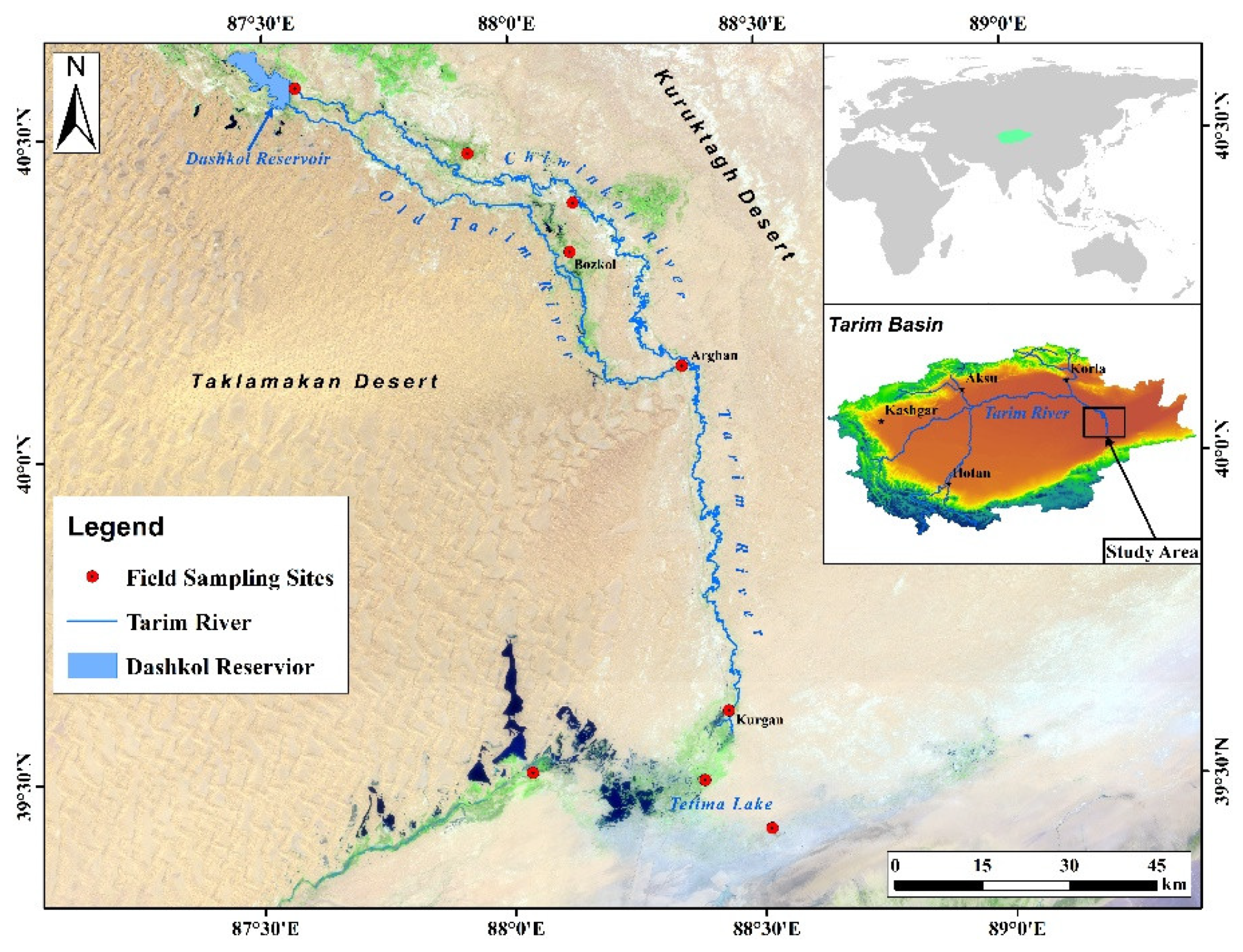
Figure 1. Location of the study area and distribution of the sample sites.
Remotesensing 13 01458 g001
Figure 2. Field square acquisition and classification processing.
Remotesensing 13 01458 g002
Figure 3. A methodology flowchart.
Remotesensing 13 01458 g003
Figure 4. The conceptual model of the global environment monitoring index and cellulose absorption index (GEMI-CAI) relation triangle of the PV, NPV and BS.
Remotesensing 13 01458 g004
Figure 5. Linear regression between different PVIs and the fPV. The PVIs are (a) NDVI, (b) RVI, (c) SAVI, (d) MSAVI, (e) RSR and (f) GEMI, respectively.
Remotesensing 13 01458 g005
Figure 6. Linear regression between different NPVIs and the fNPV. The NPVIs are (a) NDI, (b) NDTI, (c) NDSVI, (d) DFI, (e) STI and (f) SWIR32, respectively.
Remotesensing 13 01458 g006
Figure 7. Response spaces of the Sentinel-2A reflectance spectral defined by the GEMI and DFI for seven dates in 2020. The green, red and blue circle indicate the position of the PV, NPV and BS end members, respectively (and form triangles). The colors indicate the point density from blue (low density) to dark red (high density). (a) 5 April 2020, (b) 25 May 2020, (c) 24 July 2020, (d) 18 August 2020, (e) 12 September 2020, (f) 2 October 2020, (g) 6 November 2020.
Remotesensing 13 01458 g007
Figure 8. Spatial distribution of the fPV, fNPV and fBS in the study area (based on the Sentinel-2A image). Four areas: a (Dashkol), b (Chiwinkol), c (Bozkol) and d (Tetima Lake). The proportions of the fractional coverage are shown in the RGB. The white area of the map represents the location in which the presence of a water body has been masked.
Remotesensing 13 01458 g008
Figure 9. Estimating the accuracy of the fPV, fNPV and fBS from the field measurements. The dotted line represents the 1:1 reference line. The green, red and blue solid lines denote the fitted lines of the PV, NPV and BS, respectively.
Remotesensing 13 01458 g009
Figure 10. Spatial distribution of the fPV, fNPV and fBS in the b region in 2020. The proportions of the fractional coverage are shown in the RGB. The white map area is the location in which the presence of a water body has been masked.
Remotesensing 13 01458 g010
Figure 11. (a) Temporal variation of the fPV and fNPV in the area of b. (b) Temporal variation of the GEMI and DFI values in the b region.
Remotesensing 13 01458 g011
Table 1. The Sentinel-2-based multispectral photosynthetic vegetation indices (PVIs) used for the photosynthetic vegetation (fPV) estimation.
Vegetation IndexEquationCitation
NDVI (normalized difference vegetation index) NDVI = R NIR R Red R NIR + R Red Deering. 1978
RVI (ratio vegetation index) RVI = R Red R NIR Jordan. 1969
SAVI (soil adjusted vegetation index) SAVI = R NIR R Red R NIR + R Red + L ( 1 + L ) Huete. 1988
MSAVI (modified soil adjusted vegetation index) MSAVI = 2 × R NIR + 1 ( 2 × R NIR + 1 ) 2 8 × ( R NIR R Red ) 2 Qi et al., 1994
RSR (reduced simple ratio index) RSR = R NIR R Red × ( 1 R SWIR 1 R SWIR 1 min R SWIR 1 max R SWIR 1 min ) Brown et al., 2000
GEMI (global environment monitoringindex) GEMI = η × ( 1 0.25 η ) R Red 0.125 1 R Red ;
η = 2 × ( R NIR 2 R Red 2 ) + 1.5 × R NIR + 0.5 × R Red R NIR + R Red + 0.5
Pinty et al., 1992
Notes: RRed, RNIR, RSWIR1 and RSWIR2 represent the reflectance of the Red band, Near Infrared band, Shortwave Infrared 1 band (1600 nm) and Shortwave Infrared 2 band (2100 nm), corresponding to the band 4, 8, 11 and 12 of sentinel-2A data, respectively. L is a soil adjustment factor, based on the experience L = 0.5.
Table 2. The Sentinel-2-based multispectral non-photosynthetic vegetation indices (NPVIs) used for the non-photosynthetic vegetation (fNPV) estimation.
Vegetation IndexEquationCitation
NDI (normalized difference index) NDI = R NIR R SWIR 1 R NIR + R SWIR 1 Mc Nairn et al., 1993
NDTI (normalized difference tillage index) NDTI = R SWIR 1 R SWIR 2 R SWIR 1 + R SWIR 2 Deventer et al., 1997
NDSVI (normalized difference senescent vegetation index) NDSVI = R SWIR 1 R Red R SWIR 1 + R Red Qi et al., 2002
STI (soil tillage index) STI = R SWIR 1 R SWIR 2 Deventer et al., 1997
SWIR32 (shortwave infrared ratio) SWIR 32 = R SWIR 2 R SWIR 1 Guerschman et al., 2009
DFI (dead fuel index) DFI = 100 × ( 1 R SWIR 2 R SWIR 1 ) × R Red R NIR Cao et al., 2010
Notes: RRed, RNIR, RSWIR1 and RSWIR2 demonstrate the reflectance of the Red band, Near Infrared band, Shortwave Infrared 1 band(1600 nm) and Shortwave Infrared 2 band (2100 nm), corresponding to the band 4, 8, 11 and 12 of sentinel-2A data, respectively.
Table 3. Parameters of linear regression analyses between PVIs and fPV.
PVIsRegression EquationR2RMSECVp
NDVIy = 1.4562x + 0.11990.510.0815p < 0.05
RVIy = 0.9331x + 0.79240.470.0817p < 0.05
SAVIy = 1.1202x − 0.11990.510.0795p < 0.05
MSAVIy = 0.9333x − 0.14070.470.0814p < 0.05
RSRy = 0.4316x − 0.21780.330.1283p < 0.05
GEMIy = 2.8495x − 0.03490.590.0752p < 0.05
Table 4. Parameters of linear regression analyses between NPVIs and fNPV.
NPVIsRegression EquationR2RMSECVp
NDIy = 0.9950x + 0.48550.020.2627p < 0.05
NDTIy = 3.4457x + 0.10760.390.2223p < 0.05
NDSVIy = 3.1160x + 0.95700.110.2606p < 0.05
DFIy = 0.0328x − 0.04220.450.2111p < 0.05
STIy = 1.4480x − 1.32960.430.2161p < 0.05
SWIR32y = −2.0018x + 2.00960.370.2272p < 0.05
Publisher’s Note: MDPI stays neutral with regard to jurisdictional claims in published maps and institutional affiliations.