
Synergy between Low Earth Orbit (LEO)—MODIS and Geostationary Earth Orbit (GEO)—GOES Sensors for Sargassum Monitoring in the Atlantic Ocean

 , ,
, ,
Abstract
1. Introduction
2. Data and Methods
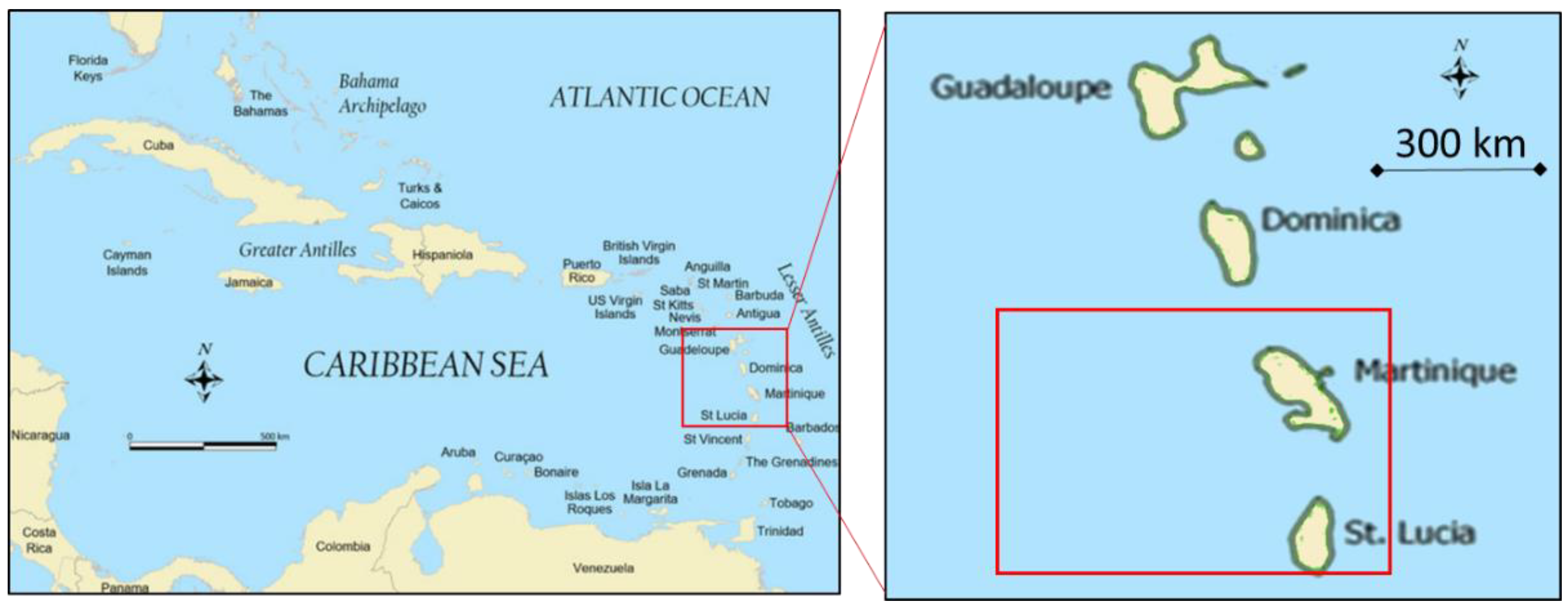
2.1. Study Area
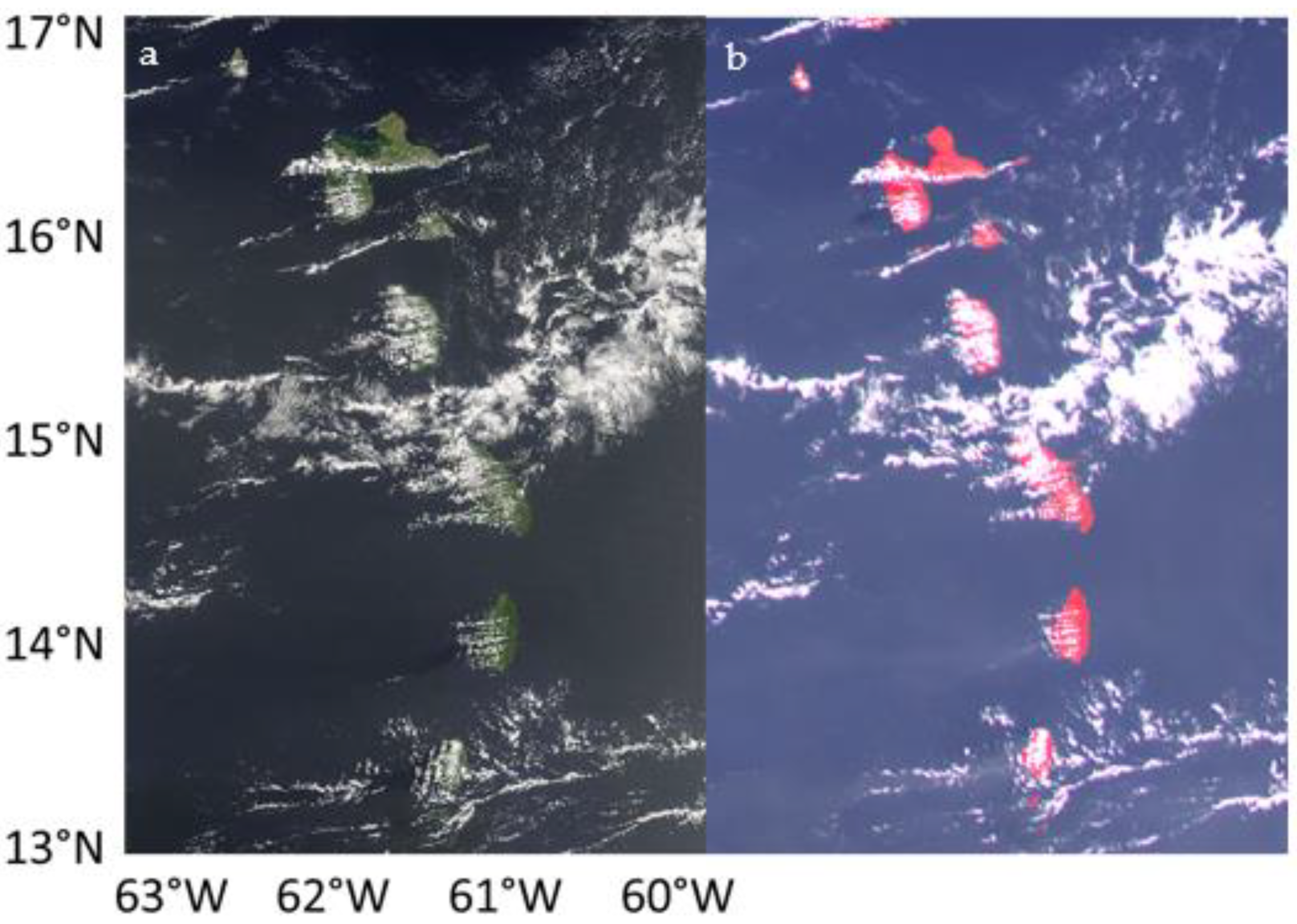
2.2. Satellite Data
2.3. Environmental Data
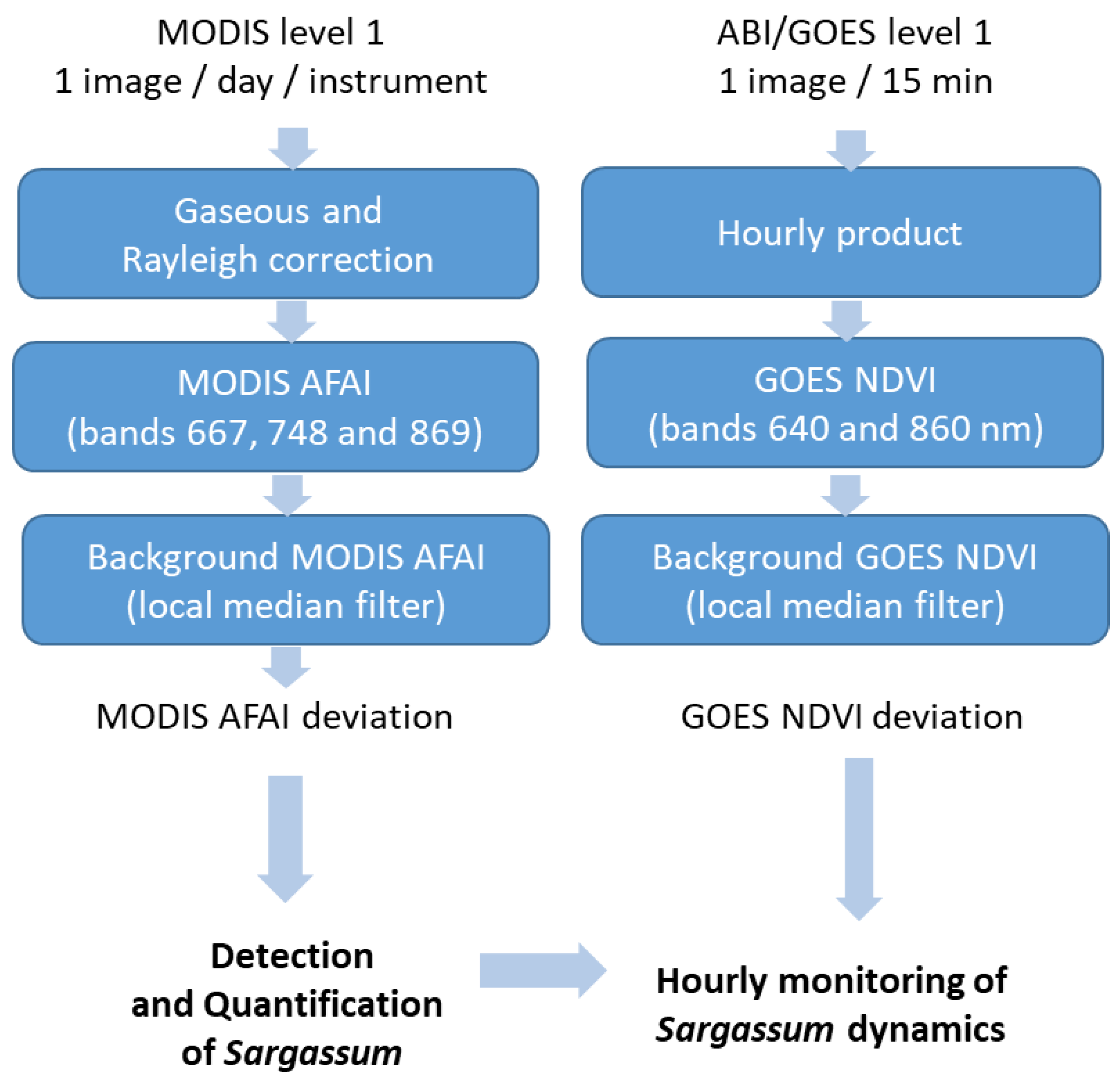
2.4. Methodology
3. Results
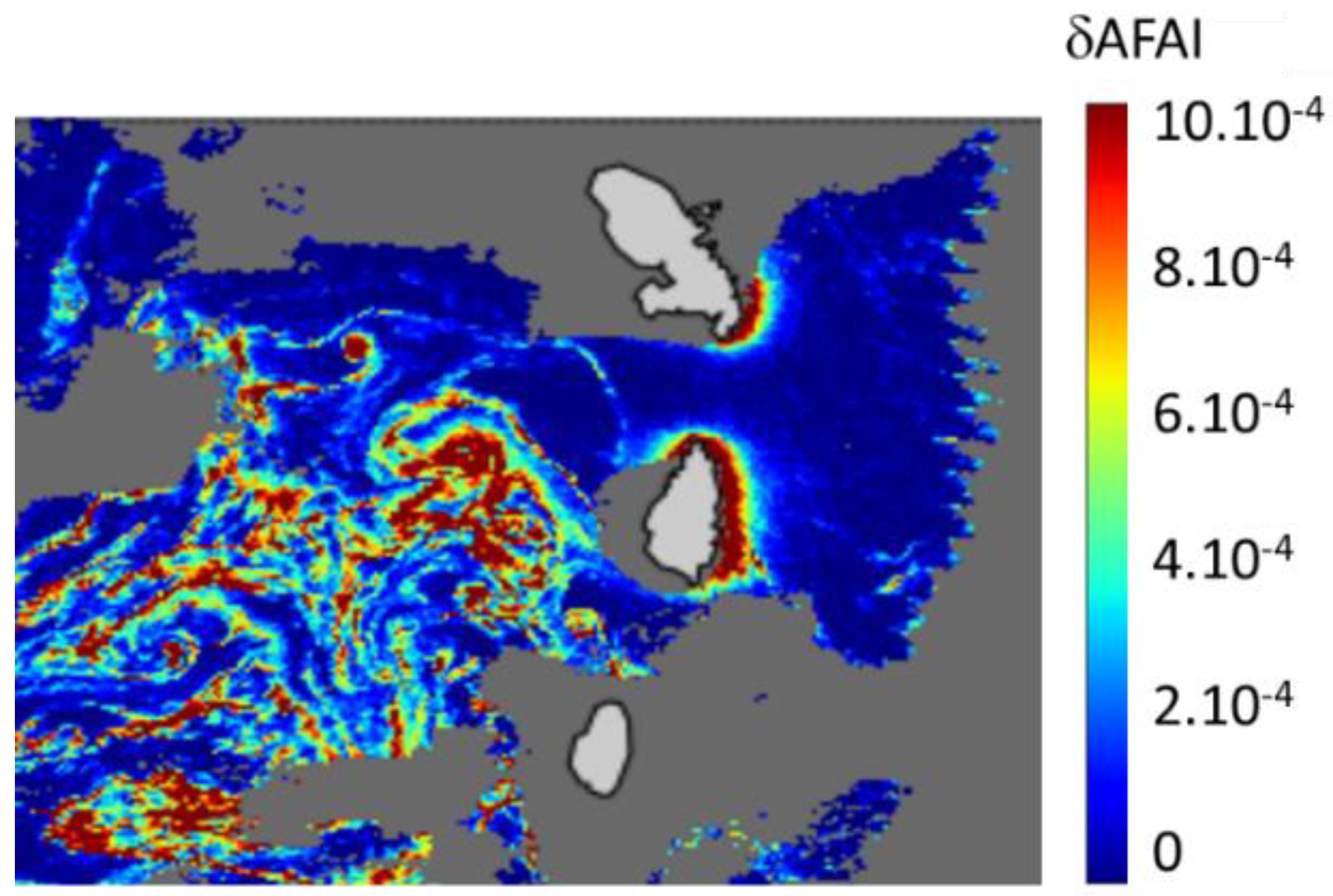
3.1. AFAI Deviation from MODIS
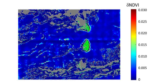
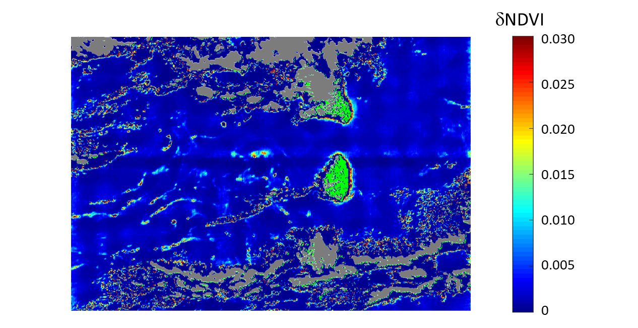
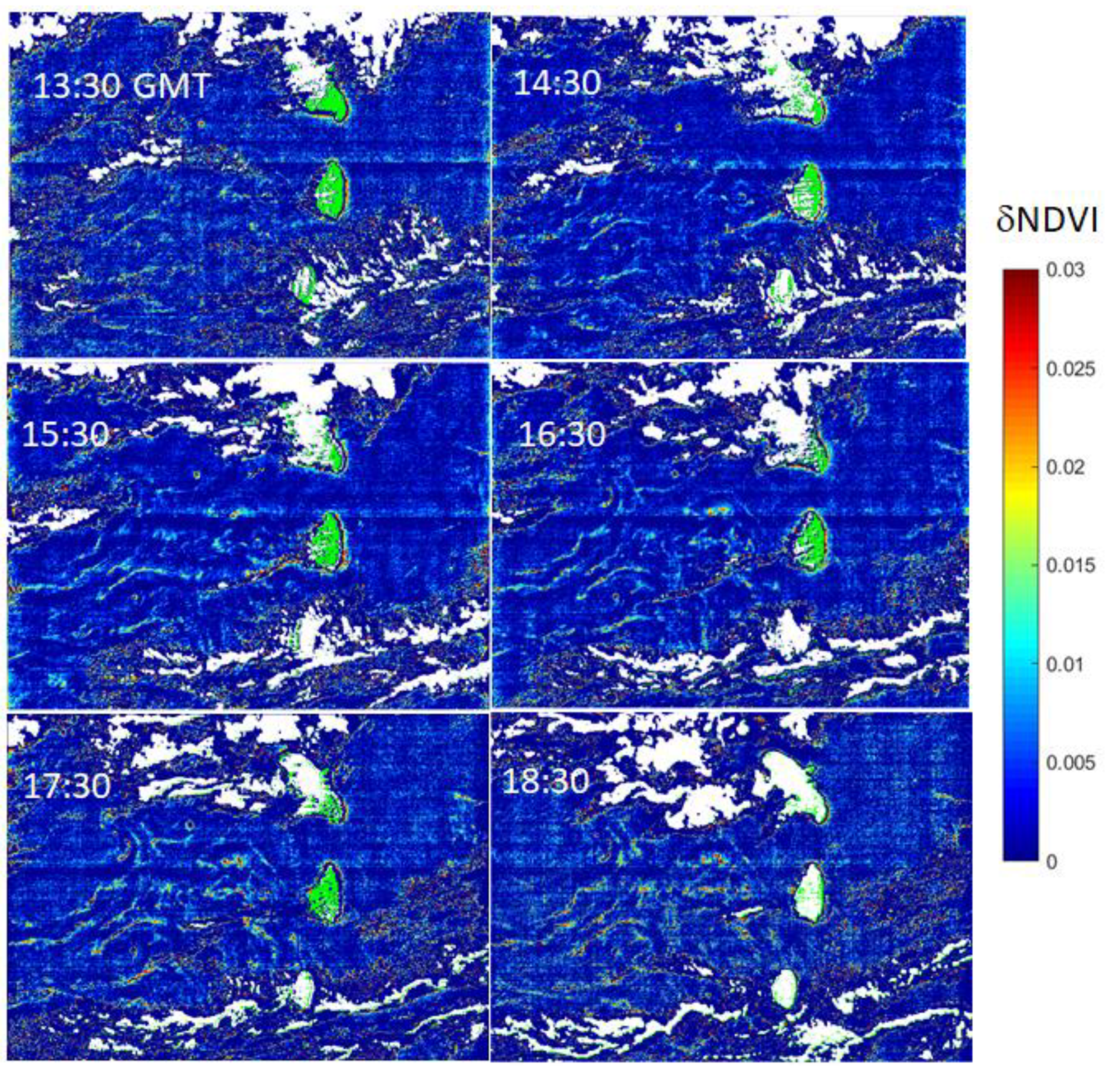
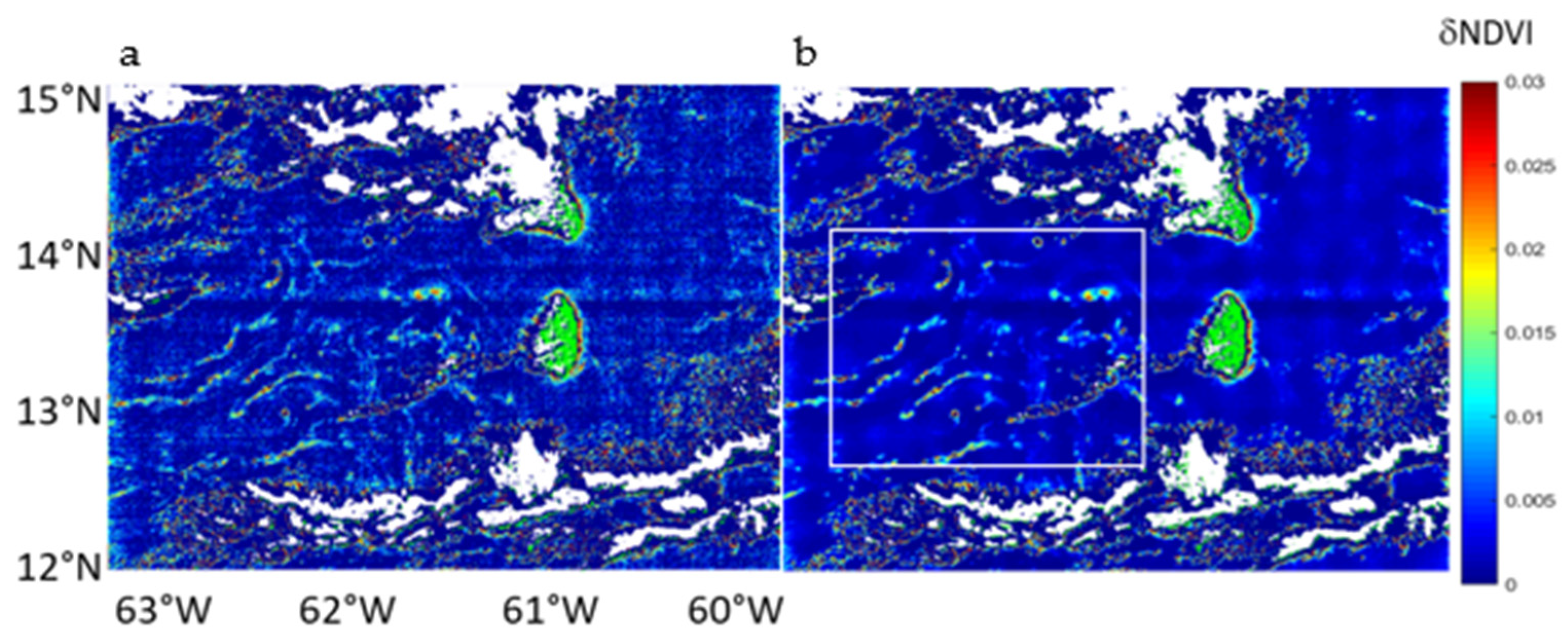
3.2. NDVI Deviation from GOES Hourly Product
3.3. GOES Noise Filtering
3.4. δNDVI Threshold Detection
3.5. Performance of GOES Algorithm for Sargassum Identification
4. Discussion
4.1. Impact of the Hourly GOES Product on the Noise Filtering and on the δNDVI Value
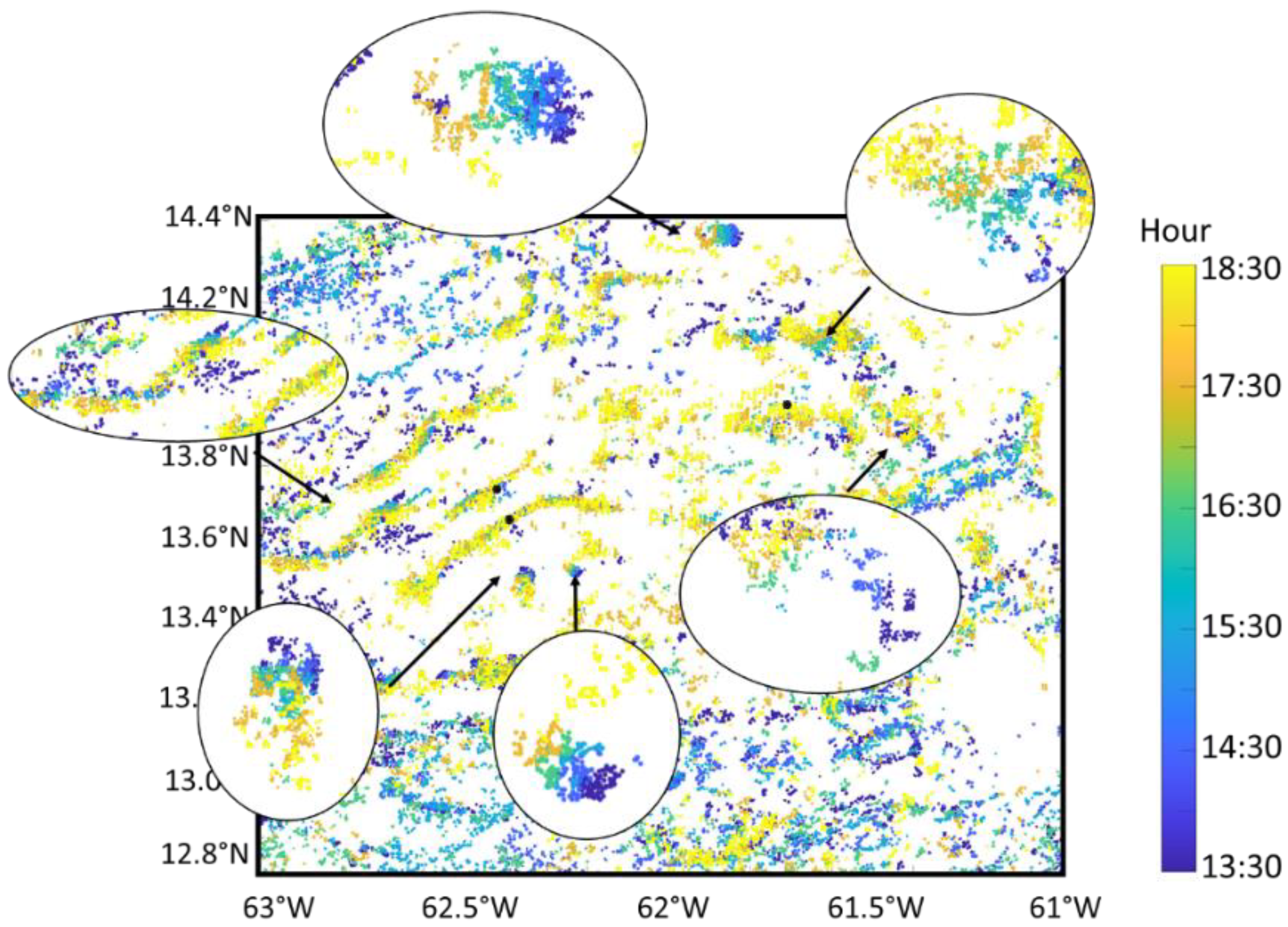
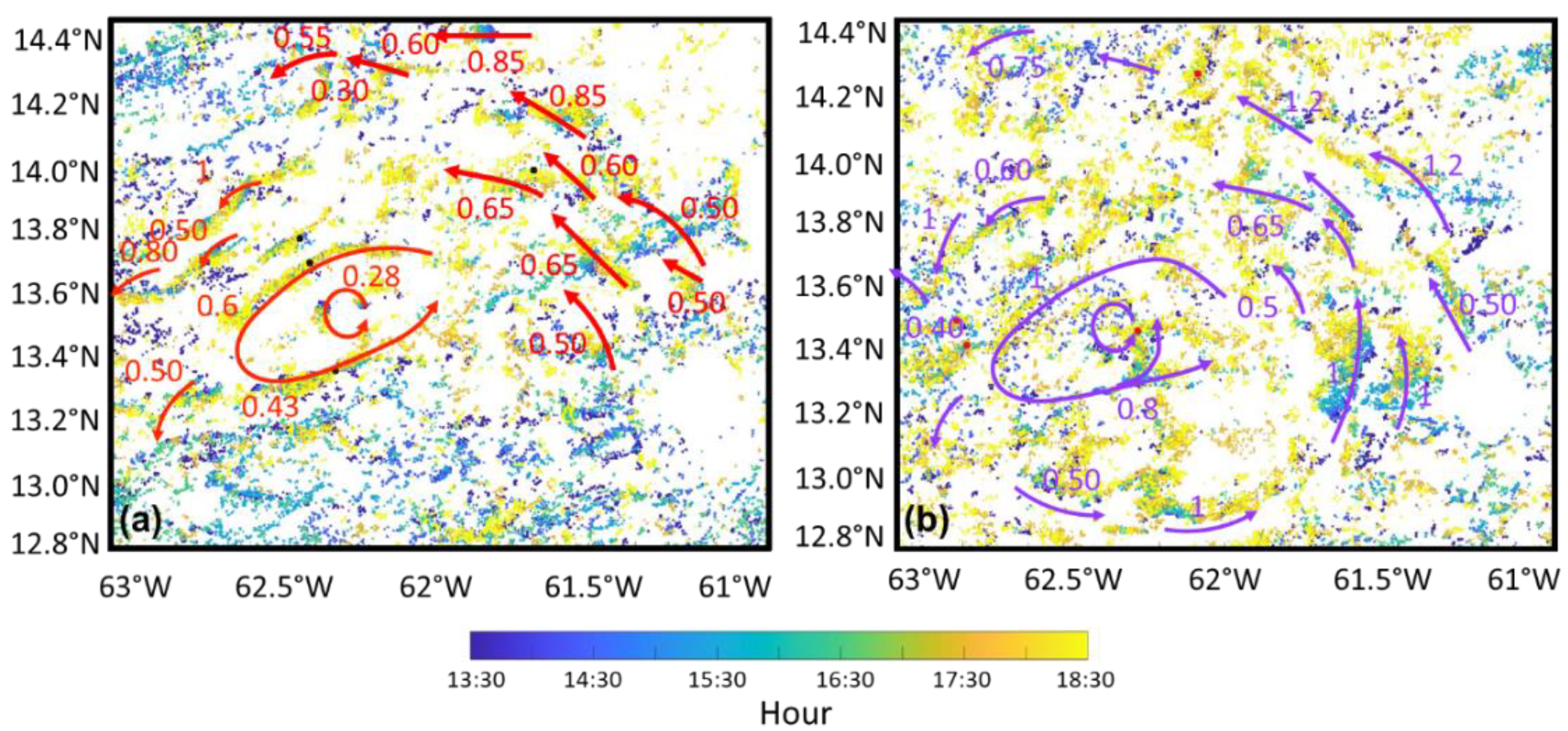
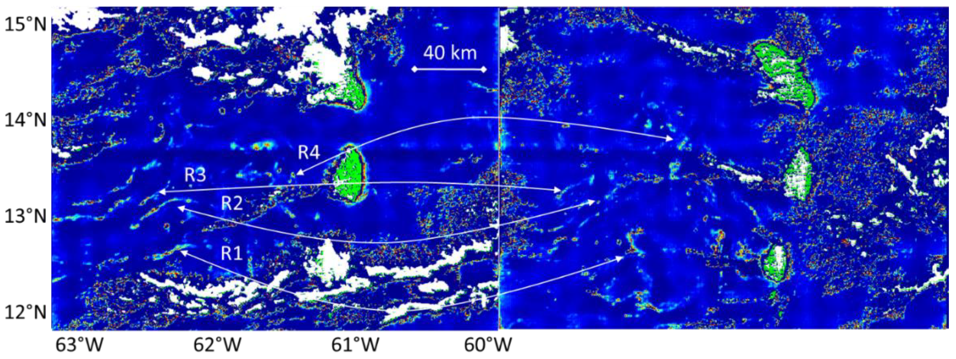
4.2. Sargassum Aggregation Tracking
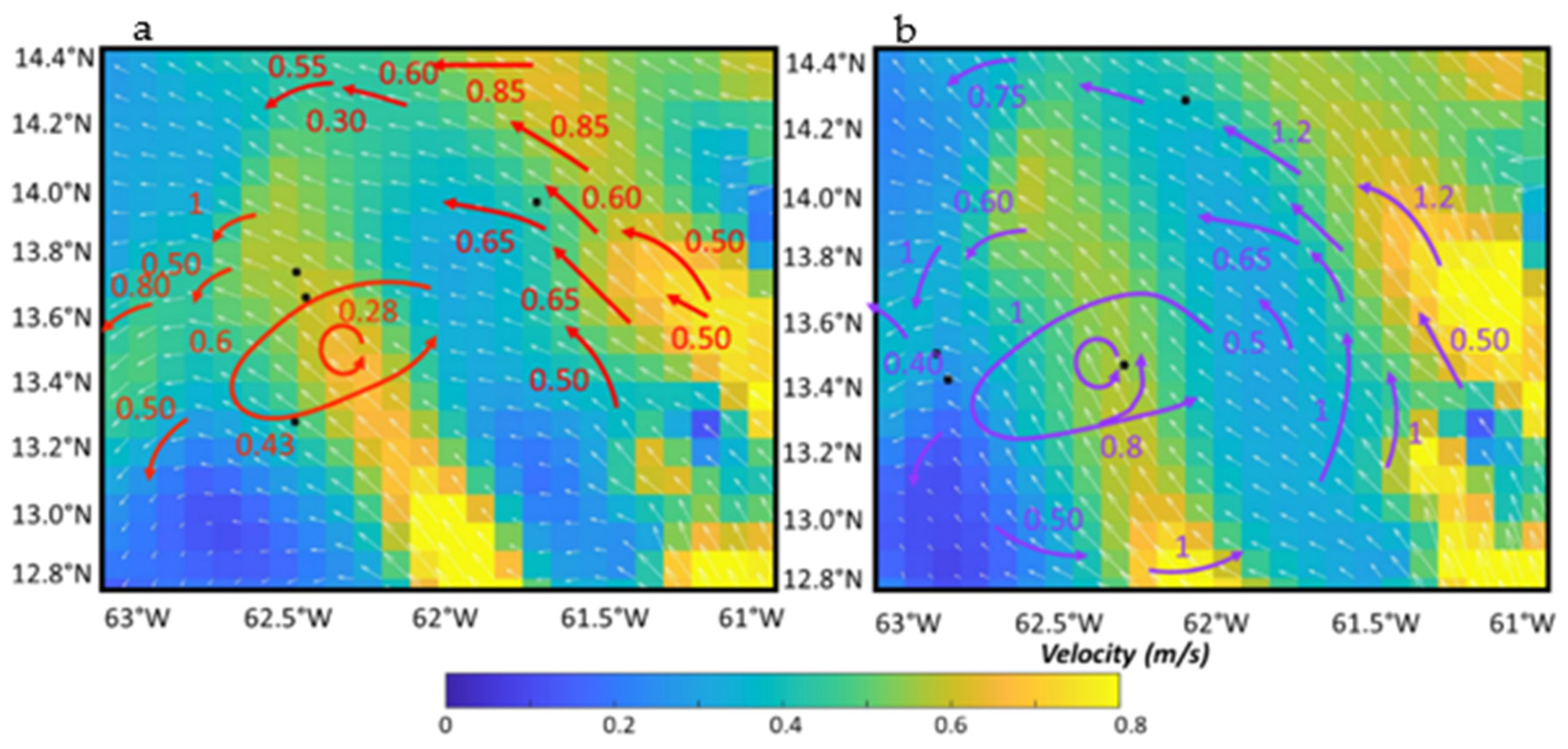
4.3. Consistency of Observed Drift with Satellite Derived Current and Temperature Data
4.4. Pertinence of GOES Sargassum Product for Transport Models
5. Conclusions
Supplementary Materials
Author Contributions
Funding
Acknowledgments
Conflicts of Interest
References
- Gower, J.; Hu, C.; Borstad, G.; King, S. Ocean Color Satellites Show Extensive Lines of Floating Sargassum in the Gulf of Mexico. IEEE Trans. Geosci. Remote. Sens. 2006, 44, 3619–3625. [Google Scholar] [CrossRef]
- Gower, J.; King, S.; Goncalves, P. Global monitoring of plankton blooms using MERIS MCI. Int. J. Remote. Sens. 2008, 29, 6209–6216. [Google Scholar] [CrossRef]
- Gower, J.F.; King, S.A. Distribution of floating Sargassum in the Gulf of Mexico and the Atlantic Ocean mapped using MERIS. Int. J. Remote Sens. 2011, 32, 1917–1929. [Google Scholar] [CrossRef]
- Gower, J.; Young, E.; King, S. Satellite images suggest a new Sargassum source region in 2011. Remote Sens. Lett. 2013, 4, 764–773. [Google Scholar] [CrossRef]
- Gower, J.; King, S. The distribution of pelagic Sargassum observed with OLCI. Int. J. Remote Sens. 2019, 41, 1–11. [Google Scholar] [CrossRef]
- Hu, C. A novel ocean color index to detect floating algae in the global oceans. Remote. Sens. Environ. 2009, 113, 2118–2129. [Google Scholar] [CrossRef]
- He, M.X.; Liu, J.; Yu, F.; Li, D.; Hu, C. Monitoring green tides in Chinese marginal seas. In Handbook of Satellite Remote Sensing Image Interpretation: Applications for Marine Living Resources Conservation and Management; Morales, J., Stuart, V., Platt, T., Sathyendranath, S., Eds.; EU PRESPO and IOCCG: Dartmouth, NS, Canada, 2011; pp. 111–124. [Google Scholar]
- Hu, C.; Li, D.; Chen, C.; Ge, J.; Muller-Karger, F.E.; Liu, J.; Yu, F.; He, M.X. On the recurrent Ulva prolifera blooms in the Yellow Sea and East China Sea. J. Geophys. Res. Ocean. 2010, 115. [Google Scholar] [CrossRef]
- Hu, C.; Feng, L.; Hardy, R.F.; Hochberg, E.J. Spectral and spatial requirements of remote measurements of pelagic Sargassum macroalgae. Remote. Sens. Environ. 2015, 167, 229–246. [Google Scholar] [CrossRef]
- Wang, M.; Hu, C. Mapping and quantifying Sargassum distribution and coverage in the Central West Atlantic using MODIS observations. Remote Sens. Environ. 2016, 183, 350–367. [Google Scholar] [CrossRef]
- Ody, A.; Thibaut, T.; Berline, L.; Changeux, T.; André, J.-M.; Chevalier, C.; Blanfuné, A.; Blanchot, J.; Ruitton, S.; Stiger-Pouvreau, V.; et al. From In Situ to satellite observations of pelagic Sargassum distribution and aggregation in the Tropical North Atlantic Ocean. PLoS ONE 2019, 14, e0222584. [Google Scholar] [CrossRef]
- Wang, M.; Hu, C.; Cannizzaro, J.; English, D.; Han, X.; Naar, D.; Lapointe, B.; Brewton, R.; Hernandez, F. Remote Sensing of Sargassum Biomass, Nutrients, and Pigments. Geophys. Res. Lett. 2018, 45, 12–359. [Google Scholar] [CrossRef]
- Kwon, K.; Choi, B.-J.; Kim, K.Y.; Kim, K. Tracing the trajectory of pelagic Sargassum using satellite monitoring and Lagrangian transport simulations in the East China Sea and Yellow Sea. ALGAE 2019, 34, 315–326. [Google Scholar] [CrossRef]
- Rouse, J.W.; Haas, R.H.; Schell, J.A.; Deering, D.W. Monitoring vegetation systems in the Great Plains with ERTS. NASA Spec. Publ. 1974, 351, 309. [Google Scholar]
- Tucker, C.J. Red and photographic infrared linear combinations for monitoring vegetation. Remote. Sens. Environ. 1979, 8, 127–150. [Google Scholar] [CrossRef]
- van Tussenbroek, B.I.; Arana, H.A.; Rodríguez-Martínez, R.E.; Espinoza-Avalos, J.; Canizales-Flores, H.M.; González-Godoy, C.E.; Barba-Santos, M.G.; Vega-Zepeda, A.; Collado-Vides, L. Severe impacts of brown tides caused by Sargassum spp. on near-shore Caribbean seagrass communities. Mar. Pollut. Bull. 2017, 122, 272–281. [Google Scholar] [CrossRef]
- Resiere, D.; Mehdaoui, H.; Florentin, J.; Gueye, P.; Lebrun, T.; Blateau, A.; Viguier, J.; Valentino, R.; Brouste, Y.; Kallel, H.; et al. Sargassum seaweed health menace in the Caribbean: Clinical characteristics of a population exposed to hydrogen sulfide during the 2018 massive stranding. Clin. Toxicol. 2021, 59, 215–223. [Google Scholar] [CrossRef] [PubMed]
- Berline, L.; Ody, A.; Jouanno, J.; Chevalier, C.; André, J.-M.; Thibaut, T.; Ménard, F. Hindcasting the 2017 dispersal of Sargassum algae in the Tropical North Atlantic. Mar. Pollut. Bull. 2020, 158, 111431. [Google Scholar] [CrossRef] [PubMed]
- Savtchenko, A. Terra and Aqua MODIS products available from NASA GES DAAC. Adv. Space Res. 2004, 34, 710–714. [Google Scholar] [CrossRef]
- Kalluri, S.; Alcala, C.; Carr, J.; Griffith, P.; Lebair, W.; Lindsey, D.; Race, R.; Wu, X.; Zierk, S. From Photons to Pixels: Processing Data from the Advanced Baseline Imager. Remote. Sens. 2018, 10, 177. [Google Scholar] [CrossRef]
- Aminou, D.M.A.; Ottenbacher, A.; Hanson, C.G.; Pili, P.; Müller, J.; Blancke, B.; Jacquet, B.; Bianchi, S.; Coste, P.; Pasternak, F.; et al. Meteosat Second Generation: The MSG-1 imaging radiometer performance results at the end of the commissioning phase. In Proceedings of the Earth Observing Systems VIII; Optical Science and Technology, SPIE’s 48th Annual Meeting, San Diego, CA, USA, 10 November 2003; Volume 5151, pp. 599–608. [Google Scholar]
- Bonjean, F.; Lagerloef, G.S. Diagnostic model and analysis of the surface currents in the tropical Pacific Ocean. J. Phys. Oceanogr. 2002, 32, 2938–2954. [Google Scholar] [CrossRef]
- Jouanno, J.; Benshila, R.; Berline, L.; Soulié, A.; Radenac, M.H.; Morvan, G.; Diaz, F.; Sheinbaum, J.; Chevalier, C.; Thibaut, T.; et al. A NEMO-based model of Sargassum distribution in the Tropical Atlantic: Description of the model and sensitivity analysis (NEMO-Sarg1. 0). Geosci. Model Dev. Discuss 2020, 1–30. [Google Scholar] [CrossRef]
- Von Schuckmann, K.; Le Traon, P.-Y.; Alvarez-Fanjul, E.; Axell, L.; Balmaseda, M.; Breivik, L.-A.; Brewin, R.J.W.; Bricaud, C.; Drevillon, M.; Drillet, Y.; et al. The Copernicus Marine Environment Monitoring Service Ocean State Report. J. Oper. Oceanogr. 2016, 9, s235–s320. [Google Scholar] [CrossRef]
- Siegel, D.A.; Wang, M.; Maritorena, S.; Robinson, W. Atmospheric correction of satellite ocean color imagery: The black pixel assumption. Appl. Opt. 2000, 39, 3582–3591. [Google Scholar] [CrossRef]
- Parker, J.A.; Kenyon, R.V.; Troxel, D.E. Comparison of Interpolating Methods for Image Resampling. IEEE Trans. Med Imaging 1983, 2, 31–39. [Google Scholar] [CrossRef]
- Buades, A.; Coll, B.; Morel, J.-M. A review of image denoising algorithms, with a new one. SIAM Multiscale Modeling Simul. 2005, 4, 490–530. [Google Scholar] [CrossRef]
- Buades, A.; Coll, B. Non-local means denoising. Image Process. Line 2011, 1, 208–212. [Google Scholar] [CrossRef]


| Drift Velocity m·s−1 | Drift Distance | Drift Velocity m·s−1 | |||
|---|---|---|---|---|---|
| 8 August— t = 5 h | 9 August— t = 5 h | t = 19 h (from 18:30 on 8 August to 13:30 on 9 August) | Averaged Over the 2 Days | Direction | |
| Aggregation 1 (R1) | 0.4 | 0.8 | 41 km | 0.6 | along the eddy |
| Aggregation 2 (R2) | 0.6 | 1 | 55 km | 0.80 | along the eddy |
| Aggregation 3 (R3) | 0.5 | 1 | 51 km | 0.75 | along the eddy |
| Aggregation 4 (R4) | 0.5 | 1.2 | 58 km | 0.85 | northwestward |
Publisher’s Note: MDPI stays neutral with regard to jurisdictional claims in published maps and institutional affiliations. |
© 2021 by the authors. Licensee MDPI, Basel, Switzerland. This article is an open access article distributed under the terms and conditions of the Creative Commons Attribution (CC BY) license (https://creativecommons.org/licenses/by/4.0/).
Share and Cite
Minghelli, A.; Chevalier, C.; Descloitres, J.; Berline, L.; Blanc, P.; Chami, M. Synergy between Low Earth Orbit (LEO)—MODIS and Geostationary Earth Orbit (GEO)—GOES Sensors for Sargassum Monitoring in the Atlantic Ocean. Remote Sens. 2021, 13, 1444. https://doi.org/10.3390/rs13081444
Minghelli A, Chevalier C, Descloitres J, Berline L, Blanc P, Chami M. Synergy between Low Earth Orbit (LEO)—MODIS and Geostationary Earth Orbit (GEO)—GOES Sensors for Sargassum Monitoring in the Atlantic Ocean. Remote Sensing. 2021; 13(8):1444. https://doi.org/10.3390/rs13081444
Chicago/Turabian StyleMinghelli, Audrey, Cristele Chevalier, Jacques Descloitres, Léo Berline, Philippe Blanc, and Malik Chami. 2021. "Synergy between Low Earth Orbit (LEO)—MODIS and Geostationary Earth Orbit (GEO)—GOES Sensors for Sargassum Monitoring in the Atlantic Ocean" Remote Sensing 13, no. 8: 1444. https://doi.org/10.3390/rs13081444
APA StyleMinghelli, A., Chevalier, C., Descloitres, J., Berline, L., Blanc, P., & Chami, M. (2021). Synergy between Low Earth Orbit (LEO)—MODIS and Geostationary Earth Orbit (GEO)—GOES Sensors for Sargassum Monitoring in the Atlantic Ocean. Remote Sensing, 13(8), 1444. https://doi.org/10.3390/rs13081444