Article

Wetlands Cool Land Surface Temperature in Tropical Regions but Warm in Boreal Regions

Sino-French Institute for Earth System Science, College of Urban and Environmental Sciences, Peking University, Beijing 100871, China
*
Author to whom correspondence should be addressed.
Remote Sens. 2021, 13(8), 1439; https://doi.org/10.3390/rs13081439
Submission received: 17 February 2021 / Revised: 26 March 2021 / Accepted: 5 April 2021 / Published: 8 April 2021
(This article belongs to the Section Environmental Remote Sensing)

Abstract

:
Wetlands play a critical role in global hydrological and biogeochemical cycles. Regulating the regional climate is one of the most important ecosystem services of natural wetlands. However, the impact of wetlands on local temperature on the global scale and the attribution is still unclear. This study utilizes the satellite-based products (land surface temperature (LST), albedo, and evapotranspiration (ET)) to evaluate the difference in LST between wetlands and their adjacent landcover types and the possible drivers. Here we show that on average for the whole year, wetlands have a cooling effect in tropical regions, but have a warming effect in boreal regions. The impacts of wetlands on LST show great seasonality in the boreal regions; i.e., the wetlands have a warming effect in winter but a cooling effect in summer. The difference in albedo and ET between wetlands and the other landcover types only interprets 30% of temporal variation of the difference in LST. Due to the large water storage in wetlands, the ground heat flux (G) may interpret the rest of the impact, absorbing energy in summer and releasing energy in winter in wetlands, which has often been neglected in previous studies. Our results indicate that it is critical to comprehensively consider the effects of wetland restoration in different regions to realize potential climatic benefits in the future.

Graphical Abstract

1. Introduction

Wetlands cover only 10% (13.0 million km2) of the world’s land surface area [1], but exert critical impacts on global hydrological and biogeochemical cycles, as well as biodiversity conservation [2,3,4,5]. Due to climate change and the intensifying human activities, however, both satellite images and wetland inventories suggest a decline in the area of natural wetlands around the world [6,7,8]. For instance, the Global Wetland Outlook 2018 reported an approximately 35% decrease of inland and marine/coastal wetlands between 1970 and 2015 [4]. In turn, some essential ecosystem services of natural wetlands such as water purification, flood control, and climate regulation could be jeopardized. As the threat of climate change has grown more severe, the feedbacks between climate and wetlands could be intensified and cause unexpected consequences. Therefore, identifying and understanding the ecosystem services of natural wetlands is critical to sustainable development goals [9].
Regulating the regional climate is one of the most important ecosystem services of natural wetlands [10]. According to the radiation budget equation on an ecosystem scale, the net radiation, Rnet, i.e., the balance between the inputs and outputs of shortwave (Kin and Kout) and longwave radiation (Lin and Lout ), is approximately balanced by the energy that is transferred out of the ecosystem by non-radiative processes including sensible heat flux (H), latent heat flux (LE), ground heat flux (G), and the change in chemical energy stored in the ecosystem (ΔS) [11]:
Rnet = Kin − Kout + Lin − Lout = H + LE + G + ΔS
With dark water surface and dense vegetation, wetlands tend to have a lower albedo and thus receive more net radiation in contrast to adjacent drylands (the incoming solar radiation is expected to be very comparable for all grids due to proximity) [12]. On the other hand, the existence of vegetation and water surface in wetland grids could result in significant differences in the transformation of available energy into latent and sensible heat fluxes (i.e., LE and H, respectively) as well as surface roughness against ambient other landscapes. If the ground heat flux G is always negligible, the wetland will have a cooler surface if more net radiation is dissipated as LE, compared with other landscapes (ΔS is only <5% of net shortwave radiation [13]); otherwise, the wetland will have a warmer surface. Most station-based studies suggested a surface cooling effect for wetlands, probably due to the increased latent heat when comparing the surface temperature in wetlands and other adjacent landscapes [14,15]. For example, Bai et al. [16] indicated that soil temperature is higher in an area surrounded with less wetland. Zheng et al. [17] found that the land surface temperature (LST) in the Minjiang River estuary increased during the wetland deterioration period (1993–2013), indicating a cooling effect of wetlands without deterioration [17]. Given that, in summer and autumn, more heat could be moved away from the wetland surface due to the large heat capacity of the water body and turbulent mixing capability of water/vapor fluxes, the ground heat flux G in wetlands is substantial and plays an important role on LST in these two seasons. Yet the ground heat flux G has been neglected in most existing studies about the impacts of land-use change on LST [18,19], and also in the evaluation of the impacts of wetlands on local/regional climate. Moreover, the attribution of the climatic impacts of wetlands on the global scale is still scarce and needs to be investigated.
In this study, we use a satellite-derived LST product during the period 2001–2017 to verify the impacts of wetlands on climate. The differences of albedo and evapotranspiration (ET) between wetlands and adjacent other landscapes (including forest, shrubland, and open land) are adopted to investigate the radiative and nonradiative impacts of wetlands, respectively. The primary objectives of this investigation are to (1) characterize the annual and seasonal climatic impacts of global natural wetlands, and (2) interpret the net climatic impacts of wetlands from the radiative (i.e., albedo) and nonradiative (i.e., H, LE, and G) biophysical aspects.

2. Materials and Methods

2.1. Data

In this study, the LST products and landcover maps derived from MODIS (Moderate Resolution Imaging Spectroradiometer) with a spatial resolution of 1 × 1 km were utilized to investigate the annual and seasonal climatic impacts of global natural wetlands. Specifically, the difference in LST between wetland pixels and other landcover types (ΔLST) was estimated for each 0.5 × 0.5° grid cell. Following that, the albedo and ET data from MODIS were analyzed to interpret the ΔLST between wetland pixels and other landscapes, from radiative and nonradiative aspects, respectively. More details for these data and relevant analyses are provided below.

2.1.1. Land Use and Landcover Data

The MODIS land use and landcover map (MCD12Q1) in 2001, with an overall accuracy of 75% from the cross-validation accuracy assessment [20], were used to distinguish wetland, forest, shrubland, and open land pixels. This dataset encompasses 17 landcover classes proposed by the International Geosphere–Biosphere Program (IGBP), of which class 11, class 1–5, class 6–9, and class 10, 12, 14 represent permanent wetlands, forest, and open lands, respectively. Open lands include cropland, grassland, or a mix of cropland and grassland. The absolute area and the fraction of the land surface area of the 17 classes are summarized by the statistics in Table 1. According to the IGBP classification, only permanently inundated lands with 30–60% water cover and >10% vegetated cover were identified as wetlands, such that in the following analysis global natural wetlands covered only 0.73% (1.1 million km2) of the land surface area (see Table 1), which is much less than those in other studies where the seasonally inundated wetlands are included [1]. Note that the area of permanent wetlands in 2001 was the lowest during the period 2001–2017. We used the landcover map of 2001 as the minimum area of wetlands. We also tested that our results were robust with landcover maps of other years.

2.1.2. LST Data

The LST is the radiative skin temperature of the land surface, as measured in the direction of the remote sensor, and LST is a mixture of vegetation and bare soil temperatures [21]. The LST data were obtained from the MODIS Earth Observing System Terra instruments, which are sun-synchronous and image the entire Earth every 1–2 days. Thus, a daytime (local solar time ~10:30 a.m. from Terra) and a nighttime (~10:30 p.m. from Terra) temperature observation at a 1 × 1 km resolution could be provided every 8 days. This product has been widely used at more than 42 sites in Greenland, China, Europe, and Africa and is proven to be of high quality [22], with errors less than 1 °C [23]. In our analysis, the daytime and nighttime LST were averaged to obtain the daily mean values during the period 2001–2017.

2.1.3. Albedo Data

The MODIS black-sky albedo (or directional hemispherical reflectance) (MCD43D51), a concept of albedo in the absence of a diffuse component with shortwave broadband (0.3–5.0 μm) of solar radiation, was utilized because it can describe the energy difference between different landcover types. In MODIS, black sky albedo products are available from 2001 to 2017 with a spatial resolution of 30 s (1 km) and a time resolution of 8-day intervals. The uncertainty of albedo data is up to 0.02 (10%) [24], and has been extensively validated in typical landcover types [25].

2.1.4. ET Data

The MODIS ET data (MOD16A2), 8-day composite data available from 2001 to 2017, is utilized here because it has a spatial resolution of 500 m, which is much finer compared to other ET products. The data was derived from the daily meteorological reanalysis products and 8-day remotely sensed dynamics of vegetation characteristics; thus, it was independent of the MODIS LST product. The mean absolute errors between ET estimates in this dataset and observations from ground-based flux measurements are 0.33 kg m−3 day−1 [26]. It should be noted that the MOD16 evaporation algorithm has the best performance for forests while it has mismatches for grasslands [27].

2.1.5. Air Temperature, Radiation, and Elevation Data

The CERES–EBAF shortwave fluxes at 1° resolution in the all-sky scene from the Clouds and the Earth’s Radiant Energy System (CERES) project website (https://ceres.larc.nasa.gov/data/, accessed on 10 May 2019) were used to calculate energy from solar shortwave radiation. We also used the monthly air temperature (Tair) data during the period 2001–2017 from the Climate Research Unit (CRU) time-series v4.02 climate data [28] to compare with the LST with a spatial resolution of 0.5 × 0.5°. Furthermore, to minimize the impact of elevation on ΔLST, the SRTM (Shuttle Radar Topography Mission) elevation data at 1 arc-second (30 m) resolution were used to remove grid cells with elevation difference between wetlands, forests, shrublands, and open lands larger than 100 m.

2.2. Methods

All datasets are in the WGS84 geographic coordinate system. First, we split the world into regular 0.5 × 0.5° grid cells. In each grid cell, we calculated the mean LST, albedo and ET of all 1 km or 500 m pixels of each landcover type. Then, the ΔLST, Δalbedo and ΔET between wetlands and other adjacent landcover types were derived for each 0.5 × 0.5° grid. The land covers in the same 0.5 × 0.5° grid cell were regarded as adjacent landscapes. We defined the 0.5 × 0.5° grid cells with wetland fraction larger than 1% in the land use and landcover map as “wetlands” grids, and grids with a wetland fraction smaller than 1% were masked out. Then we removed grid cells with elevation difference between wetlands, forests, shrublands, and open lands larger than 100 m. Finally, only 2335, 2336, and 1599 sample grids were obtained for the comparison of ΔLST between wetlands and forests, shrublands, and open lands, respectively. Globally, permanent wetlands are mainly located in northwest Canada, West Siberia, Amazon, Congo Basin, and the Malay Archipelago (Figure 1). The global mean annual air temperature, LST, and albedo of these permanent wetlands are 9.7 ± 14.4 °C, 7.8 ± 14.6 °C, and 0.2 ± 0.1, respectively (Figures S1 and S2). Wetlands in different regions may have different spatial patterns of ΔLST, which can be governed by different underlying mechanisms. The typical regions were selected to characterize a class/type of underlying mechanisms for corresponding spatial patterns of ΔLST (Figure 1).
Comparing the difference in surface energy fluxes between wetlands and other adjacent landcover types, Equation (1) can be reformulated as follows:
ΔRnet =ΔK +ΔL =ΔH + ΔLE +ΔG + ΔS’
where ΔK and ΔL are the differences of shortwave and longwave radiation, respectively; ΔRnet is the difference in net radiation; ΔH, ΔLE, and ΔG are the differences in sensible, latent, and ground heat flux respectively; and ΔS’ is the difference in the change of chemical energy storage. In the calculation of the difference in surface energy fluxes between wetlands and the other adjacent landcover types, ΔK (the difference of shortwave radiation) was calculated by multiplying Δalbedo and the energy flux of solar shortwave radiation, and ΔLE (the difference of latent heat flux) was calculated by multiplying ΔET and latent heat of vaporization at 2.45 MJ/kg. The sum of effects of Δalbedo and ΔET is noted as ΔSEF, equal to the sum of ΔK and ΔLE, which are two major energy fluxes that impact ΔLST. For the effects of other energy fluxes (ΔL, ΔH, ΔG, and ΔS’) on ΔLST, we discussed these effects in Section 4.2. To attribute the effect of Δalbedo and ΔLE to the temporal variation of ΔLST, we performed a dominance analysis based on the multiple linear regression model [29]. The dominance analysis has been widely used for quantifying the relative importance of predictors based on the decomposition of R2 [30]. In our study, the dominance analysis was conducted with the “relaimpo” package in R to derive the relative importance of Δalbedo and ΔET for the temporal variation of monthly ΔLST.

3. Results

3.1. Spatial Patterns of Mean Annual ΔLST

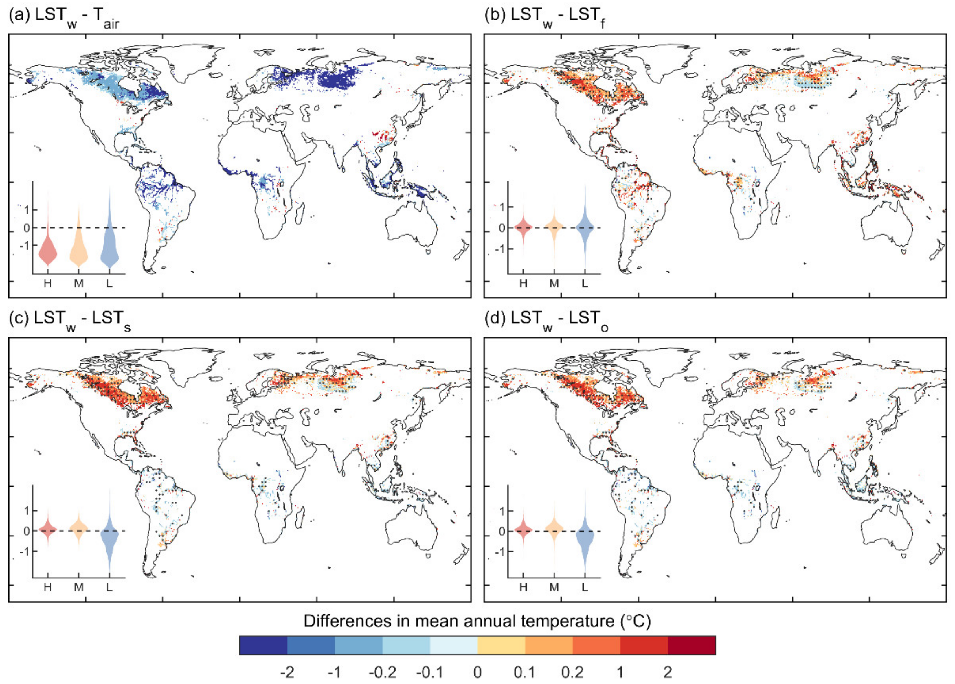
Figure 2 illustrates the spatial patterns of mean annual ΔLST between wetlands and three ambient landcover types, denoted by Δ LST f w , Δ LST s w , and Δ LST o w , respectively. As shown in Figure 2, although the global mean values of Δ LST f w , Δ LST s w , and Δ LST o w were relatively small (0.0 ± 0.6, −0.1 ± 0.6, and −0.1 ± 0.7 °C, respectively) compared to the difference between LST and air temperature in wetlands ( Δ LST a w , −2.1 ± 1.3 °C), regional and latitudinal differences were found in the Δ LST f w , Δ LST s w , and Δ LST o w . In boreal regions (>60°N, Northeast Canada and West Siberia), more than 55% of the regions (except the south part of West Siberia) had positive ΔLST (with mean values of 0.0 ± 0.2, 0.1 ± 0.2, and 0.1 ± 0.2 °C for Δ LST f w , Δ LST s w , and Δ LST o w , respectively), indicating that the LST of wetlands was higher than those in forests, shrublands, and open lands. In tropical regions (30°S–30°N, Amazon, Congo Basin, and the Malay Archipelago), more than 70% of the region (most in the Amazon Basin and Malaysia) had negative ΔLST (−0.3 ± 0.9 °C), indicating that the LST of wetlands was lower than those in the three other landcover types. Therefore, the general spatial/latitudinal patterns of ΔLST indicated a warming effect of natural wetlands in boreal regions but a cooling effect in the low-latitude tropical regions.

3.2. Spatial Patterns of Seasonal ΔLST

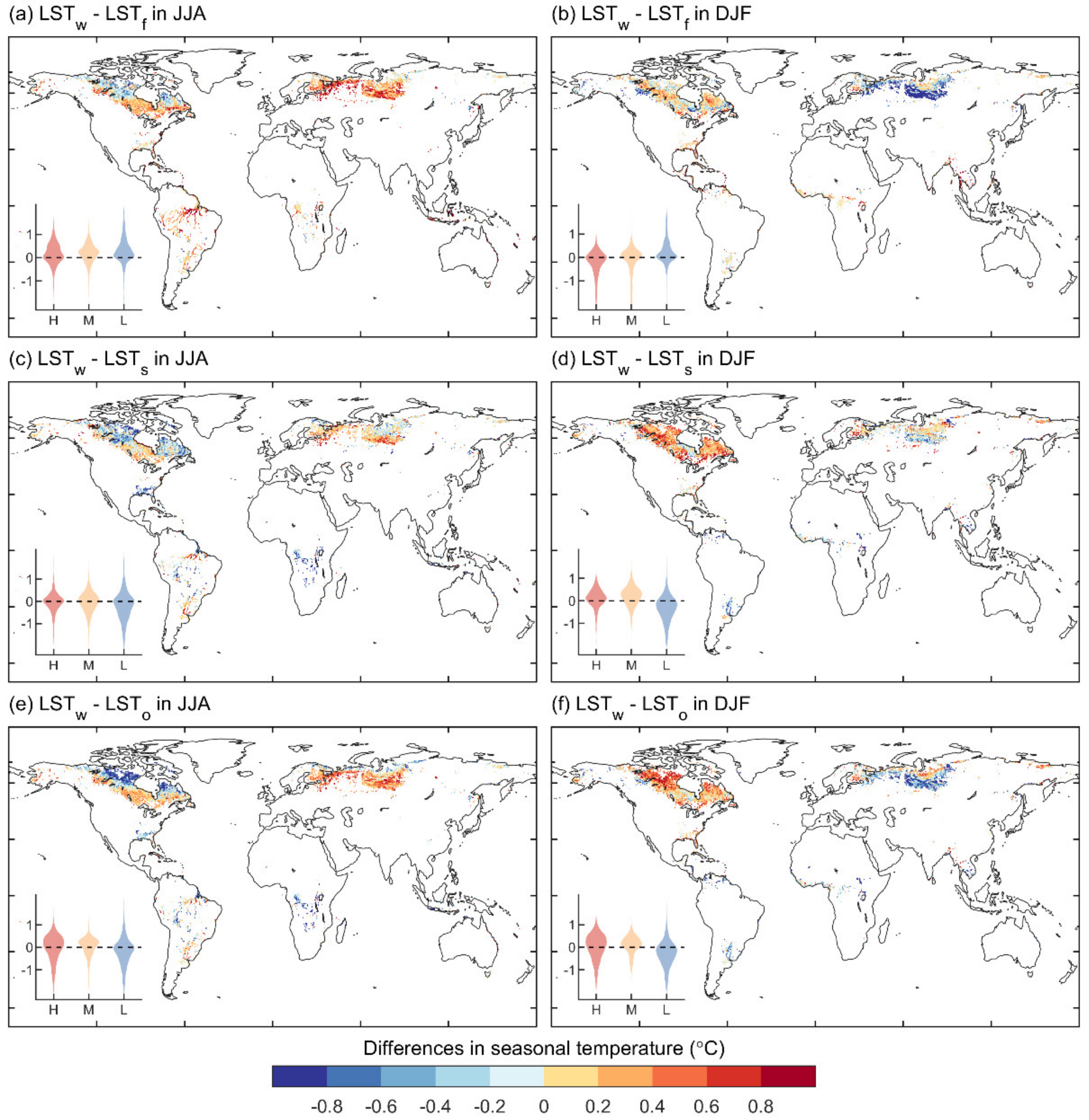
The spatial patterns of ΔLST (i.e., Δ LST f w , Δ LST s w , and Δ LST o w ) were found to have significant differences as the seasons shifted. Because of the similarity embedded in spatial patterns in spring (March–May [MAM]) and summer (June–August [JJA]) as well as those in autumn (September–November [SON]) and winter (December–February [DJF]), Figure 3 compares the spatial patterns of ΔLST in summer and winter. The comparison of those in MAM and SON is shown in Figure S3 and the statistics of ΔLST in four typical regions is shown in Table S1. In tropical regions, about 70% of wetland grids had negative Δ LST s w , and Δ LST o w (i.e., −0.2 ± 0.6 and −0.1 ± 0.6 °C) but positive Δ LST f w (0.3 ± 0.6 °C) across all seasons. In summer, most of the wetlands in the boreal latitude regions had negative ΔLST, indicating that the LST in wetlands was lower than those in the other three landcover types; i.e., wetlands had a cooling effect. In winter, about 70% of wetlands in the high-latitude regions (mostly in Canada) had positive Δ LST s w (0.2 ± 0.5 °C) and Δ LST o w (0.1 ± 0.5 °C) but negative Δ LST f w (−0.2 ± 0.7 °C), indicating that LST in wetlands was higher than those in shrublands and open lands but lower than those in forests; i.e., wetlands had a warming effect over shrublands and open lands but a cooling effect over forests. The winter (and autumn) ΔLST between wetlands and other landcover types in the boreal region dominated the signal of mean annual ΔLST.

3.3. Spatial Patterns of Seasonal Δalbedo and ΔET

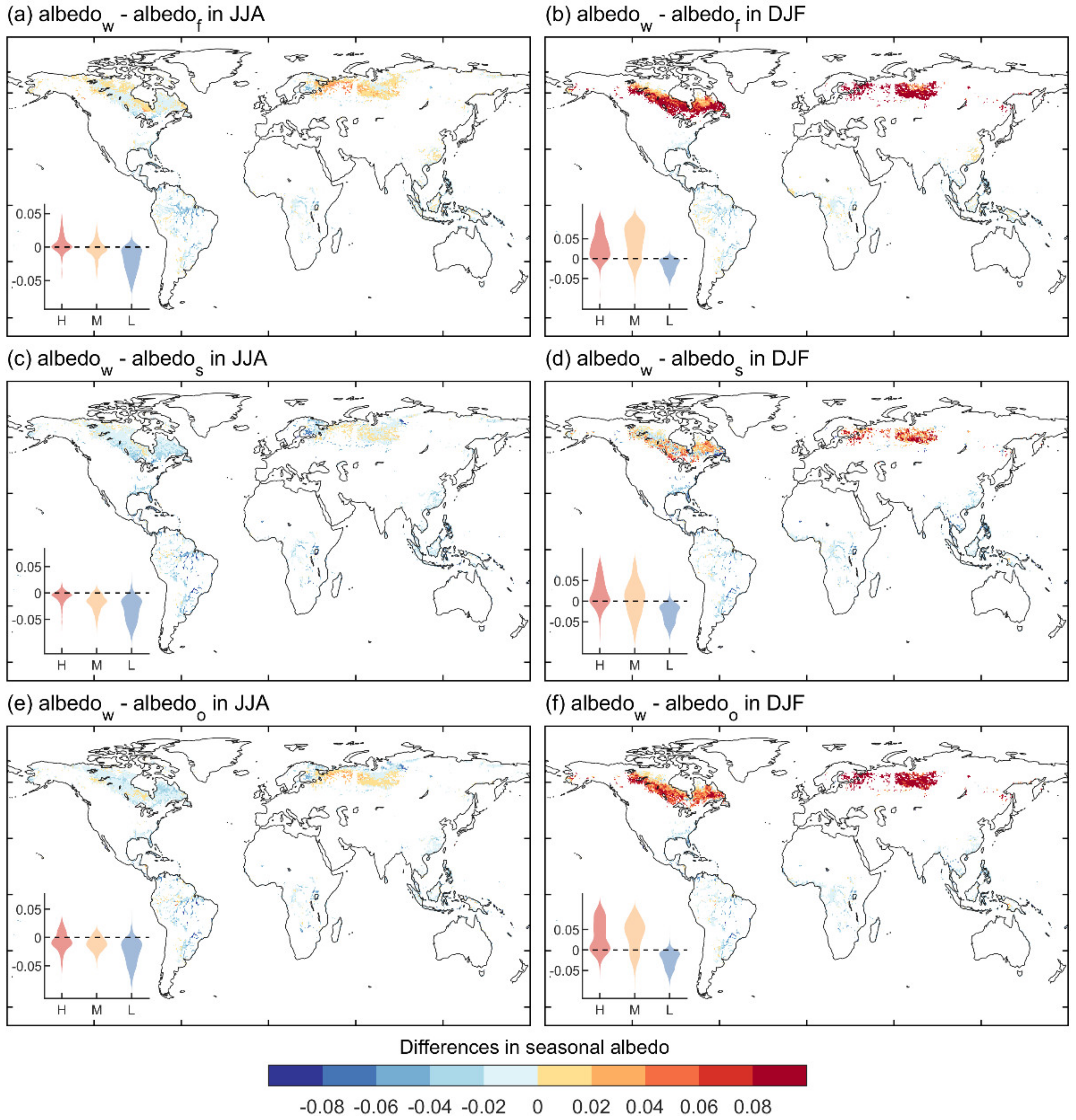
To illustrate the radiative and nonradiative impacts of wetlands on LST, the spatial patterns of seasonal Δalbedo and ΔET between wetlands and the other three landcover types were further investigated (Figure 4 and Figure 5). Figure 4 shows the spatial patterns of Δalbedo of JJA and DJF between wetlands and forests ( Δ albedo f w , Figure 4a,b), wetlands and shrublands ( Δ albedo s w , Figure 4c,d) and wetlands and open lands ( Δ albedo o w , Figure 4e,f). Δalbedo of MAM and SON are shown in Figure S4. In tropical regions, Δalbedo (i.e., Δ albedo f w , Δ albedo s w and Δ albedo o w were all negative (i.e., −0.02 ± 0.02, −0.03 ± 0.03, and −0.03 ± 0.02, respectively) throughout the year, indicating that wetlands had a smaller albedo and thus reflected less solar radiation than the other three landcover types. However, in the boreal regions, Δalbedo had different signals between summer and winter. In summer, the mean of Δalbedo was close to zero (i.e., 0.00 ± 0.02, −0.01 ± 0.02, and −0.01 ± 0.02) for Δ albedo f w , Δ albedo s w and Δ albedo o w , respectively), while in winter, the Δalbedo values were all positive (i.e., 0.12 ± 0.1, 0.02 ± 0.04, and 0.08 ± 0.07 for Δ albedo f w , Δ albedo s w and Δ albedo o w respectively) (Figure 4b,d,f). This indicates that wetlands have a higher albedo in winter due to snow cover [18,31] and thus reflect more solar radiation than the other three landcover types.
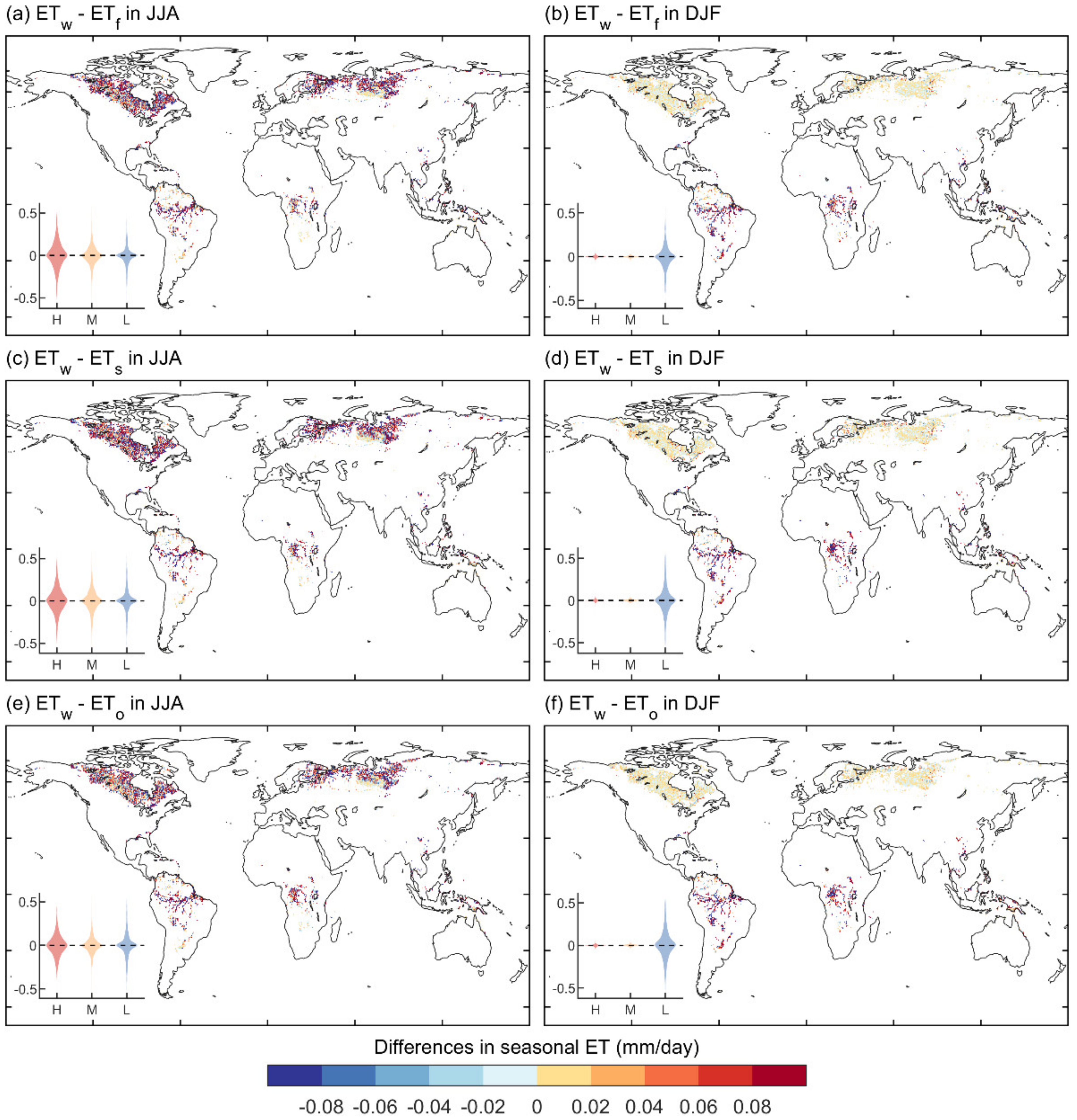
Figure 5 shows the spatial pattern of ΔET of JJA and DJF between wetlands and forests ( Δ ET f w , Figure 5a,b), wetlands and shrublands ( Δ ET s w , Figure 5c,d), and wetlands and open lands ( Δ ET o w , Figure 5e,f). ΔET of MAM and SON are shown in Figure S5. Similar to Δalbedo, in tropical regions, ΔET had an almost consistent pattern throughout the year, while in the boreal regions ΔET had distinct patterns between summer and winter. Specifically, in tropical regions, ΔET had similar values (i.e., 0.00 ± 0.20, 0.00 ± 0.25, and 0.01 ± 0.28 mm/day for Δ ET f w , Δ ET s w and Δ ET o w , respectively) and had little seasonality. In boreal regions, although ΔET had negative values throughout the year; the absolute values of ΔET decreased as the season shifted from summer (0.00 ± 0.18 mm/day) to winter (0.01 ± 0.02 mm/day).

4. Discussion

4.1. The Cooling or Warming Effect of Wetlands

The global pattern of ΔLST between wetlands and other landcover types provides an important insight that the overall behavior of wetlands throughout the year has a warming effect in boreal regions but a cooling effect in the tropical regions. Many local scale studies located in different regions confirm the global spatial patterns in ΔLST found in our results. For example, in tropical regions, the similar cooling effect (−1.7 °C) of wetlands is observed in the Minjiang River (25°N–26°N, 119°E–120°E) by comparing the satellite-based LST over wetlands and other adjacent landscapes from 1993–2013 [32]. In the Kilombero catchment (7°S–10°S, 34°E–37°E), from 2000 to 2017, the shrinking of wetlands increased the MODIS LST of the corresponding grid cell by 2–3 °C [33]. In temperate regions, in a three-year (2015–2017) observation of the eddy flux tower, it was found that the annual aerodynamic surface temperature of wetlands was up to 0.2 °C warmer than that of adjacent croplands in the Sacramento–San Joaquin Delta, California, USA [14]. In boreal regions, the annual warming effects of wetlands were seldom reported in previous case studies, probably due to the warming or cooling effect of wetlands being only observed in the growing season or summer. Seasonally, we find that ΔLST indicates a cooling effect of wetlands in summer but a warming effect in winter, which could be supported by several reported cases. In Northern Wisconsin, USA, using 2.4m air temperature observations of the eddy flux tower, Turner et al. indicated that the wetlands with more sedge meadow and forests (i.e., sheltered fens) had a stronger cooling effect than wetlands with less vegetation (i.e., open fens) due to the lower latent heat flux of the latter during the growing season [34]. The warming effect in winter was confirmed in a three-year (2015–2017) observation of eddy flux tower data which showed that the LST of wetlands was up to 0.73 °C higher than that of adjacent croplands in the Sacramento–San Joaquin Delta, California, USA [14]. Our satellite-based methods found the ΔLST ranging from –1.08 to 0.65 °C, indicating large spatial heterogeneity of ΔLST around the world. This warns that site-level observation of ΔLST may under- or overrepresent the large-scale impact of wetlands on local LST.

4.2. Mechanisms of the Warming or Cooling Effects of Wetlands

The spatial patterns of ΔLST (i.e., LST f w , LST s w , and LST o w ) can be interpreted by the surface energy budget as Equation (1) [15]. ΔS in the ecosystem is the chemical energy produced through photosynthesis and the temperature increase of the plant biomass [11]. The energy of ΔS is generally less than 5% of the net shortwave radiation [15]. In our study, the difference of ΔS between wetlands and other landcover types could be estimated by difference in gross primary production (ΔGPP) as chemical energy fixed through photosynthesis. The ΔGPP between adjacent different biomass was less than 2 g C m−2 day−1 [35], equal to ~80 kJ m−2 day−1 (0.9 W m−2). Thus, the difference in ΔS between wetlands and other landcover types was less than 1% of energy derived from ΔET and Δalbedo, and was neglected in our study. By neglecting the ecosystem chemical energy variation ΔS’ in Equation (2), Figure 6 shows the difference in surface energy budget between wetlands and other adjacent landcover types for summer and winter. Generally, ΔH was highly positively correlated with ΔLST [11], and ΔK and ΔLE were generally regarded as the two major energy fluxes to explain ΔH.
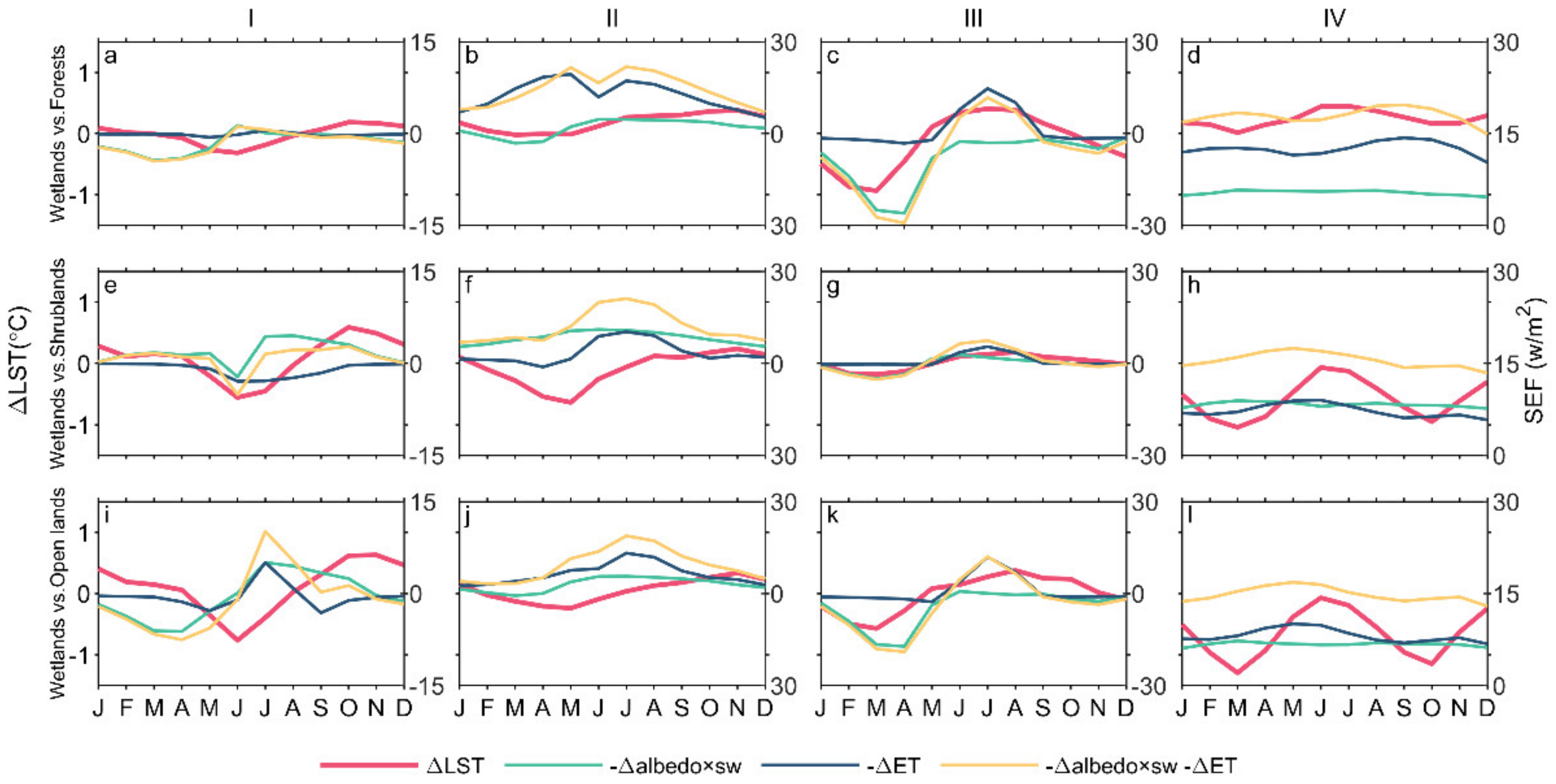
To be more intuitive, the contributions of Δalbedo and ΔET to ΔLST in the entire seasonal cycle as well as in two seasons (i.e., summer and winter) are identified in Figure 7. In tropical regions, the contributions of the Δalbedo and ΔET indicated a slight difference between summer (Figure 7d–f) and winter (Figure 7g–i) which explains the little seasonality of ΔLST; whereas in boreal regions, in winter, the contribution of Δalbedo was much higher than that of ΔET (Figure 7e,f). In summer, the contributions Δalbedo and ΔET to ΔLST were comparable (Figure 7c,d). Throughout the multiple years, 30% of temporal variation in ΔLST can be attributed to Δalbedo and ΔET together, with their contributions being respectively 20% and 10% (Figure 7a–c). This suggests that in wetlands, other factors (e.g., G) may play a more important part in ΔLST. To better interpret the contributions of Δalbedo and ΔET to ΔLST in different regions, Figure 8 compares the seasonal cycle of mean values of ΔLST and involved surface energy fluxes for typical regions I, II, III, and IV. In West Siberia (Region III), the seasonal cycle of ΔLST matched well with that of ΔSEF (i.e., the energy fluxes derived from Δalbedo and ΔET) (Figure 8c,g,h), suggesting that the ΔLST between wetlands and other landcover types can be well interpreted by the corresponding Δalbedo and ΔET in typical region III. In Canada, however, ΔLST started to increase in May and June and reached its peak in October and November, which was approximately 4~6 months later than the peak of ΔSEF (around June). A similar seasonal cycle of ΔLST was confirmed in three-year in situ observations in three different wetlands [14]. As ΔL can be calculated by multiplying the difference of the fourth power of wetlands’ and other landcover types’ LST by the Stefan–Boltzmann constant 5.67 × 10⁻⁸ W m−2 K−4, ΔL is up to 2.5 W/m2 when the LST is 20 °C in the tropical regions and ΔLST is 0.7 °C. This is much smaller than ΔSEF so that ΔL is negligible. Here, we hypothesize that the time lag between the peaks of ΔLST and ΔSEF can be attributed to the seasonality of ground heat flux (G), as wetlands can store more energy in summer and then release it in winter due to larger water storage and the larger specific heat capacity of water (4200 J/Kg/°C) compared to soils (~2500 J/Kg/°C) [36]. Region I and II (northern and southern Canada) have a lot of wetlands including large lakes (e.g., the Great Lakes) that store plentiful water [37]. By in situ meteorological measurements, G of wetlands (14 W m−2 ) is two times higher than G of adjacent pasture during the growing season in the Třeboň Biosphere Reserve in southern Bohemia (48°49′–49°20′N, 14°39′–15°00′E) [38]. Global G has been modeled such that in the boreal regions, the highest G is found in summer at 19 W/m2, while the lowest G is in winter at −17 W/m2 [39]. This confirms that the ground absorbs energy in summer and releases it in winter. However, the lack of large-scale ground flux G data hinders the interpretation of global patterns of ΔLST in different seasons, which needs further efforts. Besides, in tropical regions (IV), with their dense vegetation cover, the landcover maps have difficulty in distinguishing wetlands under forests (e.g., swamps) and tropical forests [40]. Consequently, ΔLST calculated in tropical regions (IV) based on satellite products in this study has a large degree of uncertainty, and ΔLST data in tropical regions (IV) should be interpreted with caution. Our study investigates the warming or cooling effects of wetlands and provides a cohesive picture of the difference of summer and winter surface heat budgets between wetlands and other landcover types (Figure 6). Generally, wetlands had a larger absolute value of LE in summer than other landcover types while receiving less net shortwave radiation in winter due to more snow cover. The wetlands absorbed more energy (G) down to the ground than other landcover types in summer while releasing more energy in winter.

5. Conclusions

In this study, using satellite-based datasets, we show the global patterns of annual and seasonal ΔLST between wetlands and other landcover types, as well as Δalbedo and ΔET. Our results show that in the tropical regions, the annual LST of wetlands are lower than those in forest, shrubland and open land; i.e., in these regions wetlands have a cooling effect while in the boreal regions, the wetlands have a warming effect. While ΔLST in the tropical regions has little seasonality, in the boreal regions, wetlands have a cooling effect in summer but a warming effect in winter. Only 30% of the spatial patterns of ΔLST and their seasonal variations can be attributed to the Δalbedo and ΔET in west Siberia. The remaining part of ΔLST that cannot be interpreted by Δalbedo and ΔET can be attributed to the ground heat flux, G, for instance in Canada, which can also interpret the time lag of the peaks of ΔLST and involved surface energy fluxes. Nowadays, there is an increasing interest in wetland restoration for mitigating climate change. Wetland restoration could greatly reduce nitrogen pollution [41], and methane and CO2 emission [42], as well as change the local biophysical processes. This study highlights the potential climatic benefits of widespread wetland restoration in the future. As wetlands in different regions have different climatic effects (warming or cooling local temperature), there should be careful consideration of climatic benefits of wetland restoration in different regions.

Supplementary Materials

The following are available online at https://www.mdpi.com/article/10.3390/rs13081439/s1, Table S1: Statistics of ΔLST, Δalbedo, and ΔET in four regions; Figure S1: Spatial patterns of mean annual air temperature and LST of wetlands; Figure S2: Spatial patterns of mean annual albedo of wetlands; Figure S3: Differences in seasonal LST between wetlands, forests, and open lands; Figure S4: Differences in seasonal albedo between wetlands, forests, and open lands; Figure S5: Differences in seasonal ET between wetlands, forests, and open lands.

Author Contributions

Data analysis and interpretation was conducted primarily by Y.W.; writing—original draft preparation, Y.W.; writing—review and editing, Y.X., M.F. and S.P. This study was designed by S.P. All authors have read and agreed to the published version of the manuscript.

Funding

This research was funded by the National Natural Science Foundation of China, grant number 41830643, and the National Key Research and Development Program of China, grant number 2016YFA0600202. Funding for this study was provided by undergraduate student research training program of the Ministry of Education.

Data Availability Statement

The MODIS products are available from EARTHDATA (https://lpdaac.usgs.gov/products/, accessed on 11 November 2018). The CERES–EBAF shortwave fluxes are available from CERES (https://ceres.larc.nasa.gov/data/, accessed on 10 May 2019). The CRU TS v.4.02 climate datasets are available from CRU (https://crudata.uea.ac.uk/cru/data/hrg/cru_ts_4.02/, accessed on 11 November 2018).

Acknowledgments

This study was supported by High-performance Computing Platform of Peking University.

Conflicts of Interest

The authors declare no conflict of interest.

References

  1. Tootchi, A.; Jost, A.; Ducharne, A. Multi-source global wetland maps combining surface water imagery and groundwater constraints. Earth Syst. Sci. Data 2019, 11, 189–220. [Google Scholar] [CrossRef] [Green Version]
  2. Zedler, J.B.; Kercher, S. Wetland resources: Status, trends, ecosystem services, and restorability. Annu. Rev. Environ. Resour. 2005, 30, 39–74. [Google Scholar] [CrossRef] [Green Version]
  3. Finlayson, M.; Cruz, R.D.; Davidson, N.; Alder, J.; Cork, S.; de Groot, R.S.; Lévêque, C.; Milton, G.R.; Peterson, G.; Pritchard, D.; et al. Millennium Ecosystem Assessment: Ecosystems and Human Well-Being: Wetlands and Water Synthesis; Island Press: Washington, DC, USA, 2005. [Google Scholar]
  4. Gardner, R.; Finlayson, M. Global Wetland Outlook: State of the World’s Wetlands and their Services to People; Ramsar: Gland, Switzerland, 2018. [Google Scholar]
  5. Russi, D.; ten Brink, P.; Farmer, A.; Badura, T.; Coates, D.; Förster, J.; Kumar, R.; Davidson, N. The Economics of Ecosystems and Biodiversity for Water and Wetlands; IEEP: Bruxelles, Belgium, 2012. [Google Scholar]
  6. Prigent, C.; Jimenez, C.; Bousquet, P. Satellite-Derived Global Surface Water Extent and Dynamics Over the Last 25 Years (GIEMS-2). J. Geophys. Res. Atmos. 2020, 125, 125. [Google Scholar] [CrossRef]
  7. Jensen, K.; McDonald, K. Surface Water Microwave Product Series Version 3: A Near-Real Time and 25-Year Historical Global Inundated Area Fraction Time Series From Active and Passive Microwave Remote Sensing. IEEE Geosci. Remote Sens. Lett. 2019, 16, 1402–1406. [Google Scholar] [CrossRef]
  8. Prigent, C.; Papa, F.; Aires, F.; Jimenez, C.; Rossow, W.B.; Matthews, E. Changes in land surface water dynamics since the 1990s and relation to population pressure. Geophys. Res. Lett. 2012, 39, L08403. [Google Scholar] [CrossRef] [Green Version]
  9. UN. General Assembly Resolution A/RES/70/1. Transforming Our World, the 2030 Agenda for Sustainable Development; UN: New York, NY, USA, 2015. [Google Scholar]
  10. Xu, X.; Chen, M.; Yang, G.; Jiang, B.; Zhang, J. Wetland ecosystem services research: A critical review. Glob. Ecol. Conserv. 2020, 22, e01027. [Google Scholar] [CrossRef]
  11. Chapin, F.S., III; Matson, P.A.; Vitousek, P. Principles of Terrestrial Ecosystem Ecology, 2nd ed.; Springer: New York, NY, USA, 2011. [Google Scholar]
  12. Sumner, D.M.; Wu, Q.; Pathak, C.S. Variability of Albedo and Utility of the MODIS Albedo Product in Forested Wetlands. Wetlands 2011, 31, 229–237. [Google Scholar] [CrossRef]
  13. Georg, W.; Albin, H.; Georg, N.; Katharina, S.; Enrico, T.; Peng, Z. On the energy balance closure and net radiation in complex terrain. Agric. For. Meteorol. 2016, 226-227, 37–49. [Google Scholar] [CrossRef] [PubMed] [Green Version]
  14. Hemes, K.S.; Eichelmann, E.; Chamberlain, S.D.; Knox, S.H.; Oikawa, P.Y.; Sturtevant, C.; Verfaillie, J.; Szutu, D.; Baldocchi, D.D. A Unique Combination of Aerodynamic and Surface Properties Contribute to Surface Cooling in Restored Wetlands of the Sacramento-San Joaquin Delta, California. J. Geophys. Res. Biogeosci. 2018, 123, 2072–2090. [Google Scholar] [CrossRef]
  15. Worrall, F.; Boothroyd, I.M.; Gardner, R.L.; Howden, N.J.K.; Burt, T.P.; Smith, R.; Mitchell, L.; Kohler, T.; Gregg, R. The Impact of Peatland Restoration on Local Climate: Restoration of a Cool Humid Island. J. Geophys. Res. Biogeosci. 2019, 124, 1696–1713. [Google Scholar] [CrossRef]
  16. Bai, J.; Lu, Q.; Zhao, Q.; Wang, J.; Ouyang, H. Effects of Alpine Wetland Landscapes on Regional Climate on the Zoige Plateau of China. Adv. Meteorol. 2013, 2013, 1–7. [Google Scholar] [CrossRef]
  17. Zheng, H.Z.; Chen, Y.H.; Pan, W.B.; Zheng, P.; Cai, Y.B. Land surface temperature fluctuation characteristics and key influencing factors in estuarine wetland. Shengtaixue Zazhi 2018, 37, 2463–2473. [Google Scholar]
  18. Peng, S.-S.; Piao, S.; Zeng, Z.; Ciais, P.; Zhou, L.; Li, L.Z.X.; Myneni, R.B.; Yin, Y.; Zeng, H. Afforestation in China cools local land surface temperature. Proc. Natl. Acad. Sci. USA 2014, 111, 2915–2919. [Google Scholar] [CrossRef] [PubMed] [Green Version]
  19. Li, Y.; Zhao, M.; Motesharrei, S.; Mu, Q.; Kalnay, E.; Li, S. Local cooling and warming effects of forests based on satellite observations. Nat. Commun. 2015, 6, 6603. [Google Scholar] [CrossRef] [Green Version]
  20. Friedl, M.A.; Sulla-Menashe, D.; Tan, B.; Schneider, A.; Ramankutty, N.; Sibley, A.; Huang, X. MODIS Collection 5 global land cover: Algorithm refinements and characterization of new datasets. Remote Sens. Environ. 2010, 114, 168–182. [Google Scholar] [CrossRef]
  21. Wan, Z.; Dozier, J. A generalized split-window algorithm for retrieving land-surface temperature from space. IEEE Trans. Geosci. Remote. Sens. 1996, 34, 892–905. [Google Scholar] [CrossRef] [Green Version]
  22. Lian, X.; Zeng, Z.; Yao, Y.; Peng, S.; Wang, K.; Piao, S. Spatiotemporal variations in the difference between satellite-observed daily maximum land surface temperature and station-based daily maximum near-surface air temperature. J. Geophys. Res. Atmos. 2017, 122, 2254–2268. [Google Scholar] [CrossRef]
  23. Wan, Z. New refinements and validation of the collection-6 MODIS land-surface temperature/emissivity product. Remote. Sens. Environ. 2014, 140, 36–45. [Google Scholar] [CrossRef]
  24. Mira, M.; Weiss, M.; Baret, F.; Courault, D.; Hagolle, O.; Gallego-Elvira, B.; Olioso, A. The MODIS (collection V006) BRIDF/albedo product MCD43D: Temporal course evaluated over agricultural landscape. Remote Sens. Environ. 2015, 170, 216–228. [Google Scholar] [CrossRef] [Green Version]
  25. Cescatti, A.; Marcolla, B.; Vannan, S.K.S.; Pan, J.Y.; Román, M.O.; Yang, X.; Ciais, P.; Cook, R.B.; Law, B.E.; Matteucci, G.; et al. Intercomparison of MODIS albedo retrievals and in situ measurements across the global FLUXNET network. Remote Sens. Environ. 2012, 121, 323–334. [Google Scholar] [CrossRef] [Green Version]
  26. Kalma, J.D.; McVicar, T.R.; Matthew, F. UNSW Faculty of Engineering Matthew Francis McCabe Estimating Land Surface Evaporation: A Review of Methods Using Remotely Sensed Surface Temperature Data. Surv. Geophys. 2008, 29, 421–469. [Google Scholar] [CrossRef]
  27. Kim, H.W.; Hwang, K.; Mu, Q.; Lee, S.O.; Choi, M. Validation of MODIS 16 global terrestrial evapotranspiration products in various climates and land cover types in Asia. KSCE J. Civ. Eng. 2012, 16, 229–238. [Google Scholar] [CrossRef]
  28. Harris, I.; Osborn, T.J.; Jones, P.; Lister, D. Version 4 of the CRU TS monthly high-resolution gridded multivariate climate dataset. Sci. Data 2020, 7, 1–18. [Google Scholar] [CrossRef] [PubMed] [Green Version]
  29. Budescu, D.V. Dominance Analysis—A New Approach to the Problem of Relative Importance of Predictors in Multiple-Regression. Psychol. Bull. 1993, 114, 542–551. [Google Scholar] [CrossRef]
  30. Cui, E.; Huang, K.; Arain, M.A.; Fisher, J.B.; Huntzinger, D.N.; Ito, A.; Luo, Y.; Jain, A.K.; Mao, J.; Michalak, A.M.; et al. Vegetation Functional Properties Determine Uncertainty of Simulated Ecosystem Productivity: A Traceability Analysis in the East Asian Monsoon Region. Glob. Biogeochem. Cycles 2019, 33, 668–689. [Google Scholar] [CrossRef] [Green Version]
  31. Yu, L.; Liu, T.; Zhang, S. Temporal and Spatial Changes in Snow Cover and the Corresponding Radiative Forcing Analysis in Siberia from the 1970s to the 2010s. Adv. Meteorol. 2017, 2017, 1–11. [Google Scholar] [CrossRef] [Green Version]
  32. Zheng, H.; Chen, Y.; Pan, W.; Cai, Y.; Chen, Z. Impact of Land Use/Land Cover Changes on the Thermal Environment in Urbanization: A Case Study of the Natural Wetlands Distribution Area in Minjiang River Estuary, China. Pol. J. Environ. Stud. 2019, 28, 3025–3041. [Google Scholar] [CrossRef]
  33. Muro, J.; Strauch, A.; Heinemann, S.; Steinbach, S.; Thonfeld, F.; Waske, B.; Diekkrüger, B. Land surface temperature trends as indicator of land use changes in wetlands. Int. J. Appl. Earth Obs. Geoinf. 2018, 70, 62–71. [Google Scholar] [CrossRef]
  34. Turner, J.; Desai, A.R.; Thom, J.; Wickland, K.P.; Olson, B. Wind Sheltering Impacts on Land-Atmosphere Fluxes Over Fens. Front. Environ. Sci. 2019, 7, 179. [Google Scholar] [CrossRef]
  35. Xiao, J.; Zhuang, Q.; Law, B.E.; Chen, J.; Baldocchi, D.D.; Cook, D.R.; Oren, R.; Richardson, A.D.; Wharton, S.; Siyan USA (host institution) IN 47907 West Lafayette Purdue University Purdue Climate Change Research Center Department of Earth & Atmospheric Sciences. A continuous measure of gross primary production for the conterminous United States derived from MODIS and AmeriFlux data. Remote. Sens. Environ. 2010, 114, 576–591. [Google Scholar] [CrossRef] [Green Version]
  36. Wang, Y.; Lu, Y.; Horton, R.; Ren, T. Specific Heat Capacity of Soil Solids: Influences of Clay Content, Organic Matter, and Tightly Bound Water. Soil Sci. Soc. Am. J. 2019, 83, 1062–1066. [Google Scholar] [CrossRef]
  37. Lehner, B.; Döll, P. Development and validation of a global database of lakes, reservoirs and wetlands. J. Hydrol. 2004, 296, 1–22. [Google Scholar] [CrossRef]
  38. Huryna, H.; Brom, J.; Pokorný, J. The importance of wetlands in the energy balance of an agricultural landscape. Wetl. Ecol. Manag. 2013, 22, 363–381. [Google Scholar] [CrossRef]
  39. Tsuang, B.-J. Ground Heat Flux Determination according to Land Skin Temperature Observations from In Situ Stations and Satellites. J. Hydrometeorol. 2005, 6, 371–390. [Google Scholar] [CrossRef]
  40. Sulla-Menashe, D.; Gray, J.M.; Abercrombie, S.P.; Friedl, M.A. Hierarchical mapping of annual global land cover 2001 to present: The MODIS Collection 6 Land Cover product. Remote Sens. Environ. 2019, 222, 183–194. [Google Scholar] [CrossRef]
  41. Cheng, F.Y.; Van Meter, K.J.; Byrnes, D.K.; Basu, N.B. Maximizing US nitrate removal through wetland protection and restoration. Nat. Cell Biol. 2020, 588, 625–630. [Google Scholar] [CrossRef]
  42. Kroeger, K.D.; Crooks, S.; Moseman-Valtierra, S.; Tang, J. Restoring tides to reduce methane emissions in impounded wetlands: A new and potent Blue Carbon climate change intervention. Sci. Rep. 2017, 7, 1–12. [Google Scholar] [CrossRef] [PubMed] [Green Version]
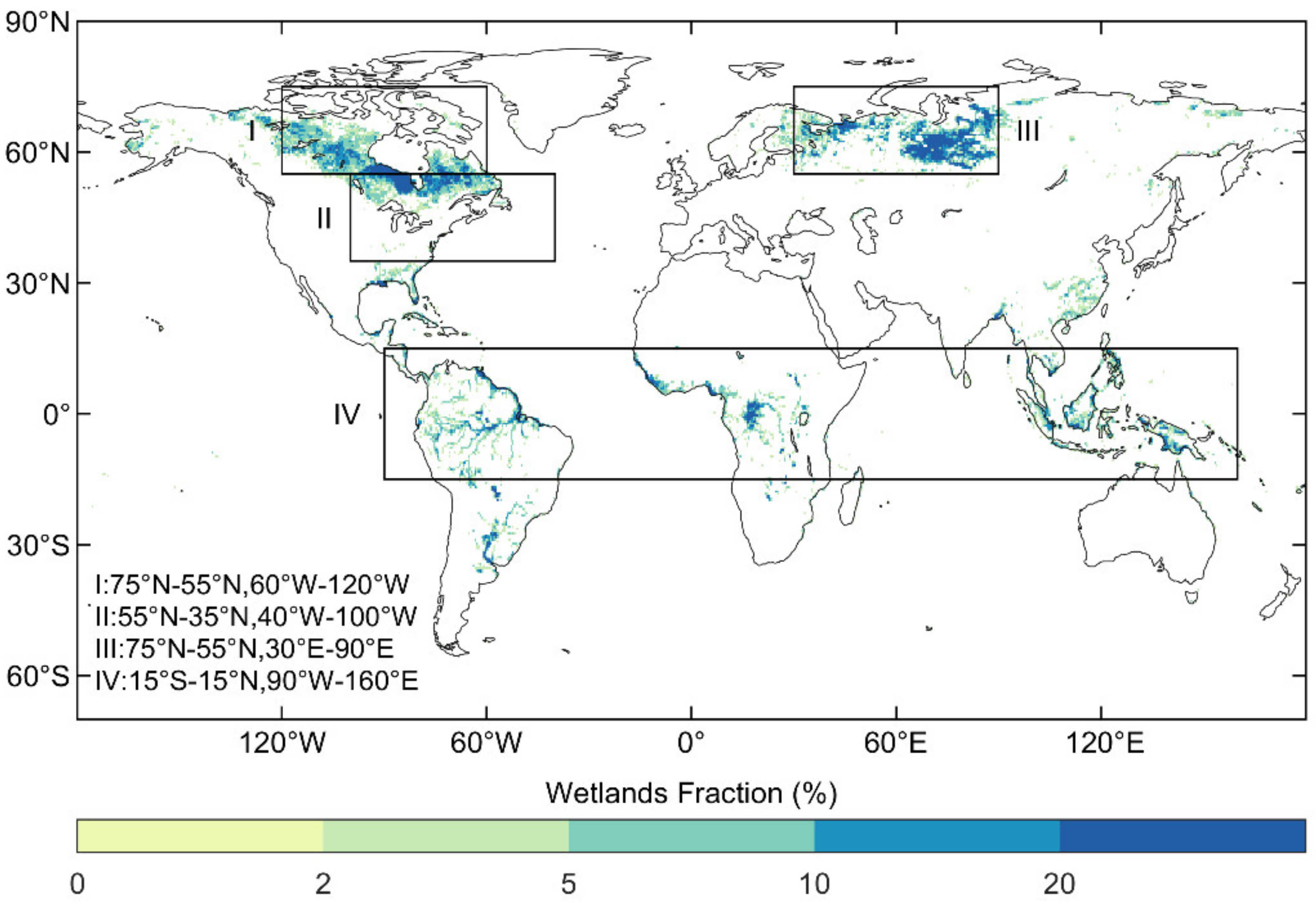
Figure 1. Spatial distribution of global wetlands.
Remotesensing 13 01439 g001
Figure 2. Spatial patterns of difference in land surface temperature (ΔLST) between wetlands and air temperature ( Δ LST a w ; a), ( Δ LST f w , Δ LST s w and Δ LST o w ) wetlands and forests ( Δ LST f w ; b), wetlands and shrublands ( Δ LST s w ; c), and wetland and open lands ( Δ LST o w ; d) during the period 2001–2017. Regions labeled by black dots indicate values that are statistically significantly positive or negative (t-test; p < 0.05). In each subplot, the violin plot in the left-bottom panel summarizes the statistics in the high-latitude (>60°N, denoted by H), middle-latitude (30°N–60°N, denoted by M), and low-latitude (30°S–30°N, denoted by L) regions.
Remotesensing 13 01439 g002
Figure 3. Spatial patterns of ΔLST between wetlands and forests ( Δ LST f w ; a,b), wetlands and shrubs ( Δ LST s w ; c,d), and wetlands and open landscape ( Δ LST o w ; e,f) in summer (a,c,e) and winter (b,d,f). In each subplot, the violin plot in the left-bottom panel summarizes the statistics in the high-latitude (>60°N, denoted by H), middle-latitude (30°N–60°N, denoted by M), and low-latitude (30°S–30°N, denoted by L) regions.
Remotesensing 13 01439 g003
Figure 4. Spatial patterns of difference in albedo (Δalbedo) between wetlands and forests ( Δ albedo f w ; a,b), wetlands and shrubs ( Δ albedo s w ; c,d), and wetlands and open land ( Δ albedo o w ; e,f) in summer (a,c,e) and winter (b,d,f). In each subplot, the violin plot in the left-bottom panel summarizes the statistics in the high-latitude (>60°N, denoted by H), middle-latitude (30°N–60°N, denoted by M), and low-latitude (30°S–30°N, denoted by L) regions.
Remotesensing 13 01439 g004
Figure 5. Spatial patterns of difference in evapotranspiration (ΔET) between wetlands and forests ( Δ ET f w ; a,b), wetlands and shrubs ( Δ ET s w ; c,d), and wetlands and open land ( Δ ET o w ; e,f) in summer (a,c,e) and winter (b,d,f). In each subplot, the violin plot in the left-bottom panel summarizes the statistics in the high-latitude (>60°N, denoted by H), middle-latitude (30°N–60°N, denoted by M), and low-latitude (30°S–30°N, denoted by L) regions.
Remotesensing 13 01439 g005
Figure 6. Comparing surface heat budgets between wetlands and other landcover types in summer (a) and winter (b). In each panel, the surface heat budgets include shortwave radiation (ΔSW), longwave radiation (ΔLW), sensible heat flux (ΔH), latent heat flux (ΔLE), and ground heat flux (ΔG).
Remotesensing 13 01439 g006
Figure 7. Relative contributions of Δalbedo and ΔET to ΔLST in the entire seasonal cycle (ac), and in summer (df), and winter (gi).
Remotesensing 13 01439 g007
Figure 8. Seasonal cycle of the mean values of ΔLST and surface energy flux (SEF). Columns 1, 2, 3, 4 correspond to typical regions (IIV), respectively; rows 1, 2, 3 correspond to the LST f w , LST s w , and LST o w , respectively.
Remotesensing 13 01439 g008
Table 1. The extent of each landcover type from the classification.
NumberClassExtent
(Million km2)
Percentage of the Land SurfaceIGBP
1Wetland1.10.7%Permanent Wetlands
2Forest22.314.9%Evergreen needleleaf forests, evergreen broadleaf forests, deciduous needleleaf forests, deciduous broadleaf forest, mixed forests
3Shrubland3926.2%Closed shrublands, open shrublands, woody savannas, savannas
4Open land34.523.1%Grasslands, croplands, cropland—natural vegetation mosaic
Publisher’s Note: MDPI stays neutral with regard to jurisdictional claims in published maps and institutional affiliations.