Article

A Large-Scale Deep-Learning Approach for Multi-Temporal Aqua and Salt-Culture Mapping

by
Cesar Diniz
1,2,*,
Luiz Cortinhas
1,3,
Maria Luize Pinheiro
1,3,
Luís Sadeck
1,4,
Alexandre Fernandes Filho
1,5,
Luis R. F. Baumann
6,
Marcos Adami
2,7 and
Pedro Walfir M. Souza-Filho
2,8
1
Solved—Solutions in Geoinformation, Belém 66075-750, Brazil
2
Geoscience Institute, UFPA—Federal University of Pará, Belém 66075-110, Brazil
3
Technology Institute, UFPA—Federal University of Pará, Belém 66075-110, Brazil
4
Philosophy and Human Sciences Institute, UFPA—Federal University of Pará, Belém 66075-110, Brazil
5
Institute of Agricultural Sciences, UFRA—Federal Rural University of the Amazon, Belém 66077-813, Brazil
6
Institute of Mathematics and Statistics, UFG—Federal University of Goias, Goiania 74690-900, Brazil
7
INPE—National Institute for Space Research, Amazon Spatial Coordination, São Paulo 12227-010, Brazil
8
ITV—Instituto Tecnológico Vale, Belém 66055-090, Brazil
*
Author to whom correspondence should be addressed.
Remote Sens. 2021, 13(8), 1415; https://doi.org/10.3390/rs13081415
Submission received: 25 February 2021 / Revised: 31 March 2021 / Accepted: 31 March 2021 / Published: 7 April 2021
(This article belongs to the Special Issue State-of-the-Art Remote Sensing in South America)

Abstract

:
Aquaculture and salt-culture are relevant economic activities in the Brazilian Coastal Zone (BCZ). However, automatic discrimination of such activities from other water-related covers/uses is not an easy task. In this sense, convolutional neural networks (CNN) have the advantage of predicting a given pixel’s class label by providing as input a local region (named patches or chips) around that pixel. Both the convolutional nature and the semantic segmentation capability provide the U-Net classifier with the ability to access the “context domain” instead of solely isolated pixel values. Backed by the context domain, the results obtained show that the BCZ aquaculture/saline ponds occupied ~356 km2 in 1985 and ~544 km2 in 2019, reflecting an area expansion of ~51%, a rise of 1.5× in 34 years. From 1997 to 2015, the aqua-salt-culture area grew by a factor of ~1.7, jumping from 349 km2 to 583 km2, a 67% increase. In 2019, the Northeast sector concentrated 93% of the coastal aquaculture/salt-culture surface, while the Southeast and South sectors contained 6% and 1%, respectively. Interestingly, despite presenting extensive coastal zones and suitable conditions for developing different aqua-salt-culture products, the North coast shows no relevant aqua or salt-culture infrastructure sign.

1. Introduction

Aquaculture is the farming of aquatic organisms, including fish, mollusks, crustaceans, and aquatic plants. In this sense, farming implies some form of intervention in the rearing process to enhance production, such as regular stocking, feeding, and predators’ protection. Farming also presupposes individual or corporate ownership of the stock being cultivated [1].
Currently, half of the fish and mollusks used to feed the world’s population comes from aquaculture [2], and the world’s appetite for fish and fish products shows no sign of slowing. From 1990 to 2018, there was a ~14% rise in global capture fisheries, a 527% rise in aquaculture production, and a 122% rise in total food fish consumption [3].
Sharing similar characteristics with the aquaculture infrastructure, such as the exploitation of water resources, the need for artificial water-reservoir, and the dependency on coastal environments, the sea salt culture is another relevant economic activity in the Brazilian Coastal Zone (BCZ). Therefore, mapping aquaculture and salt-culture areas is a fundamental challenge for understanding the expansion of such activities and the sustainable management of these global coastal resources.
Aquaculture and salines have been mainly associated with valuable fertile environments and may be the origin of large-scale land-use changes. Due to their water-dependent nature, coastal aquaculture and saline activity require special attention, being directly associated with the loss of natural coastal wetlands and pollution of waters and soils [4]. Other studies have relayed on remote sensing images to understand the dynamics of classical coastal features such as mangroves, beaches, estuaries, and shoreline analysis [5,6,7,8,9,10,11,12,13]. However, there are fewer large-scale studies exhaustively identifying coastal aquaculture and salines, whether on the global or regional scale and yet, none rely on deep-learning algorithms [14,15].
The primary difficulty in automatically distinguishing between aqua or salt-culture and any other surface water target (e.g., rivers, lakes, or coastal waters) is the spectral similarity between them all. Spectrally speaking, water is water and, unless it presents a high concentration of optically active compounds (e.g., suspended sediments, algae, organic matter, and others), not much can be done to spectrally discriminate a variety of water-dependent targets [16,17,18,19]. In cases like this, when the natural cover among the targets to be set apart is the same, the context domain, rather than the spectral or temporal one, may hold the key to distinguish between rivers, lakes, natural or artificial ponds, and coastal water pixels.
In this scenario, the U-Net convolutional network [20] has the advantage of predicting the class label of each pixel by providing as input a local region (named patches or chips) around that given pixel. Such labeling characteristics, together with its convolutional nature and the semantic segmentation capability, provide the U-Net with the ability to access the “context domain” instead of solely isolated pixel values.
This research tests the application of a U-Net classifier over the BCZ, a coastal extension of ~9000 km, to assess its robustness in the multitemporal discrimination of artificial coastal ponds of aqua and salt-culture. The region presents a great diversity of coastal environments, such as mangroves, salt-flats, beaches, dunes, and coastal waters (e.g., estuaries, deltas, and tidal rivers) that influence the organization and spatial distribution of coastal aquaculture [8,21,22,23,24,25]. All this variability and complexity make the BCZ an appropriate region to evaluate the proposed method’s robustness. This paper aims to present, describe, and assess an Earth Engine-TensorFlow pipeline based on a U-Net large-scale deep-learning approach. The pipeline has been designed to classify artificial coastal ponds to pave the understanding of the aqua-salt-culture dynamics in the BCZ, based on 34 years of Landsat time-series data, from 1985 to 2019.

2. Materials and Methods
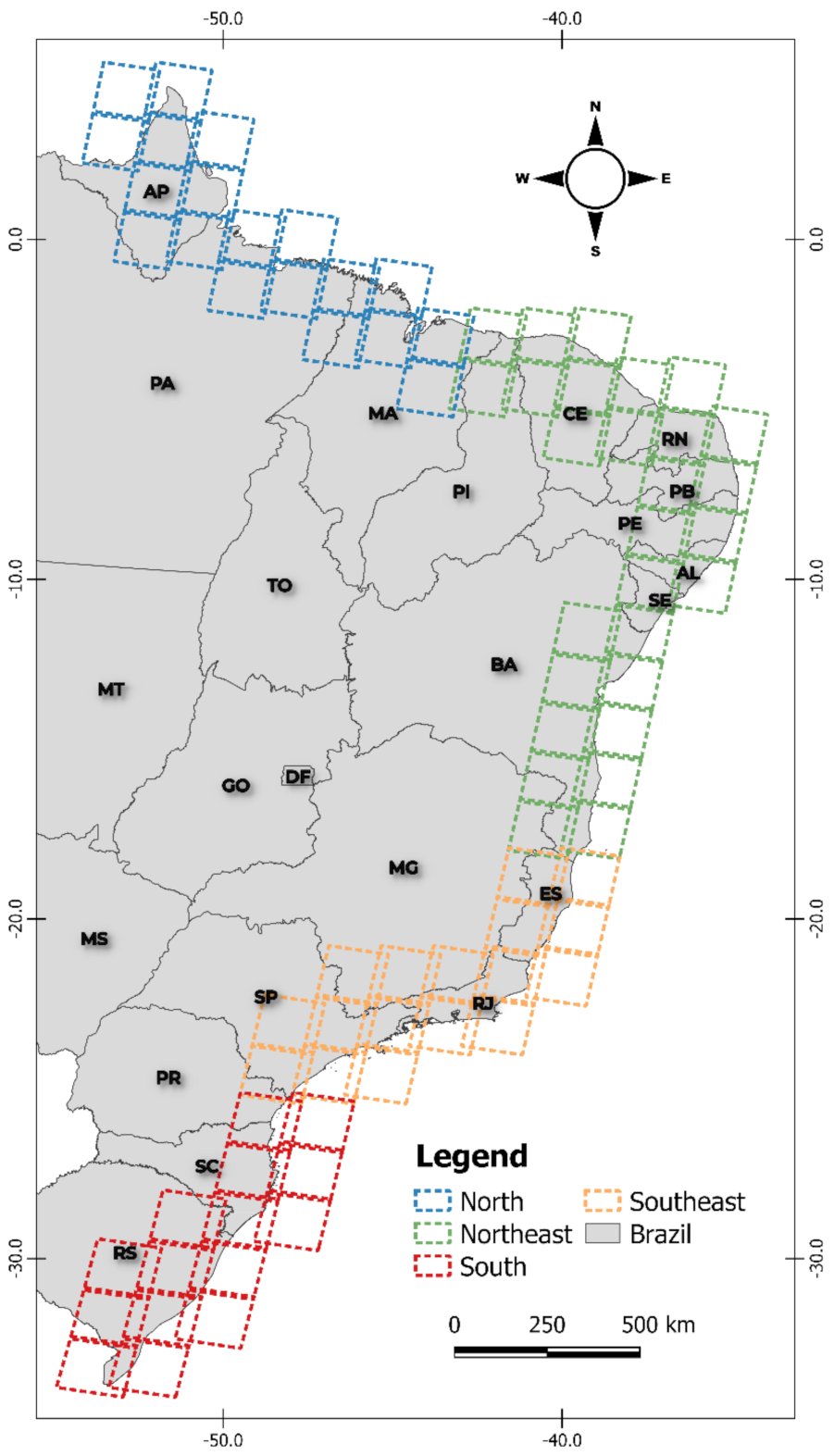
2.1. Study Site

In Brazil, between 2013 and 2018, aquaculture activity production increased by ~18%, jumping from 476 tons to 576 tons [26]. The Northeast and South regions lead the national aquaculture production; together, these regions are responsible for ~56% of the domestic market [26]. Compared to the global scenario, the experiment rate of increase can be considered relatively low, a characteristic that may be associated with the rapid expansion of white spot syndrome disease (WSSD), especially in the northeastern region of the country [27,28,29].
From a diversity perspective, Brazilian aquaculture is primarily dominated by fish farming, followed by shrimp farming, and finally by bivalve culture (oysters, scallops, and mussels). In 2018, these three crops represented near 89%, 8%, and 2% of national production, respectively [26]. While fish farms are widely spread throughout the country, shrimp farming and bivalve culture are mostly concentrated in the Northeast and South regions, respectively [30,31,32,33,34].
Together with traditional aquaculture, sea salt-culture is also common in the BCZ. Based on the evaporation of saline reservoirs’, this activity is responsible for 81% of Brazil’s salt production. Sea salt production is mainly associated with three states: Rio Grande do Norte (RN), Ceará (CE), and Rio de Janeiro (RJ) [4,5]. In 2017, 6 Mt of sea salt was produced in Brazil, 95% in RN, 3% from RJ, and another 1.5% from CE [5]. To better present the achieved results, the BCZ was divided into four regional sectors; North, Northeast, Southeast, and South (Figure 1).

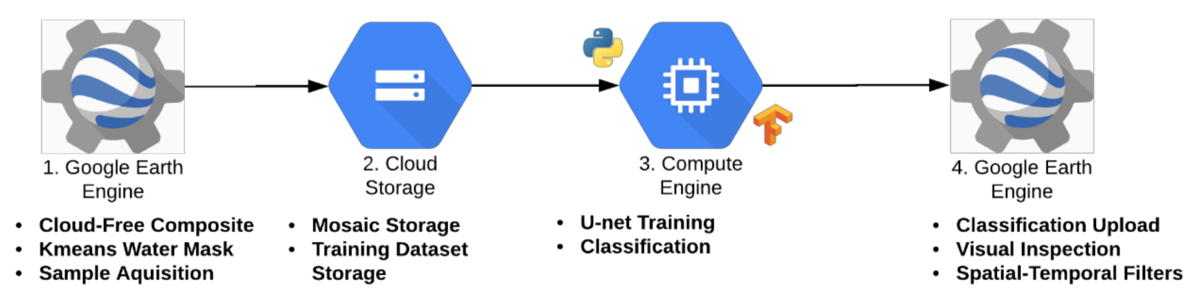
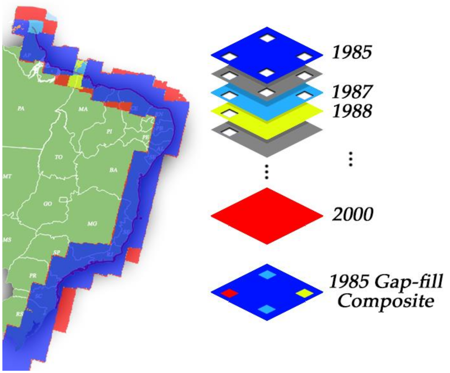
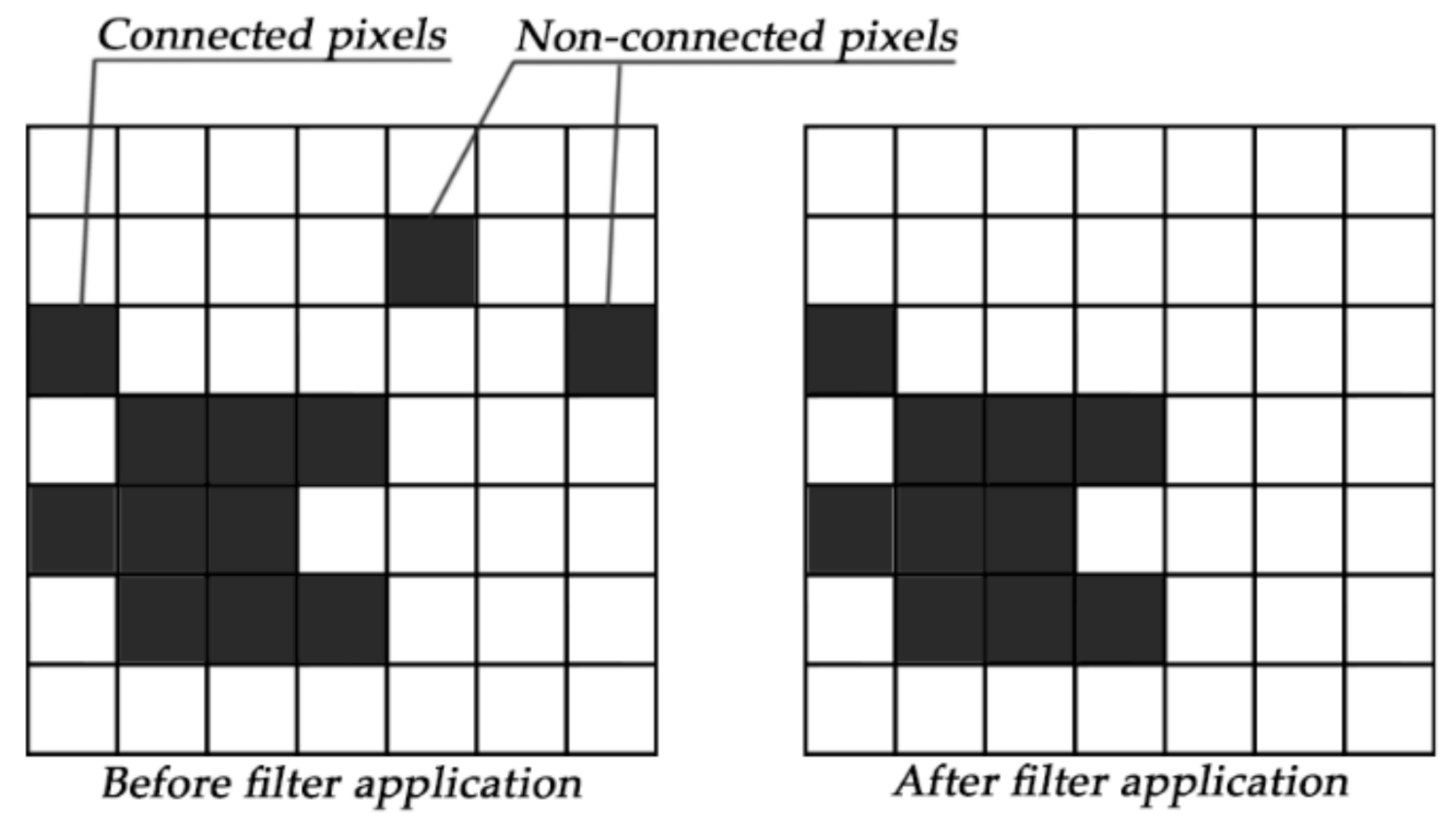
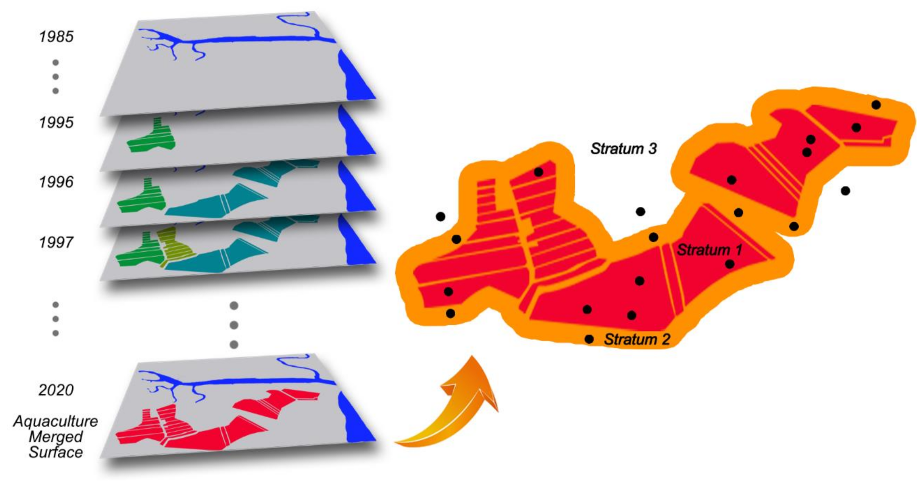
2.2. Data Processing

Data processing and analysis occurred inside a cloud computing environment, a setup combining the Google Earth Engine platform (GEE) and Tensor Flow library (Figure 2). All raster data and its sub-products are derived from the United States Geological Survey (USGS) Landsat Collection 1 Tier 1 Top of Atmosphere (TOA) data, which includes Level-1 Precision Terrain (L1TP) data [35,36,37].
For each year, Landsat Collection 1, Tier 1, TOA data was used to produce annual cloud-free composites, ranging from 1 January to 31 December. The cloud/shadow removal script takes advantage of the quality assessment (QA) band and the GEE median reducer. When used, QA values can improve data integrity by indicating which pixels might be affected by artifacts or subject to cloud contamination [38]. In conjunction, GEE can be instructed to pick the median pixel value in a stack of images. By doing so, the engine rejects values that are too bright (e.g., clouds) or too dark (e.g., shadows) and picks the median pixel value in each band over time.
Subsequently, the annual mosaics were sub-set to the area that comprises the BCZ to include areas where coastal aquaculture and saline ponds are more likely to occur (e.g., low-lying coastal and intertidal regions) and to exclude large areas where such characteristics are not expected to occur (e.g., highlands distant from the coastal plain and open ocean areas).
Next, the Modified Normalized Difference Water Index (MNDWI) [39] is computed to each of the annual mosaics, and over each, a K-means cluster analysis is executed. The K-means analysis helps create a binary water mask, labeling the pixels as water or non-water classes. Guided by the water/non-water mask’s existence, the coastal ponds of aqua or salt-culture features are visually delineated. This first visual delineation generates aqua-salt culture and non-aqua-salt culture samples. It is essential to highlight that no differentiation is made between coastal aquaculture or saline ponds; both elements are grouped as “aqua-salt culture” class members. Therefore, from this point on, every time aquaculture and salt-culture samples or classes are mentioned, it refers to an aqua-salt culture pattern.
Once the sample acquisition is finished, the U-Net algorithm is run. The classifier used three distinct spectral indices as input, the MNDWI [39], the Normalized Difference Vegetation Index-NDVI [40] and the Normalized Difference Soil Index-NDSI [41], resulting in the pre-filtered classification product. Our U-Net implementation followed its original conception [20], without extra tuning any of the hyperparameters available. Once convergence was reached and the classification was done, the classified data were injected back into GEE, where spatial-temporal filters and visual inspection occur. This phase was undertaken to correct misclassified data and evaluate the necessity of acquiring (or not) more training samples. Table 1 shows the classifier parameters.
Due to the U-Net pixel-wise output nature and the very long temporal series (35 years), a chain of post-classification filters was implemented. The chain starts by filling in possible no-data values. In a long-time series of severely cloud-affected regions, such as tropical coastal zones, it is expected that no-data values may populate some of the resultant median composite pixels. In this filter, no-data values (“gaps”) are theoretically not allowed and are replaced by the temporally nearest valid classification. If no “future” valid position is available in this procedure, then the no-data value is replaced by its previous valid class. To fill persistent no-data positions, up to three previous years can be used. Therefore, gaps should only exist if a given pixel has been permanently classified as no-data throughout the entire temporal domain. As shown in Figure 3, a mask of years was designed to keep track of the pixels’ temporal origin.
After gap filling, a temporal filter was executed. The temporal filter uses sequential classifications in a 3-year unidirectional moving window to identify temporally non-permitted transitions. Based on a single generic rule (GR), the temporal filter inspects the central position of three consecutive years (“ternary”), and if the extremities of the ternary are identical but the center position is not, then the central pixel is reclassified to match its temporal neighbor class, as shown in Table 2.
Later, a spatial filter was applied. To avoid unwanted modifications to the edges of the pixel groups (blobs), a spatial filter was built based on the “connectedPixelCount” function. Native to the GEE platform, this function locates connected components (neighbors) that share the same pixel value. Thus, only pixels that do not share connections to a predefined number of identical neighbors are considered isolated, as shown in Figure 4. In this filter, at least ten connected pixels are needed to reach the minimum connection value. Consequently, the minimum mapping unit is directly affected by the spatial filter applied, and it was defined as 10 pixels (~1 ha).
The accuracy assessment analysis was performed based on 900 independent samples taken at the Landsat pixel level for a pair of years, 1985 and 2019. A total of 1800 samples were used, 900 per year. These samples were generated by a stratified random sampling, where the aqua-salt culture class’s rareness compared to the non-aqua-salt culture class was taken into account. The validation samples’ distribution occurred in three different strata: (1) inside a temporally unified aqua-salt-culture surface (the annual classifications were merged, forming a single aqua-salt-culture surface) 450 samples were taken. (2) The previously merged stratum was buffered and 400 samples were taken inside the buffered zone, and (3) outside of the strata 1 and 2 boundaries, 50 samples were acquired. The total sample size was calculated according to the equation below.
n = N z γ 2 p 1 p N 1 e 2 + z γ 2 p 1 p
  • where;
  • n , is the sample size.
  • N , is the population size.
  • z , is the score of the normal distribution at a given confidence degree.
  • γ , is the confidence degree.
  • p , is the population proportion to be estimated.
  • e , the maximum error margin.
The validation samples were distributed to allow the possibility of evaluating the occurrence of both false positives and false negatives (Figure 5). A confidence interval of 95% and a maximum standard error of 5% were assumed to establish the sample size for each stratum, following the guidance of classical accuracy assessment practices [42,43,44].
The accuracy assessment of the 1985 and 2019 classification was calculated based on an independent visual inspection. This visual evaluation inspected the same Landsat annual mosaics given as input to the U-Net classifier. As decisive support data, the interpreters were also guided by Landsat multitemporal information, water indices, and high-resolution imagery available in Google Earth Pro.
Finally, an error matrix was produced for each of the inspected years. The following accuracy metrics were calculated per class, per year: Overall accuracy (OA), quantity and allocation disagreement (QD and AD), user and producer accuracy (CA and PA), omission and commission error (OE and CE), and the Kappa Coefficient (KC) [42,43,44].

3. Results

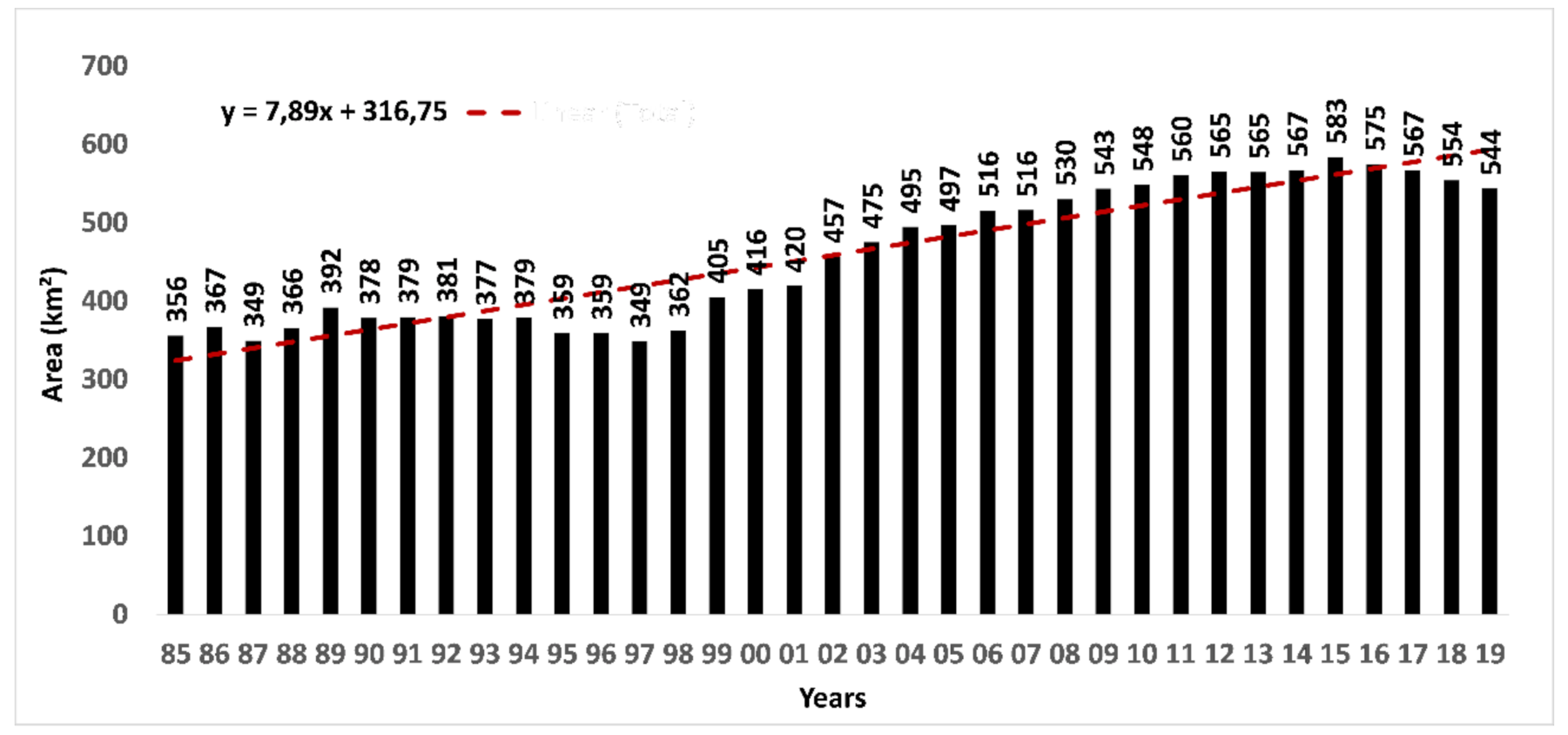
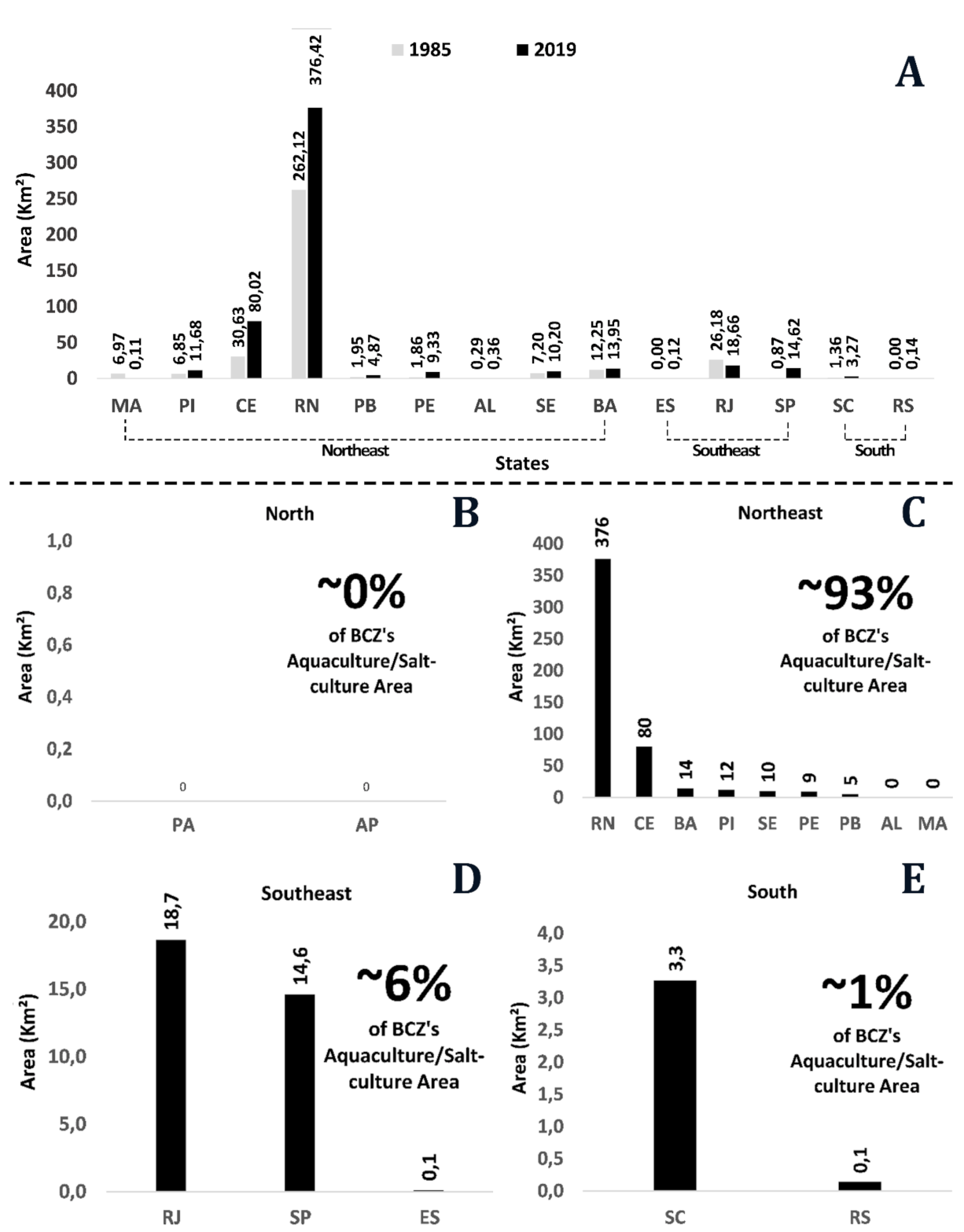
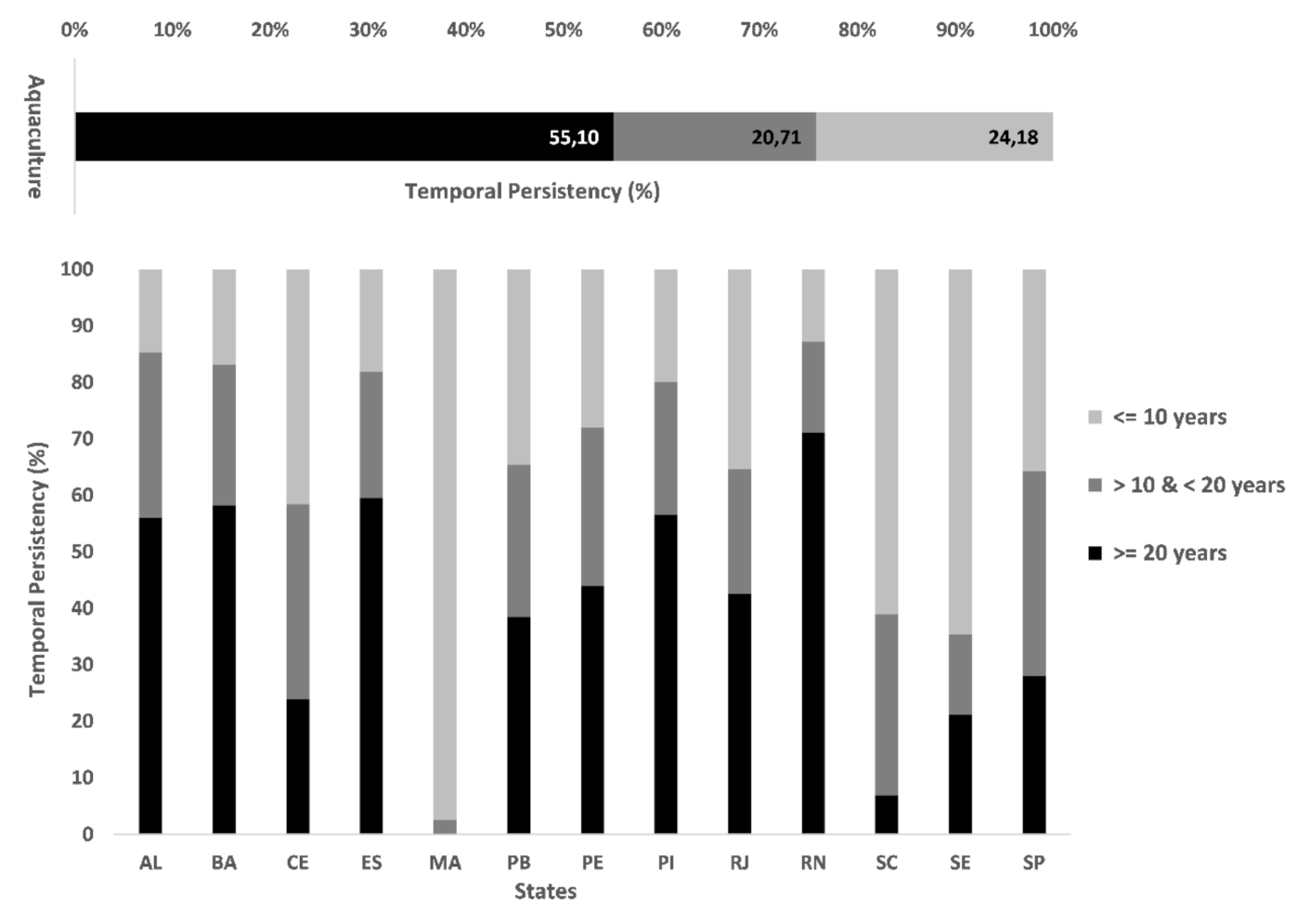
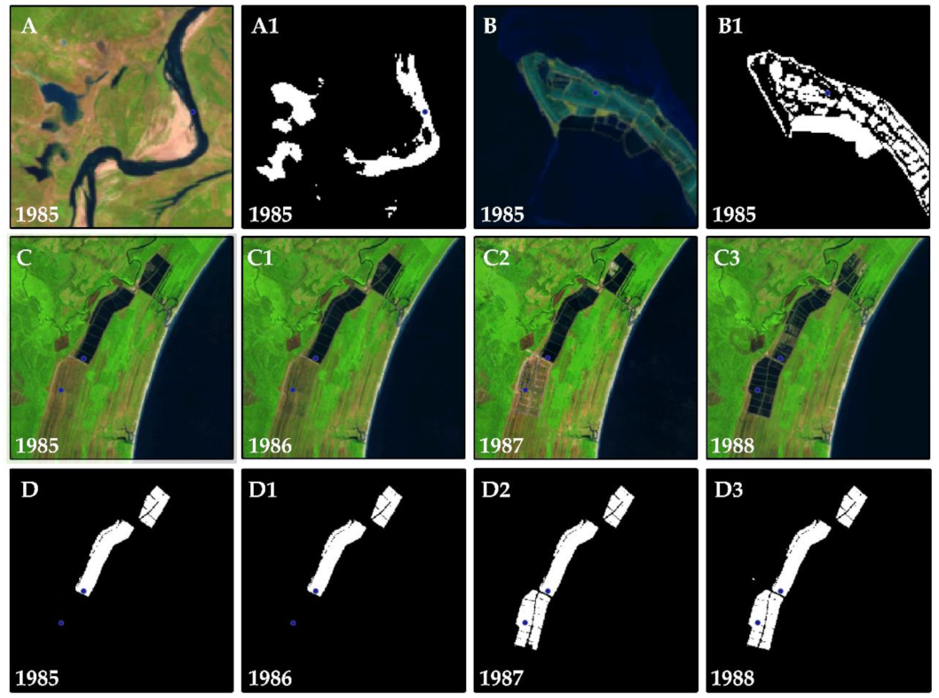
3.1. Spatio-Temporal Changes of Aqua-Salt Culture Ponds In BCZ

The coastal aqua-salt-culture activity has been identified and quantified for the entire BCZ over 34 years in a pioneering spatial and temporal coastal analysis. The aqua-salt-culture features were systematically and exhaustively mapped, producing digital spatial products and annual statistics ranging from 1985 to 2019 (Figure 6).
In Brazil, aqua-salt-culture ponds occupied ~356 km2 in 1985 and ~544 km2 in 2019, representing an area expansion of ~188 km2, ~52%. We can observe two distinct periods: from 85 to 98, certain stability is noticed, whereas from 1999 to 2019, a period of rapid growth appears. Considering the entire time-span, the area associated with aqua-salt-culture activity expanded 1.5× in 34 years (Figure 6). The late 1990s marked an accelerated development of aqua or salt-culture-related patterns. From 1997 to 2015, the area associated with this activity grew by a factor of ~1.7, jumping from 349 km2 to 583 km2, a 67% rise.
Regarding the presence or absence of aqua-salt-culture activity, out of 17 possible coastal states (Figure 1), three did not present any signal of aquaculture or saline-related patterns: Amapá (AP), Para (PA), and Parana (PR). The state of Maranhão (MA) presented the slightest, but not null, detected area. In MA, the detected ponds existed more prominently in the 1980s, but the signals of aquaculture or saline activities continuously decreased through time, reaching ~0.11 km2 in 2019 (Figure 7A).
In terms of coastal distribution, Figure 7A, the states of Rio Grande do Norte and Ceará present the most extensive aqua-salt-culture areas in the country, reaching ~376 km2 (~70%) and ~ 82 km2 (~15%) of aqua-salt-culture extension in Brazil, respectively, in 2019. Together, these two states represent ~85% of Brazil’s aqua-salt-culture land use.
Most Brazilian coastal states revealed an expansion of aqua-salt-culture land use in at least one of the compared years, 1985 and 2019 (Figure 7A). Interestingly, the states of AP, PA, and MA in the Northern sector, despite presenting extensive coastal zones and suitable conditions for developing various aquaculture products, especially shrimp culture, show no relevant sign of aqua-salt-culture infrastructure.
On a regional scenario, the South sectors represent approximately 1% of the total aqua-salt-culture area, none of that on the North coast (Figure 7B). In contrast, the Northeast sector concentrates 93% of the coastal aqua-salt-culture ponds (Figure 7C). The Southeast region is the second most relevant sector in terms of extension, contemplating 6% of the national coastal aqua-salt culture (Figure 7D). In comparison, the South sector contains only 1% of this land use area (Figure 7E).
From the perspective of temporal aquaculture persistence, ~55% of such coastal land-use remained unchanged for two decades or more, ~20% persisted between one and two decades, and ~24% remained stable for ten or fewer years, Figure 8, top bar. In this scenario, the state of Maranhão showed the lowest temporal persistence level; near 97% of its aqua-salt-culture ponds existed for less than ten years. In opposition, Rio Grande do Norte demonstrated the highest temporal ponds stability, with 71% of its aqua-salt-culture patterns remained unchanged for 20 years or more, as illustrated in Figure 8.

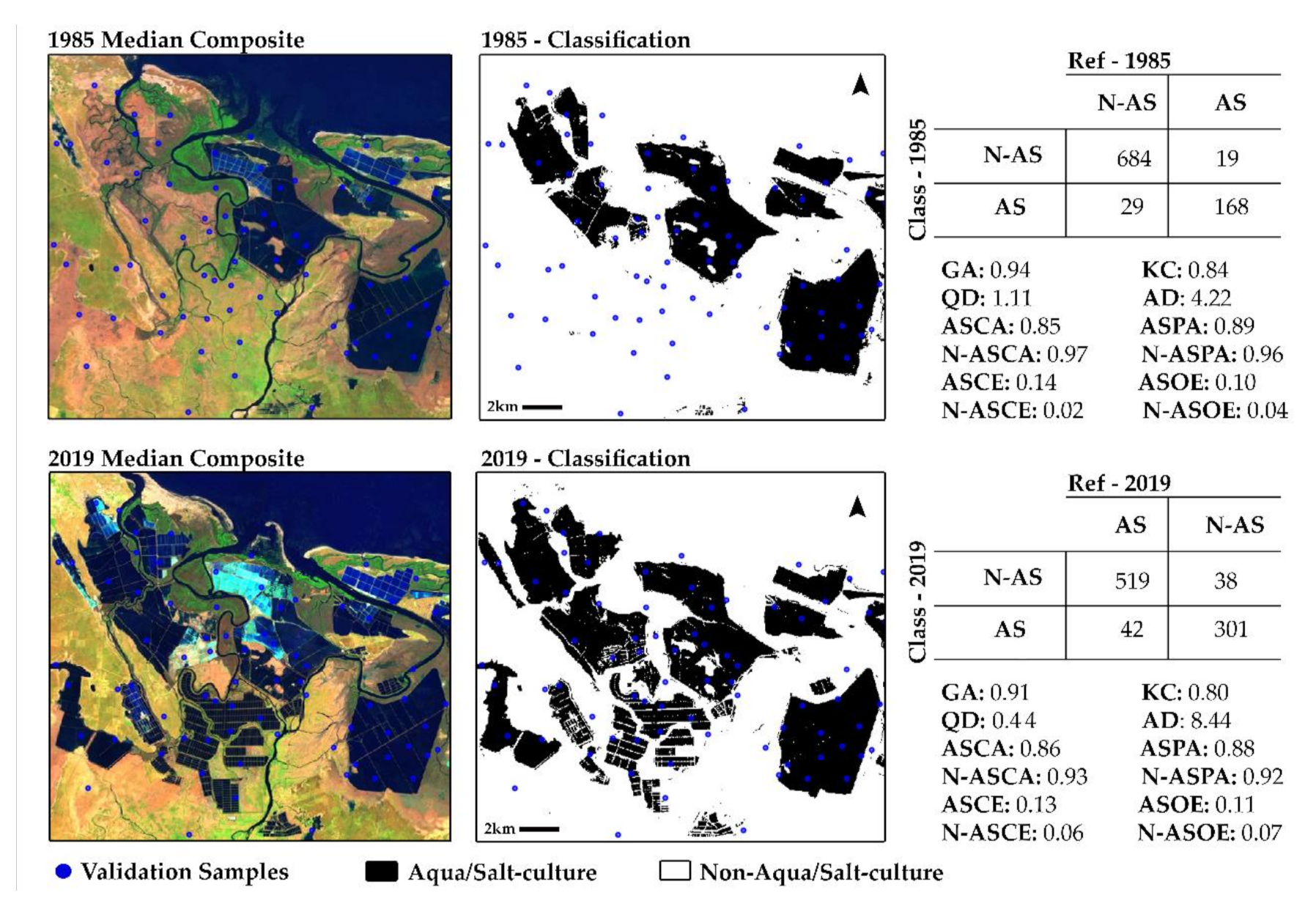
3.2. Aqua-Salt Culture Accuracy Assessment

The coastal spatial distribution of aqua-salt-culture ponds was unknown until this publication. Thus, along the BCZ a visual accuracy assessment campaign was executed to determine U-Net classified products’ agreement levels compared to a human-interpreted reference. Details related to the accuracy assessment sampling method are available in Figure 5. The accuracy campaign involved the cross-comparison of two sets of data, 1985 cloud-free composite (~400 Landsat scenes were available for this median composite) and the 2019 cloud-free composite (~1000 Landsat scenes constituted this composite). Figure 9 below shows the contingency tables for both years.
Compared to the 1985 reference, the classification developed herein achieves an overall agreement of 94% (OA = 0.94), quantity disagreement (QD), and allocation disagreement (AD) of 1.11% and 4.22%, respectively, a Kappa Coefficient (KC) ~0.84, and presents a low proportion of false negatives (~0.10). It shows around 14% of false positives, representing roughly 1/6 of disagreement between what is referred to as N-AS, but is classified as AS (commission error).
Regarding 2019 data, the degree of global concordance is equally high, achieving an overall agreement of 91% (OA = 0.91). The QD and AD were 0.44% and 8.44%, respectively, with KC ~0.81. The presented proportions of aqua-salt culture’s false positives and false negatives were smaller than 15%, with AS commission errors (ASCE) ~0.13, while AS omission errors (ASOE) reached ~0.11. The N-AS class had omission and commission errors minor than 7% (N-ASCE ~0.06 and ASOE ~0.07).

4. Discussion

For the first time in the scientific literature, the Brazilian coastal aqua and salt-culture ponds were systematically and exhaustively mapped. Studies of such nature provide a better understanding of the country’s coastal dynamics, allowing an annual analysis of two of the most classical coastal land-uses, directly subsidizing national and regional policymakers.
In the last three decades, two distinct moments can be highlighted in Brazil’s coastal aqua-salt-culture occupation (Figure 6). From 1985 to 1998, a moment of stability was noticed, in which variations of nearly ±5% alternately occur. On the other hand, from 1999 to 2019, a moment of rapid growth marked an accelerated expansion of the activity. This spatial-temporal behavior matches the history of marine salt production in Brazil [45,46,47], particularly in the states of RN and CE, responsible for ~85% of Brazil’s aqua-salt-culture area in 2019 (Figure 7).
The discrepant spatial distribution of the aqua-salt pond areas in the BCZ is primarily related to geological and economic characteristics more than any other. Most of the national saline industry was purposely implanted in areas where salt formation through solar evaporation naturally occurs (hypersaline-shallow plains over dry climate) [4,32]. Moreover, physically dependent on solar efficiency, evaporation ponds tend to be much larger and shallower than aquaculture ones. Together, this set of characteristics helps comprehend the spatial distortions involving RN and CE compared to the remaining coastal states.
Similarly, economic, geological, and climatic characteristics might be the most significant factors influencing the absence of relevant areas of salines or aquaculture in the North of Brazil. Amapá, Pará, and Maranhão’s states present extensive coastal plains and suitable conditions for developing various aqua-salt-culture products. However, all three states lack economic competitiveness due to the absence of requisite infrastructure to sustain large-scale aquaculture farming [31] and accentuated precipitation regimes compromise marine salt-production [45,47,48,49]. Furthermore, the densest and well-developed mangrove vegetation in the country acts as a natural barrier, challenging the implementation of artificial ponds over the dense mangrove forest [8,21,24,50].
Regarding the concordance levels, when cross-compared to the references of 1985 and 2019, the U-net classified product achieved high levels of overall agreement and kappa coefficients, OA > 90% and KC > 0.80 for both years and a small proportion of quantity and allocation disagreements. The worst QD measure case reached ~1% for 1985 data, and the max AD measure was not higher than 9%; AD ~8.5% in 2019. Moreover, both datasets presented relatively low AS commission and omission errors. The omissions levels reached ~10%, while commissions were ~14%, Figure 7.
The inspected commission and omission errors were mainly associated with two types of incongruences; (1) U-Net Errors (UE): for the U-Net classifier, the context domain is given by the joint use of spectral and spatial information. Thus, lack of training data may fail to successfully transfer/learn the contextual knowledge necessary to decide upon aquaculture or non-aquaculture. (2) Filtering Errors (FE): aquaculture and saline ponds may suffer from fluctuations in their water levels. Still, even without water for a short amount of time, the land use related to an empty artificial pond cannot be classified as non-aquaculture. Although combined with UE, an inaccurate classification may be propagated through time due to the temporal-filter algorithm’s action (Figure 10).
Figure 10 shows the two most representative types of misclassifications. The pair-wise A-A1 and B-B1 demonstrate an inaccurate aqua-salt-culture label due to TEs. In A-A1, a portion of a river and natural lagoons were wrongly associated with the aqua-salt culture class. In B-B1, TEs resulted in partially accurate classification. Inner parts of the aqua-salt-culture-dominated cuspate spit were classified as non-aquaculture. In the C sequence, the water presence/absence is evident through time. In D, the temporal filter acts and uses temporal information to classify empty artificial ponds as aquaculture/salt-culture. Although the temporal rule’s simplicity may need to be revisited, seeing that once helping to stabilize the expected water fluctuation, the temporal filter may also propagate errors through time.
Thus, despite the overall data agreement and its relatively low commission and omission metrics, there is still room for improvements in the data accuracy levels. In this sense, capturing a more diverse group of training samples in terms of spectral and geometrical variability, increasing the sample’s representativity throughout the temporal series, and revisiting the post-classification algorithms are essential strategies to be further implemented.
It is of fundamental importance to mention that time is one of the most significant economic constraints related to cloud services use as an alternative to address large-scale project necessities. To date, there is no cloud processing service, which allows the consumption of enormous processing power over large volumes of data, and many hours of machine use, in an absolute free of charge manner. There will always be a charge in all commercially available alternatives on one or more of these characteristics.
Backed by a computer engine of 32 GB of RAM and Nvidia GPUs, our pipeline processed an extension of ~65 Landsat path and rows, over 33 years of data, covering the entire BCZ, representing 2000+ processed Landsat scenes. In this scenario, the time consumption related to testing/training and prediction time reached approximately 192 h (~8 days of cloud usage).
The following steps of this research consist of (a) improving the post-classification mechanism to identify empty artificial ponds more accurately, (b) expanding the analysis to the entire continental region of the country (including the aqua or salt-culture that may exist further inland), and (c) using refined spatial resolution data. Considering the importance of the contextual domain, the better the data’s spatial resolution is, the better it is for context recognition. Thus, our future works will incorporate Landsat panchromatic data and the 10 m resolution Sentinel-2A full dataset.

5. Conclusions

Studies of this nature fill up a relevant information gap, exhaustively mapping the entire BCZ and distinguishing its aqua-salt-culture spatial distribution. Using a massive, publicly available, remotely sensed time series, this study contributes to the multi-scale understanding of aquacultures and salt-culture occupation across the BCZ, which provides a better understanding of Brazil’s coastal dynamics, directly subsidizing national and regional policymakers.
This work’s findings pave the path towards understanding the direct and indirect influences that aquaculture and marine salt production might have on the coastal environment’s sustainability. The developed pipeline seems reasonably scalable, sufficiently generic, and suitable for large-scale aquaculture/saline automatic identification.
The method allowed a systematic and continuous delineation of aquaculture and saline patterns, supporting digital cartographic products and annual statistics, ranging from 1985 to 2019. The data specialized and quantified the contribution of each one of ZCB’s states. Out of 17 possible coastal states, three did not present any signal of aqua-salt-culture-related patterns (AP, PA, and PR). The state of Maranhão (MA) presented the smallest detected area, where signs of aquaculture or saline ponds were more prominent in the 1980s.
Further developments may allow its applicability to larger continental areas, such as the entire country, including continental aqua-salt culture or even South America in its entirety, and incorporate Landsat panchromatic data as well as the Sentinel-2 10 m dataset.
All the data produced are available through the website http://www.solved.eco.br/datasets/ (accessed on 4 April 2021) and will be transferred to the MapBiomas project (www.mapbiomas.org) (accessed on 4 April 2021) in MapBiomas Collection 6.0. All the codes used in this work are available through the GitHub https://github.com/solvedecobr/aqua-salt-net (accessed on 4 April 2021).

Author Contributions

Conceptualization, C.D. and L.C.; Data curation, C.D., L.C. and P.W.M.S.-F.; Formal analysis, C.D.; Funding acquisition, P.W.M.S.-F.; Investigation, C.D.; Methodology, C.D., L.C. and M.L.P.; Project administration, P.W.M.S.-F.; Supervision, P.W.M.S.-F.; Validation, L.S., A.F.F., L.R.F.B. and M.A.; Visualization, L.S.; Writing—original draft, C.D.; Writing—review and editing, C.D., M.A. and P.W.M.S.-F. All authors have read and agreed to the final version of the manuscript.

Funding

This research was funded by the Brazilian National Council for Scientific and Technological Development (CNPq): 870005/1997-9, 310283/2019-1, 306334/2020-8 and the MapBiomas Project. The processing charges were covered by the Instituto Tecnológico Vale, as part of the project “Environmental Studies in the São Marcos Bay, Amazonia, Brazil”. Research grant: RBRS000603.95.

Data Availability Statement

All the data produced are available through the website http://www.solved.eco.br/datasets/ and will be transferred to the MapBiomas project (www.mapbiomas.org) in MapBiomas Collection 6.0. All the codes used in this work are available through the GitHub https://github.com/solvedecobr/aqua-salt-net.

Acknowledgments

The authors are grateful to Tasso Azevedo, general coordinator of the MapBiomas Project and the SEEG initiative. Lastly, the authors acknowledge the Brazilian National Council for Scientific and Technological Development (CNPq) for the financial support received during this research and the Instituto Tecnológico Vale, for covering all the publication fees.

Conflicts of Interest

The authors declare no conflict of interest.

References

  1. Food And Agriculture Organization (FAO). Fishery and Aquaculture Statistics—2017; FAO: Rome, Italy, 2019; ISBN 9789251316696. [Google Scholar]
  2. Food And Agriculture Organization (FAO). The State of World Fisheries and Aquaculture 2018—Meeting the Sustainable Development Goals; FAO: Rome, Italy, 2018; ISBN 9789251305621. [Google Scholar]
  3. Food And Agriculture Organization (FAO). The State of World Fisheries and Aquaculture 2020; FAO: Rome, Italy, 2020. [Google Scholar]
  4. Ottinger, M.; Clauss, K.; Kuenzer, C. Aquaculture: Relevance, distribution, impacts and spatial assessments—A review. Ocean Coast. Manag. 2016, 119, 244–266. [Google Scholar] [CrossRef]
  5. Giri, C.; Ochieng, E.; Tieszen, L.L.; Zhu, Z.; Singh, A.; Loveland, T.; Masek, J.; Duke, N. Status and distribution of mangrove forests of the world using earth observation satellite data. Glob. Ecol. Biogeogr. 2011, 20, 154–159. [Google Scholar] [CrossRef]
  6. Thomas, N.; Bunting, P.; Lucas, R.; Hardy, A.; Rosenqvist, A.; Fatoyinbo, T. Mapping Mangrove Extent and Change: A Globally Applicable Approach. Remote Sens. 2018, 10, 1466. [Google Scholar] [CrossRef] [Green Version]
  7. Bunting, P.; Rosenqvist, A.; Lucas, R.M.; Rebelo, L.M.; Hilarides, L.; Thomas, N.; Hardy, A.; Itoh, T.; Shimada, M.; Finlayson, C.M. The global mangrove watch—A new 2010 global baseline of mangrove extent. Remote Sens. 2018, 10, 1669. [Google Scholar] [CrossRef] [Green Version]
  8. Diniz, C.; Cortinhas, L.; Nerino, G.; Rodrigues, J.; Sadeck, L.; Adami, M.; Souza-Filho, W.P. Brazilian Mangrove Status: Three Decades of Satellite Data Analysis. Remote Sens. 2019, 11, 808. [Google Scholar] [CrossRef] [Green Version]
  9. Pekel, J.-F.; Cottam, A.; Gorelick, N.; Belward, A.S. High-resolution mapping of global surface water and its long-term changes. Nature 2016, 540, 418–422. [Google Scholar] [CrossRef]
  10. Luijendijk, A.; Hagenaars, G.; Ranasinghe, R.; Baart, F.; Donchyts, G.; Aarninkhof, S. The State of the World’s Beaches. Sci. Rep. 2018, 8, 6641. [Google Scholar] [CrossRef]
  11. Worthington, T.A.; zu Ermgassen, P.S.E.; Friess, D.A.; Krauss, K.W.; Lovelock, C.E.; Thorley, J.; Tingey, R.; Woodroffe, C.D.; Bunting, P.; Cormier, N.; et al. A global biophysical typology of mangroves and its relevance for ecosystem structure and deforestation. Sci. Rep. 2020, 10, 14652. [Google Scholar] [CrossRef]
  12. Lagomasino, D.; Fatoyinbo, T.; Lee, S.; Feliciano, E.; Trettin, C.; Simard, M. A Comparison of Mangrove Canopy Height Using Multiple Independent Measurements from Land, Air, and Space. Remote Sens. 2016, 8, 327. [Google Scholar] [CrossRef] [Green Version]
  13. Lagomasino, D.; Fatoyinbo, T.; Lee, S.; Feliciano, E.; Trettin, C.; Shapiro, A.; Mangora, M.M. Measuring mangrove carbon loss and gain in deltas. Environ. Res. Lett. 2019, 14, 25002. [Google Scholar] [CrossRef]
  14. Duan, Y.; Li, X.; Zhang, L.; Chen, D.; Liu, S.; Ji, H. Mapping national-scale aquaculture ponds based on the Google Earth Engine in the Chinese coastal zone. Aquaculture 2020, 520, 734666. [Google Scholar] [CrossRef]
  15. Xia, Z.; Guo, X.; Chen, R. Automatic extraction of aquaculture ponds based on Google Earth Engine. Ocean Coast. Manag. 2020, 198, 105348. [Google Scholar] [CrossRef]
  16. Marinho, R.R.; Filizola Junior, N.P.; Cremon, É.H. Analysis of Suspended Sediment in the Anavilhanas Archipelago, Rio Negro, Amazon Basin. Water 2020, 12, 1073. [Google Scholar] [CrossRef] [Green Version]
  17. Marinho, R.R.; Harmel, T.; Martinez, J.-M.; Filizola Junior, N.P. Spatiotemporal Dynamics of Suspended Sediments in the Negro River, Amazon Basin, from In Situ and Sentinel-2 Remote Sensing Data. ISPRS Int. J. Geo Inf. 2021, 10, 86. [Google Scholar] [CrossRef]
  18. Mertes, L.A.K.; Smith, M.O.; Adams, J.B. Estimating suspended sediment concentrations in surface waters of the Amazon River wetlands from Landsat images. Remote Sens. Environ. 1993, 43, 281–301. [Google Scholar] [CrossRef]
  19. Lobo, F.; Souza-Filho, P.; Novo, E.; Carlos, F.; Barbosa, C. Mapping Mining Areas in the Brazilian Amazon Using MSI/Sentinel-2 Imagery (2017). Remote Sens. 2018, 10, 1178. [Google Scholar] [CrossRef] [Green Version]
  20. Ronneberger, O.; Fischer, P.; Brox, T. U-Net: Convolutional Networks for Biomedical Image Segmentation. CoRR 2015, 9351, 234–241. [Google Scholar]
  21. Schaeffer-Novelli, Y.; Cintrón-Molero, G.; Adaime, R.R.; de Camargo, T.M.; Cintron-Molero, G.; de Camargo, T.M. Variability of Mangrove Ecosystems along the Brazilian Coast. Estuaries 1990, 13, 204–218. [Google Scholar] [CrossRef]
  22. Rodrigues, S.W.P.; Souza-Filho, P.W.M. Use of Multi-Sensor Data to Identify and Map Tropical Coastal Wetlands in the Amazon of Northern Brazil. Wetlands 2011, 31, 11–23. [Google Scholar] [CrossRef]
  23. Souza Filho, P.W.M. Costa de manguezais de macromaré da Amazônia: Cenários morfológicos, mapeamento e quantificação de áreas usando dados de sensores remotos. Rev. Bras. Geofísica 2005, 23, 427–435. [Google Scholar] [CrossRef] [Green Version]
  24. Nascimento, W.R., Jr.; Souza-Filho, P.W.M.; Proisy, C.; Lucas, R.M.; Rosenqvist, A. Mapping changes in the largest continuous Amazonian mangrove belt using object-based classification of multisensor satellite imagery. Estuar. Coast. Shelf Sci. 2013, 117, 83–93. [Google Scholar] [CrossRef]
  25. Dominguez, J.M.L. The Coastal Zone of Brazil. In Geology and Geomorphology of Holocene Coastal Barriers of Brazil; Springer: Berlin/Heidelberg, Germany, 2009; pp. 17–51. ISBN 978-3-540-44771-9. [Google Scholar]
  26. IBGE. Sistema IBGE de Recuperação Automática (SIDRA)—Produção da Aquicultura Brasileira; Instituto Brasileiro de Geografia e Estatística: Brasília, Brazil, 2019. [Google Scholar]
  27. Pereira, J.M.P.; de Souza, E.N.V.; Candido, J.R.B.; Dantas, M.D.A.; Nunes, A.R.D.; Ribeiro, K.; Teixeira, D.I.A.; Lanza, D.C.F. Alternative PCR primers for genotyping of Brazilian WSSV isolates. J. Invertebr. Pathol. 2019, 162, 55–63. [Google Scholar] [CrossRef] [PubMed]
  28. de Bandeira, J.T.; de Morais, R.S.M.M.; e Silva, R.P.P.; Mendes, E.S.; da Silva, S.M.B.C.; dos Santos, F.L. First report of white spot syndrome virus in wild crustaceans and mollusks in the Paraíba River, Brazil. Aquac. Res. 2019, 50, 680–684. [Google Scholar] [CrossRef]
  29. Santos, R.N.; Varela, A.P.M.; Cibulski, S.P.; Esmaile, S.; Lima, F.; Rosado Spilki, F.; Schemes Heinzelmann, L.; Bordin da Luz, R.; Abreu, P.C.; Roehe, P.M.; et al. A Brief History of White spot syndrome virus and Its Epidemiology in Brazil. Virus Rev. Res. 2013, 18, 1–5. [Google Scholar] [CrossRef] [Green Version]
  30. Roubach, R.; Correia, E.S.; Zaiden, S.; Martino, R.C.; Cavalli, R.O. Aquaculture in Brazil. World Aquac. Rouge 2003, 34, 28–35. [Google Scholar]
  31. Tenório, G.S.; Souza-Filho, P.W.M.; Ramos, E.M.L.S.; Alves, P.J.O. Mangrove shrimp farm mapping and productivity on the Brazilian Amazon coast: Environmental and economic reasons for coastal conservation. Ocean Coast. Manag. 2015, 104, 65–77. [Google Scholar] [CrossRef]
  32. de Rocha, I.P. Shrimp farming in Brazil: Burgeoning industry recovering, future holds potential. In Global Aquaculture Alliance; Abccam: Recife, Brazil, 2010; pp. 43–45. [Google Scholar]
  33. Bueno, G.W.; Ostrensky, A.; Canzi, C.; de Matos, F.T.; Roubach, R. Implementation of aquaculture parks in Federal Government waters in Brazil. Rev. Aquac. 2015, 7, 1–12. [Google Scholar] [CrossRef]
  34. Lima, L.B.; Oliveira, F.J.M.; Giacomini, H.C.; Lima-Junior, D.P. Expansion of aquaculture parks and the increasing risk of non-native species invasions in Brazil. Rev. Aquac. 2018, 10, 111–122. [Google Scholar] [CrossRef]
  35. USGS. Landsat 8 (L8) Data Users Handbook; EROS: Sioux Falls, SD, USA, 2015. [Google Scholar]
  36. Storey, J.; Choate, M.; Lee, K. Landsat 8 Operational Land Imager On-Orbit Geometric Calibration and Performance. Remote Sens. 2014, 6, 11127–11152. [Google Scholar] [CrossRef] [Green Version]
  37. Teillet, P.M.; Barker, J.L.; Markham, B.L.; Irish, R.R.; Fedosejevs, G.; Storey, J.C. Radiometric cross-calibration of the Landsat-7 ETM+ and Landsat-5 TM sensors based on tandem data sets. Remote Sens. Environ. 2001, 78, 39–54. [Google Scholar] [CrossRef] [Green Version]
  38. USGS. Landsat Collection 1 Level 1 Product Definition; EROS: Sioux Falls, SD, USA, 2017; p. 26. [Google Scholar]
  39. Xu, H. Modification of normalised difference water index (NDWI) to enhance open water features in remotely sensed imagery. Int. J. Remote Sens. 2006, 27, 3025–3033. [Google Scholar] [CrossRef]
  40. Tucker, C.J. Red and photographic infrared linear combinations for monitoring vegetation. Remote Sens. Environ. 1979, 8, 127–150. [Google Scholar] [CrossRef] [Green Version]
  41. Rogers, A.S.; Kearney, M.S. Reducing signature variability in unmixing coastal marsh Thematic Mapper scenes using spectral indices. Int. J. Remote Sens. 2004, 25, 2317–2335. [Google Scholar] [CrossRef]
  42. Olofsson, P.; Foody, G.M.; Herold, M.; Stehman, S.V.; Woodcock, C.E.; Wulder, M.A. Good practices for estimating area and assessing accuracy of land change. Remote Sens. Environ. 2014, 148, 42–57. [Google Scholar] [CrossRef]
  43. Pontius, R.G.; Santacruz, A. Quantity, exchange, and shift components of difference in a square contingency table. Int. J. Remote Sens. 2014, 35, 7543–7554. [Google Scholar] [CrossRef]
  44. Stehman, S.V. Estimating area and map accuracy for stratified random sampling when the strata are different from the map classes. Int. J. Remote Sens. 2014, 35, 4923–4939. [Google Scholar] [CrossRef]
  45. Diniz, M.T.M.; Vasconcelos, F.P.; Diniz, M.T.M.; Vasconcelos, F.P. Natural conditions for the sea salt production in Brazil. Mercator 2017, 16, 1–19. [Google Scholar] [CrossRef]
  46. Costa, D.F.d.S.; da Silva, A.A.; Medeiros, D.H.M.; Lucena Filho, M.A.; Rocha, R.D.M.; Lillebo, A.I.; Soares, A.M.V.M. Breve revisão sobre a evolução histórica da atividade salineira no estado do Rio Grande do Norte (Brasil). Soc. Nat. 2013, 25, 21–34. [Google Scholar] [CrossRef]
  47. Diniz, M.T.M.; Vasconcelos, F.P.; Martins, M.B. Inovação tecnológica na produção brasileira de sal marinho e as alterações sócioterritoriais dela decorrentes: Uma análise sob a ótica da Teoria do Empreendedorismo de Schumpeter. Soc. Nat. 2015, 27, 421–437. [Google Scholar] [CrossRef] [Green Version]
  48. Bhat, A.H.; Sharma, K.C.; Banday, U.J. Impact of Climatic Variability on Salt Production in Sambhar Lake, a Ramsar Wetland of Rajasthan, India. Middle East J. Sci. Res. 2015, 23, 2060–2065. [Google Scholar]
  49. Lima, K.C. Impactos Econômicos das Mudanças Climáticas sobre a Indústria de Sal Marinho na Principal Região Produtora do Brasil. Rev. Bras. Geogr. Física 2017, 10, 584–596. [Google Scholar] [CrossRef]
  50. ICMBio. Atlas dos Manguezais do Brasil, 1st ed.; ICMBio: Brasília, Brazil, 2017; ISBN 978-85-61842-75-8. [Google Scholar]
Figure 1. The Brazilian Coastal Zone (BCZ) was divided into four regional sectors; North, Northeast, Southeast, and South. The following acronyms represent the Brazilian coastal states: AL (Alagoas), AP (Amapá), BA (Bahia), CE (Ceará), ES (Espírito Santo), MA (Maranhão), PA (Pará), PB (Paraíba), PE (Pernambuco), PI (Piauí), PR (Paraná), RJ (Rio de Janeiro), RN (Rio Grande do Norte), SC (Santa Catarina), SE (Sergipe), and SP (São Paulo).
Remotesensing 13 01415 g001
Figure 2. Aquaculture Earth Engine-TensorFlow pipeline. The process is structured in 4 steps. First (1), GEE is used to generate the cloud-free composites and create the initial training dataset. Second (2), the mosaics and training data are stored inside the Google Cloud Storage. Three (3), the patch-wise training and classification are initiated. In the fourth step (4), the classified product is spatial and temporally filtered. The filtered product is visual and statistically inspected. Multiple iterations may be used until a satisfactory degree of spatial and temporal quality is achieved.
Remotesensing 13 01415 g002
Figure 3. Gap-filling mechanism. The next valid classification replaces existing no-data values. If no “future” valid position is available, then the no-data value is replaced by its previous valid classification, based on up to a maximum of three (3) prior years. To keep track of pixel temporal origins, a mask of years was built.
Remotesensing 13 01415 g003
Figure 4. The spatial filter removes pixels that do not share neighbors of identical value. The minimum connection value was 10 pixels.
Remotesensing 13 01415 g004
Figure 5. A total of 900 independent samples were taken at the Landsat pixel level in 1985 and 2019. 1800 samples in total. The sample distribution occurred in three different strata: (1) 450 samples inside a temporally merged aquaculture surface. (2) 400 samples inside the stratum 1 buffered zone, and (3) 50 samples outside of the strata 1 and 2 boundaries.
Remotesensing 13 01415 g005
Figure 6. Annual variation of aqua-salt-culture area, in km2, from 1985 to 2019. The area associated with this activity expanded 1.5× in 34 years—an increase of ~51%. The black bars denote the aqua-salt-culture area. The red dashed line indicates the ascendant trend of aqua-salt-culture evolution.
Remotesensing 13 01415 g006
Figure 7. (A) Brazil’s aqua-salt-culture area per federal unit in km2. Aqua-salt-culture extension in km2 and percentage per sector: (B) North, (C) Northeast, (D) Southeast, and (E) South are responsible, in sequence, by 0%, 93%, 6%, and 1% of the national aquaculture distribution.
Remotesensing 13 01415 g007
Figure 8. Aqua-salt-culture persistence at national and regional scales. The top horizontal bar shows the overall aqua-salt-culture persistence. The vertical bars show the aqua-salt-culture persistence per state. The x-axis represents the state distributions, while the y-axis represents the aqua/salt-culture cover temporal persistence percentages (%). Black represents 20 years or more of stability, and dark grey indicates stability between 10 and 20 years, and light grey represents stability for less than ten years.
Remotesensing 13 01415 g008
Figure 9. On the left are the 1985 and 2019 median composites. In the central portion, U-Net classifications from 1985 and 2019. The contingency tables (right) show the agreement levels between the reference and classified data. Values on the main diagonal are the numbers of concordant pixels. On the off-diagonal, those above are commission differences, and those below are omission differences. OA stands for overall agreement. QD and AD for Quantity and Allocation Disagreements, KC denotes the Kappa coefficient. ASCA/N-ASCA means Aqua-Salt-culture/Non-Aqua-Salt-culture Consumer Accuracy, while AS/N-AS refers to the Aquaculture/Non-Aquaculture Producers Accuracy. Both classes’ commission and omission errors are referred to as ASCE, N-ASCE, ASOE, N-ASOE.
Remotesensing 13 01415 g009
Figure 10. The two most representative types of misclassifications. Due to UEs, the pairs A-A1 and B-B1 indicate erroneous classification. A river segment and natural lagoons were incorrectly labeled in A-A1. In B-B1, inner parts of the aqua-salt culture dominated cuspate spit were classified as a non-aqua-salt culture. In the C and D sequences, the temporal filter operates and uses temporal information to classify empty artificial ponds as an aqua-salt culture. Although, while helping to stabilize the expected water fluctuation, the temporal filter may also propagate errors through time. Blue dots are accuracy assessment samples.
Remotesensing 13 01415 g010
Table 1. Classifier attributes and classification parameters. In total, three distinct attributes were used.
ParametersValues
ClassifierU-Net
Tile-Size256 × 256 pixels
OptimizerSGD
Learning Rate0.1
Momentum0.9
Decay1e−4
Samples8400 (geometries)
AttributesMNDWI, NDVI, and NDSI
Classes2 (Aqua-Salt-culture and Non-Aqua-Salt-culture)
Table 2. The temporal filter inspects the central position of three consecutive years, and in cases of identical extremities, the center position is reclassified to match its neighbor. T1, T2, and T3 stand for positions one (1), two (2), and three (3), respectively. GR means “generic rule”, while AS and N-AS represent aqua-salt-culture and non-aqua-salt culture pixels.
Rule Input (Year) Output
T1T2T3T1T2T3
GRASN-ASASASASAS
GRN-ASASN-ASN-ASN-ASN-AS
Publisher’s Note: MDPI stays neutral with regard to jurisdictional claims in published maps and institutional affiliations.

