Article

Analysis of Land Development Drivers Using Geographically Weighted Ridge Regression

by
Pariya Pourmohammadi
1,2,*,
Michael P. Strager
3,
Michael J. Dougherty
2 and
Donald A. Adjeroh
1
1
Lane Department of Computer Science and Electrical Engineering, Benjamin M. Statler College of Engineering and Mineral Resources, West Virginia University, Morgantown, WV 26506-6109, USA
2
School of Design and Community Development, Davis College of Agriculture, Natural Resources and Design, West Virginia University, Morgantown, WV 26506-6108, USA
3
School of Natural Resources, Davis College of Agriculture, Natural Resources and Design, West Virginia University, Morgantown, WV 26506-6108, USA
*
Author to whom correspondence should be addressed.
Remote Sens. 2021, 13(7), 1307; https://doi.org/10.3390/rs13071307
Submission received: 30 January 2021 / Revised: 1 March 2021 / Accepted: 16 March 2021 / Published: 30 March 2021

Abstract

:
Land development processes are driven by complex interactions between socio-economic and spatial factors. Acquiring an understanding of such processes and the underlying procedures helps urban and regional planners, environmental scientists, and policy makers to base their decisions on valid and profound information. In this work, remote-sensing-derived land-cover data were used to characterize the patterns of land development from the beginning of 1985 to the beginning of 2015, in the state of West Virginia (WV), US. We applied spatial pattern analysis, ridge regression, and Geographically Weighted Ridge Regression (GWRR) to examine the impact of population, energy resources, existing land developments dynamics, and economic status on land transformation. We showed that in presence of multicollinearity of explanatory variables, how penalizing regression models in both local and global levels lead to a better fit and decreases the model’s variance. We used geographical error analysis of regression models to visualize the difference between the model estimates and actual values. The findings of this research indicate that because of shifting geography of opportunities, the patterns and processes of land development in the studied region are unstable. This leads to fragmented land developments and prevents formation of large communities.

Graphical Abstract

1. Introduction

In areas with an abundance of natural resources, landscape changes result in immense costs and irrevocable consequences [1,2]. Investigation of drivers of landscape change is referred to as the study of the influential processes in the evolutionary trajectory of the landscape [3]. Such analysis is viable through study of the connections between people and their environment which helps in understanding the societal demands and economic situations of regions [3]. Study of land development and its different aspects is one of the applied methods for investigating the landscape change.
In this study the developed lands are defined as the lands wherein there are some constructed materials with more than 20% of impervious surface. This definition is from low/medium/high intensity developed land class of the Anderson Land Cover Classification System [4] used in National Land Cover Dataset (NLCD) 2016 [5]. Acquiring an insight into the drivers of developed land expansion trends helps decision makers to inspect the patterns and causes of these processes and make decisions for smart land management towards resilient communities, scenario modeling for disaster management, and predicting the future of land transformation [6]. To describe the overall data relationships, regression models, like Ordinary Least Squares (OLS), are widely applied. When those relationships are consistent across a study, the global regression model is applicable. However, if the explanatory variables exhibit non-stationary relationships (regional variation), global models tend to fall apart, unless robust methods are used to compute regression results [7,8]. Ideally, to capture the regional variation inherent in the dependent variables, there is a need to identify a full set of explanatory variables. If one cannot identify all of these spatial variables, however, statistically significant spatial auto-correlation in the model residuals is observed and/or lower than expected R-squared values [8,9].
Indeed, to deal with regional variation in OLS regression models, multiple approaches are suggested. These approaches comprise of: including a variable in the model that explains the regional variation, redefining/reducing the size of the study area so that the processes within it are all stationary (so they no longer exhibit regional variation), or using Geographically Weighted Regression (GWR) [8,9,10]. GWR facilitates researchers with methods to present the geography of the regression parameters as well as study the statistical test of the hypothesis [11,12,13]. However, one major drawback of GWR is that this model is built on local OLS models, so it is bound by limitations of OLS. Maimaitijiang et al. [11] utilized OLS and GWR to examine the impact of population change. In their work, the difference between overall model performance in OLS and GWR is presented. Huang et al. [13] studied the impact of multiple variables of: urbanization level, urban population, per capita GDP, per capita fiscal revenue, per unit area fixed assets investment, per unit area fiscal expenditure, industrialization level, development of service industry, topographic conditions, ecological constraints on the land development process in 285 geospatial units in China [13]. They used a coefficient of determination to measure the accuracy of OLS and GWR models. Aguaya et al. [14] also used a high dimension feature space of more than 50 variables in categories of distance variables, neighboring variables and environmental variables to study the patterns of land development in Los Angeles, US.
In the presence of multicollinearity between the variables, OLS models tend to overfit [15]. Therefore, while studying the impact of multiple characteristics in the land change processes, it is required to test whether there is a collinearity among the variables or not. If there is a local or global collinearity among the variables then OLS or GWR are not robust enough to model the relationships [7,15]. Considering this, we propose a framework in which the impact of multiple drivers of land development in a large spatio-temporal extent of a mixed urban-rural region is studied. Heterogeneous characteristics of the study region and multiplicity of the parameters add to the complexity of our applied models. The suggested method for this research captures the complexity of land development processes by incorporating multi-source data fusion, inclusion of place-based characteristics, providing geographical inferences on model performance, and penalizing the regression models. The focus of this work is on the impacts of population, energy resources, existing land developments dynamics, and economic status on the formation of new land developments.
The major contributions of this work are as follows: I) design and implementation of multi-source data acquisition and fusion, II) application of ridge regression and Geographically Weighted Ridge Regression (GWRR) models in the study of land development variables with multicollinearity, III) geographic representation of model results and residuals, and zonal interpretation of the results. Moreover, this study contributes to acquiring an insight on the driving forces of landscape change in the Appalachian region. We applied the methods in this study for the state of West Virginia (WV), US which is located on the spine of the Appalachian Mountains. Appalachia has an abundance of natural, energy and anthropogenic resources and landscape changes. Landscape change in such a region imposes a burden to the local and global communities, and understanding the mechanisms contributes to preserving natural and cultural values of the region [2]. We further elaborate on our study area methods in Section 3. We use groups of geographic zones representing lower rural, rural, transitional and urban areas to represent the zones of development. The quantity and quality of land transformation in these zones is further discussed. To the best of our knowledge such a study has not been conducted in this area. By providing a multi-layered, spatially explicit, and place-based analysis, this study improves the growing body of work in understanding the driving variables of land development in mixed urban-rural area of WV.

2. Background

The purpose of the proposed method is to investigate the impact of multiple drivers on the land development in a mixed urban-rural region. In this section we explain the theoretical backgrounds for data fusion, modeling, and model assessment.

2.1. Data Fusion

Data fusion refers to the process of integrating data from multiple sources so that the constructed dataset is more synthetic, consistent, and informative [16]. To deal with geographical problems, data fusion creates enormous computational and semantic values. In the geospatial analysis field, data fusion is often equivalent to data integration, where information from multiple heterogeneous sources is combined [17]. The data collected from multiple sources is usually represented as contextually, conceptually, and typographically different. By fusing such data all the spatio-temporal information is unified and included in each geographic feature, i.e., point, line, polygon, or cell. Aggregation of large datasets and integrating the information conveniently facilitates the study of dynamic and complex process of land cover transformation [16,17,18]. It is important to consider fusing multi-source geographic data, including data formatting, geo-referencing, and co-registering of the data [17,19].

2.2. Assumption Test

Collinearity or multicollinearity is a situation where there are one or more linear correlations between the variables of a regression model and causes an increase in the variance of the coefficients. In the presence of multicollinearity, OLS regression will be unstable [20]. Hence, multicollinearity analysis of the variables is required. Variance decomposition proportions ( v d p ) and Condition Index ( C I ) are used to detect the collinearity between the variables [7,21]. The eigenvalues ( λ ) of each variable i is utilized to find the C I of each variable (Equation (1)) [21].
C I i = λ m a x λ i
where, C I i is the Condition Index of variable i, λ m a x is the largest eigenvalue in set { λ 1 , λ 2 , λ 3 λ k } of k variables, λ i is the eigenvalue of the i th variable.
Eigenvectors of standardized variables are used in the calculation of the v d p . v d p delineates the extent of variance inflation by multicollinearity and for each variable there exist v d p corresponding to their C I . For each variable i in variables set { V 1 , V 2 , V 3 V k } sum of the v d p s is always 1. In the presence of multicollinearity among the variables, OLS based GWR models have the same shortcoming of OLS regression models [7].

2.3. Regression Models

In the assumption test section, we discussed how multicollinearity of the variables undermine the statistical significance of an independent variable in OLS. Ridge regression utilizes a slight bias in the estimates of the model for regularization, which reduces the variance of the coefficients. The shrinking parameter λ introduced in Equation (2) solves the multicollinearity problem in both global and local regression models [15].
β ^ = a r g m i n β y β X 2 2 + λ β 2 2
where, β R p and β ^ is the estimation of coefficients. y is the actual z score value, Equation (3) is the error value, and λ is the tuning parameter for penalizing the loss. So estimated β values are multiplied by this constant value which will prevent the estimated coefficients to get so large, that is why λ is also known as the shrinking parameter [15].
y β X 2 2
The value of λ in the ridge regression analysis can be determined using hyperparameter tuning methods. K-fold cross validation is one of the well practiced methods applied to find λ value. k-fold is a validation technique in which the data sample is split into k groups. The first group is considered as a validation set, and the regression model with a λ value of λ i is trained on the remaining k 1 folds [15]. After computing the λ value for each fold, the error rate on remaining data can be recorded. The l a m b d a value with the lowest error rate is considered as the model’s λ value.

3. Materials and Methods

We applied global and local regression models to investigate the drivers of land development and used data of West Virginia (WV), US (Figure 1) as a case study.
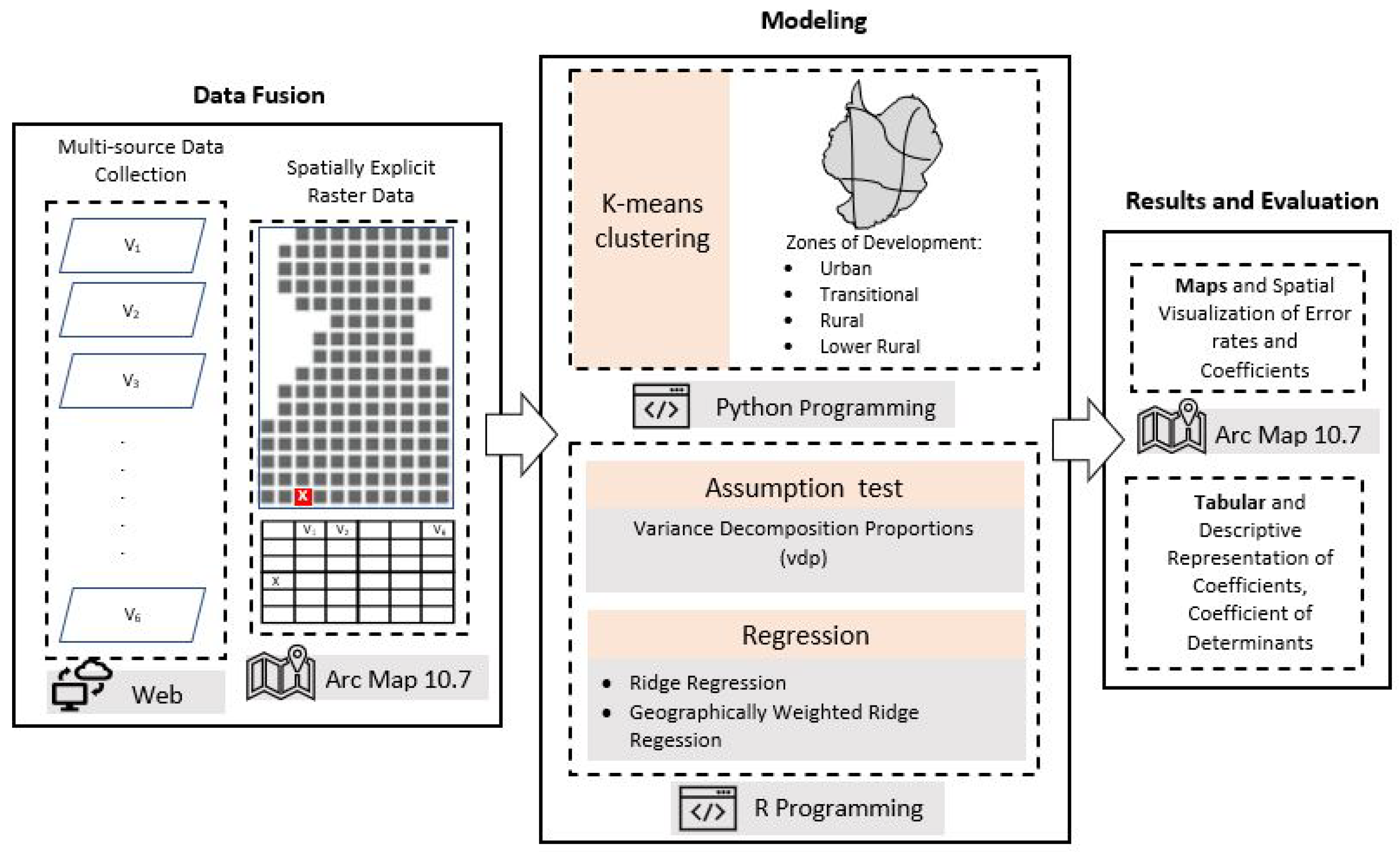
Figure 2 illustrates the methodology of this research. This framework utilizes local and global regression coefficient analysis. ArcMap 10.7 and R programming language were used to implement the models. An integration of place-based and global variables was deployed in the time period of 1985−2015 with ten-year time-steps. The ten-year time intervals allow access to corresponding census and economic data and study them in connection with the landscape change. This section is designed to set forth the methods in the case study of West Virginia.

3.1. Study Area

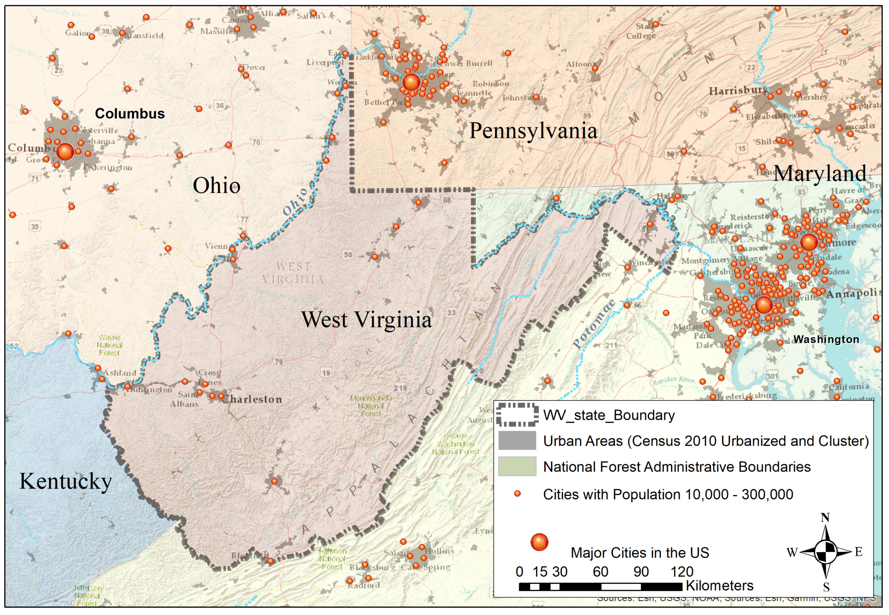
The study region of WV (Figure 3), with an area of 62,259 km 2 is completely within the defined extent of the Appalachian Mountains [23]. The terrain and topographic characteristics, and rich natural assets create a unique context for the anthropogenic activities in this region. WV has abundant physical and environmental assets. Energy extraction industries play a crucial role in the economy of WV; coal was one of the primary natural resources of the state. Since early 2000s, shale gas extraction sites have expanded in WV [24]. The Monongahela National Forest with a land area of over 3719.06 km 2 is located in the south-east of WV [25]. This state is the major water source of large rivers such as the Potomac and Ohio rivers. This state has a northern and an eastern panhandle. Jefferson county, one of the 55 counties of this state in the eastern panhandle, is in the Washington DC Metropolitan Statistical Area (Metropolitan Statistical Areas (MSA) are defined by the U.S. Office of Management and Budget (OMB) and used by the Census Bureau and other federal government agencies in the United States (US) for statistical purposes. An MSA consists of one or more counties that contain a city of 50,000 or more inhabitants, or contain a Census Bureau-defined urbanized area (UA) and have a total population of at least 100,000 (75,000 in New England) [26].). The north central WV borders the Pittsburgh, PA, MSA. Both Pittsburgh and DC MSAs are populated regions with substantial number of organizations in the industrial and administrative sectors. Energy extraction industries play a crucial role in the economy of WV, the coal industry was one of the primary natural resources of the state. Since the early 2000s, a considerable number of shale gas extraction sites were developed in WV [24]. WV has a unique landscape that, benefits from rich natural and cultural resources. This led to a cycle of economic boom and bust as the value and production through these resources grow and shrink [27].
In the variables section, we describe the studied variables and the patterns of historical land development within the study area.

3.2. Variables

To study the impact of the generic and site-specific factors [6,29] on the process of land development we integrated globally admitted variables with the place-based variables. Place-based factors are the variables that are merely specific to a region [6], global factors refer to the ones that are demonstrated to play an important role in inducing specific landscape transformations in any geography [11,30]. Using different sources of data, the feature class can be constructed. Integrating features from different local, national, and global data sources is accompanied by data formatting and management difficulties. Different geographic reference systems, resolutions, data types, standards and definitions cause such issues. Data fusion methods accommodate dealing with the complexity and heterogeneity of such data [31].
Multi-source spatial data were applied to study the historical trends of land development. Local and federal web-based datasets were used for data acquisition (See Table 1). The main rationale for studying the importance of these variables in the complex and dynamic process of land development was to explore the role of local transitions, along with previously examined variables such as population and economic status [11,30]. On the other hand, studying the multiple hypothetically interacting variables allowed testing the multicollinearity of the variables. Upon identifying the linear relationship between these variables we could examine the application of other models to study the drivers of land development. Within the context of this study, socio-economic, spatial and policy related variables of urban and rural land development create a dynamic and complex system of changes [29,32]. We also used distance to an existing land development as a human made physical variable. A spatially explicit model was applied, meaning that we used distance, density, and data interpolation to construct the input data. We used census population data at the census tract level in each decade. The economic status was represented using the County Economic Status Index proposed by the Appalachian Research Commission (ARC) [23]. This index is a linear factor of household poverty rate, per capita income, and unemployment rate. Economic index is defined and applied by ARC to indicate the economic status of this region. We used ARC’s method to compute the economic index (E.I.). In Table 1 the explanatory variables that we used, the input data, and the data source are listed. We verified that the data was geo-referenced and co-registered.
In Table 2 the summary statistics of the variables are included, this summary statistics is based on the variables’ values before pre-processing. The variables in this work are integrated so the information is scaled, geo-referenced, and co-registered, and the data layers are temporally and spatially synchronized. The pre-processing steps of variables included scaling and interpolation. Scaling the variables helps in making an explicit analysis and improving the stability and performance of the regression models. We scaled the variables by conducting a min-max normalization, where the minimum value of each feature is subtracted and the result is divided by the range. We used the inverse distance values; so the closer the features are to active mining sites, shale gas wells, metropolitan areas, and other forms of development the larger the value of that variable is.
The data of the historical land development in WV is acquired from [35]. Thirty meters resolution Landsat images were utilized to obtain these images. We used six spectral bands from red, green, blue, near-infrared, and short wave near infra-red sensors for both TM5 and TM8 satellite images.These images are collected in the ±1-year interval of the target year. A pairwise analysis from each scene is conducted on the normalized dataset, any pair is analyzed independently. A total number of 10 scenes cover the entire state of WV, a hybrid algorithm was used in which data transformation and band differencing were deployed. Using this algorithm, a new feature class of the Landsat satellite images was constructed, and an unsupervised machine learning model was applied to group the cells in the reconstructed feature class. [35] labeled the grouped data of land cover using k-means algorithm. Historical data of google earth was utilized as the ground truth to validate the results [35]. The output of this study provides the data of historical trends of land development for each decade of 1985−1995, 1995−2005, and 2005−2015 (Figure 4).
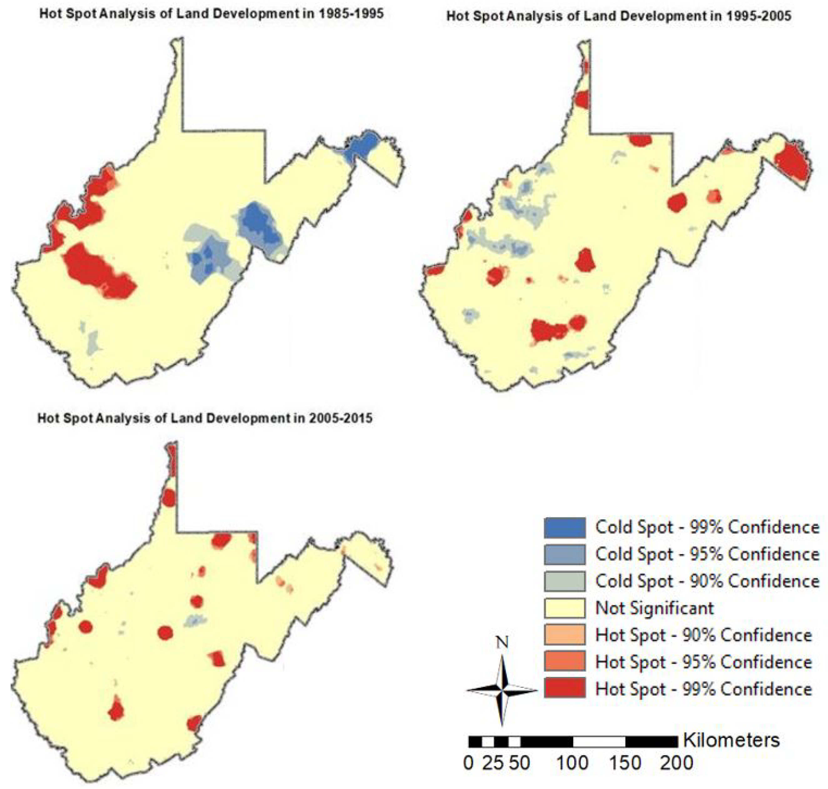
The data of Figure 4 is applied for hot spot analysis of land development [36]. Hot spot analysis indicates the dynamics and patterns of land development. This method is used to identify statistically significant spatial clusters of new land developments [36]. Through this analysis the patterns of the new land developments have been identified. The hot spots (Figure 5) are the regions wherein there are high clusters-high density new developments. Cold spots are the region in which the clusters of low density new developments were formed.
Spatial auto-correlation is used to test for statistically significant spatial auto-correlation in the geographic events [8]. To find the distance at which the clusters of new land developments were more intense a spatial auto-correlation analysis was conducted. Within this distance, the density of events was compared to a complete random pattern of new land developments and the G i * statistic was computed for each new development event (Equation (4)). These values represent a z score per feature in the study area [8].
G i * = j = 1 n w i , j x j X ¯ j = 1 n w i , j S [ n j = 1 n w i , j 2 ( j = 1 n w i , j ) 2 ] n 1
where, x j is the number of collected events in one k m 2 , w i , j is the spatial weight between feature j and i, n is the total number of collected event points. We used Inverse Distance Weighting (IDW) to acquire the w i , j values, IDW computes the weights based on the assumption that the near features are more related than the distance ones (Tobler’s First Law of Geography [37]). X ¯ and S are formulated in Equations (5) and (6):
X ¯ = j = 1 n x j n
S = j = 1 n x j 2 n X ¯
IDW was applied to interpolate the z score of the G i * statistic of each event point to the cells in the region. This technique provides a good understanding of the new development patterns by assessing both density and the extent of interaction between the events [38]. The interpolated values were used as the dependent variables in this study. Figure 5 illustrates the interpolated z score of the G i * statistic, positive z score values show clustered high-density new land developments and negative z scores show clusters of low-density new land developments. High z scores mainly show up around the major cities and low clusters represent scattered developments in the rural areas.

3.3. Assumption Test and Modeling

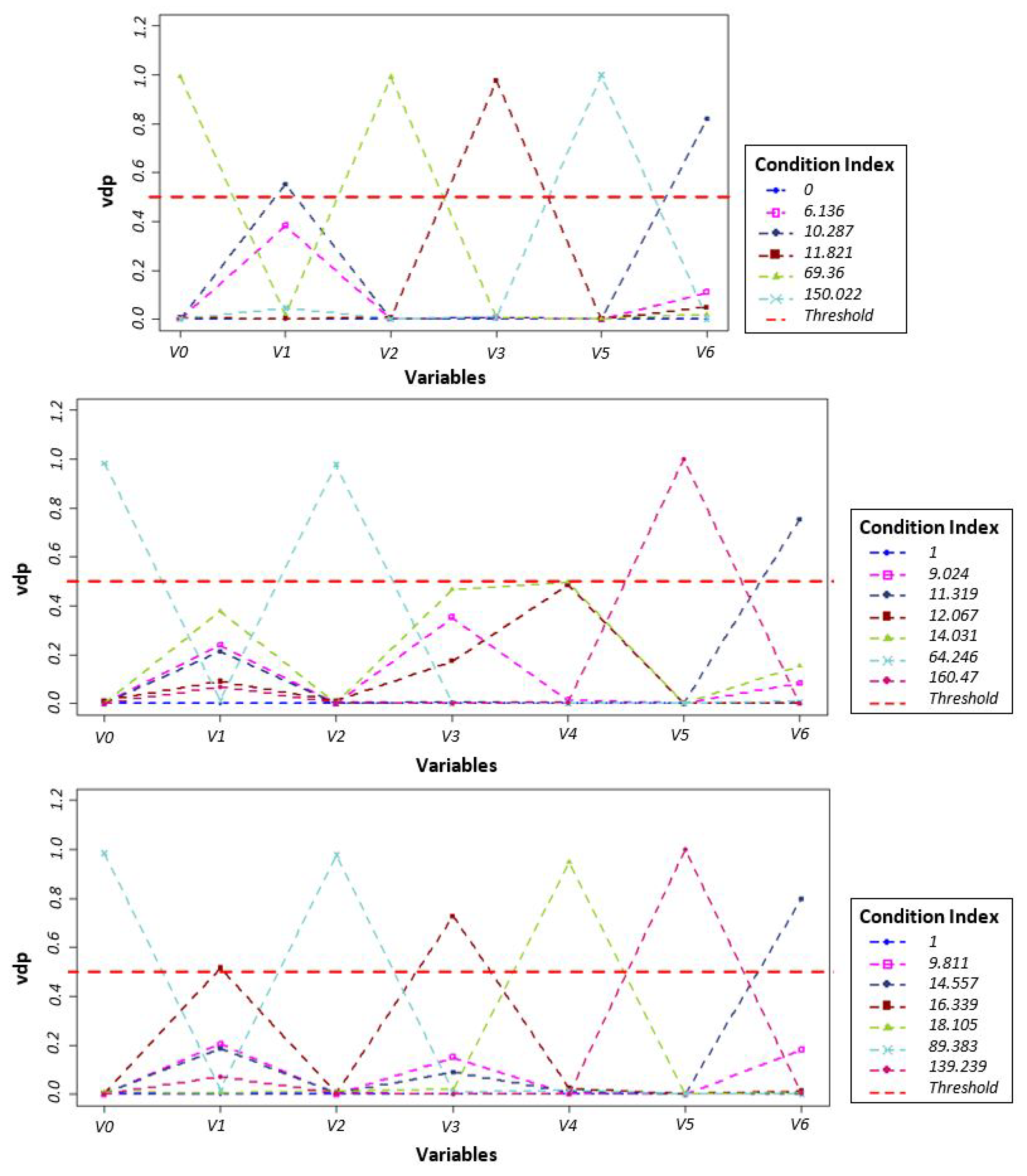
As a requirement for the modeling, we performed an assumption test (discussed in Section 2.2). Through this test we studied the C I (Equation (1)) and v d p values to find out if there is a multicollinearity among the variables. As suggested by [21] a C I of greater than 10 represents a moderate to severe degree of collinearity. They also imply that researchers have variety of criteria for a high v d p , however, the most common threshold is a v d p of 0.50 or greater for two or more variables associated with a high C I [21]. Hence, to detect the multicollinearity of the variables, tolerance value of 10 for C I and 0.5 for the v d p were assigned. The decomposition values which are above the threshold and have the C I of more than 10 represent the multicollinearity. Figure 6 shows the presence of global multicollinearity in all three studied time-steps. In this figure we can observe that in any of the global regression models there are multiple variables that present a multicollinearity with other ones.
We used the same method for multicollinearity diagnostics in the local OLS regressions (Figure 7). Considering that local regression analysis encompasses multiple OLS models, in Figure 7 maximum value of v d p for each regression model is represented and the v d p values that are above the threshold indicate presence of multicollinearity in the model. This analysis confirms presence of local multicollinearity between the variables in all time-steps (Figure 7). To avoid the drawbacks of local and global multicollinearity in regression models (discussed in Section 2.3), ridge regression was utilized. We used a 10-fold cross validation to compute the value of model hyperparameter in both ridge regression and GWRR models.
The optimum bandwidth value for the GWRR model was computed using an exponential distance kernel (See Table 3). Our inferences are based on the GWRR coefficients of each variable and we did not compare the results for each variable with another. The range of coefficients among the variables is considerably different, this variance is because of significance of one variable over another, high dynamics of variables across the region and over time, and the model fitting process in the GWRR.

3.4. Model Evaluation

Coefficient of determination, denoted as R 2 (Equation (7)) is widely used for evaluating regression model performance [15].
R 2 = 1 i ( y i f i ) 2 i ( y i y ¯ ) ) 2
where, y i is the actual value of z score per event, y ¯ is the mean value of the z scores and f i is the predicted value of the z score for new developments. Coefficient of Determination is one of the measures of model accuracy that we used in this study. We used other statistics to obtain insights on the model performance.
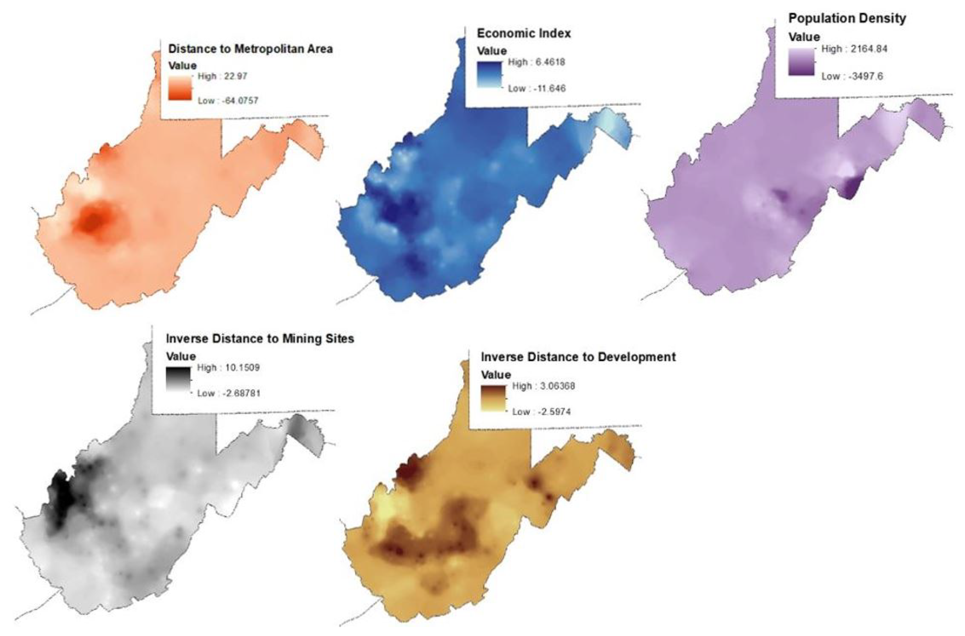
t and p values of each variable are utilized to evaluate the significance of coefficients in the ridge regression models. In addition, the scaled estimates of each parameter, which points to its proportional significance, is also computed. In our local analysis of the variables, each event has its own summary statistics. Therefore, we found pictorializing an innovative method to analyze and evaluate the local regression models. The difference of estimated and actual z score values of each event point is depicted to show how the error of local regression models are distributed in the study area. Moreover, the parameters of the local regressions are represented in the geographic format. The coefficient values of each event point were interpolated using IDW operation to generate such raster graphics.
IDW method is used in studying the spatial patterns of land development (see Section 3.2)), making visual inference on GWRR coefficient results (see Section 4.2), and on visualizing GWRR coefficient results (see Section 4.2). To validate the IDW results, we used a 10% random sample and excluded them form the IDW analysis and conducted the interpolation. Then the interpolated values at the validation subset were compared to the actual values. The residuals of the IDW were computed using Mean Squared Error (MSE), we used this method to identify optimum search radius and power of inverse distance weighting. These values are computed based on the minimum MSE.
In addition, we investigated the geography of the model residuals (Equation (8)). Through this study the residuals of GWRR models are depicted in the study area.
S q E r r = ( y i ^ y i ) 2
where, S q E r r is the Squared Error value, y i ^ is the estimated value for the i th event and y i is its actual z score value.
Moreover, providing zonal references for an expressive discussion is extremely helpful to discussing the model output. Therefore, we deployed a visual representation of the zones of development based on four zones of development of lower rural, rural, transitional and populated/urbanized zones. We discuss the process of identifying the regions of development in Section 3.4.1.

3.4.1. Zones of Development

Zones of development are identified according to the density of development and population in each census tract. The classes of this data are: populated/urbanized, transitional area, rural, and lower rural. Clustering of the tracts is performed using the k-means method. The urbanized/populated areas point to the regions with higher density of development and populated places. The areas denoted as the transition areas, are either the immediate areas surrounding the urban areas in which the population density was higher than the rural area, or some areas that are initial cores for dense population settlements in the future development. Rural areas and lower rural areas are mainly regions with scattered developed lands and dispersed population, the level of sparsity varies between rural areas and lower rural regions. After clustering, we applied Multivariate Analysis of Variance (MANOVA) to test the significance level of the difference between the groups (See Table 4). The homogeneity of the variables across the grouped data was then tested, the results of this test imply that all the clusters are significantly different from each other.
Figure 8 illustrates zones of development, according to this analysis, the area of urban and transitional zones in the three target time periods of the study was less than 15% of the state. By overlaying the zones of development on top of the hot-spot analysis of new developments, we can observe that the hot spots are formed in the urban and transitional regions. We basically use the zones of development to make visual inferences on the results of geographically weighted regression models.

4. Results

4.1. Global Ridge Regression Model

The global ridge regression model of land development at each time-step indicates R 2 of 0.61, 0.70 and 0.69 for 1985−1995, 1995−2005, 2005−2015, respectively. The parameters of variables for the global ridge regression are shown in Table 5. The global regression models indicate that in 2005−2015 distance to mines do not demonstrate a significant impact on the land development.
According to a study by the Bureau of Business and Economics in the state of WV [24], during this period, there was a decrease in jobs and mining production. However, at this time-step oil and gas industry acts as the substitute to mining in WV. As Table 5 shows, distance to mining sites was an important driving factor for land development in 1985−1995. In the period of 1995−2005, population density was the most significant variable in land development in WV. In 1985−1995 this factor is not as important compared to other factors.

4.2. Geographically Weighted Ridge Regression Model Results and Visual Assessment

A geographical regression model was done and the evaluation of model performance (See Table 6) shows the R 2 value for each model. The value of R 2 for the GWRR models is computed based on Equation (7), where the estimated values are the model prediction for each weighted regression model.
An interpolation in the squared error of GWRR models points to the spatial representation of the model performance (Figure 9). Indeed, this figure indicates the areas where the regression model fits better to the training points or fails to explain the land transformation with the presented variables. The value of squared error, in each GWRR model varies, such that the 1985−1995 GWRR has the smallest range of error rate and 1995−2005 GWRR has the highest range of error.
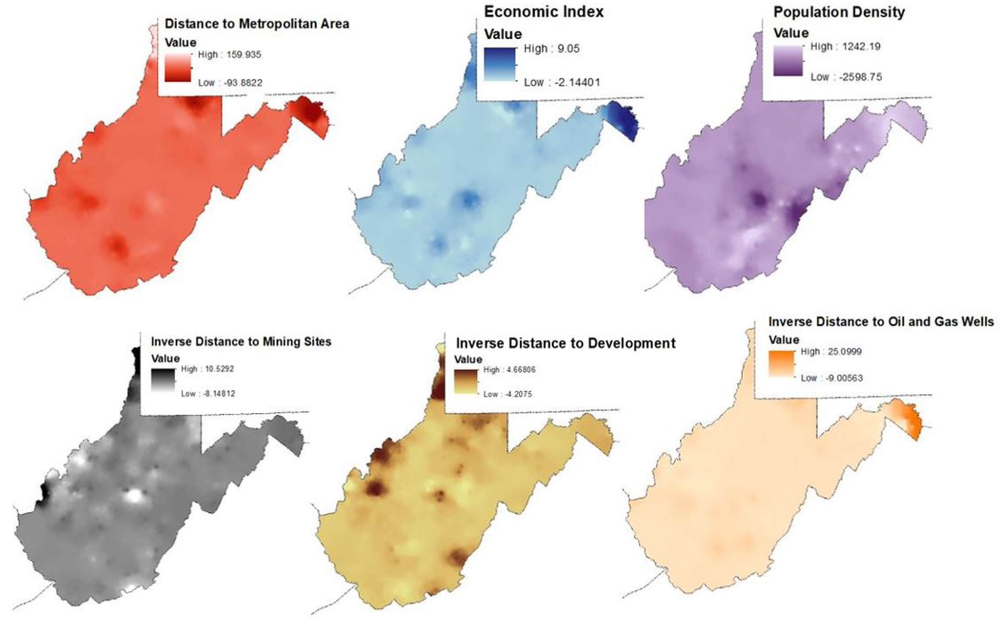
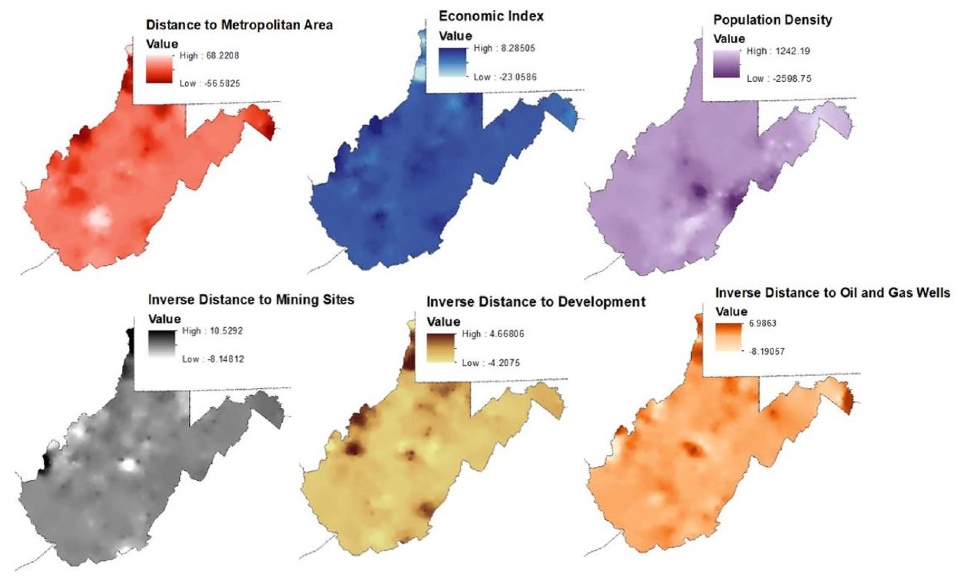
The geographic coefficients of each variable in 1985−1995 imply high impact of the variables on the western and central WV. Charleston (state capital) and Parkersburg MSAs are located in these regions. Nevertheless, it is noteworthy that hot spots of land development and the highest error rates are detected in these regions. This shows that our model is not capable of capturing the local relationships between the variables in these hot spots that are mainly urban and transitional regions. Changes in the population density has almost the same impact on the clusters of development in all the regions except for the east of the state; which is mainly in the vicinity of the Monongahela National Forest with regulatory restrictions on land development. Moreover, the model result confirms any change in the population of the mentioned region is accompanied by significant changes in the clusters of land development (Figure 10). Our dataset indicates no records on active permits of oil and gas wells, hence we did not investigate this variable in 1985−1995.
Taking the high and low error regions into consideration, we can make more reliable inferences on the local regression parameters. Model parameters for 1995−2005 (Figure 11) indicate that changes in the economic index and distance to mining areas exhibit notable influence on the developed land clusters. Distance to oil and gas wells and mining sites significantly impact land development in the eastern panhandle of the study area. The metropolitan areas of Charleston and Parkersburg show substantial linkages to changes in distance to oil and gas wells, and population change and distance to development.
Local coefficients in 2005−2015 indicate that the land development process is impacted by the oil and gas industry in a large geography. This change is because of the population movement caused by the job opportunities that these industries create. On the other hand, oil and gas industries in this region are mainly based on shale gas wells. These sites require considerable land areas for side facilities and the pipelines [28]. Population density has comparatively higher coefficient value in the very low populated and rural areas. In the northern and eastern panhandles, the model parameters indicate that distance to metropolitan areas play a crucial role in the formation of new land developments (Figure 12).

5. Discussions

5.1. Study Findings

The results of this investigation in the state of WV imply that the majority of detected land developments in all the three time-steps occurred in rural and lower rural areas. Nonetheless, the importance of the studied variables on land development process have been constantly shifting. Without performing the local analysis of this research, it would suffer from lack of evidence for studying this dynamicity. Local analysis of the variables helped us to gain insight into the locations where the parameters act quite opposite from each other. Since we did a separate data normalization for each variable per time-step, our inferences on the importance of each variable is made in target time-step are independent from each other.
We incorporated the temporal change of geography of opportunities by representing distance-based spatial features. Both global and local analysis indicate that the location of opportunities plays a vital role in driving land development. In the short time period of 1985−2015 we have observed how the dynamics of geography of opportunities have shifted the patterns of land development. The dynamic patterns of economic opportunities over time lead to unstable trends of urban/rural land development. These ephemeral patterns hinder small, low populated communities and provoke fragmented localities.
Major land transformations were observed in rural regions (Figure 5 and Figure 8), where the pattern of land development is scattered, with low and very low clusters of developed and populated lands. This form of development in a region which is covered by forested lands (according to NLCD 2016 more than 84% of WV is forested [5]) results in an impacted ecosystem. On the other hand, the need of these fragmented communities, which are rapidly growing and shrinking, to access health, commercial, social, educational, and cultural services is a major concern. A shortage of access to these services impacts the residents’ quality of life.
The energy industry is one of the major reasons for the landscape alterations in WV [27]. As some energy sources diminish or lose their popularity, it impacts the patterns of land development; in this case, the older developed areas do not provide enough incentives to sustain the trends of land development. This indicates that this region could not maintain the provided opportunities for the job seekers and the geography of opportunities was mutating.

5.2. Implications

This study provides a foundation for examining the scenarios and consequences of land development on ecosystem services. We recommend such studies to be conducted and reviewed with the communities. Moreover, enriching and educating communities with sustainable economic development, instead of relying of transitory economic industries should be considered in planning the future in such regions. Community engagement steps are encouraged for the sustainability of development in this region.
As indicated by this work, land and natural resources of energy are key role players in the landscape alterations of WV. Understanding how land development in WV also impacts various aspects of ecosystem services is critical. Mapping, monitoring, and publicly discussing the land transformation’s impacts on regulating, provisioning, cultural and supporting ecosystem services facilitates public awareness of the environmental consequences of each act of land consumption.
Future research should attempt to apply the methodology presented here to other study areas and other forms of land transformation. It is important to incorporate local knowledge for characterising and determining explanatory variables. For example, other factors such as terrain characteristics i.e., topography, land supply and demand, governmental policies, local pricing and markets, etc. should be considered. In addition, future work could investigate the use of other models such as feature selection methods and deep neural networks.

6. Conclusions

This research examined the significance of multiple variables in the land transformation process. We applied fused multi-source data to build the feature class for the geographically weighted and global ridge regressions. Through the proposed method, the presence of multicollinearity among variables was tested and the modeling process was improved. We implemented the models and analyzed the data in decennial time steps.Both local and global ridge regression models were used. In the local ridge regression, as in the global ridge model, penalizing the loss values helped avoid a multicollinearity effect. This helped address the problem of over-fitting. We used the results of this study to infer the role of the energy sector on the land development in the study area. Also, the process of land development in the study area is essentially fragmented and scattered. We provided recommendations on the community development and public guidelines and strategies so the future land developments in the region can move in a more sustainability and resilient direction.

Author Contributions

Conceptualization, P.P., M.P.S., M.J.D. and D.A.A.; Data curation, P.P.; Formal analysis, P.P.; Funding acquisition, M.P.S.; Investigation, P.P.; Methodology, P.P., M.P.S., M.J.D. and D.A.A.; Project administration, M.P.S. and M.J.D.; Resources, M.P.S.; Software, P.P. and M.P.S.; Supervision, M.P.S., M.J.D. and D.A.A.; Validation, P.P., M.P.S. and M.J.D.; Visualization, P.P.; Writing—original draft, P.P.; Writing—review & editing, P.P., M.P.S., M.J.D. and D.A.A. All authors have read and agreed to the published version of the manuscript.

Funding

This effort was supported by the National Science Foundation under Cooperative Agreement Number OIA-1458952. Any opinions, findings, and conclusions or recommendations expressed in this material are those of the author(s) and do not necessarily reflect the views of the National Science Foundation. This work was also supported by the USDA National Institute of Food and Agriculture, Hatch project accession number 1015648, and the West Virginia Agricultural and Forestry Experiment Station. We would also like to acknowledge the anonymous reviewers who helped to improve this work.

Institutional Review Board Statement

Not applicable.

Informed Consent Statement

Not applicable.

Data Availability Statement

Data available in publicly accessible repositories cited in the paper.

Conflicts of Interest

The authors declare no conflict of interest to disclose.

References

  1. De Groot, R. Function-analysis and valuation as a tool to assess land use conflicts in planning for sustainable, multi-functional landscapes. Landsc. Urban Plan. 2006, 75, 175–186. [Google Scholar] [CrossRef]
  2. Foley, J.A.; DeFries, R.; Asner, G.P.; Barford, C.; Bonan, G.; Carpenter, S.R.; Chapin, F.S.; Coe, M.T.; Daily, G.C.; Gibbs, H.K.; et al. Global consequences of land use. Science 2005, 309, 570–574. [Google Scholar] [CrossRef] [PubMed] [Green Version]
  3. Bürgi, M.; Hersperger, A.M.; Schneeberger, N. Driving forces of landscape change-current and new directions. Landsc. Ecol. 2005, 19, 857–868. [Google Scholar] [CrossRef]
  4. Anderson, J.R. A Land Use and Land Cover Classification System for Use with Remote Sensor Data; US Government Printing Office: Washington, DC, USA, 1976; Volume 964.
  5. NLCD Classes of Landcover. Available online: https://www.mrlc.gov/data/legends/national-land-cover-database-2016-nlcd2016-legend (accessed on 29 March 2021).
  6. Lambin, E.F.; Turner, B.L.; Geist, H.J.; Agbola, S.B.; Angelsen, A.; Bruce, J.W.; Coomes, O.T.; Dirzo, R.; Fischer, G.; Folke, C.; et al. The causes of land-use and land-cover change: Moving beyond the myths. Glob. Environ. Chang. 2001, 11, 261–269. [Google Scholar] [CrossRef]
  7. Wheeler, D.C. Diagnostic tools and a remedial method for collinearity in geographically weighted regression. Environ. Plan. A 2007, 39, 2464–2481. [Google Scholar] [CrossRef]
  8. Getis, A.; Ord, J.K. The analysis of spatial association by use of distance statistics. In Perspectives on Spatial Data Analysis; Springer: Berlin/Heidelberg, Germany, 2010; pp. 127–145. [Google Scholar]
  9. Sheehan, K.R.; Strager, M.P.; Welsh, S.A. Advantages of geographically weighted regression for modeling benthic substrate in two Greater Yellowstone ecosystem streams. Environ. Model. Assess. 2013, 18, 209–219. [Google Scholar] [CrossRef]
  10. Ren, Y.; Lü, Y.; Fu, B.; Comber, A.; Li, T.; Hu, J. Driving Factors of Land Change in China’s Loess Plateau: Quantification Using Geographically Weighted Regression and Management Implications. Remote Sens. 2020, 12, 453. [Google Scholar] [CrossRef] [Green Version]
  11. Maimaitijiang, M.; Ghulam, A.; Sandoval, J.O.; Maimaitiyiming, M. Drivers of land cover and land use changes in St. Louis metropolitan area over the past 40 years characterized by remote sensing and census population data. Int. J. Appl. Earth Obs. Geoinf. 2015, 35, 161–174. [Google Scholar] [CrossRef]
  12. Mennis, J. Mapping the results of geographically weighted regression. Cartogr. J. 2006, 43, 171–179. [Google Scholar] [CrossRef] [Green Version]
  13. Huang, X.; Huang, X.; Liu, M.; Wang, B.; Zhao, Y. Spatial-temporal dynamics and driving forces of land development intensity in the western China from 2000 to 2015. Chin. Geogr. Sci. 2020, 30, 16–29. [Google Scholar] [CrossRef] [Green Version]
  14. Aguayo, M.I.; Wiegand, T.; Azócar, G.D.; Wiegand, K.; Vega, C.E. Revealing the driving forces of mid-cities urban growth patterns using spatial modeling: A case study of Los Ángeles, Chile. Ecol. Soc. 2007, 12, 13. [Google Scholar] [CrossRef]
  15. James, G.; Witten, D.; Hastie, T.; Tibshirani, R. An Introduction to Statistical Learning; Springer: Cham, Switzerland, 2013; Volume 112. [Google Scholar]
  16. Klein, L.A. Sensor and Data Fusion: A Tool for Information Assessment and Decision Making; SPIE Press: Bellingham, WA, USA, 2004; Volume 138. [Google Scholar]
  17. Zhu, A.X.; Band, L.E. A knowledge-based approach to data integration for soil mapping. Can. J. Remote Sens. 1994, 20, 408–418. [Google Scholar] [CrossRef]
  18. Blasch, E.; Lambert, D.A. High-Level Information Fusion Management and Systems Design; Artech House: Norwood, MA, USA, 2012. [Google Scholar]
  19. Warner, T.; Almutairi, A. Chapetr 33: Remote sensing and land cover change. In The SAGE Handbook of Remote Sensing; SAGE: Thousand Oaks, CA, USA, 2009; pp. 459–472. [Google Scholar]
  20. Cornell, J.A. Classical and Modern Regression with Applications; Taylor & Francis Group: Oxfordshire, UK, 1987. [Google Scholar]
  21. Callaghan, K.J.; Chen, J. Revisiting the collinear data problem: An assessment of estimator’Ill-Conditioning’in linear regression. Pract. Assess. Res. Eval. 2008, 13, 5. [Google Scholar]
  22. Esri, National Atlas of the United States, United States Geological Survey, Department of Commerce, Census Bureau, Geography Division, USA. Available online: https://www.arcgis.com/ (accessed on 29 March 2021).
  23. Appalachia Regional Commission, USA. Available online: https://www.arc.gov/research (accessed on 29 March 2021).
  24. Annual report of the United Nations High Commissioner for Human Rights and reports of the Office of the High Commissioner and the Secretary-General. In Economic Impact of Energy and Environmental Policy in Appalachia; Appalachian Regional Commission: Washington, DC, USA, 2011.
  25. US Geological Survey, USA. Available online: https://waterdata.usgs.gov/wv/nwis/current (accessed on 29 March 2021).
  26. U.S. CensusUS Geological Survey, USA. Available online: https://www.census.gov/ (accessed on 29 March 2021).
  27. Ghadimi, H. Sustainable Economic Development Planning in Energy Rich Regions. J. Energy Dev. 2015, 41, 68–84. [Google Scholar]
  28. GIS Tech Center at West Virginia University, Morgantown, WV, USA. Available online: http://wvgis.wvu.edu/ (accessed on 29 March 2021).
  29. Verburg, P.H. Simulating feedbacks in land use and land cover change models. Landsc. Ecol. 2006, 21, 1171–1183. [Google Scholar] [CrossRef]
  30. Huang, Z.; Wei, Y.D.; He, C.; Li, H. Urban land expansion under economic transition in China: A multi-level modeling analysis. Habitat Int. 2015, 47, 69–82. [Google Scholar] [CrossRef]
  31. Liu, J.; Li, T.; Xie, P.; Du, S.; Teng, F.; Yang, X. Urban big data fusion based on deep learning: An overview. Inf. Fusion 2020, 53, 123–133. [Google Scholar] [CrossRef]
  32. Pato, R.L.; Castro, P.; Tavares, A.O. The relevance of physical forces on land-use change and planning process. J. Environ. Plan. Manag. 2016, 59, 607–627. [Google Scholar] [CrossRef] [Green Version]
  33. USGS Earth Explorer, USA. Available online: https://earthexplorer.usgs.gov/ (accessed on 29 March 2021).
  34. U.S. Bureau of Labor, USA. Available online: https://www.bls.gov/ (accessed on 29 March 2021).
  35. Pourmohammadi, P.; Adjeroh, D.A.; Strager, M.P. Mapping the Land Development Processes Using Data Transformation and Clustering Methods. In Proceedings of the IGARSS 2020—2020 IEEE International Geoscience and Remote Sensing Symposium, Waikoloa, HI, USA, 26 September–2 October 2020; pp. 2775–2778. [Google Scholar] [CrossRef]
  36. Mitchell, A. The ESRI Guide to GIS Analysis (Volume 2); Esri Press: Redlands, CA, USA, 2005. [Google Scholar]
  37. De Smith, M.J.; Goodchild, M.F.; Longley, P. Geospatial Analysis: A Comprehensive Guide to Principles, Techniques and Software Tools; Troubador Publishing Ltd.: Kibworth, UK, 2007. [Google Scholar]
  38. Scott, L.M.; Janikas, M.V. Spatial statistics in ArcGIS. In Handbook of Applied Spatial Analysis; Springer: Berlin/Heidelberg, Germany, 2010; pp. 27–41. [Google Scholar]
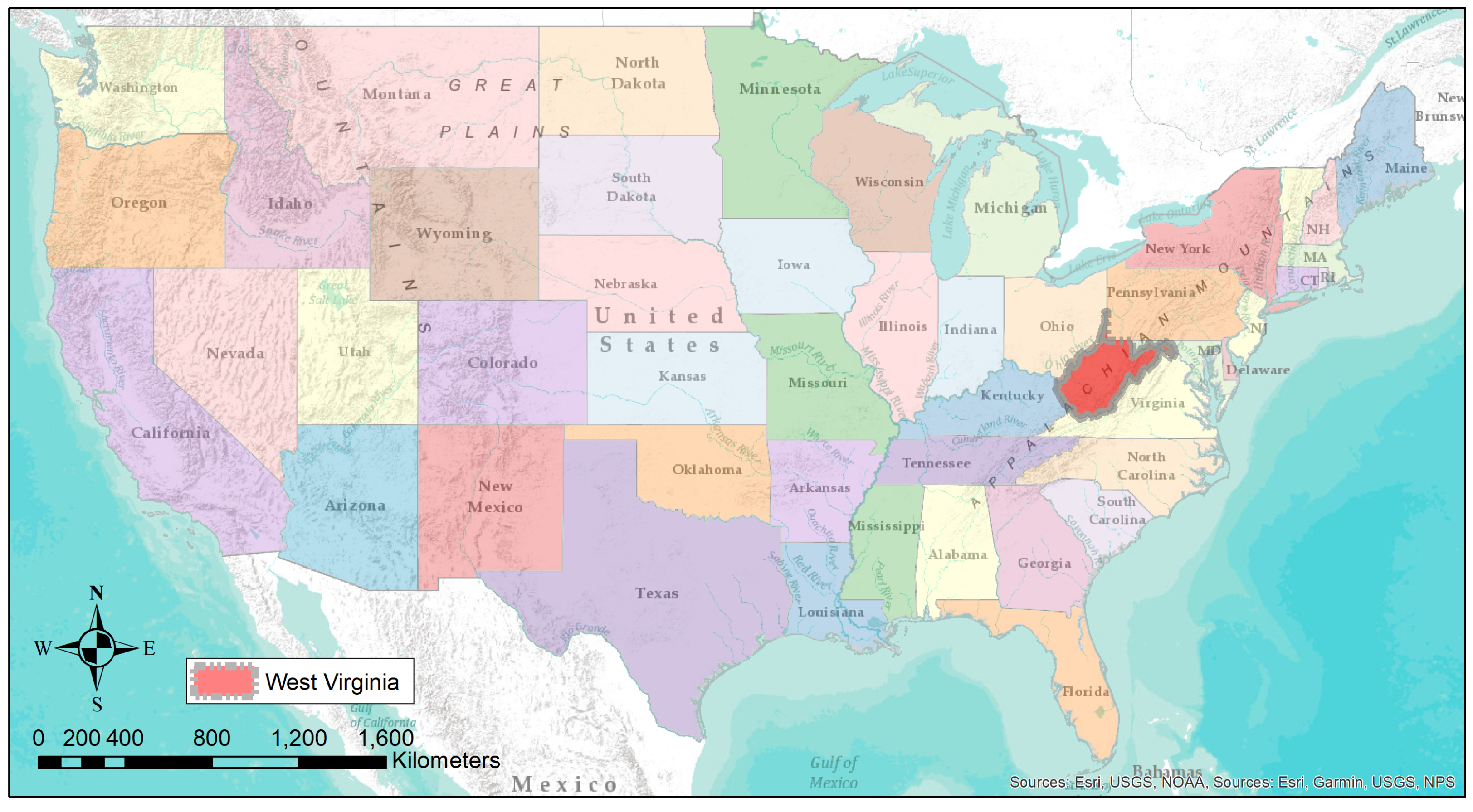
Figure 1. West Virginia (WV) State in the US (Data Source [22]).
Remotesensing 13 01307 g001
Figure 2. Methodology of the study; The variables comprise of a combination of place specific variables, (i.e., distance to energy extraction sites), socio-economic variables, distance to other forms of land development, and distance to Metropolitan Statistical Areas.
Remotesensing 13 01307 g002
Figure 3. West Virginia State (Data Source [22,28]).
Remotesensing 13 01307 g003
Figure 4. Land development trends in the WV: the right magnified region is Morgantown city, home of West Virginia University and the left on is Charleston, WV’s capital city. These cities are the two most populated MSAs of WV [35].
Remotesensing 13 01307 g004
Figure 5. Hot Spot analysis of land development per decade.
Remotesensing 13 01307 g005
Figure 6. Multicollinearity Diagnostics Analysis of the Variables in OLS Regression Model; V 0 : Intercept, V 1 : Distance to MSAs, V 2 : Inverse distance to developed lands, V 3 : Inverse distance to coal mining sites, V 4 : Inverse distance to shale gas, V 5 : Population density, V 6 : Economic index; Top: 1985−1995, Middle: 1995−2005, Lower: 2005−2015. Variables which demonstrate a condition index of higher than 10 and v d p of greater than 0.5 (threshold line) have multicollinearity.
Remotesensing 13 01307 g006
Figure 7. Multicolleanirity diagnostics analysis of the variables in GWR models.
Remotesensing 13 01307 g007
Figure 8. Zones of Development.
Remotesensing 13 01307 g008
Figure 9. Geography of the Squared-Errors.
Remotesensing 13 01307 g009
Figure 10. Geographic Coefficients for the 1985−1995.
Remotesensing 13 01307 g010
Figure 11. Geographic Coefficients for the 1995−2005.
Remotesensing 13 01307 g011
Figure 12. Geographic Coefficients for the 2005−2015.
Remotesensing 13 01307 g012
Table 1. Studied Variables.
VariableDataSource of Data
Distance to MSA (m)Census DataUS Decennial Census Data [26]
Distance to Developed Land (m)Developed Land Historical TrendsObtained from Landsat [33]
Distance to Mining Sites (m)Mining PermitsWVU GIS Tech Center [28]
Distance to Oil and Gas Wells (m)Shale Gas PointsWVU GIS Tech Center [28]
Population Density (per sq. mile)Census Tract PopulationUS Decennial Census Data [26]
Economic Index (at County Level)Household Poverty Rate (Percentage)US Decennial Census Data and
Per-Capita Income (US $)U.S. Bureau of Labor [26,34]
Unemployment Rate (Percentage)
Table 2. Summary Statistics of the Variables.
1985−1995
VariableData TypeMin.MaxMeanStd. Dev
Distance to MSARaster040,752.168661.128648.79
Distance to Developed LandsRaster04092.55379.29397.15
Distance to Mining SitesRaster0157,53163,558.041,038.9
Population DensityVector1.159.573.902.26
Household Poverty RateTabular/Vector11.1%36.33%20.97%0.06
E.I.Per-Capita IncomeTabular/Vector9422.5018,706.0013,353.412158.46
Unemployment RateTabular/Vector2.96%9.12%5.25%0.02
1995−2005
VariableData TypeMin.MaxMeanStd. Dev
Distance to MSARaster065,662.2715,375.2411,838.02
Distance to Developed LandsRaster04092.55377.20395.75
Distance to Mining SitesRaster042,648.58540.928097.55
Distance to Oil and Gas WellsRaster0167,898.6754,125.0230,187.83
Population DensityVector1.139.703.902.18
Household Poverty RateTabular/Vector9%33.07%17.28%0.05
E.I.Per-Capita IncomeTabular/Vector15,241.1031,342.2020,537.793464.27
Unemployment RateTabular/Vector3.14%12.45%6.56%0.02
2005−2015
VariableData TypeMin.MaxMeanStd. Dev
Distance to MSARaster064,963.9714,732.0412,163.08
Distance to Developed LandsRaster04069.95359.53383.87
Distance to Mining SitesRaster042,648.58111.387476.66
Distance to Oil and Gas WellsRaster0111,511.0315,148.2317,683.43
Population DensityVector1.069.623.952.18
Household Poverty RateTabular/Vector10.30%35.23%19.19%0.05
E.I.Per-Capita IncomeTabular/Vector19,009.5044,424.1030,078.964651.86
Unemployment RateTabular/Vector5.18%13.15%9.17%0.02
Table 3. Model Parameters GWRR.
ModelBandwidth
GWRR 1985−19955801 m
GWRR 1995−20054337 m
GWRR 2005−10154319 m
Table 4. Multivariate Analysis of Variance (MANOVA) test for the zones of developments.
DfPillai’s TraceApprox Fnum Dfden DfPr (>F)Residuals
Zones of Development 198510.787859.052465<2.2 × 10 16 ***466
Zones of Development 199510.76166768.562481<2.2 × 10 16 ***482
Zones of Development 200510.72351629.342481<2.2 × 10 16 ***482
Signif. codes: 0 ‘***’ 0.001 ‘**’ 0.01 ‘*’ 0.05 ‘.’ 0.1 ‘ ’ 1.
Table 5. Summary of Ridge Regression Model Results.
1985−1995
Scaled EstimateStd. Error (scaled)t value (scaled)Pr ( > | t | )
Distance to MSA−1.36380.0170679.95<2 × 10 16 ***
Inverse Distance to Development0.139040.01479.462<2 × 10 16 ***
Inverse Distance to Mining Sites0.550960.0146337.647<2 × 10 16 ***
Inverse Distance to Oil and Gas Wells----
Population Density (per sq. mile)0.168990.0147511.455<2 × 10 16 ***
Economic Index−0.697730.0168741.358<2 × 10 16 ***
Ridge parameter: 8.69 Degrees of freedom: model 4.997, variance 4.994, residual 5
Significance codes: 0 ‘***’ 0.001 ‘**’ 0.01 ‘*’ 0.05 ‘.’ 0.1 ‘ ’ 1
1995−2005
Scaled EstimateStd. Error (scaled)t value (scaled)Pr ( > | t | )
Distance to MSA−40.333220.00817540.76<2 × 10 16 ***
Inverse Distance to Development0.1407290.00752918.69<2 × 10 16 ***
Inverse Distance to Mining Sites0.3413330.00802742.52<2 × 10 16 ***
Inverse Distance to Oil and Gas Wells0.424510.00803552.83<2 × 10 16 ***
Population Density (per sq. mile)0.4475660.0077757.6<2 × 10 16 ***
Economic Index−0.15870.00766820.7<2 × 10 16 ***
Ridge parameter: 38.5 Degrees of freedom: model 5.995, variance 5.991, residual 6
Significance codes: 0 ‘***’ 0.001 ‘**’ 0.01 ‘*’ 0.05 ‘.’ 0.1 ‘ ’ 1
2005−2015
Scaled EstimateStd. Error (scaled)t value (scaled)Pr ( > | t | )
Inverse Distance to MSA−0.44930.00762858.9<2 × 10 16 ***
Inverse Distance to Development0.049350.0066317.4429.95 × 10 14 ***
Inverse Distance to Mining Sites0.0074910.0072861.028 0.303828
Inverse Distance to Oil and Gas Wells0.04090.00914.4956.94 × 10 6 ***
Population Density (in sq mi)0.4004340.00691657.897<2 × 10 16 ***
Economic Index−0.316970.00699245.333<2 × 10 16 ***
Ridge parameter: 65.49 Degrees of freedom: model 5.994, variance 5.987, residual 6
Significance codes: 0 ‘***’ 0.001 ‘**’ 0.01 ‘*’ 0.05 ‘.’ 0.1 ‘ ’ 1
Table 6. Model Results of GWRR.
Model R 2
GWRR 1985−19950.982
GWRR 1995−20050.956
GWRR 2005−10150.961
Publisher’s Note: MDPI stays neutral with regard to jurisdictional claims in published maps and institutional affiliations.