High Spatial and Temporal Resolution Energy Flux Mapping of Different Land Covers Using an Off-the-Shelf Unmanned Aerial System

Abstract

With the development of low-cost, lightweight, integrated thermal infrared-multispectral cameras, unmanned aerial systems (UAS) have recently become a flexible complement to eddy covariance (EC) station methods for mapping surface energy fluxes of vegetated areas. These sensors facilitate the measurement of several site characteristics in one flight (e.g., radiometric temperature, vegetation indices, vegetation structure), which can be used alongside in-situ meteorology data to provide spatially-distributed estimates of energy fluxes at very high resolution. Here we test one such system (MicaSense Altum) integrated into an off-the-shelf long-range vertical take-off and landing (VTOL) unmanned aerial vehicle, and apply and evaluate our method by comparing flux estimates with EC-derived data, with specific and novel focus on heterogeneous vegetation communities at three different sites in Germany. Firstly, we present an empirical method for calibrating airborne radiometric temperature in standard units (K) using the Altum multispectral and thermal infrared instrument. Then we provide detailed methods using the two-source energy balance model (TSEB) for mapping net radiation (Rn), sensible (H), latent (LE) and ground (G) heat fluxes at <0.82 m resolution, with root mean square errors (RMSE) less than 45, 37, 39, 52 W m⁻² respectively. Converting to radiometric temperature using our empirical method resulted in a 19% reduction in RMSE across all fluxes compared to the standard conversion equation provided by the manufacturer. Our results show the potential of this UAS for mapping energy fluxes at high resolution over large areas in different conditions, but also highlight the need for further surveys of different vegetation types and land uses.

1. Introduction

Measuring the surface energy balance is an important task for improving our understanding of land-atmosphere interactions at a time when global climate is shifting towards net warming [1,2,3,4]. The magnitude of warming/cooling through radiative and non-radiative processes is related to land surface properties; for example, dense, tall canopies tend to have relatively low-albedo which causes high energy influx to the system (net radiation, Rn) [5,6]. Decreasing albedo in isolation can have a warming effect, however it can be negated by structural properties such as leaf area index which promote transpiration/latent heat flux (LE) over sensible (H) and ground (G) heat effluxes [1,7,8]. This interplay between Rn, LE, H and G, as moderated by the type, physiology, structure and distribution of vegetation that are present, can influence climate at all scales; from the local scale where shade trees can reduce local temperatures (thus mitigating climatic extremes in agroforestry settings [9]), to regional scale weather systems where the amount and distribution of tree cover can influence precipitation patterns [6,10]. Therefore, the accurate measurement of these fluxes over different land use and land cover types is of great interest to food producers, climatologists and land/water resource managers alike.

Measuring energy fluxes at landscape scale is a non-trivial task. Perhaps the most established technique is via Eddy Covariance (EC). EC stations typically compute Rn using irradiation measurements from pyranometers/net radiometers, H and LE from measuring the covariance between heat and moisture variance and turbulent mixing [11], and G using soil heat flux plates [12]. The method requires integrating high frequency (>10 Hz) gas flux and vertical eddy measurements over 30 min time steps to capture the full range of eddies passing the sensors at different rates (i.e., small eddies move over seconds, large-scale turbulence over minutes). EC stations are usually located in areas of homogeneous vegetation classes within the upwind area (“fetch” or “footprint”) of the tower. Therefore widespread networks of towers are required to capture the variety of fluxes across different vegetation and land cover types which represent the landscape, such as ICOS and TERENO [12,13].

Resistance energy balance models are sound methods used in remote sensing. They rely on the collection of radiometric surface temperature (T_rad) using thermal infrared (TIR) sensors, to effectively cover the survey area of interest. Plant structural and meteorological parameters and T_rad are used as inputs to produce spatially distributed flux estimates. Originally applied to satellite remote sensing data, a number of energy balance models have been successfully adapted for use with very high resolution imagery, either from manned piloted airborne platforms or Unmanned Aerial Systems (UAS). UAS refers to remotely piloted/unmanned aerial vehicles (UAVs) with a sensor mounted on board. With the recent technological advances in miniaturized cameras and navigation systems, UAS are increasingly being used as a more cost-effective and flexible tool in mapping energy and water fluxes, using models such as “mapping evapotranspiration with internalized calibration”, METRIC [14,15], and Two Source Energy Balance model, TSEB [16,17,18,19,20]. To date TSEB is one of the most widely-used spatially-distributed model [21], and has delivered accurate flux estimates using both satellite- and UAS-derived data, independent of resolution [19], in a variety of settings [18,22,23,24,25].

Remote sensing can provide additional information to EC methods. Perhaps most importantly, by using high resolution gridded data, remote sensing can be used to estimate evapotranspiration over individual plants (or plant clusters) [18], and can capture fluxes from different land cover types in one survey [23,26], although many studies have focused on a single vegetation type for testing [21]. Furthermore, the resistance energy methods produce spatially distributed estimates of soil heat fluxes, whereas the EC station ground heat flux plates are fixed to one location, typically near the base of the station [12]. While G can be extrapolated if the vegetation is homogenous, G may vary spatially during in-situ land cover change events (e.g., harvest, mowing or leaf senescence). While the UAS method is not restricted in range by the necessity for homogeneous land cover, the range of the survey area is limited by battery life, local airspace restrictions and air laws, and operations are limited to a narrow window of meteorological conditions (e.g., winds below 9 m s⁻¹). Some platforms have, however, surveyed very large areas in a single flight [27,28]. Typically the reported accuracy of TIR cameras is low, meaning additional control and evaluation steps are often taken to reduce errors caused by internal calibration processes, variability in surface emissivity and atmospheric conditions [18,29,30]. Even though spatially distributed resistance models can only estimate instantaneous fluxes at the pixel scale (compared to EC stations which take measurements 24 h per day, collecting raw data up to 20 times per second) it is still possible to extrapolate hourly/daily flux estimates using remote sensing data [26,31,32]. It should also be noted that some of the constraints of the EC method also apply to the UAS method; both are restricted to flat terrain [13], are limited by sub-optimal meteorological conditions, i.e., atmospheric stability can hinder retrieval of turbulent fluxes [33,34], and both require expert knowledge and experience to collect, process and analyse the data. Additionally, the TSEB model used to estimate the UAS-derived energy fluxes, requires several underlying assumptions in addition to the prerequisites of the EC method, e.g., flux-gradient similarity and accurate knowledge of all non-turbulent surface energy-balance components, including storage terms, which are difficult to measure and therefore often assumed negligible [35]. While UASs are often cheaper than EC stations, they cannot replace EC stations because they provide the most direct method of measuring all major fluxes, whereas UAS can only estimate Rn, H and G, then assign the residual imbalance to LE [7]. Therefore EC methods provide an ideal control for assessing the quality of UAS-derived fluxes [19,36].

Typically, thermal infrared cameras have a lower pixel resolution than standard RGB and multispectral cameras, and as such the tie point-matching algorithms in photogrammetry software (such as Agisoft Metashape and Pix4d) can only function well if there is very high forward and sideward image overlap. This invariably limits the range of the UAV, and consequently the size of the survey area. Some thermal camera manufacturers have integrated an RGB or multispectral camera into the unit so that they have overlapping field of views with the thermal camera [30]. Photogrammetry software can then use the higher resolution optical bands to create accurate thermal orthomosaics. These systems are advantageous because in one single flight a multitude of datasets can be collected (e.g., RGB orthomosaics, vegetation and soil indices, 3D point clouds, as well as radiometric temperature). An example of this system is the Micasense Altum, which has been used for a variety of purposes, including drainage mapping [37], high throughput plant phenotyping [38], bark beetle infestation mapping [39], and vineyard crop health [40]. Many of the existing studies have used thermal infrared cameras mounted on multicopter UAVs, while these platforms can be very versatile, their range can be very limited even without accounting for high image overlap (typically < 20 hectares). The range of fixed wing UAVs can be much greater, however there are operational limitations such as the requirement for large open areas for landing and take-off. Some UASs developed in research institutions (such as the very successful AggieAir system, by [28]) have comprehensive payload sensors (e.g., short, medium, longwave sensors) impressive flight times, and collect scientific standard datasets. Building this kind of system requires expert skills and experience, time, resources and of course money, something not available to many researchers, land and water managers. Several off-the-shelf (OTS) solutions are now on the market aiming to address some of these limitations; some manufacturers have developed vertical take-off and landing (VTOL) fixed wing aircraft which have the take-off and landing flexibility of multicopters, as well as the range advantages of fixed-wing UAVs, with some including integrated RGB/multispectral and thermal infrared cameras. To date few studies have tested their ability to produce reliable and accurate energy flux estimates [21,30], and never with a long-range VTOL UAS.

In summary, there is a wealth of continuous flux data from EC stations across the globe at locations with different land cover types; however resolving the spatial variation in fluxes in areas with mixed vegetation (i.e., heterogeneous plant communities, plant canopy structures etc.) is more challenging. Here, UAS data has the potential to detect and estimate energy and water flux variability at very high resolution, so that we may assess how different land use practices can influence fluxes, the climate and hydrological cycle. An important step in realizing this capability is to calibrate and validate UAS-based fluxes using high-accuracy, directly measured fluxes from EC station in a variety of settings.

This study is the first to demonstrate the capabilities of a long-range, OTS UAS (Quantum Systems Trinity F90+ and Micasense Altum) to map Rn, H, LE and G energy fluxes over different land cover types and report its accuracy and limitations. We provide a detailed methodology for producing energy balance model input datasets that is reproducible across multiple sites with different environmental conditions and plant communities, and present error statistics based on control data from EC stations. Furthermore, we assess two methods of mapping energy fluxes (Two Source Energy Balance Priestley-Taylor, and Dual Time Difference) and report their correlation against three methods of closing the surface energy balance in EC station data.

2. Materials and Methods

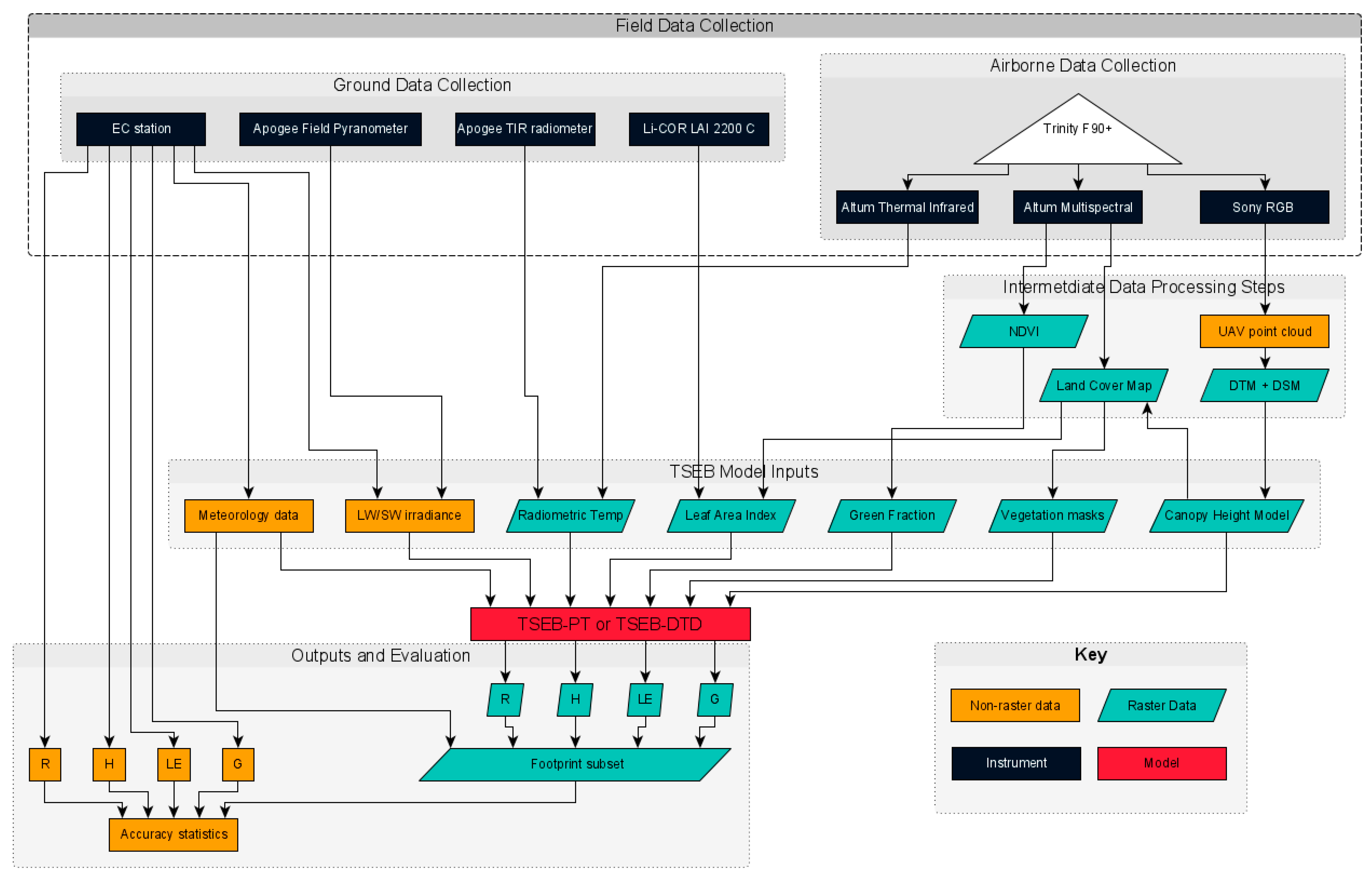
2.1. Methodological Overview

This paper demonstrates a methodology for producing high-resolution spatially distributed energy fluxes using an OTS unmanned aerial system. Fluxes derived from an EC station were used to assess the accuracy of the UAS-derived fluxes by flying the UAS over the “footprint” of the EC station, then comparing the spatially distributed fluxes within the EC footprint with the reported EC estimates for the coincident time period. We use the Two-Source Energy Balance (TSEB) model in this paper and briefly discuss how it calculates the fluxes, however we have not modified the calculations that TSEB performs, therefore a full description of the mechanics behind TSEB can be found in [18] or [7] or [20]. This section will sequentially detail the data collection, processing and evaluation methods as summarized in Figure 1.

2.2. Eddy Covariance Reference Datasets

2.2.1. Eddy Covariance Station Sites

Four different eddy covariance stations across three sites were used to test flux mapping using the UAS. Two EC stations are on grassland sites (Graswang, DE-Gwg [41], and Fendt, DE-Fen [42], which are both operated and maintained by the Karlsruher Institut für Technologie (KIT) network. Full details on the instrumentation can be found in [12]. Mooseurach is a peat bog that was used for forestry until 2016. After several windfall events and increasing bark beetle infestation, the area was cleared. Since then there has been no further management on the area. In addition to the existing 30 m tower (Mooseurach Tall), a 6 m tower (Mooseurach Small) was installed in the former main footprint. This site is part of the ICOS Network [DE-Msr] [43,44], site details and information can be found in

Table 1. Details of the Eddy Covariance Station sites used in this study.

EC Station Name	Elevation (m AMSL)	Location	Vegetation Type	Tower Height (m)	Equipment Used for Flux Measurements
Graswang	869	47.571312° 11.031706°	Grass, Trees	3	LI-7500 1, CSAT3 2, CNR4 3
Fendt	595	47.832905° 11.060738°	Grass	3	LI-7500 1, CSAT3 2, CNR4 3
Mooseurach Small	599	47.809127° 11.457864°	Grass, Shrub, Trees	6	LI-7200 1 CNR4 3, HS-50 4
Mooseurach Tall	599	47.809272° 11.456149°	Grass, Shrub, trees	30	LI-7500 1, CSAT3 2

¹ Infrared gas analyser (LI-COR, Inc., Lincoln, NE, USA). ² Sonic anemometer (Campbell Scientific Inc., Logan, UT, USA). ³ Pyranometer for measuring net radiation (Kipp and Zonen B.V., Delft, The Netherlands). ⁴ Sonic anemometer (Gill Instruments Limited, Lymington, Hampshire, UK).

.

2.2.2. EC Station data and Footprint Delineation

Flux data are calculated over 30 min intervals so that the full range of eddy sizes can be measured. Flux data at Graswang and Fendt were calculated using TK3.1 [45,46,47], whereas data from Mooseurach were calculated using the Eddy-Pro 7.04 by LI-COR Biosciences, (LI-COR Inc., Lincoln, NE, USA). The EC stations at all sites provided supplementary meteorological data, as well as irradiance data as input parameters for the TSEB model.

Footprint delineation provides a spatial component to EC station-based flux estimates so that UAS and EC station-based methods are comparable. For Graswang and Fendt, TK3.1 enables the user to produce a footprint estimation as a spatial probability distribution (in ASCII format) for each 30 min time step using the model by [34]. The performance of the model from [34] that has been used for this study was evaluated by [48] for the Graswang site by a series of controlled tracer release experiments. The results of this study show that it produces realistic footprint estimates. At least for this measurement height and this surface type, the Kormann and Meixner model also agrees well with newer models, such as the FFP model of [49].

Each footprint raster was produced at 1 m resolution, andwas subset using the 98^th percentile because this value consistently produced footprints which largely covered the areas in which the EC stations were situated, and was therefore estimated to provide a representative area in which the mean instantaneous fluxes were estimated from the UAS data (Figure 2).

For Mooseurach, footprint extent estimates are provided in the Eddy-Pro outputs, which include footprint peaks, wind direction, 10, 30, 70, 90% distances. As the weather on the day of the UAS survey was relatively stable with very low wind speeds the footprint statistics were not available for many time steps, so the Mooseurach Small footprint was averaged as a 100 m buffer around the station, and the Mooseurach Tall footprint was delineated using the wind direction limits for the survey period, and maximum distance which overlapped the UAS survey area.

2.3. EC Station Energy Balance Closure

Net radiation (R) is the product of all incoming and outgoing short- and long-wave radiation, and during daytime defines the total energy flux entering the land surface system (minus reflection and emission back into the atmosphere). This energy has three main fates; sensible heat flux (H), the transfer of energy from surface to air (advection) and is transported by convection, latent heat flux (LE), the energy used for evaporation and transpiration of water (or evapotranspiration, ET), and ground heat flux (G), the energy exchange through conduction into the ground heat storage [6,50]. The surface energy balance is summarised by the following equation:

$$Rn=H+LE+G+Imb$$

(1)

where $Rn$ is net radiation, $H$ is the sensible heat flux, LE is the latent heat flux, $G$ is the ground heat flux and $Imb$ refers to an imbalance, which is a residual term if the energy balance is not closed (all in W m⁻²). EC stations measure each individual flux using instrumentation, which often leads to a lack of closure in surface energy balance (Imb) [51]. This can be caused by instrumental errors, errors in the processing chain (pertaining to averaging and flux correction methods), and additional terms that are not measured (canopy heat storage, biochemical storage, horizontal advection, and water pumping by plants) as covered in detail by [52]. To ensure comparability between EC and UAS-derived fluxes and to close the energy balance, we applied four different treatments to the EC station H and LE fluxes, [19,52]:

• No correction
• Increased H and LE to close the energy balance, but maintain the Bowen Ratio (H/LE)
• Added the residual imbalance flux to H, and used uncorrected LE
• Added the residual imbalance flux to LE, and used uncorrected H

2.4. Unmanned Aerial System

2.4.1. Unmanned Aerial Vehicle

We used the Trinity F90+ (Quantum-Systems GmbH, Gilching, Germany), an off-the-shelf (OTS) vertical take-off and landing (VTOL) UAV, with a maximum payload of 500 g. Its VTOL capabilities mean the minimum-required take-off and landing area is approximately 10 m × 10 m; from this small area the UAV launches/lands vertically in “copter-mode”, then transitions to horizontal flight once clear of nearby obstacles. With its optimal 17 ms⁻¹ airspeed, the Trinity F90+ has a maximum flight time of 90 min, meaning it can cover an area of around 150 ha per flight at 100 m above ground level (with 76% sideward image overlap). Flight missions are designed using QBase v2.2.21 software, which links the transmitter, UAS and ground station together via 2.4 GHz wireless connection. QBase has a global digital terrain model and high resolution satellite imagery which allows for precise and safe horizontal and vertical flight path planning. The user can also set up flight spacing and payload sensor triggering to achieve a desired forward and sideward image overlap. The OTS UAS includes a GNSS base station (iBASE, Quantum Systems GmbH, Gilching, Germany) for post processing kinematics (PPK), which can be used to differentially correct image geotags, improving positional accuracy and Structure From Motion (SfM) processing times.

2.4.2. Sensors

We used two airborne sensor payloads for this study (

Table 2. Specifications of the two sensors used in this paper.

Sensor	Bands	Image Resolution (Pixels)	Sensor Size (mm)	Focal Length (mm)	Field of View (°)	Centre Wavelength (nm)	Band Width (nm)	GSD at 100 m Altitude (m)
Micasense Altum	Blue	2064 × 1544	7.12 × 5.33	8	48 × 37	475	32	0.04
	Green					560	27
	Red					668	16
	Red-edge					717	12
	Near Infrared					840	57
	Thermal Infrared	160 × 120	1.92 × 1.44	1.77	57 × 44	11,000	60	0.67
Sony RX1RII	RGB	7952 × 5304	35.9 × 24	35	63	NA	NA	0.01

); the Micasense Altum (Seattle, WA, USA) to produce multispectral (MS) and radiometric temperature orthomosaics and a canopy height model (CHM) for Graswang, and a Sony RX1RII RGB camera to produce a CHM for Mooseurach using structure from motion techniques. The Altum has five high-resolution multispectral bands (blue, green, red, red edge and near infrared) and an integrated long-wave thermal infrared (TIR) sensor (based on the FLIR Lepton) which is aligned with the MS sensors. The Altum has a separate Downward Light Sensor (DLS2, Micasense, Seattle, WA, USA) to provide multispectral calibration information in changing light conditions. The TIR sensor recalibrates every 5 min or when a 2 K change in temperature occurs. The reported accuracy is +/− 5 K with a thermal sensitivity of <50 mK.

2.4.3. Surveys and Flight Parameters

In all, 30 flight surveys (with multiple surveys per flight) were conducted between 20 July 2020 and 20 October 2020, and a summary of the flight details can be found in

Table 3. Summary of flight times, simple meteorology, and number of images acquired per flight (note that this refers to the number of 6-band images).

Location	Date	Time	Duration (Minutes)	Weather	Air Temperature (°C)	Survey Area Overpasses	Images Taken	Average Flying Height (m AGL)
Graswang	20 July 2020	12:00	20	Sunny	25.8	1	382	100
		12:30	20	Sunny	26.0	1	566
		13:30	40	Sun/cloud	26.4	2	863
Graswang	15 September 2020	07:15	40	Sunny	18.0	2	818	120
		10:00	40	Sunny	25.9	2	756
		11:30	40	Sunny	27.9	2	775
		13:30	40	Sun/cloud	28.0	2	754
Fendt	17 September 2020	07:30	30	Overcast	19.9	1	837	110
		08:30	30	Overcast	21.0	1	842
		10:30	40	Sunny	21.0	2	738
		11:15	20	Sunny	24.5	1	482
		12:30	40	Sunny	26.1	2	757
		13:30	40	Sunny	26.3	2	893
Mooseurach	20 October 2020	08:00	30	Sunny	0.9	1	672	100
		10:30	60	Overcast	10.8	2	667
		11:30	60	Overcast	11.0	2	970
		13:00	30	Sunny	14.3	2	962

. Local air navigation regulations limit the flight altitude to 100 m above ground level (AGL), and within visual line of sight. The UAV flies fully autonomously with terrain following capabilities, and maintains its airspeed and updates its heading in real-time to compensate for changes in wind direction and strength. The Altum and Sony have a maximum trigger rate of 1 Hz, and as such the maximum forward overlap that can be achieved is 76 and 78% respectively (maintaining 100 m altitude, and a forward airspeed of 17 ms⁻¹). Side overlap was set to 75% in all cases, to ensure good quality tie point matching in orthomosaic production. Changes in groundspeed can lead to changes in the forward image overlap (i.e., maintaining airspeed, flying downwind/upwind would increase/decrease the groundspeed, and reduce/increase forward overlap). Therefore, when winds aloft were above 2 ms⁻¹ (in the forecast) the UAS flight lines were set perpendicular to the prevailing wind direction. A period of 30 min for acclimatization (leaving the Altum powered on but not capturing images) is recommended before flying. For calibration of multispectral bands, images of the Altum calibration panel were taken before and after each flight from a height of around 1 m, with the panel clear of shadows.

2.4.4. Orthomosaic and Point Cloud Production

Altum images were pre-processed in QBase, where individual image geotagging data were differentially corrected using the iBase PPK procedure, and saved to a text file. Preprocessing of Altum imagery (e.g., vignetting, dark pixels and radiometric correction) is applied to each image in Agisoft Metashape (St Petersburg, Russia). We used Metashape to create orthomosaics, individual orthophotos and point clouds. Multispectral bands were calibrated within Metashape using the pre- and post-flight Altum calibration panel images and DLS2 data if the conditions were sunny or overcast. Two orthomosaics were produced for each overpass of the survey area, one each at the native resolutions of the multispectral and thermal infrared bands. Point clouds were generated from RGB images taken using the Sony RX1RII.

2.5. Spatially Distributed Energy Fluxes

2.5.1. Two Source Energy Balance Model

Here we provide a brief overview of TSEB as the full details (including equations) have been previously published in [7,18]. The Two Source Energy Balance model (TSEB) was developed by [7] and builds on the Shuttleworth-Wallace dual source energy model [53], by deriving both soil and canopy components of LE and H, i.e., having the ability of partitioning soil evaporation from plant canopy transpiration, rather than just the bulk surface fluxes. TSEB equations are solved at the pixel level using a set of gridded and single value inputs.

Gridded radiometric surface temperature (measured from the UAS), zenith viewing angle and leaf area index are used to calculate component canopy and soil temperature Tc and Ts (Equation (2)):

$$\sigma T_{rad}^4\left(\theta \right)=f_c\left(\theta \right)\sigma T{c}^4+\left[1-f_c\left(\theta \right)\right]\sigma T{s}^4$$

(2)

where $fc\left(\theta \right)$ equates to the vegetation fraction cover at the sensor viewing angle and can be calculated from the leaf area index (LAI) and clumping factor (Ω), (Equation (3)):

$$f_c\left(\theta \right)=1-exp\left(\frac{-0.5\mathsf{\Omega }LAI}{cos\theta }\right)$$

(3)

The soil and canopy energy budgets are calculated from Tc and Ts separately (Equations (4)–(8)):

$$Rns=Hs+LEs+G$$

(4)

$$Rnc=Hc+LEc$$

(5)

$$Hs=\rho c_p\left(Ts-Tac\right)/r_s$$

(6)

$$Hc=\rho c_p\left(Tc-Tac\right)/r_x$$

(7)

$$LEc={\alpha }_{PT}{f}_g\frac{\mathsf{\Delta }}{\mathsf{\Delta }+\gamma }Rnc$$

(8)

The differences in $Tc$ and $Ts$ and the air temperature, $Tac$ drive canopy/soil sensible heat fluxes ($Hc$ and $Hs$), and are moderated by resistance to heat transfer between the canopy-atmosphere ($r_x$), and soil-atmosphere ($r_s$) [54]. The first TSEB variant used in this paper solves both Tc, Ts, and Hc, Hs using as a first estimate a potential transpiration (LEc) based on the Priestley-Taylor (PT) equation (${\alpha }_{PT}$) and the fraction of LAI that is green (f_g) (Equation (8)) after which the model iteratively increases Tc and decreases Ts (in Equations (2), (4)–(7)) to find realistic values which would lead to non-negative latent heat values during daytime. Terms $\mathsf{\Delta }$ and $\gamma$ refer to the slope of the saturation vapour pressure versus temperature and psychrometric constant respectively [55]. Resistances are in turn a function of surface roughness (approximately 0.125 canopy height) [20,56,57]. TSEB-PT then apportions LE as the residual of Rn and H. TSEB-DTD (dual-time difference) is the second TSEB variant used in this paper. DTD works in much the same way as TSEB-PT to estimate Tc and Ts, however H is solved using two gridded T_rad layers, and two air temperature values, with one measurement taken up to 1.5 h after sunrise when the values for Hc and Hs are minimal, and the other during the day. This method has previously reduced errors caused by atmospheric transmission and emissivity variations in a variety of settings [18].

2.5.2. Overview of Inputs

The TSEB models were implemented through the pyTSEB packages which are freely available via the GitHub repository at https://github.com/hectornieto/pyTSEB (accessed on 20 November 2020), and a full description of the input parameters can be found in the supporting literature at https://pytseb.readthedocs.io/en/latest/index.html (accessed on 20 November 2019). Input data can be provided as single values or rasters, and a full list of parameters and their sources in this study is given in

Table 4. Input parameters for pyTSEB used in this study. Here effective leaf area index (eLAI) describes leaf area index estimates made using indirect, optical techniques such as with a LICOR plant canopy analyser. Input type refers to single values (SV) or spatially distributed (raster).

Main Input	Input Type	Unit	Source	Sensor
View Zenith Angle	SV	°	Default = 0
Surface temperature	Raster	K	UAV Radiometrically calibrated TIR	Altum
Processing mask	Raster		Land Cover Map	Altum & RX1
Effective Leaf Area Index	Raster	m2/m2	eLAI and Land Cover Map	LI-COR LAI2200
Vegetation Fractional Cover	Raster	0–1	Default = 1	Altum
Canopy Height	Raster	m	DSM-DTM	RX1RII
Canopy Height/Width ratio	SV	m m−1	Default = 1
Green Fraction	SV	0–1	NDVI map	Altum
Latitude/longitude	SV	°	Centroid of survey area	GNSS
Altitude	SV	m (AMSL)	Centroid of survey area	GNSS
Solar zenith angle	SV	°	Estimated by pyTSEB
Solar azimuth angle	SV	°	Estimated by pyTSEB
Day of year	SV	Day	Julian day
Standardised Longitude/Time	SV	h	Decimal solar time
Air temperature	SV	K	EC station	Thermometer
Wind speed	SV	m s−1	EC station	Sonic anemometer
Atmospheric pressure	SV	Pa	EC instrument	Barometer
Vapor pressure	SV	Pa	Calculated from RH and air temperature
Incoming SW irradiance	SV	W m−2	EC station or hand held instrument	Pyranometer
Incoming LW irradiance	SV	W m−2	EC station

. TSEB calculations for trees involved modification of four input parameters because it is assumed that air temperature and wind speed are measured sensitively higher than the target canopy; therefore wind speed and air temperature measurements were driven to 100 m above the ground. Hence the air temperature and wind speed were modified according to the adiabatic lapse rate and wind profile function respectively [58]. All raster inputs must have the same extent and resolution, and were processed at the native resolution of the TIR band (which varied between 0.67–0.81 m depending the survey flight heights), and the processing methods are detailed in the following sections.

2.5.3. Radiometric Surface Temperature

Given the reported uncertainty of the Altum TIR band was relatively high (±5 K), we performed a control experiment using a ground-based Apogee SI220 Infrared Radiometer (Apogee Instruments, inc, Logan, UT, USA) to evaluate the Altum’s accuracy and precision when in flight. The Apogee radiometer has a measurement uncertainty of ± 0.2 K and is designed to measure canopy surface T_rad. At each site, the Apogee radiometer was mounted on a tripod around 2 m from the ground, and aimed at the centre of an 8 m × 8 m control area of homogeneous grass. The control area is large enough to compensate for the “spot size effect” whereby radiometric temperature errors are increased when the number of pixels covering an object is less than 10 × 10 [59]. At a flight altitude of 100 m AGL, the ground sampling distance (GSD) of the Altum TIR band is around 0.7 m thus negating the spot size effect. Grass is also an ideal target material because of its high estimated emissivity (>0.97) [60], abundance and because it is representative of surface material whose temperature is measured in this study. The Apogee-Altum comparison across different sites, times of the day, air and surface temperatures is a simple method of correcting for errors brought about by atmospheric transmission, differences in target emissivity, different viewing angles, and changing air temperatures (which may affect instrument calibration. Data were logged every 20 s using an Arduino Uno (Arduino, Sommerville, MA, USA) with an SD card and a real-time clock module.

After “bundle adjustment” in orthomosaic production in Agisoft Metashapes, we exported individual orthophotos (images which have been orientated and georeferenced) that covered the temperature control area. For each orthophoto, the average digital number (DN) pixel value was extracted for the temperature control area, and the timestamp was extracted using the ij_tiff package [61] in R [62]. The orthophoto timestamp was then used to find the closest Apogee radiometer measurement, and the corresponding temperature was recorded. We used a linear regression analysis to examine the relationship between DN in the TIR band and Apogee-derived surface temperature. The slope and intercept values from this analysis were used to convert DN to K for all T_rad inputs, and the results can be found in Section 3.1.

As a point of comparison, we also use the published Micasense equation (Equation (9)) to produce T_rad inputs for the TSEB models, and these results are summarised in Section 3.2, and in Appendix A Figure A3 and Figure A5,

Table A1. The standard Micasense conversion factor (Equation (9)) was used to derive radiometric temperature. Here errors are computed by comparing TSEB flux outputs with uncorrected EC station flux data.

Flux	Model	RMSE	Mean Bias	Standard Deviation
		(W m−2)
Rn	DTD	64.6	51.2	40.6
H		28.9	4.4	29.3
LE		119.4	97.3	71.2
G		64.6	61.9	19.2
Rn	PT	56.1	44.5	35.1
H		50.2	−41.5	28.9
LE		150.0	134.3	35.1
G		60.5	54.0	27.9

and

Table A2. The standard Micasense conversion factor (Equation (9)) was used to derive radiometric temperature. Here errors are computed by comparing TSEB flux outputs with EC station flux data, whereby the energy balanced is closed using three different methods (see Section 3.2 for a summary).

Flux	EC Correction Type	Model	RMSE	Combined RMSE	Mean Bias	Standard Deviation
			(W m−2)
H	BR	DTD	73.2	73.6	−31.2	68.1
LE			74.1		−63.8	39.1
H	BR	PT	94.6	90.0	−71.9	62.9
LE			85.1		74.3	42.6
H	Res_H	DTD	145.3	133.0	−108.0	100
LE			119.4		97.3	71.2
H	Res_H	PT	170.7	160.7	−144.0	92.8
LE			150.0		134.3	68.5
H	Res_LE	DTD	28.9	39.4	4.4	29.3
LE			47.7		−15.2	46.5
H	Res_LE	PT	50.2	50.9	−41.5	28.9
LE			51.5		31.7	41.5

.

$$T_{rad}\left(K\right)=0.01DN$$

(9)

where $T_{rad}$ is observed radiometric temperature, and $DN$ is the digital number.

2.5.4. Canopy Height Model (CHM)

Canopy height is an important parameter for calculating roughness length within TSEB. To create a CHM, point clouds were made in Agisoft Metashapes from very high resolution (<2 cm GSD) RGB images taken from the Sony RX1RII camera. As all of our survey sites were mostly flat (a prerequisite of EC station siting), it was relatively easy to produce a digital terrain model (DTM): Point clouds were firstly cleaned, filtered and decimated in CloudCompare [63], then ground-classified and normalised using LASground (step size 20 m) [64]. The LidR package [65] in R was then used to produce a gap-filled CHM.

Much of the area was dense or mowed grass, which produced unrealistic canopy height values because the actual canopy height in these areas is near the sensitivity of photogrammetric point clouds. For these areas, we measured the grass height by hand using a ruler and applied a standard grass height value to each land cover type using the Land Cover Map, detailed in the following section.

2.5.5. Land Cover Map (LCM) and Vegetation Masks

From the Altum images we produced orthomosaics with 5 optical and 1 thermal band in the native resolution of the thermal band. For each UAS survey the orthomosaic was stacked with the CHM as a 7 band input for a random forest classifier. Random Forest was chosen because it is robust against outliers, and the input datasets require minimal pre-processing [66]. These data were processed in R [62] using the method and code provided in [67] as a template. At least 5 polygons per land cover class were created as bounding areas for training/testing points, which filled each polygon at density of 1 per pixel. We used 10 folds for cross-validation. The training/testing datasets were split 70/30 (e.g., there were 4086/1748, 4587/1965, 2535/1083 training/testing points for Graswang, Fendt and Mooseurach respectively), and using 500 trees, classification accuracies were all >95%.

The LCMs were used to create building and shadow masks, as well as vegetation masks for the calculation of fluxes individually for each vegetation type.

2.5.6. Leaf Area Index (LAI)

We sampled the LAI of each vegetation type using a LI-COR LAI 2200 plant canopy analyser (LI-COR Inc., Lincoln, NE, USA). We made several LAI sample measurements according to the manufacturer’s guidance, and used “above canopy” measurements to correct for changing sky conditions. For mowed grass it was not possible to accurately measure LAI, and thus we predicted LAI based on published LAI-grass height relationship [68].

2.5.7. Green Fraction

The orthomosaics produced at the native resolution of the Altum’s multispectral bands (approx. 0.05 m GSD) were used to create a normalized difference vegetation index layer (NDVI). The green fraction layer was calculated as the proportion of the ~0.67–0.81 m pixel covered by 0.05 m NDVI pixels with a value greater than 0.5.

2.6. EC Station-UAS Flux Comparisons

TSEB model outputs for each individual vegetation class were merged for each survey flight, and the Rn, H, LE, and G values within the corresponding footprint were averaged. These UAS-derived flux values (W m⁻²) were compared to the uncorrected and corrected (for energy balance closure) fluxes estimated by the EC station. The EC stations report flux estimate quality control flags for each 30 min integration period which are based on the outcomes of two meteorological tests, the “steady state” and “turbulence” tests, and are both described in [69]. They reflect the confidence of flux estimates based on meteorology (e.g., atmospheric stability) and whether the assumptions used in the eddy covariance methods are violated. High quality flags indicate data suitable for research, moderate flags indicate data suitable for long-term analyses only, and low quality data should not be used for research purposes [69]. Here, only the highest quality flux data were included in this study.

3. Results and Discussion

3.1. Conversion Factor for Altum Thermal Infrared Band

Here we produce a study-specific conversion factor based on a linear regression between Altum TIR DN taken during UAS flights, and ground control measurements taken using an Apogee Infrared Radiometer (Figure 3). In total we made 146 control measurements, with surface temperatures ranging between −4.4 and 30.7 °C (Apogee measurements). When Altum DN is converted to Kelvin using Equation (9) (recommended by Micasense) and compared to Apogee measurements, the root mean square error (RMSE) is 3.4 K, with an accuracy (bias) of 3.1 K, and precision (standard deviation) of 1.5 K. Using the equation in Figure 3 to convert from DN to Kelvin, the RMSE = 2.0 K, mean bias = 0.7 K and standard deviation = 1.9 K. We show that using this simple method, it was possible to reduce systematic bias and overall error in our radiometric temperature datasets. The coefficients used in this study may not be applicable to other surveys using the Altum under different conditions. Further surveys at a range of temperatures and atmospheric conditions comparing these two datasets may yield more robust and representative coefficients, however this work only corrects some of the errors caused by the conditions specific to our surveys. While it is not possible to ascertain the exact causes of the errors, this correction serves as a simple atmospheric correction whereby different influencing factors (e.g., atmospheric, flight parameters and viewing angles) between flights have been corrected.

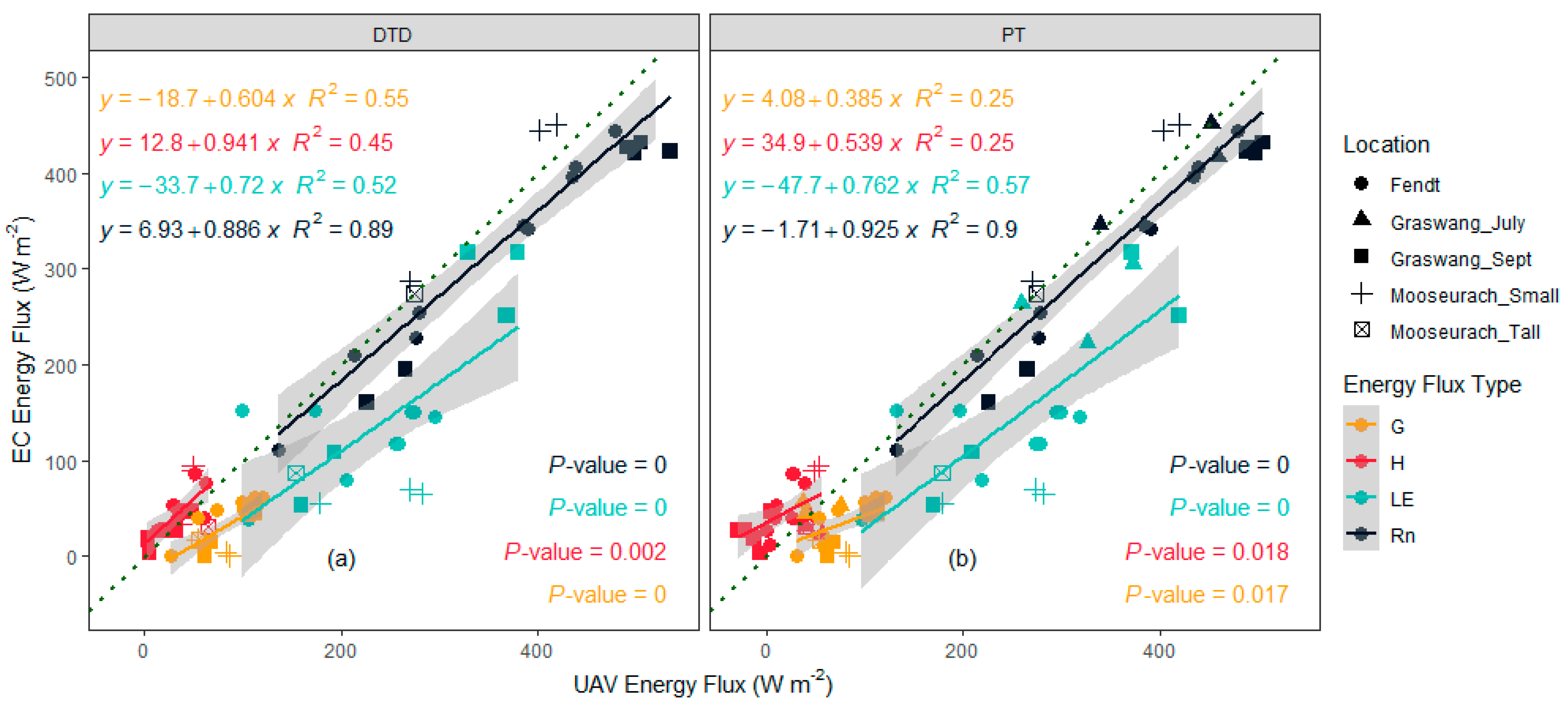
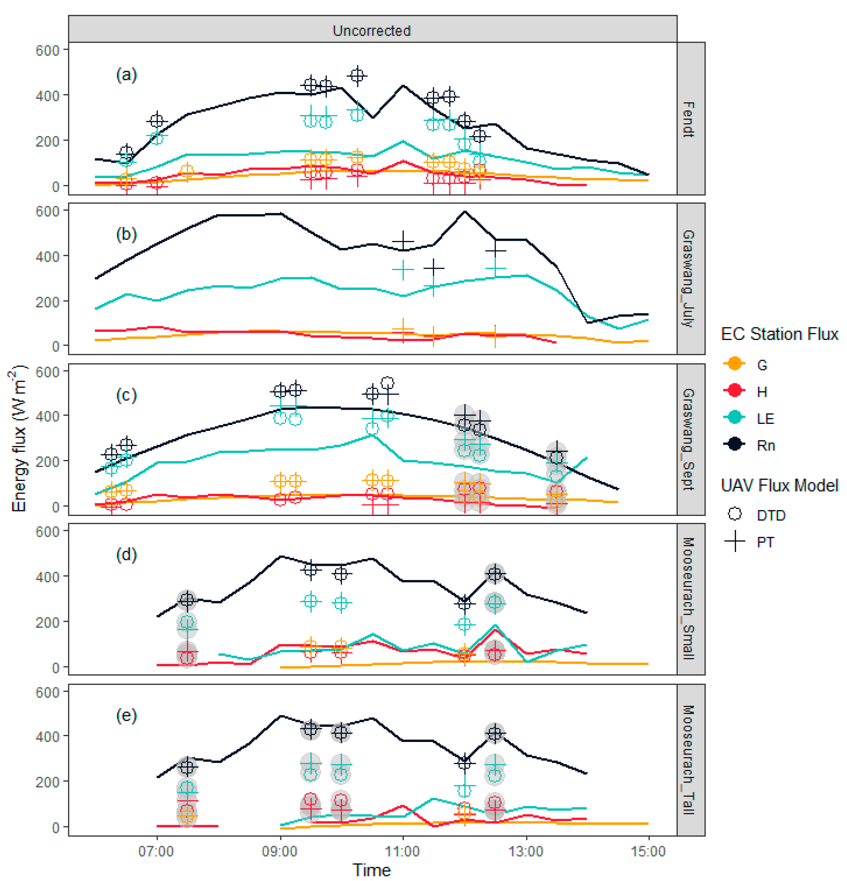
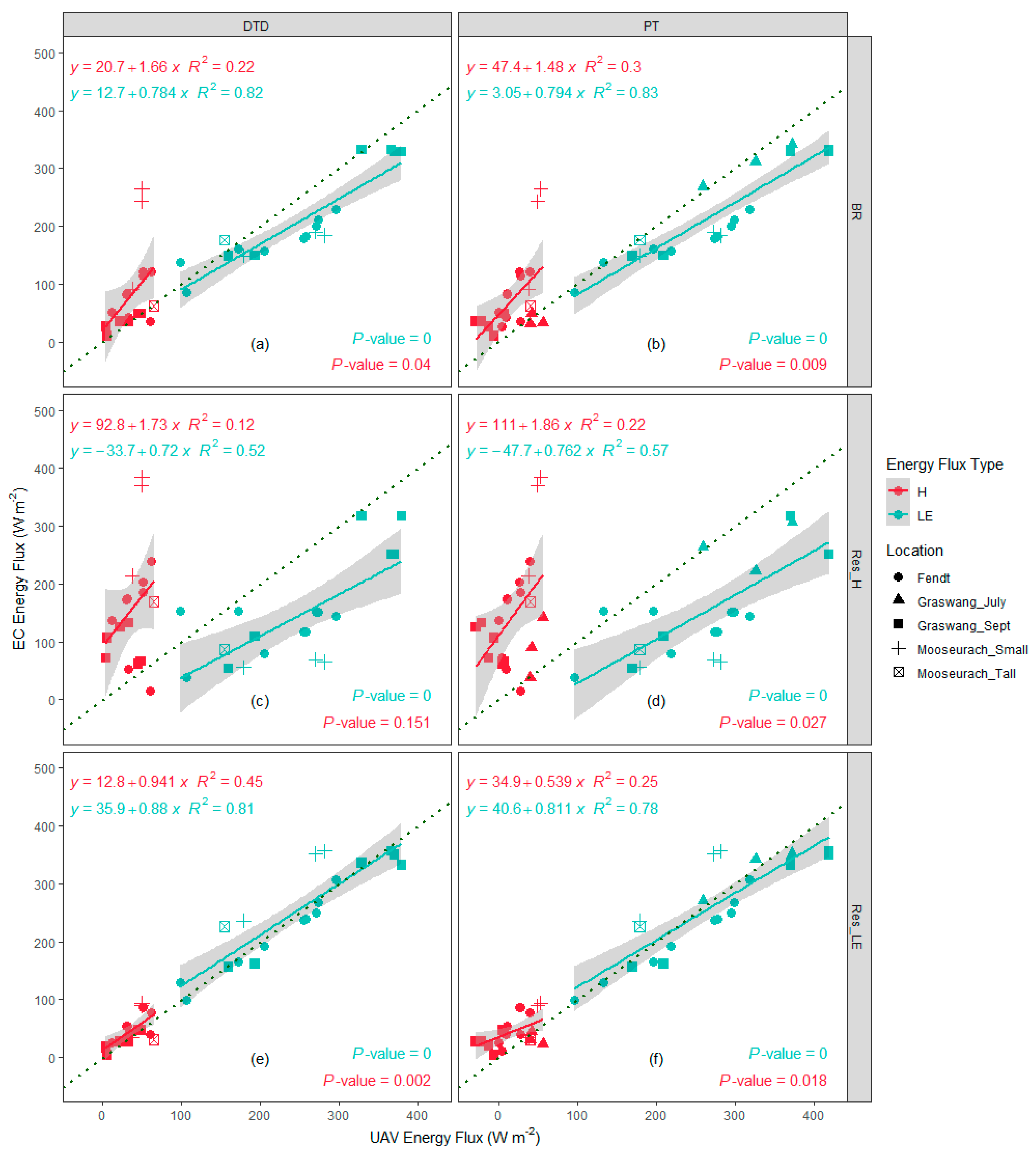
3.2. UAS vs. EC Station Flux Estimates

In total 22 UAS-EC comparisons are made, as eight 30 min EC flux estimates were flagged as low quality due to uncertainties in flux estimates, or footprint estimates, and were not suitable for comparison. We tested two variants of the Two Source Energy Balance model, TSEB-PT (Priestley Taylor) and TSEB-DTD (Dual Time Difference). Firstly we compare uncorrected EC station fluxes with TSEB outputs, and secondly corrected EC fluxes using three different methods to close the energy balance, namely by;

• adding imbalance residuals (Imb) to H (Res_H) and using uncorrected LE;
• adding imbalance residuals (Imb) to LE (Res_LE) and using uncorrected H;
• by maintaining the Bowen Ratio (BR);

We principally use the study-specific conversion factor from Section 3.1 to produce radiometric temperature inputs for TSEB (in K), but also show resultant TSEB outputs using the standard conversion factor (Equation (9)), and compare these to the EC control flux estimates.

When assessing the performance of the UAS vs. EC flux estimates, we consider the overall error using RMSE (<50 W m⁻² is considered ideal [70]) calculated, the mean bias (which can be corrected), the standard deviation (indicating the random error), and the regression coefficients which signal the predictive strength of the relationship (a slope of 1 indicates a 1:1 scaling relationship, and R² reflects the magnitude of the residuals compared to the regression line). The UAS and EC data are treated as “predicted” vs. “observed” respectively, and are plotted on the X and Y axes in regression plots accordingly [71]. We provide further analysis by examining fluxes from individual flights against EC flux time series.

The Trinity-Altum UAS produced very high quality thermal orthomosaics of our survey areas, with little blurring and very few artefacts, even in turbulent or gusty conditions. The TSEB outputs are also high-quality, an example of which can be seen in Figure 4, and in Appendix A Figure A1 and Figure A2.

TSEB-PT estimates of Rn_UAS were in closer agreement with Rn_EC than the DTD methods, with RMSE <50 W m⁻² across all sites (

Table 5. Statistics describing the relationship two TSEB models and uncorrected EC flux estimates.

Flux	Model	Location with Highest Errors	RMSE	Mean Bias	Standard Deviation
			(W m−2)
Rn	DTD	Graswang	53.0	35.2	40.8
H		Mooseurach	23.1	−10.8	21.0
LE		Mooseurach	121.6	103.7	65.2
G		Mooseurach	56.3	53.5	17.9
Rn	PT	Graswang	44.9	29.4	34.7
H		Mooseurach	36.1	−26.2	25.4
LE		Mooseurach	128.1	112.0	63.6
G		Mooseurach	51.6	45.1	25.7

, Figure 5). The DTD method aims to reduce biases in H and G caused by errors in remote sensing of T_rad (e.g., atmospheric transmission and/or inconsistencies in emissivity), and here DTD did provide more accurate and precise estimates of H_UAS than PT. While the G_EC-G_UAS correlation was closer to unity (slope = 0.60 vs. 0.39) using the DTD method, errors were still quite high (>50 W m⁻²) owing to the larger bias. The DTD method was more successful in reducing biases in H_UAS than G_UAS. This was also observed when we used the lower-accuracy T_rad inputs (using Equation (9)) for TSEB; both H_UAS and G_UAS from the DTD model had improved slopes, R², and significant P-values compared to PT model outputs (Figure A3, errors are reported in Table A1). LE_UAS and uncorrected LE_EC are not comparable (Figure 5), which reflects the differences in energy balance closure between EC and UAS-based methods where TSEB forces closure by adding imbalance residuals to LE_UAS.

Both TSEB models produced estimates of Rn_UAS in close agreement with Rn_EC throughout the day, with a tendency to over/underestimate in grassland/woodland regrowth sites (Fendt and Graswang/Mooseurach) (Figure 6). Diurnal changes in Rn_EC are closely matched by Rn_UAS with a maximum error of 111 W m⁻² at the Graswang site in September, which can be explained by the presence of cumulus clouds intermittently obscuring the sun after midday. This confirms an operational limitation in the UAS technique, whereby homogenous cloud cover is more likely to yield flux estimates which are consistent with EC station measurements, and is in agreement with [19].

G_UAS was consistently higher than G_EC and agreement is considered poor because the errors across all sites and times were high (RMSE > 50 W m⁻²). It should be noted that G_EC is measured at the EC station site only within a radius of ca. 5 m (i.e., not estimated for the wider area within the EC station footprint) [12], and therefore spatially distributed G_UAS are less comparable than other fluxes, especially where there is a difference in land cover across the survey site (e.g., grass vs. mowed grass). We investigated whether extracting the TSEB estimates of G from within a 5 m buffer of the EC station (compared to the EC station footprint) yields better agreement with EC station estimates (Figure A4), however there was no significant difference between G estimates (using the 5 m buffer vs. EC footprint) for both the DTD (t = 0.88, degrees of freedom = 40.66, p-value = 0.39) and PT (t = 0.97, d.f. = 49.43, p-value = 0.34) TSEB methods. The RMSE was actually higher when using the 5 m buffer to extract G rather than the EC footprint for both DTD (RMSE = 61.3 vs. 52.3) and PT (RMSE = 60.2 vs. 51.8). For both TSEB models, the greatest errors were observed at Graswang in September and July. These results highlight a potential weakness in TSEB, where G is estimated as a function of Rns, indicating further work is required comparing G_UAS and G_EC in different meteorological and environmental conditions. G_EC estimates in this study should be treated with caution as the in-situ soil measurements used to estimate G_EC may not be high-quality.

The best correlation between UAS and corrected EC flux estimates was from the Res_LE method of closing the surface energy balance (whereby all imbalance residuals are assigned to LE, and uncorrected H is used) (

Table 6. Statistics describing the relationship between different combinations of two TSEB model and three EC energy balance closure methods. Combined RMSE combines the errors for both LE and H fluxes.

Flux	EC Correction Type	Model	Location with Highest Errors	RMSE	Combined RMSE	Mean Bias	Standard Deviation
				(W m−2)
H	BR	DTD	Mooseurach	77.4	75.5	−46.1	64.0
LE			Mooseurach	73.1		−62.8	38.4
H	BR	PT	Mooseurach	79.0	71.9	−56.4	56.6
LE			Fendt	64.0		52.7	37.1
H	Res_H	DTD	Mooseurach	153.9	138.7	−122.0	96.6
LE			Mooseurach	121.6		103.7	65.2
H	Res_H	PT	Mooseurach	153.7	141.5	−127.7	25.4
LE			Fendt	128.1		112.0	63.6
H	Res_LE	DTD	Graswang	23.1	31.9	−10.8	21.0
LE			Mooseurach	38.7		−7.5	39.0
H	Res_LE	PT	Fendt	36.1	39.5	−26.2	25.4
LE			Mooseurach	42.6		10.5	42.3

). As TSEB explicitly calculates H_UAS, this an encouraging result, particularly for TSEB-DTD, RMSE, standard deviation and mean bias were all low, with a slight tendency for underestimated LE_UAS and H_UAS compared to EC data. Although the spread of the data were similar (both methods had R² ≈ 0.8), the regression coefficients were closer to unity using the DTD method (Figure 7). This finding is in agreement with [72] who compared EC estimates with lysimeters at an alpine grassland site (similar to Graswang), but in contrast to [20] who found closer UAS-EC agreement using the BR method at the Fendt site used in this study. Using the BR energy balance closure method, both DTD and PT methods estimated H poorly, but RMSE, accuracy and precision were all similar. The Res_H method of energy balance closure yielded the worst agreements between EC and UAS datasets, most likely because TSEB explicitly estimates H using the temperature gradient between Ta and Tc/Ts (as derived from T_rad) [7]. When errors in T_rad were introduced to the TSEB models (using Equation (9)), the UAS-EC correlations become highly insignificant using the PT method, however some improvements are observed in LE using the DTD method (Figure A5, Table A2). It should be noted here that the larger errors in radiometric temperature erroneously shift the energy fluxes from a LE- to a H-dominated system because Ts and Tc become hotter than Ta.

Figure 8 shows how UAS and corrected EC flux estimates vary at different sites across the day. For the two grassland sites (Graswang_Sept and Fendt) both LE_UAS and LE_EC, and H_UAS and H_EC agree very closely, especially when Res_LE method is used to close the EC energy balance. The agreement at Mooseurach is worse for the Res_LE method (with large under/overestimates of LE/H) than the BR method. The atmospheric conditions were stable on the day of the survey, leading to a number of low-quality flux readings from the EC stations. However, on aggregate using all data (including low quality flux data) the mean LE_UAS values for the small and tall tower footprints (233 and 231 W m⁻²) were similar to the mean LE_EC values using the BR closure method (219 and 255 W m⁻²). There are a number of possible explanations for poor agreement at Mooseurach, firstly atmospheric stability suppresses turbulent fluxes and can cause errors both in EC and TSEB estimates [33,48]. Secondly, on the day of the survey the average difference between air and surface temperature was 0.4 K; as the temperature gradient between the air and Ts and Tc drive the sensible heat flux, errors are more likely when this differential is low [7]. Thirdly, at this time of the year many of the shrubs and trees were losing their leaves, while we made every effort to measure LAI using the LICOR LAI 2200 plant canopy analyser, we had to manually adjust the LAI to account for biases caused by the lack of green leaves [73]. As TSEB is very sensitive to LAI, this could be a significant source of error [23,74]. Fourthly, the site was water-logged, which may be problematic for TSEB because the model has not been tested in water-logged or flooded conditions, therefore the assumed relationship between Rns and G may not apply here, which may increase errors in G estimates. Lastly, the vegetation structure is very complex at this site which may increase the influence of processes which are not accounted for in either TSEB or EC station estimates/measurements (including canopy heat storage, biochemical canopy storage, and horizontal advection [35]), and further surveys under a variety of plant growth and meteorological conditions would help understand the capabilities of this UAS for flux mapping in heterogeneous vegetated areas. Despite the low sample size in Mooseurach, we include these data in the ensemble to demonstrate how site surveys with completely different vegetation and meteorological characteristics can be compared using the equipment and same methodology.

The findings of this paper highlight an important limitation in comparing UAS and EC flux estimates. Both TSEB models force energy balance closure by assigning all residuals (after G and H have been calculated) to LE, whereas the EC station balance is rarely closed, and so requires a closure method to allow comparability with UAS estimates. The literature has shown that the most accurate EC energy balance closure methods vary with different sites/site conditions [35]; EC vs. lysimeter comparisons show better performance in the Res_LE in an alpine grassland [72], whereas in different pre-alpine grasslands the BR method outperforms [52,75]. In previous remote sensing-EC comparisons, both methods have also been adopted (see [76,77] for Res_LE, and [19,22] for BR methods. Here we show that Res_LE produces consistently lower errors across all sites than BR (

Table 7. Site level error statistics for the two TSEB models, and the two most appropriate EC energy balance correction methods, Res_LE and BR.

Location	Model	BR		Res_LE
		RMSE	Mean Bias	RMSE	Mean Bias
		(W m−2)
Graswang	DTD	59.1	19.3	51.6	38.4
Fendt		48.6	−2.8	33.2	16.6
Mooseurach		97.4	−46.1	53.0	−11.7
All sites		75.3	−5.0	44.7	17.6
Graswang	PT	50.9	26.8	47.4	24.9
Fendt		56.6	−19.9	37.8	16
Mooseurach		87.2	−7.9	49.5	−11.4
All sites		71.9	17.7	44.2	14.7

), owing to a better regression slope (closer to 1) for both H and LE (Figure 7e,f versus a and b). This result could be expected given that this EC energy balance closure method mirrors that of TSEB, but perhaps the conclusion to be drawn is that while the EC station method is a robust control method because it directly measures fluxes and reports uncertainty (usually in the form of a quality control flag, and or percentage uncertainty), the EC energy balance closure method itself is subject to uncertainty, and therefore the EC-UAS agreements should be treated cautiously.

Both TSEB methods yielded low errors in conjunction with Res_LE (Table 6) and there was no significant difference in residuals for LE and H between DTD and LE (Welch Two Sample t-test; t = −0.009, d.f. = 237.84, p-value = 0.99). However, the regression coefficients were more favorable for both LE and H using the DTD method (Figure 7). These slight benefits in using DTD show that it may not be worth the additional logistical challenges involved in collecting the data for DTD, whereby a UAS survey must be conducted shortly after sunrise [18], however further work (at more sites, under a range of conditions) is necessary to support this.

While the EC stations report measurement uncertainty, the TSEB methodology does not. This study produces error statistics for TSEB flux estimates that could be used as a foundation to quantify uncertainty and error propagation in future UAS-derived estimates, which may be important if the TSEB is used to bridge the scale gap between EC- and satellite-based measurements.

A clear path for further work is to collect more data using this UAS at non-grassland sites. Grassland sites are ideal systems for testing the UAS because the vegetation communities are simple, access is easy and flights can be conducted safely with a low risk of striking obstacles. We found that the errors were higher at the more complex regrowth woodland site (Mooseurach) compared to the grassland sites, however given the small sample size and EC quality control flags, it is unclear as to whether these errors are caused by the vegetation complexity, the non-ideal stable meteorological conditions [78], or instrumentation errors. Further surveys at this site at more active times of the year (e.g., high summer) would enable further inter-site comparison, and a more robust test of the UAS. The network of ICOS EC stations is distributed over many different land cover types, and given the long range of the UAS, many more EC-UAS comparisons could be made.

Converting from DN to radiometric temperature using our empirical method resulted in a 19% reduction in RMSE across all fluxes (and 20%, 28%, 17%, and 15% reductions for Rn, H, LE and G respectively), compared to the standard conversion factor. While we made important steps in correcting radiometric bias in the thermal infrared data, further improvements could be made by performing radiometric calibration using a black body reference source [29]. However, the method employed in this paper shows that reasonable environmental and atmospheric corrections can be applied without the use of a blackbody reference source in a controlled environment.

The UAS used in this study has the added benefits of providing spatially distributed estimates at very high resolution. This can enable researchers to discern how differences in vegetation types (e.g., forest vs. shrub vs. grass), phenotypes (of cropped systems), and land use practices (e.g., the use of different fertilisers) can influence the surface energy balance (and water usage). The system could be used as a low-cost complement to the EC station and can help resolve small-scale variability within the modelled footprint, however it is worth noting that the EC station methods are better suited to long term measurements, rather than mapping instantaneous fluxes. Given the flexibility and long range of the UAS, it can also be used to bridge the scale gap between EC station and satellite-derived fluxes and/or for precision agriculture practices.

4. Conclusions

This study has successfully demonstrated the application of an off-the-shelf unmanned aerial system (e.g., Trinity F90+ and Micasense Altum) for reproducing eddy covariance station-derived energy flux estimates using the Two-Source Energy Balance Model. Utilising the long flight time and range of the UAS, we demonstrate the potential for these systems to be used to spatially map fluxes over heterogeneous land use/cover types. Comparisons of UAS- and eddy covariance- (industry standard) derived flux estimates, indicated good agreement between the two methodologies with errors <50 W m⁻² for Rn, LE and H. Furthermore, the UAS method provides new and additional spatial information to EC flux estimates. We also demonstrate the importance of proper and appropriate UAS thermal sensor calibration, and its impact on derived fluxes estimates; specifically achieving 19% improvement in accuracies using a simple field-based calibration step.

Areas for future work should include increasing the range and diversity of land cover types; as well as the potential for upscaling this work from EC and UAS to satellite derived flux estimates. In addition, given the low errors in LE estimates, it could be further adapted to high-resolution evapotranspiration mapping, particularly in water-scarce agricultural settings which rely on irrigation.

References

1. Duveiller, G.; Hooker, J.; Cescatti, A. The mark of vegetation change on Earth’s surface energy balance. Nat. Commun. 2018, 9, 1–12. [Google Scholar] [CrossRef] [Green Version]
2. Lawrence, P.J.; Chase, T.N. Investigating the climate impacts of global land cover change in the community climate system model. Int. J. Climatol. 2010, 30, 2066–2087. [Google Scholar] [CrossRef]
3. Shukla, J.; Mintz, Y.; Guo, Z.; Bonan, G.; Chan, E.; Cox, P.; Gordon, C.T.; Kanae, S.; Kowalczyk, E.; Lawrence, D.; et al. Influence of Land-Surface Evapotranspiration on the Earth’s Climate. Science 1982, 215, 1498–1501. [Google Scholar] [CrossRef] [PubMed]
4. Bonan, G.B. Forests and Climate Change: Forcings, Feedbacks, and the Climate Benefits of Forests. Science 2008, 320, 1444–1449. [Google Scholar] [CrossRef] [PubMed] [Green Version]
5. Perugini, L.; Caporaso, L.; Marconi, S.; Cescatti, A.; Quesada, B.; de Noblet-Ducoudré, N.; House, J.I.; Arneth, A. Biophysical effects on temperature and precipitation due to land cover change. Environ. Res. Lett. 2017, 12, 053002. [Google Scholar] [CrossRef]
6. Spracklen, D.V.; Baker, J.C.A.; Garcia-Carreras, L.; Marsham, J.H. The Effects of Tropical Vegetation on Rainfall. Annu. Rev. Environ. Resour. 2018, 43, 193–218. [Google Scholar] [CrossRef]
7. Norman, J.M.; Kustas, W.P.; Humes, K.S. Source approach for estimating soil and vegetation energy fluxes in observations of directional radiometric surface temperature. Agric. For. Meteorol. 1995, 77, 263–293. [Google Scholar] [CrossRef]
8. Quattrochi, D.A.; Luvall, J.C. Thermal infrared remote sensing for analysis of landscape ecological processes: Methods and applications. Landsc. Ecol. 1999, 14, 577–598. [Google Scholar] [CrossRef]
9. Lin, B.B. Agroforestry management as an adaptive strategy against potential microclimate extremes in coffee agriculture. Agric. For. Meteorol. 2007, 144, 85–94. [Google Scholar] [CrossRef]
10. Lawrence, D.; Vandecar, K. Effects of tropical deforestation on climate and agriculture. Nat. Clim. Chang. 2015, 5, 27–36. [Google Scholar] [CrossRef]
11. Liang, S.; Wang, J. Advanced Remote Sensing: Terrestrial Information Extraction and Applications; Elsevier: Amsterdam, The Netherlands, 2019; ISBN 9780128158265. [Google Scholar]
12. Kiese, R.; Fersch, B.; Baessler, C.; Brosy, C.; Butterbach-Bahl, K.; Chwala, C.; Dannenmann, M.; Fu, J.; Gasche, R.; Grote, R.; et al. The TERENO pre-alpine observatory: Integrating meteorological, hydrological, and biogeochemical measurements and modeling. Vadose Zone J. 2018, 17, 1–17. [Google Scholar] [CrossRef]
13. Rebmann, C.; Aubinet, M.; Schmid, H.; Arriga, N.; Aurela, M.; Burba, G.; Clement, R.; De Ligne, A.; Fratini, G.; Gielen, B.; et al. ICOS eddy covariance flux-station site setup: A review. Int. Agrophysics 2018, 32, 471–494. [Google Scholar] [CrossRef]
14. Allen, R.G.; Tasumi, M.; Morse, A.; Trezza, R.; Wright, J.L.; Bastiaanssen, W.; Kramber, W.; Lorite, I.; Robison, C.W. Satellite-Based Energy Balance for Mapping Evapotranspiration with Internalized Calibration (METRIC)—Applications. J. Irrig. Drain. Eng. 2007, 133, 395–406. [Google Scholar] [CrossRef]
15. Reis, T.G.; Monteiro, R.O.C.; Albuquerque, M.G.; Espinoza, J.M.A.; Ferreira, J.A.C.; Moreria, E.G. Actual Evapotranspiration Estimated By Orbital Sensors, Uav and Meteorological Station for Vineyards in the Southern Brazil. In Proceedings of the IV Inovagri International Meeting, Fortaleza, Brazil, 2–6 October 2017. [Google Scholar]
16. Hoffmann, H.; Nieto, H.; Jensen, R.; Guzinski, R.; Zarco-Tejada, P.; Friborg, T. Estimating evaporation with thermal UAV data and two-source energy balance models. Hydrol. Earth Syst. Sci. 2016, 20, 697–713. [Google Scholar] [CrossRef] [Green Version]
17. Guzinski, R.; Nieto, H.; Jensen, R.; Mendiguren, G. Remotely sensed land-surface energy fluxes at sub-field scale in heterogeneous agricultural landscape and coniferous plantation. Biogeosciences 2014, 11, 5021–5046. [Google Scholar] [CrossRef] [Green Version]
18. Nieto, H.; Kustas, W.P.; Torres-rúa, A.; Alfieri, J.G.; Gao, F.; Anderson, M.C.; Alex, W.; Song, L. Evaluation of TSEB turbulent fluxes using different methods for the retrieval of soil and canopy component temperatures from UAV thermal and multispectral imagery. Irrig. Sci. 2019, 37, 389–406. [Google Scholar] [CrossRef] [Green Version]
19. Brenner, C.; Zeeman, M.; Bernhardt, M.; Schulz, K. Estimation of evapotranspiration of temperate grassland based on high-resolution thermal and visible range imagery from unmanned aerial systems. Int. J. Remote Sens. 2018, 39, 5141–5174. [Google Scholar] [CrossRef] [Green Version]
20. Brenner, C.; Thiem, C.E.; Wizemann, H.-D.; Bernhardt, M.; Schulz, K. Estimating spatially distributed turbulent heat fluxes from high-resolution thermal imagery acquired with a UAV system. Int. J. Remote Sens. 2017, 38, 3003–3026. [Google Scholar] [CrossRef] [Green Version]
21. Niu, H.; Zhao, T.; Wang, D.; Chen, Y. Evapotranspiration Estimation with UAVs in Agriculture: A Review. Preprints 2019. [Google Scholar] [CrossRef]
22. Andreu, A.; Dube, T.; Nieto, H.; Mudau, A.E.; González-Dugo, M.P.; Guzinski, R.; Hülsmann, S. Remote sensing of water use and water stress in the African savanna ecosystem at local scale – Development and validation of a monitoring tool. Phys. Chem. Earth 2019. [Google Scholar] [CrossRef]
23. Burchard-Levine, V.; Nieto, H.; Riaño, D.; Migliavacca, M.; El-Madany, T.S.; Perez-Priego, O.; Carrara, A.; Martín, M.P. Seasonal adaptation of the thermal-based two-source energy balance model for estimating evapotranspiration in a semiarid tree-grass ecosystem. Remote Sens. 2020, 12, 904. [Google Scholar] [CrossRef] [Green Version]
24. Xia, T.; Kustas, W.P.; Anderson, M.C.; Alfieri, J.G.; Gao, F.; McKee, L.; Prueger, J.H.; Geli, H.M.E.; Neale, C.M.U.; Sanchez, L.; et al. Mapping evapotranspiration with high-resolution aircraft imagery over vineyards using one-and two-source modeling schemes. Hydrol. Earth Syst. Sci. 2016, 20. [Google Scholar] [CrossRef] [Green Version]
25. Alhassan, A.; Jin, M. Evapotranspiration in the Tono Reservoir Catchment in Upper East Region of Ghana Estimated by a Novel TSEB Approach from ASTER Imagery. Remote Sens. 2020, 12, 569. [Google Scholar] [CrossRef] [Green Version]
26. Chávez, J.L.; Gowda, P.H.; Howell, T.A.; Neale, C.M.U.; Copeland, K.S. Estimating hourly crop ET using a two-source energy balance model and multispectral airborne imagery. Irrig. Sci. 2009, 28, 79–91. [Google Scholar] [CrossRef]
27. Kafle, H.K.; Yamaguchi, Y. Effects of topography on the spatial distribution of evapotranspiration over a complex terrain using two-source energy balance model with ASTER data. Hydrol. Process. 2009, 23, 2295–2306. [Google Scholar] [CrossRef]
28. Torres-Rua, A. Vicarious Calibration of sUAS Microbolometer Temperature Imagery for Estimation of Radiometric Land Surface Temperature. Sensors 2017, 17, 1499. [Google Scholar] [CrossRef] [PubMed] [Green Version]
29. Weslien, P.; Klemedtsson, L.; Eklundh, L.; Kelly, J.; Kljun, N.; Olsson, P.O.; Mihai, L.; Liljeblad, B.; Weslien, P.; Klemedtsson, L.; et al. Challenges and best practices for deriving temperature data from an uncalibrated UAV thermal infrared camera. Remote Sens. 2019, 11, 567. [Google Scholar] [CrossRef] [Green Version]
30. Sagan, V.; Maimaitijiang, M.; Sidike, P.; Eblimit, K.; Peterson, K.; Hartling, S.; Esposito, F.; Khanal, K.; Newcomb, M.; Pauli, D.; et al. UAV-Based High Resolution Thermal Imaging for Vegetation Monitoring, and Plant Phenotyping Using ICI 8640 P, FLIR Vue Pro R 640, and thermoMap Cameras. Remote Sens. 2019, 11, 330. [Google Scholar] [CrossRef] [Green Version]
31. Guzinski, R.; Nieto, H.; Sandholt, I.; Karamitilios, G. Modelling high-resolution actual evapotranspiration through Sentinel-2 and Sentinel-3 data fusion. Remote Sens. 2020, 12, 1433. [Google Scholar] [CrossRef]
32. He, R.; Jin, Y.; Kandelous, M.M.; Zaccaria, D.; Sanden, B.L.; Snyder, R.L.; Jiang, J.; Hopmans, J.W. Evapotranspiration estimate over an almond orchard using Landsat satellite observations. Remote Sens. 2017, 9, 436. [Google Scholar] [CrossRef] [Green Version]
33. Alfieri, J.G.; Kustas, W.P.; Nieto, H.; Prueger, J.H.; Hipps, L.E.; McKee, L.G.; Gao, F.; Los, S. Influence of wind direction on the surface roughness of vineyards. Irrig. Sci. 2019, 37, 359–373. [Google Scholar] [CrossRef]
34. Kormann, R.; Meixner, F.X. An analytical footprint model for non-neutral stratification. Boundary-Layer Meteorol. 2001, 99, 207–224. [Google Scholar] [CrossRef]
35. Mauder, M.; Foken, T.; Cuxart, J. Surface-Energy-Balance Closure over Land: A Review. Boundary-Layer Meteorol. 2020, 177, 395–426. [Google Scholar] [CrossRef]
36. Morillas, L.; García, M.; Nieto, H.; Villagarcia, L.; Sandholt, I.; Gonzalez-Dugo, M.P.; Zarco-Tejada, P.J.; Domingo, F. Using radiometric surface temperature for surface energy flux estimation in Mediterranean drylands from a two-source perspective. Remote Sens. Environ. 2013, 136, 234–246. [Google Scholar] [CrossRef] [Green Version]
37. Tilahun, T. High-Resolution Mapping of Subsurface Tile Drainage in Agricultural Fields Using an Unmanned Aerial System (UAS). Univ. Res. Symp. 2019. [Google Scholar] [CrossRef]
38. Hutton, J.J.; Lipa, G.; Baustian, D.; Sulik, J.; Bruce, R.W. High Accuracy Direct Georeferencing of the Altum Multispectral UAV Camera and its Application to High Throughput Plant Phenotyping. Int. Arch. Photogramm. Remote Sens. Spat. Inf. Sci. 2020. [Google Scholar] [CrossRef]
39. Honkavaara, E.; Näsi, R.; Oliveira, R.; Viljanen, N.; Suomalainen, J.; Khoramshahi, E.; Hakala, T.; Nevalainen, O.; Markelin, L.; Vuorinen, M.; et al. Using multitemporal hyper-and multispectral UAV imaging for detecting bark beetle infestation on norway spruce. Int. Arch. Photogramm. Remote Sens. Spat. Inf. Sci. 2020, 43, 429–434. [Google Scholar] [CrossRef]
40. Miller, I.J.; Schieber, B.; De Bey, Z.; Benner, E.; Ortiz, J.D.; Girdner, J.; Patel, P.; Coradazzi, D.G.; Henriques, J.; Forsyth, J. Analyzing crop health in vineyards through a multispectral imaging and drone system. In Proceedings of the 2020 Systems and Information Engineering Design Symposium, SIEDS, Charlottesville, VA, USA, 24–24 April 2020. [Google Scholar]
41. ICOS-Deutschland ICOS: Graswang (C3). Available online: https://www.icos-infrastruktur.de/en/icos-d/komponenten/oekosysteme/beobachtungsstandorte/graswang-c3/ (accessed on 18 January 2021).
42. ICOS-Deutschland ICOS: Fendt (C1). Available online: https://www.icos-infrastruktur.de/en/icos-d/komponenten/oekosysteme/beobachtungsstandorte/fendt-c1/ (accessed on 18 January 2021).
43. ICOS-Deutschland ICOS: Mooseurach (C3). Available online: https://www.icos-infrastruktur.de/en/icos-d/komponenten/oekosysteme/beobachtungsstandorte/mooseurach-c3/ (accessed on 18 January 2021).
44. Hommeltenberg, J.; Schmid, H.P.; Drösler, M.; Werle, P. Can a bog drained for forestry be a stronger carbon sink than a natural bog forest? Biogeosciences 2014, 11, 3477–3493. [Google Scholar] [CrossRef] [Green Version]
45. Fratini, G.; Mauder, M. Towards a consistent eddy-covariance processing: An intercomparison of EddyPro and TK3. Atmos. Meas. Tech. 2014, 7, 2273–2281. [Google Scholar] [CrossRef] [Green Version]
46. Foken, T.; Aubinet, M.; Leuning, R. The Eddy Covariance Method. In Eddy Covariance; Springer: Berlin/Heidelberg, Germany, 2012; pp. 1–19. [Google Scholar]
47. Mauder, M.; Cuntz, M.; Drüe, C.; Graf, A.; Rebmann, C.; Schmid, H.P.; Schmidt, M.; Steinbrecher, R. A strategy for quality and uncertainty assessment of long-term eddy-covariance measurements. Agric. For. Meteorol. 2013, 169, 122–135. [Google Scholar] [CrossRef]
48. Heidbach, K.; Schmid, H.P.; Mauder, M. Experimental evaluation of flux footprint models. Agric. For. Meteorol. 2017, 246, 142–153. [Google Scholar] [CrossRef] [Green Version]
49. Kljun, N.; Calanca, P.; Rotach, M.W.; Schmid, H.P. A simple two-dimensional parameterisation for Flux Footprint Prediction (FFP). Geosci. Model Dev. 2015, 8, 3695–3713. [Google Scholar] [CrossRef] [Green Version]
50. Templeton, R.C.; Vivoni, E.R.; Méndez-Barroso, L.A.; Pierini, N.A.; Anderson, C.A.; Rango, A.; Laliberte, A.S.; Scott, R.L. High-resolution characterization of a semiarid watershed: Implications on evapotranspiration estimates. J. Hydrol. 2014, 509, 306–319. [Google Scholar] [CrossRef]
51. Foken, T. The energy balance closure problem: An overview. Ecol. Appl. 2008, 18, 1351–1367. [Google Scholar] [CrossRef] [PubMed]
52. Mauder, M.; Genzel, S.; Fu, J.; Kiese, R.; Soltani, M.; Steinbrecher, R.; Zeeman, M.; Banerjee, T.; De Roo, F.; Kunstmann, H. Evaluation of energy balance closure adjustment methods by independent evapotranspiration estimates from lysimeters and hydrological simulations. Hydrol. Process. 2018, 32, 39–50. [Google Scholar] [CrossRef]
53. Shuttleworth, W.J.; Wallace, J.S. Evaporation from sparse crops-an energy combination theory. Q. J. R. Meteorol. Soc. 1985, 111, 839–855. [Google Scholar] [CrossRef]
54. Priestley, C.H.B.; Taylor, R.J. On the Assessment of Surface Heat Flux and Evaporation Using Large-Scale Parameters. Mon. Weather Rev. 1972, 100, 81–92. [Google Scholar] [CrossRef]
55. Bellvert, J.; Jofre-Ĉekalović, C.; Pelechá, A.; Mata, M.; Nieto, H. Feasibility of Using the Two-Source Energy Balance Model (TSEB) with Sentinel-2 and Sentinel-3 Images to Analyze the Spatio-Temporal Variability of Vine Water Status in a Vineyard. Remote Sens. 2020, 12, 2299. [Google Scholar] [CrossRef]
56. Colaizzi, P.; Kustas, W.P.; Anderson, M.C. Two-source energy balance model estimates of evapotranspiration using component and composite surface temperatures. Adv. Water Resour. 2012, 50, 134–151. [Google Scholar] [CrossRef] [Green Version]
57. Kustas, W.; Anderson, M. Advances in thermal infrared remote sensing for land surface modeling. Agric. For. Meteorol. 2009, 149, 2071–2081. [Google Scholar] [CrossRef]
58. Wind Energy Data for Switzerland. Available online: https://wind-data.ch/tools/profile.php?h=3.25&v=2.17&z0=0.2&abfrage=Aktualisieren (accessed on 5 January 2021).
59. FLIR Tech Note: Radiometric Temperature Measurements. Available online: https://www.flir.com/globalassets/guidebooks/suas-radiometric-tech-note-en.pdf (accessed on 7 May 2020).
60. Schmugge, T.; French, A.; Ritchie, J.C.; Rango, A.; Pelgrum, H. Temperature and emissivity separation from multispectral thermal infrared observations. Remote Sens. Environ. 2002, 79, 189–198. [Google Scholar] [CrossRef]
61. Nolan, R.; Padilla-Parra, S. ijtiff: An R package providing TIFF I/O for ImageJ users. J. Open Source Softw. 2018, 3, 633. [Google Scholar] [CrossRef] [Green Version]
62. RStudio Team RStudio: Integrated Development for R.; RStudio, Inc.: Boston, MA, USA, 2016; Volume 42, p. 14.
63. CloudCompare 3D Point Cloud and Mesh Processing Software; 2021. Available online: https://www.danielgm.net/cc/ (accessed on 13 November 2020).
64. Isenburg, M. LAStools—Efficient LiDAR Processing Software; 2011. Available online: https://rapidlasso.com/lastools/ (accessed on 20 November 2020).
65. Roussel, J.-R.; Auty, D.; Coops, N.C.; Tompalski, P.; Goodbody, T.R.H.; Meador, A.S.; Bourdon, J.-F.; de Boissieu, F.; Achim, A. lidR: An R package for analysis of Airborne Laser Scanning (ALS) data. Remote Sens. Environ. 2020, 251, 112061. [Google Scholar] [CrossRef]
66. Pareeth, S.; Karimi, P.; Shafiei, M.; De Fraiture, C.; Pareeth, S.; Karimi, P.; Shafiei, M.; De Fraiture, C. Mapping Agricultural Landuse Patterns from Time Series of Landsat 8 Using Random Forest Based Hierarchial Approach. Remote Sens. 2019, 11, 601. [Google Scholar] [CrossRef] [Green Version]
67. Stefan, V. R—Using Random Forests, Support Vector Machines and Neural Networks for a Pixel Based Supervised Classification of Sentinel-2 Multispectral Images. Available online: https://valentinitnelav.github.io/satellite-image-classification-r/#visualize-classifications (accessed on 2 March 2021).
68. Byrne, K.A.; Kiely, G.; Leahy, P. CO2 fluxes in adjacent new and permanent temperate grasslands. Agric. For. Meteorol. 2005, 135, 82–92. [Google Scholar] [CrossRef]
69. Mauder, M.; Foken, T.; Clement, R.; Elbers, J.A.; Eugster, W.; Grünwald, T.; Heusinkveld, B.; Kolle, O. Quality control of CarboEurope flux data - Part 2: Inter-comparison of eddy-covariance software. Biogeosciences 2008, 5, 451–462. [Google Scholar] [CrossRef] [Green Version]
70. Kalma, J.D.; McVicar, T.R.; McCabe, M.F. Estimating Land Surface Evaporation: A Review of Methods Using Remotely Sensed Surface Temperature Data. Surv. Geophys. 2008, 29, 421–469. [Google Scholar] [CrossRef]
71. Piñeiro, G.; Perelman, S.; Guerschman, J.P.; Paruelo, J.M. How to evaluate models: Observed vs. predicted or predicted vs. observed? Ecol. Modell. 2008, 216, 316–322. [Google Scholar] [CrossRef]
72. Wohlfahrt, G.; Irschick, C.; Thalinger, B.; Hörtnagl, L.; Obojes, N.; Hammerle, A. Insights from Independent Evapotranspiration Estimates for Closing the Energy Balance: A Grassland Case Study. Vadose Zo. J. 2010, 9, 1025–1033. [Google Scholar] [CrossRef] [Green Version]
73. Calders, K.; Origo, N.; Disney, M.; Nightingale, J.; Woodgate, W.; Armston, J.; Lewis, P. Variability and bias in active and passive ground-based measurements of effective plant, wood and leaf area index. Agric. For. Meteorol. 2018, 252, 231–240. [Google Scholar] [CrossRef]
74. Kustas, W.P.; Alfieri, J.G.; Nieto, H.; Wilson, T.G.; Gao, F.; Anderson, M.C. Utility of the two-source energy balance (TSEB) model in vine and interrow flux partitioning over the growing season. Irrig. Sci. 2019, 37, 375–388. [Google Scholar] [CrossRef]
75. Hirschi, M.; Michel, D.; Lehner, I.; Seneviratne, S.I. A site-level comparison of lysimeter and eddy covariance flux measurements of evapotranspiration. Hydrol. Earth Syst. Sci 2017, 21, 1809–1825. [Google Scholar] [CrossRef] [Green Version]
76. Burchard-Levine, V.; Nieto, H.; Riaño, D.; Migliavacca, M.; El-Madany, T.S.; Perez-Priego, O.; Carrara, A.; Martín, M.P. Adapting the thermal-based two-source energy balance model to estimate energy fluxes in a complex tree-grass ecosystem. Hydrol. Earth Syst. Sci. Discuss. 2019, 1–37. [Google Scholar] [CrossRef] [Green Version]
77. Guzinski, R.; Nieto, H. Evaluating the feasibility of using Sentinel-2 and Sentinel-3 satellites for high-resolution evapotranspiration estimations. Remote Sens. Environ. 2019, 221, 157–172. [Google Scholar] [CrossRef]
78. Nieto, H.; Kustas, W.P.; Alfieri, J.G.; Gao, F.; Hipps, L.E.; Los, S.; Prueger, J.H.; McKee, L.G.; Anderson, M.C. Impact of different within-canopy wind attenuation formulations on modelling sensible heat flux using TSEB. Irrig. Sci. 2019, 37. [Google Scholar] [CrossRef]
Figure 1. Data collection and processing scheme for the production and assessment of spatially-distributed energy flux estimates from the Trinity-Altum UAS.
Remotesensing 13 01286 g001
Figure 2. Maps of the three EC station sites surveyed in this paper; there are two predominantly grassland sites (a) Fendt (20 ha) and (b) Graswang (23 ha), and (c) one forest regrowth site at Mooseurach (20 ha) which has two EC stations, one at 6 m tall (“Small”), and one at 30 m (“Tall”). The locations of the sites are shown in (d). Each map shows a representative land cover map of the site, with the land covers which are used in the TSEB model (Section 2.4.3), as well as some examples of the EC station footprints that were delineated in this study (Section 2.2.2).
Remotesensing 13 01286 g002
Figure 3. Relationship between digital number (DN) derived from the thermal infrared band from airborne Altum images and ground control data from the Apogee SI 220 infrared radiometer. The green dotted line represents the conversion factor published by Micasense (Equation (9)). The grey shaded area indicates standard error.
Remotesensing 13 01286 g003
Figure 4. TSEB-PT outputs for a survey in the afternoon of 17 September 2020 at Fendt, showing how the surface energy balance is dis-tributed across the site: Rn (a) and LE (c) are higher where the canopy surface is cooler (here where the grass is not cut), and H (b) and G (d) are higher where the grass has been mowed, and consequently the canopy and soil temperatures (Tc and Ts) are higher.
Remotesensing 13 01286 g004
Figure 5. Energy flux comparisons using uncorrected EC station (observed) and UAS-derived (modelled) data. Here two TSEB methods are tested, (a) Dual Time Difference (DTD) and (b) Priestly-Taylor (PT). Standard error is shaded in grey and linear regression coefficients are coloured to match their flux type. The green dotted line shows unity and p-values show the significance of the linear regressions.
Remotesensing 13 01286 g005
Figure 6. Time series plots of uncorrected Rn, H, LE and G from both the EC and UAS. The data were collected on (a) 17 September 2020, (b) 20 July 2020, (c) 15 September 2020 and (d,e) 20 October 2020. Grey points indicate where UAS-EC comparisons were not possible due to low quality EC-flux estimates.
Remotesensing 13 01286 g006
Figure 7. The relationship between UAV- and EC-derived (modelled vs. observed) energy fluxes using three methods to close the surface energy balance in EC data. (a,b) shows BR = maintaining the Bowen Ratio, (c,d) shows Res_H = attributing all residuals to H and maintaining uncorrected LE, and (e,f) Res_LE is the opposite of Res_H. Green dotted line represents unity and p-values show the significances of the linear regression (3 significant figures).
Remotesensing 13 01286 g007
Figure 8. Time series plots of corrected EC-derived H and LE fluxes (using methods BR, Res_H and Res_LE), with the instantaneous H and LE fluxes from two TSEB methods (DTD and PT) derived from UAS data displayed as points. The data are from (ac) Fendt on 17 September 2020, (df) Graswang on 20 July 2020, (gi) Graswang on 15 September 2020, (jl) the small EC tower at Mooseurach on 20 October 2020 and (mo) the tall EC tower on 20 October 2020. Grey points indicate where UAS-EC comparisons were not possible due to low quality EC-flux estimates, however they are shown here for completeness.
Remotesensing 13 01286 g008