Prediction of Forest Aboveground Biomass Using Multitemporal Multispectral Remote Sensing Data

Abstract

Forest aboveground biomass (AGB) is a prime forest parameter that requires global level estimates to study the global carbon cycle. Light detection and ranging (LiDAR) is the state-of-the-art technology for AGB prediction but it is expensive, and its coverage is restricted to small areas. On the contrary, spaceborne Earth observation data are effective and economical information sources to estimate and monitor AGB at a large scale. In this paper, we present a study on the use of different spaceborne multispectral remote sensing data for the prediction of forest AGB. The objective is to evaluate the effects of temporal, spectral, and spatial capacities of multispectral satellite data for AGB prediction. The study was performed on multispectral data acquired by Sentinel-2, RapidEye, and Dove satellites which are characterized by different spatial resolutions, temporal availability, and number of spectral bands. A systematic process of least absolute shrinkage and selection operator (lasso) variable selection generalized linear modeling, leave-one-out cross-validation, and analysis was accomplished on each satellite dataset for AGB prediction. Results point out that the multitemporal data based AGB models were more effective in prediction than the single-time models. In addition, red-edge and short wave infrared (SWIR) channel dependent variables showed significant improvement in the modeling results and contributed to more than 50% of the selected variables. Results also suggest that high spatial resolution plays a smaller role than spectral and temporal information in the prediction of AGB. The overall analysis emphasizes a good potential of spaceborne multispectral data for developing sophisticated methods for AGB prediction especially with specific spectral channels and temporal information.

1. Introduction

Forests cover 31% of Earth’s surface and play a crucial role in understanding global carbon dynamics that affect Earth’s climate. Estimation of the aboveground biomass (AGB) is important as it is directly related to the carbon-dioxide sequestration from the atmosphere. The most typical methods to estimate forest AGB are in-situ measurements made by regional or national forest authorities [1,2]. However, such measurements are used at the local scale, and they are usually costly and inefficient over large forest areas. Ideally, an optimal approach to forest parameter estimation at the regional/global scale is to use Earth observation (EO) data acquired by remote sensing technology. Among remote sensing technologies, airborne LiDAR (light detection and ranging) is the state-of-the-art for modeling AGB [3,4,5,6], and multiple studies have demonstrated its very high accuracy in the prediction of forest parameters [7,8,9,10,11]. However, LiDAR data are expensive, and their full coverage of large forest areas is restricted to only certain countries. The modeling and mapping of AGB at a regional/global scale requires data that are economically viable with huge coverage and availability. In recent years, the amount of spaceborne remote sensing data has massively increased, both in terms of data sources and temporal availability [12]. Consequently, there has been an increased interest in using spaceborne multisensor and multitemporal data to estimate and map forest attributes, as well as to detect changes in forest covers [13].

Among the longest operational missions for satellite imaging of the Earth, the Landsat program has captured millions of images since 1972. Many studies have utilized the Landsat archive as a time-series resource for forest monitoring [14,15]. The more recent European Union’s Copernicus program developed Sentinel missions for global environmental monitoring, providing images with increased spatial and temporal resolution. The Sentinel missions encompass Sentinel-1 C-band synthetic aperture radar (SAR) and Sentinel-2 multispectral images. Multiple studies based on SAR data have utilized different wavelengths (P, L, S, C) for the prediction of forest AGB. However, many studies found that long wavelength SAR data (P, L) are comparatively more sensitive to AGB than short wavelength SAR data [16,17,18,19,20]. This led to the development of global biomass products using these studies based on SAR data [17]. Similarly, multispectral data have also been frequently used for mapping forest species, forest fires, carbon stock estimations, etc. [21,22,23,24]. Beyond these large international missions, many other EO satellites have been operated with many different types of sensors, each one characterized by different specifications to capture EO data. In particular, recently, the space industry has been revolutionized by an increased number of small satellite missions (e.g., RapidEye, Dove, Iceye, etc.). The use of small satellite technology can be effective in developing economical solutions for ecological problems. They have onboard sensors with higher spatial resolution and frequent temporal coverage [25,26] compared to conventional satellites, such as Landsat and Sentinel. Recently, some studies have been performed with attempts to develop methods to resolve issues in using the small satellite data [27,28]. The latest findings suggest that small satellite data can be very cost-effective and can assist in developing efficient tools to quantify forest AGB [29,30].

A surge in the availability of multispectral data from these different EO satellites has driven the community to produce studies that compare the performance of multispectral data with other sensors in the domain of forest and ecology [31,32]. Currently, the focus of these studies has shifted from expensive and globally limited datasets (e.g., LiDAR) to cheap and extensively available spaceborne multispectral data for developing methods for reliable prediction of AGB [32,33,34]. The prediction approaches vary with the biome (e.g., tropical, temperate, boreal), the type of species (deciduous, evergreen), or the state of the forest (degraded, non-degraded) [35,36,37,38]. Furthermore, a common limitation in most scenarios while using multispectral data is the saturation problem for the prediction of high AGB values. Most of the existing studies indicate a spectral saturation of multispectral sensors over a certain value of AGB that depends on the sensor specifications [39,40]. It is crucial to overcome these limitations not only to benefit from the fact that spaceborne data are much cheaper but also because they allow the prediction of AGB at a national, continental, and even global scale [41], which is currently impossible with airborne LiDAR acquisitions [42,43]. Moreover, they allow a constant update of maps that cannot be easily achieved with airborne LiDAR data in an economical manner.

When modeling forest biophysical parameters with spaceborne multispectral data, the effect of spectral and temporal information at different spatial resolutions should be carefully evaluated. The diverse spectral channels can be correlated with a range of AGB values. Although, the data saturation problems were widely studied for satellites such as Landsat-8 and MODIS, they have been less studied for data acquired by more recent satellites such as Sentinel-2,3 and PlanetScope small and nano-satellites. A higher spectral information content may help in improving the model inaccuracies due to the spectral saturation [44,45]. An increased number of bands provides better details of the spectral signatures of the forest and also allows the computation of a higher number of specific vegetation indices that can be used to characterize the forest. Therefore, it is important to investigate the capabilities of the bands’ reflectances and related vegetation indices of different satellite sensors for an accurate prediction of AGB. The spatial resolution of the multispectral data influences the amount of spatial detail that can be accounted for in forest analysis. In very high spatial resolution data, the image pixels cover small areas with large details and can provide the spectral information for single trees, while medium resolution data provides spectral information for a group of trees. Multiple studies have been carried out to analyze the role of the spatial resolution at various scales on AGB mapping accuracy [46,47,48,49,50]. The temporal resolution depends on the revisit time of a satellite: a high temporal resolution is important to capture cloud-free seasonal variations of the vegetation. In recent years, public and private space agencies have invested heavily in increasing the capacity of platforms in all these aspects. Sentinel-2,3 missions provide multispectral imagery from visible to infrared bands in 13-21 spectral bands, and Planet Labs provide products from RapidEye and Dove missions with a daily revisit capacity [51]. As spectral indices used for AGB modeling vary with time, multitemporal data can be used as an additional source of information. The temporal information can potentially also reduce the problem of data saturation that restricts the prediction of large AGB values [52,53,54,55]. Mapping AGB from space is a difficult task that requires robust prediction models [56]. In the past, many studies have been carried out using both linear and non-linear modeling approaches [57,58,59]. In many cases, it was found that when the prediction models become too complex, they operate with statistically insignificant predictor variables [60,61,62]. In such cases, selecting suitable variables is of prime importance to reduce the number of model parameters and thus to increase the generalization of a model. In the literature, there are multiple methods that can be implemented for modeling AGB [63,64], but a simple and generalized modeling approach is preferable for a justified comparison of different multispectral data.

The objective of this study is to explore the effects of the temporal, spectral, and spatial capacities of multispectral satellite data for the prediction of forest AGB. To reach such objective, we considered multitemporal datasets from Sentinel-2, RapidEye, and Dove satellites acquired with sensors characterized by different spatial resolution (i.e., 10, 5, and 3 m) and different numbers of spectral channels (i.e., 12, 5, and 4 bands) for two study areas with different composition and density of the forest. To evaluate the effect of the temporal information, we modeled AGB using both single-time images acquired at different times (one image per season) and multitemporal data (all season data combined) using the common spectral channels (Red-Green-Blue (RGB) and Near Infra-Red (NIR)) of all satellite data. The spectral information was evaluated by a systematic variable selection mechanism applied to all band reflectances and related vegetation indices as variables using all available spectral channels for each satellite’s data. Lastly, the effect of spatial resolution was evaluated by comparing the relationship of key selected variables with field estimated AGB.

2. Materials and Study Areas

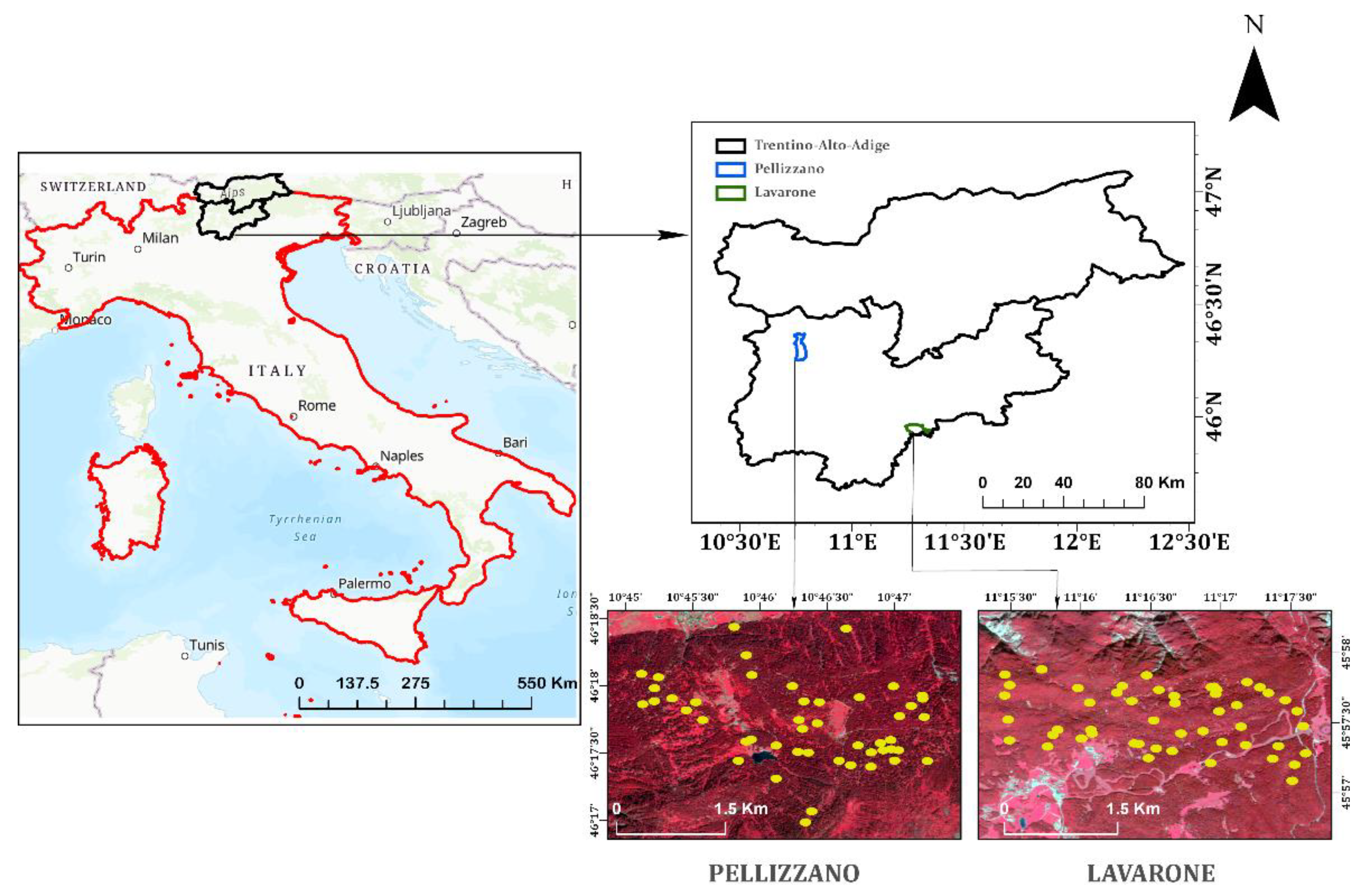
2.1. Study Area Description

The study area includes two sites, Lavarone and Pellizzano, both located in the Province of Trento, Italy, in the southern Alps. The forest in Lavarone is an uneven aged forest located at an altitude ranging from 1200 to 1600 m with species such as Norway spruce (Picea abies (L.) Karst.) and silver fir (Abies alba Mill.) accounting for 80% of the tree population and European beech (Fagus sylvatica L.), European larch (Larix decidua Mill.), and Scots pine (Pinus sylvestris L.) accounting for the remaining 20% of the population. The forest of Pellizzano is spread over an altitude from 900 to 2200 m and has a dominant presence of Norway spruce and subdominant presence of some coniferous species (e.g., Abies alba Mill., Larix decidua Mill., Pinus cembra L., Pinus sylvestris L., and Pinus nigra J., Arnold) and broadleaves species (Populus tremula L., Betula spp.). The forest is multilayered, more mixed, and structurally complex at lower altitudes and sparse at higher altitudes. The study was conducted in two areas to consider different species and the density of the forest. The geographical locations of both the study areas are shown using detailed maps in Figure 1.

2.2. Field Data

The field data for the Lavarone study area were collected on multiple days of summer of 2016 for 41 circular plots of 30 m diameter, and for the Pellizzano study area, were collected on multiple days of summer 2014 for 47 circular plots of 30 m diameter distributed over the entire study area. The plot coordinates were recorded using a survey grade Global Positioning System (GPS) unit. The field plots were distributed randomly across the forest area to be statistically significant. Inside each plot position, the diameter at breast height (DBH) and the height of each tree were measured, along with the species. The DBH threshold was kept at 3 cm (i.e., all trees above 3 cm were measured), and dead trees were included, but their presence was minimal. The AGB of each tree was computed using the allometric equations stated in [65] (also presented in Appendix A) and then aggregated for each plot to obtain the plot’s AGB. The AGB of the Lavarone field plots used for the study ranged from 69.42 to 412.34 Mg ha⁻¹, and the Pellizzano field plot AGB ranged from 0.9 to 545.3 Mg ha⁻¹. The mean tree height, mean tree DBH, and number of trees per plot for both the study areas are stated in

Table 1. Mean tree height, mean tree diameter at breast height (DBH), and number of trees per plot for both study areas.

		Lavarone	Pellizzano
Mean tree height per plot (m)	Minimum	7.43	5.94
	Maximum	27.29	37.9
	Mean	16.85	20.58
Mean tree DBH per plot (cm)	Minimum	10.71	8.78
	Maximum	37.83	57.17
	Mean	21.24	31.68
Number of trees	Minimum	17	2
	Maximum	192	147
	Mean	76.1	40.15

.

2.3. Remote Sensing Datasets

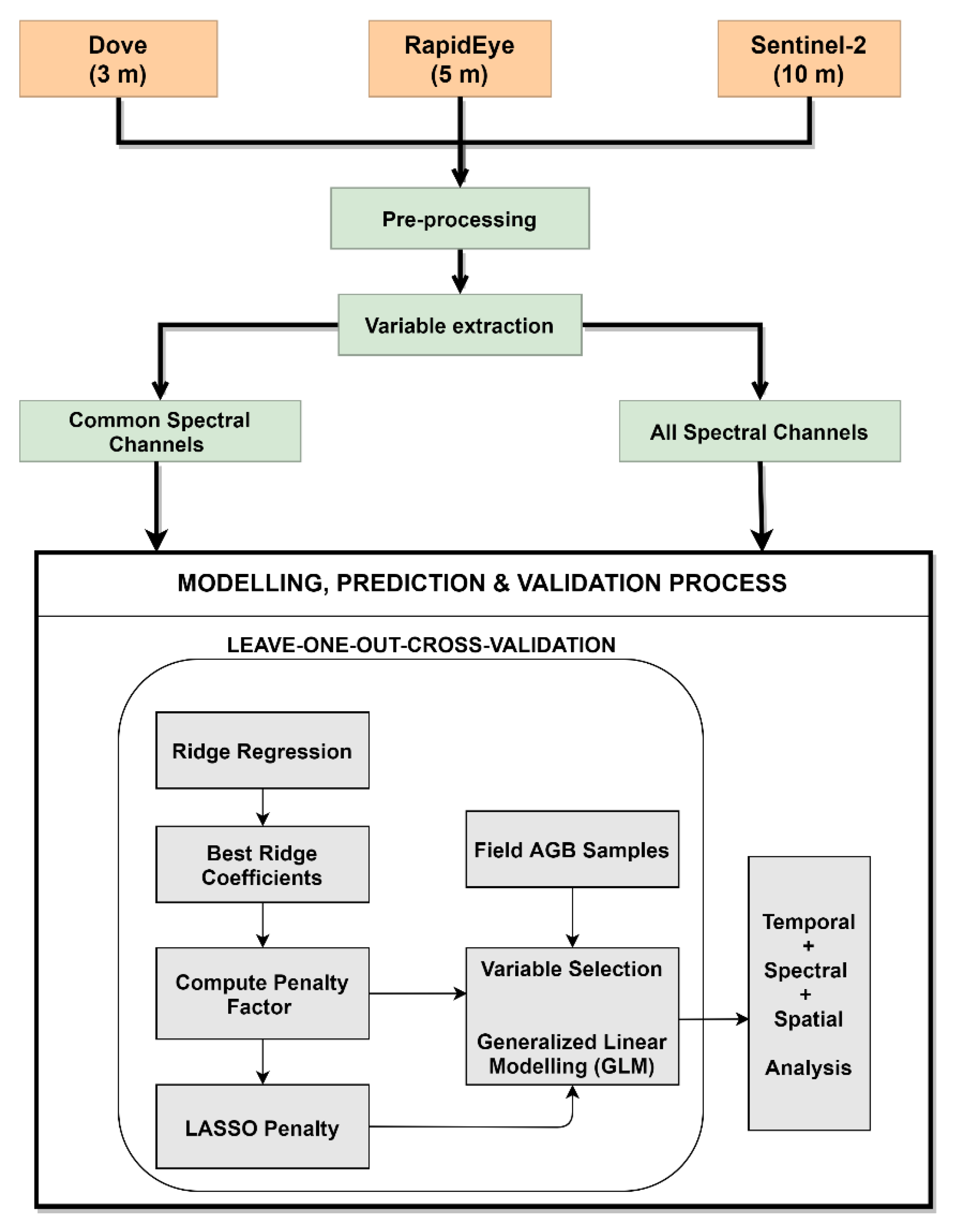
The Sentinel-2 data are acquired by twin satellites under ESA’s Copernicus program with a revisit capacity of 5 days. Sentinel-2 images are characterized by 13 spectral bands with four bands at 10 m, six bands at 20 m, and three bands at 60 m spatial resolution. In this study, we used 4 spectral bands at 10 m and 6 spectral bands at 20 m resampled to 10 m in the Blue, Green, Red, Red-edge, NIR, and Short wave infrared (SWIR) region.

The RapidEye data are acquired by a constellation of five satellites, operated by the Planet Labs Inc., with a multispectral push-broom imager capturing five spectral bands: Red, Green, Blue, NIR, and Red-Edge. The RapidEye satellites are identically calibrated so that the images acquired by the five satellites are indistinguishable from each other. Most of the acquired data have a view angle smaller than 10 degrees, and for all images, it is always less than 20 degrees. The ground sampling distance (nadir) is 6.5 m, and the orthorectified pixel size is of 5 m. The constellation of satellites acquires data with a daily revisit capacity (off-nadir) and 5.5 days at nadir.

The Dove data are acquired by a constellation of 120 Nano-satellites operated by Planet Labs Inc., with a daily revisit capacity. The satellites are deployed at the International space station (ISS) orbit at an inclination of 52 degrees and Sun synchronous (SS) orbit with an inclination of 98 degrees. The multispectral data are acquired using a Bayer-masked Charge-Coupled Device (CCD) camera with ground sampling distance (nadir) of 2.7–3.2 m in the ISS orbit and 3.7–4.9 m in the SS orbit. The orthorectified pixel size of the acquired images is 3 m with 4 spectral bands: Red, Green, Blue, and NIR.

The dates of multitemporal acquisition of multispectral data are stated in

Table 2. Acquisition dates (YYYY-MM-DD) of the multispectral data used in the study.

Seasons	Dates of Acquisition (Lavarone)			Dates of Acquisition (Pellizzano)
	Sentinel-2	RapidEye	Dove	Sentinel-2	RapidEye	Dove
Summer	2016-07-18	2016-07-29	2016-07-11	2016-07-18	2016-07-17	2016-08-22
Autumn	2016-10-16	2016-10-16	2016-10-20	2016-10-16	2016-10-21	2016-10-07
Winter	2017-01-07	2017-01-16	2017-01-23	2017-01-24	2017-01-16	2017-01-24
Spring	2017-04-07	2017-04-30	2017-04-23	2017-04-14	2017-04-22	2017-04-10

. There was a time gap between the field sampling and the used remotely sensed data to keep the temporal acquisitions of different satellite data consistent considering their availability. The field estimated annual increment in the diameter at breast height (DBH) was 2.8% [66]. Therefore, the increment of AGB sampled forest plots during the time gap can be considered as negligible and hence, admissible for the proposed experiments.

3. Methodology

The methodological flowchart of the study is shown in Figure 2. In the following sections, each step is described in detail.

3.1. Pre-Processing

Level-1C (Top-of-Atmosphere reflectances in cartographic geometry) data for Sentinel-2 data were gathered from the Copernicus open hub platform of European Space Agency (ESA) and converted to Level-2A (Bottom-of-atmosphere), which were atmospheric and terrain corrected using Sen2cor plugin. The bands at 20 m spatial resolution were resampled at 10 m using nearest neighbor sampling to adjust the pixel size to have a uniform band stack and simplified computation. Level-3A (orthorectified, geometrically corrected, and radiometrically calibrated) RapidEye and Dove images were gathered from the data access portal of Planet Labs (https://www.planet.com/explorer/) (accessed on 26 March 2021). The individual data bands for each dataset were mosaicked and stacked together to get a single data frame for both satellite images for all seasons.

3.2. Variable Extraction

Two sets of variables were considered for each multispectral dataset: the original band reflectances and the vegetation indices. The band reflectances of Sentinel-2 from B2 to B8 represent Blue, Green, Red, Vegetation red edge—1, 2, 3, and NIR, respectively; B8A represents narrow NIR, and B11 to B12 represent SWIR-1, 2 channels, respectively. The spectral reflectances of RapidEye from B1 to B5 represent Blue, Green, Red, Red edge, and NIR channels, respectively. The spectral reflectances of Dove from B1 to B4 represent Blue, Green, Red, and NIR channels, respectively. Numerous vegetation indices have been defined for specific applications in the literature [67,68,69]. To limit the number of predictor variables from the large number of existing vegetation indices, we selected 25 indices that were found to be robust in previous studies [70,71,72]. These 25 indices are stated in

Table 3. Vegetation indices and their equations used as variables for modeling.

Vegetation Indices	Equations
Canopy Chlorophyll Content Index	$\mathrm{CCCI}=\frac{\frac{\mathrm{NIR}-\mathrm{RedEdge}}{\mathrm{NIR}+\mathrm{RedEdge}}}{\frac{\mathrm{NIR}-\mathrm{R}}{\mathrm{NIR}+\mathrm{R}}}$
Chlorophyll Index Red Edge	$\mathrm{CIRE}=\frac{\mathrm{NIR}}{\mathrm{RedEdge}}-1$
Chlorophyll Vegetation Index	$\mathrm{CVI}=\mathrm{NIR} \frac{\mathrm{R}}{{\mathrm{G}}^2}$
Green Atmospherically Resistant Vegetation Index	$\mathrm{GARI}=\frac{\mathrm{NIR}-\left(\mathrm{G}-\left(\mathrm{B}-\mathrm{R}\right)\right)}{\mathrm{NIR}-\left(\mathrm{G}+\left(\mathrm{B}-\mathrm{R}\right)\right)}$
Green Leaf Index	$\mathrm{GLI}=\frac{2\mathrm{G}-\mathrm{R}-\mathrm{B}}{2\mathrm{G}+\mathrm{R}+\mathrm{B}}$
Log Ratio	$\mathrm{logR}=\log \frac{\mathrm{NIR}}{\mathrm{R}}$
Normalized Difference Vegetation Index	$\mathrm{NDVI}=\frac{\mathrm{NIR}-\mathrm{R}}{\mathrm{NIR}+\mathrm{R}}$
Normalized Burn Ratio	$\mathrm{NBR}=\frac{\mathrm{NIR}-\mathrm{SWIR}}{\mathrm{NIR}+\mathrm{SWIR}}$
Green Blue NDVI	$\mathrm{GBNDVI}=\frac{\mathrm{NIR}-\left(\mathrm{G}+\mathrm{B}\right)}{\mathrm{NIR}+\mathrm{G}+\mathrm{B}}$
Green Red NDVI	$\mathrm{GRNDVI}=\frac{\mathrm{NIR}-\left(\mathrm{G}+\mathrm{R}\right)}{\mathrm{NIR}+\mathrm{G}+\mathrm{R}}$
Red Blue NDVI	$\mathrm{RBNDVI}=\frac{\mathrm{NIR}-\left(\mathrm{R}+\mathrm{B}\right)}{\mathrm{NIR}+\mathrm{R}+\mathrm{B}}$
Green NDVI	$\mathrm{GNDVI}=\frac{\mathrm{NIR}-\mathrm{G}}{\mathrm{NIR}+\mathrm{G}}$
Red Edge NDVI	$\mathrm{NDVIre}=\frac{\mathrm{NIR}-\mathrm{RedEdge}}{\mathrm{NIR}+\mathrm{RedEdge}}$
Pan NDVI	$\mathrm{PNDVI}=\frac{\mathrm{NIR}-\left(\mathrm{R}+\mathrm{G}+\mathrm{B}\right)}{\mathrm{NIR}+\mathrm{R}+\mathrm{G}+\mathrm{B}}$
Visible Index Green	$\mathrm{VIgreen}=\frac{\mathrm{G}-\mathrm{R}}{\mathrm{G}+\mathrm{R}}$
Norm of X (X = R, G, NIR)	$\mathrm{Norm} \mathrm{X}=\frac{\mathrm{X}}{\sum \mathrm{X}}$
Blue-Wide Dynamic Range Vegetation Index	$\mathrm{BWDRVI}=\frac{0.1 * \mathrm{NIR}-\mathrm{B}}{0.1 * \mathrm{NIR}+\mathrm{B}}$
Chlrophyll Index Green	$\mathrm{CIgreen}=\frac{\mathrm{NIR}}{\mathrm{G}}-1$
Green Difference Vegetation Index	$\mathrm{GDVI}=\mathrm{NIR}-\mathrm{G}$
Blue Normalized Vegetation Index	$\mathrm{BNDVI}=\frac{\mathrm{NIR}-\mathrm{B}}{\mathrm{NIR}+\mathrm{B}}$
Redness Index	$\mathrm{RI}=\frac{\mathrm{R}-\mathrm{G}}{\mathrm{R}+\mathrm{G}}$
Difference Vegetation Index or Vegetation Index Number	$\mathrm{DVI}=\frac{\mathrm{NIR}}{\mathrm{R}}$
Specific Leaf Area Vegetation Index	$\mathrm{SLAVI}=\frac{\mathrm{NIR}}{\mathrm{R}+\mathrm{SWIR}}$

R = Red; G = Green; B = Blue; NIR = Near Infra-red; RedEdge = Red Edge; SWIR = Short-wave infrared; NDVI = Normalized Difference Vegetation Index.

with their respective equations.

All these variables were extracted for each circular ground plot of 30 m diameter, and to match the ground sample plots with remote sensing data at different spatial resolutions, we aggregated the pixels (at 3, 5, and 10 m according to the satellite considered) inside each plot by making the average of the spectral values in each band/index. In particular, we used the “gBuffer” function of the “rgeos” library in R. A round cap style with 15 m radial size was used for the inclusion of pixels within the area of the field plots and only the pixels that overlap with the size of the plot on the ground were considered.

3.3. Variable Selection, Modeling, and Validation

Variable selection is a way to reduce the number of predictor variables to reduce the model complexity to mitigate the overfitting problem. In this study, we considered a total of 25 vegetation indices and all available band reflectances as predictor variables for modeling AGB. A robust adaptive lasso (least absolute shrinkage and selection operator) technique that uses L1 penalization method was implemented to perform automated variable selection. The adaptive lasso estimator ${\hat{\mathbf{\beta }}}^{LS}$ [73] is stated in Equation (1):

$${\hat{\beta }}^{LS}=\underset{\beta \in {\mathbb{R}}^p}{\arg min}{\Sigma }_{i=1}^n{(Y_i-{\mathrm{X}}_i^T\beta )}^2+\lambda {\Sigma }_{j=1}^p{\omega }_j\left|{\beta }_j\right|$$

(1)

Here, $\lambda >0$ is the tuning parameter (penalty parameter) and ${\omega }_j$ is the given adaptive weighted vector that needs to be tuned to achieve accurate estimates with a small error. The term $\left(Y_i-{\mathrm{X}}_i^T\beta \right)$ represents a random sample having identical independent distribution associated with regression coefficients $\prime {\beta }^{\prime }$.

Initially, we used ridge regression for computing the best ridge coefficients at a minimum value of $\lambda$ parameter. We then calculated the penalty factor using the best ridge coefficients. Next, we performed adaptive lasso with the calculated penalty factor using lasso penalty. The penalty factor was used to tune the $\lambda$ to allow a differential shrinkage. The penalty factor can be ‘0’ for some predictor variables with the lasso penalty that implies no shrinkage and inclusion of that particular predictor variable in the model. Thus, adaptive lasso uses lasso penalty to push the coefficient of predictor variables to absolute ’0’, which improves the model by selecting the most consistent variables and automates the process of variable selection.

A generalized linear modeling [74] approach via penalized maximum likelihood was used for associating selected variables with the target AGB values. The modeling algorithm uses cyclical coordinate descent to optimize the objective function over each parameter successively for convergence. To achieve the objective of the study, we computed 6 metrics for assessing the precision, the agreement, and the overfitting of models. The cross validation metrics, their equations, and the related assessment aspect is stated in

Table 4. Assessment metrics computed using Leave-One-Out Cross-Validation (LOOCV).

Accuracy statistics	Equations	Assessment Role
Mean absolute difference	$MAD={\displaystyle {\displaystyle \sum }_{i=1}^n}\left|pr{e}_i^{CV}-ob{s}_i\right|/n$	Prediction precision
Root mean squared differences	$RMSD=\sqrt{\frac{S{S}^{CV}}{n}}$	Prediction precision
Coefficient of determination (residuals)	$R_{fit}^2=1-S{S}_{fit }/ S{S}_{tot}$	Agreement
Coefficient of determination (cross-validation)	$R_{CV}^2=1-S{S}^{CV}/S{S}_{tot}$	Agreement
R2 Ratio	$R2R=R_{fit}^2/R_{CV}^2$	Overfitting
Sum of squares ratio	$SSR=\frac{\sqrt{S{S}^{CV}}}{\sqrt{S{S}^{fit}}}$	Overfitting

n: total number of samples; pre_i^cv: prediction value of sample i obtained by cross validation; obs_i: observed value of sample i; SS^CV: sum of squared differences between observed and predicted values by cross validation; SS^fit: sum of squares of model residuals; SS^tot: sum of squared differences of each observation from the overall mean.

. The entire process starting from computing ridge coefficients to computing assessment metrics, was performed by using leave-one-out cross validation. A mean squared error measure was used to calculate the loss of cross validation. We used R-packages—‘tidyverse’, ‘magrittr’, ‘glmnet’, ‘pROC’, ‘mgcv’, and ‘ggplot2’ to conduct the entire process of variable selection, modeling, validation, and graphing.

3.4. Design of Experiments

The designed experiments were aimed at analyzing the effect of temporal, spectral, and spatial capacities of multispectral satellite data for the prediction of AGB.

The temporal analysis was carried out using the generalized linear modeling on common spectral channels, i.e., by only using RGB and NIR bands of each satellite data. This was done to remove the effects of extra channels present in Sentinel-2 and RapidEye data as compared to Dove data. The modeling was done for each single-time image, thus obtaining one model for each season. In addition, we also performed modeling on multitemporal data (i.e., considering all images combined) to observe the effect of temporal information on the AGB prediction. The effects of temporal information were assessed based on the metrics defined in Table 2.

The spectral analysis was carried out using the generalized linear modeling on data from all available spectral channels of each satellite sensor. The effect of spectral channels was assessed using variables selected by the adaptive lasso algorithm and the agreement of selected variables with AGB using the coefficient of determination. Variables were divided into three groups according to the part of the spectrum they belong to—the common (RGB and NIR) channels, the Red-edge channels, and the SWIR channels.

The spatial analysis was carried out by analyzing scatter plots of the most frequently selected key variables computed at 3, 5, and 10 m spatial resolution with AGB. A Pearson correlation coefficient (R) was computed to observe the change in the agreement between the selected key variables at different spatial scales with the AGB.

4. Results

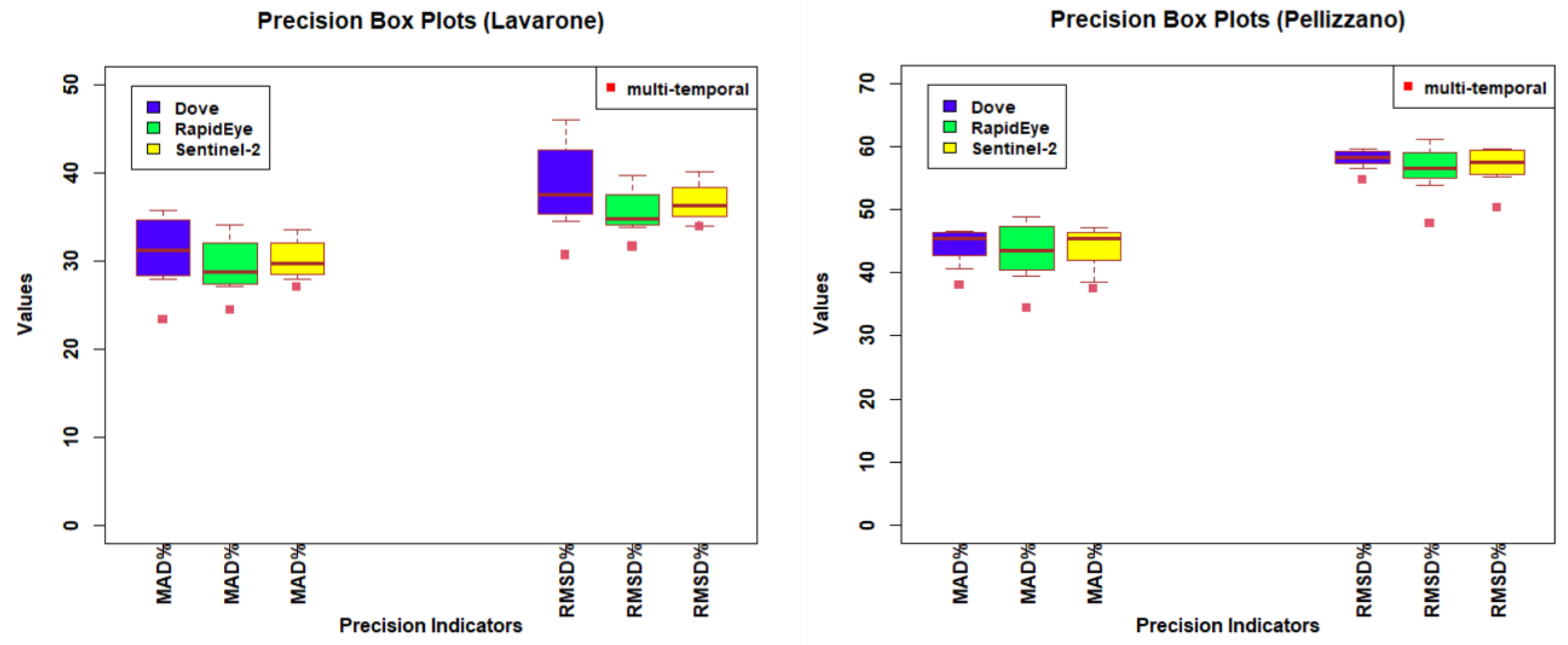
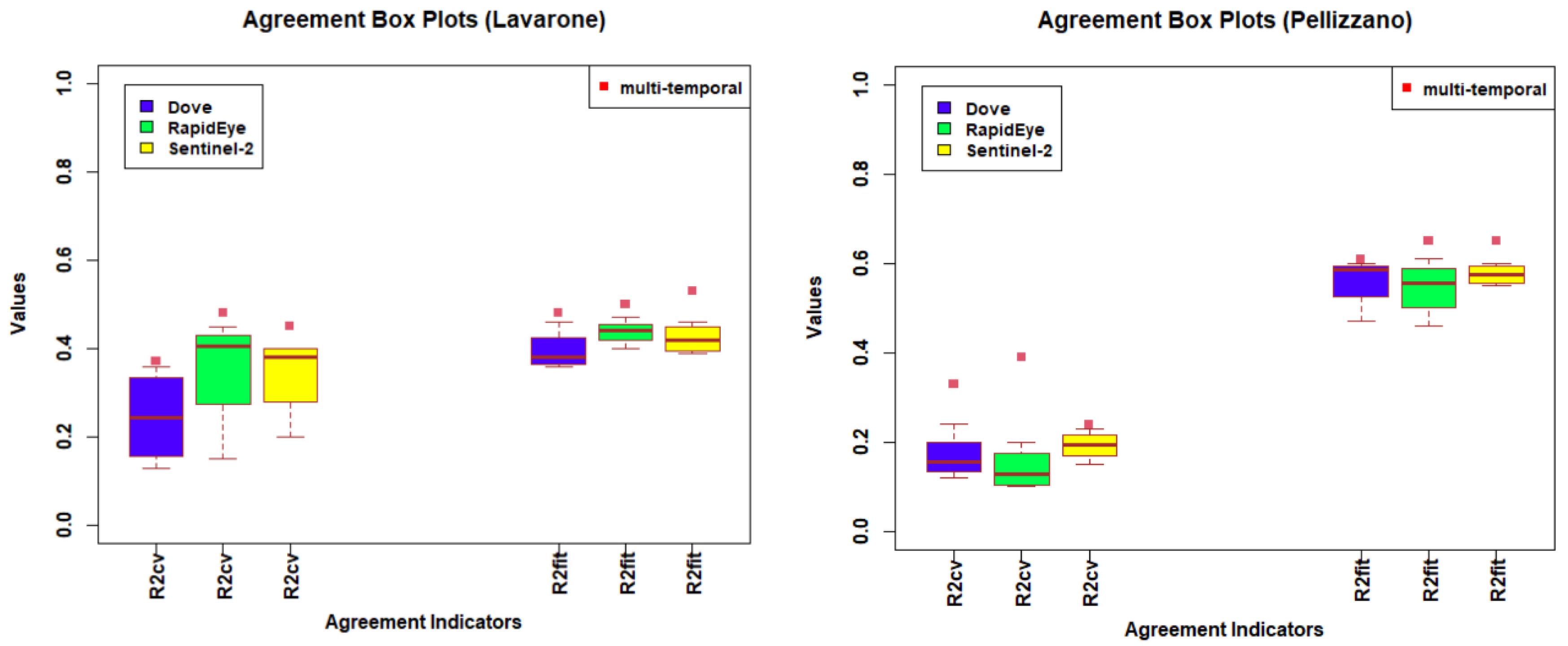
4.1. Temporal Analysis

The effect of temporal information was analyzed using box plots depicting the variation of precision, agreement, and overfitting computed with generalized linear modeling on data from common spectral channels of the three satellites (RGB and NIR) using six metrics stated in Table 2. The precision box plots (Mean Absolute Difference % (MAD%), Root Mean Squared Difference % (RMSD%)) shown in Figure 3 depict that all single-time models had lower prediction precision as compared to the multitemporal models. The analysis indicates that all satellite data had improved prediction precision due to the inclusion of multitemporal information in the model for both the study areas. The addition of multitemporal information showed more significant improvement for Dove (in Lavarone) and RapidEye (in Pellizzano) data that are characterized by higher spatial resolution. All single-time models showed high variance in the prediction precision. This indicates a significant influence of specific seasons of data acquisition for AGB modeling.

Figure 4 shows the agreement box plots (R2fit, R2cv), pointing out that all multitemporal models performed better than single-time models for both the study areas. Although the temporal information improved performance of different datasets at different magnitudes, a significant improvement was observed for Dove and RapidEye data in the Pellizzano area, where the R2cv doubled the average R2cv of single-time models. The variance in the agreement of all single-time models provides a clear advantage for the use of multitemporal multispectral data for AGB prediction.

Regarding the overfitting box plots shown in Figure 5, the desirable values of R-squared Ratio (R2R) and Sum of Squares Ratio (SSR) should be less than 1.1, wherein the real (cross-validated) precision exceeded 10% of the model residual variance. For most cases, the multitemporal models achieved less overfitting as compared to single-time models. In addition, the overfitting box plots depict considerable uncertainty for single-time models and certain dependence on the spatial location that indirectly influence the distribution of field plot AGB values. This effect can be observed clearly for the two different study areas where Lavarone had a high variance in overfitting indicators for all data, whereas comparatively low variance was observed for Pellizzano. However, all multitemporal models resulted in an acceptable level of overfitting, proving the effectiveness of temporal information.

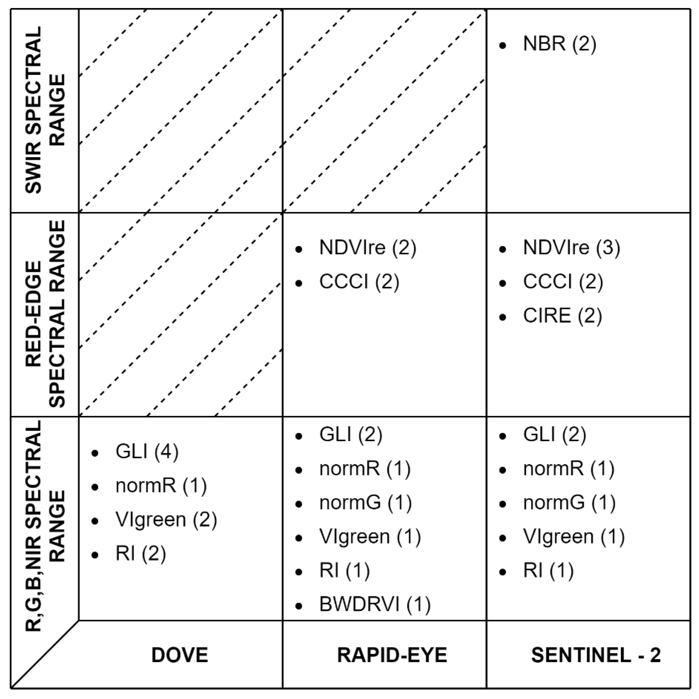
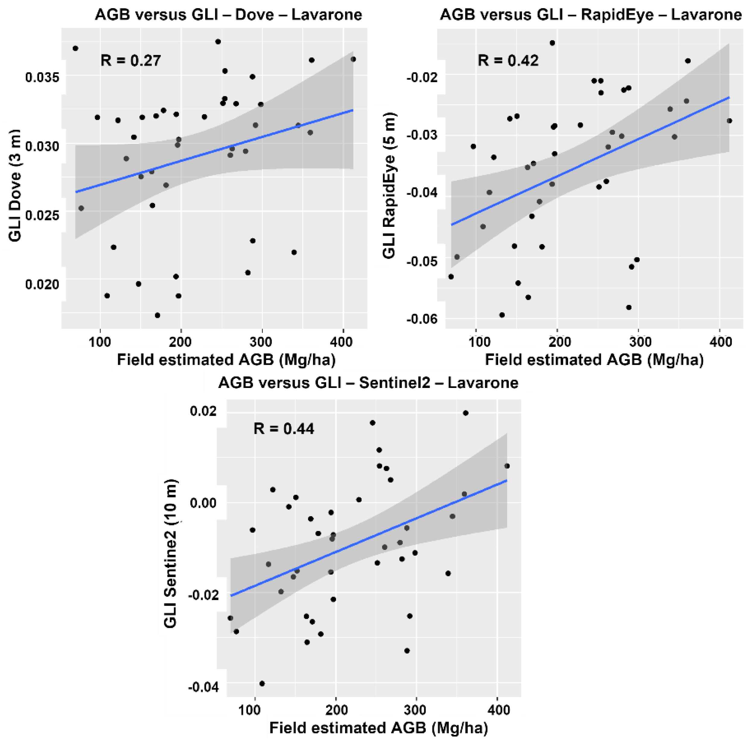
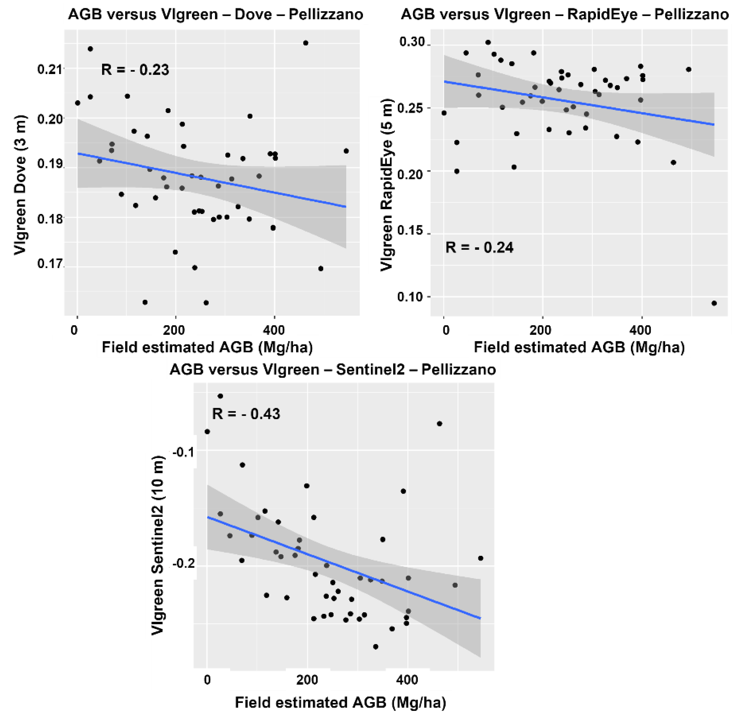
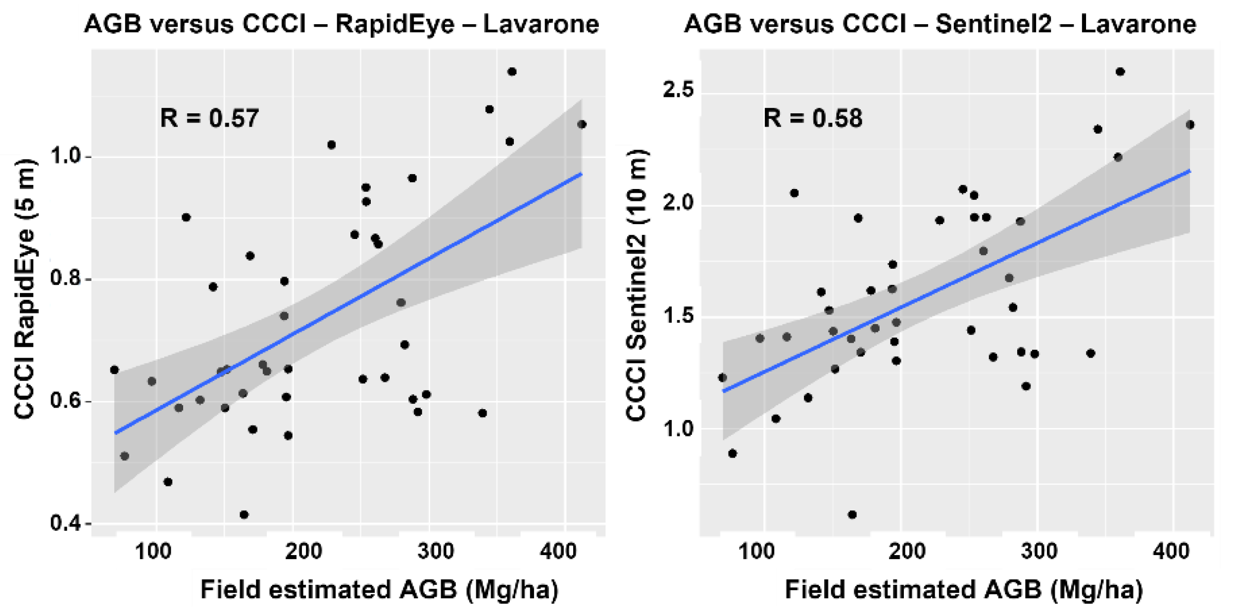
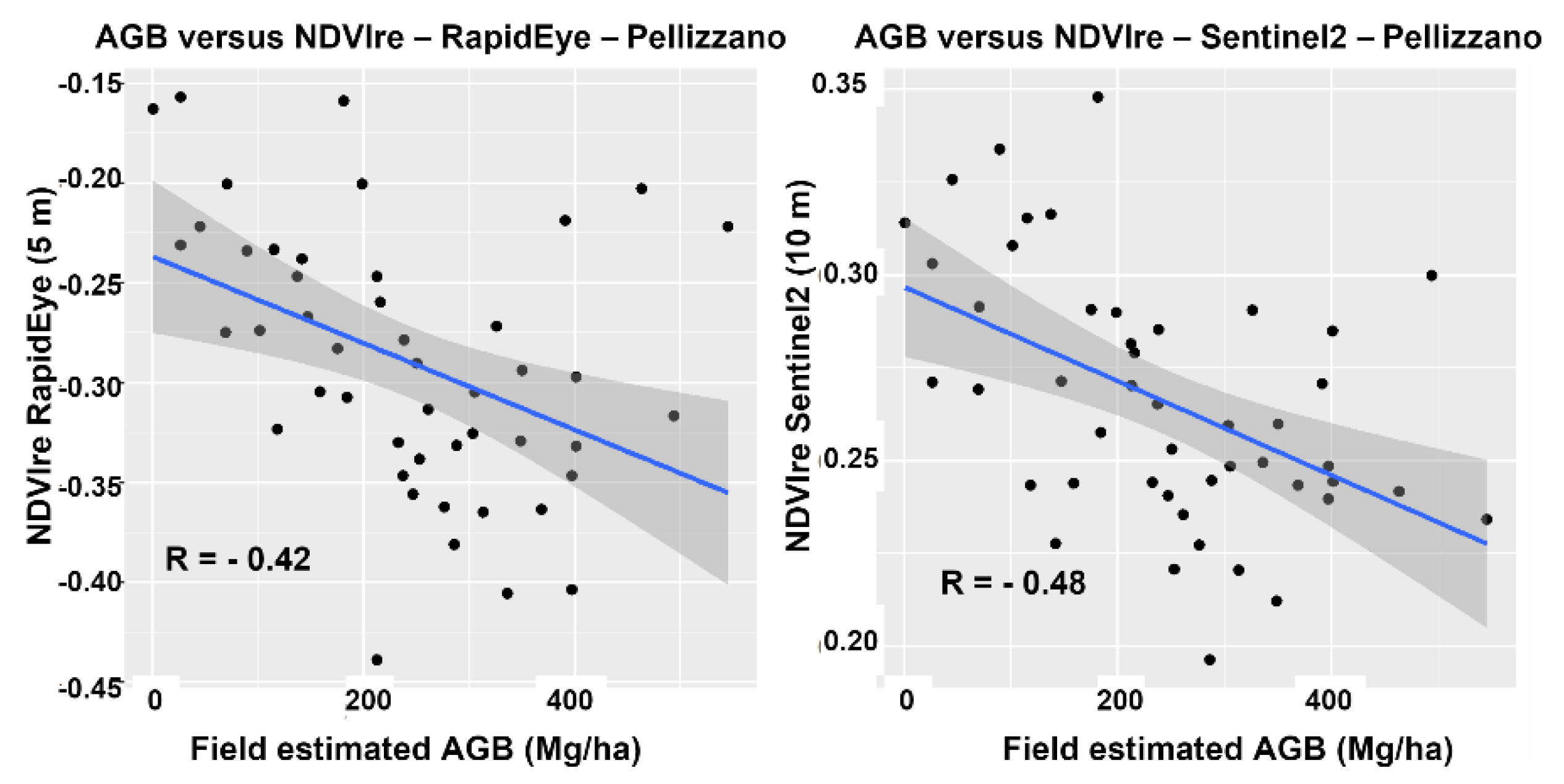
4.2. Spectral Analysis

The spectral analysis was carried out for multitemporal models using variable selection applied to all available spectral channels with the adaptive LASSO algorithm. Figure 6 represents the variables selected for all the datasets for both the study areas, and values in the round bracket show their frequency of occurrence. The values of the multi-time selected variables maybe different depending upon the season, and their selection was purely based on the adaptive LASSO algorithm applied to the entire set of variables under consideration. For clear visualization of spectrum specific selection, the selected variables have been divided into three spectral ranges associated with RGB and NIR channels, Red-edge channels, and the SWIR channels. Figure 7 and Figure 8 show the regression plots (Field estimated AGB vs. Predicted AGB) with a cross validated coefficient of determination for Lavarone and Pellizzano area, respectively.

For the Dove data, four variables were primarily selected by the adaptive LASSO algorithm for multitemporal models of both study areas. The Green Leaf Index (GLI) variable formulated using the RGB channels was the most frequently (four times) selected among all variables. The other two variables more frequently selected were VIgreen (two times) and RI (two times). It is interesting to note that these three frequently selected variables for the Dove data were formulated without the NIR channel. The agreement achieved on the scale of coefficient of determination were 0.37 and 0.33 for Lavarone and Pellizzano, respectively. For the RapidEye data, eight variables were selected in total for both multitemporal models. There were three variables selected twice, namely GLI, Red Edge NDVI (NDVIre), and Canopy Chlorophyll Content Index (CCCI), two out of which (NDVIre and CCCI) were formulated using the red-edge channels. The red-edge channels contributed to the significant improvement in the agreement of RapidEye models over Dove models. The agreement achieved for RapidEye based multitemporal models was 0.51 and 0.44 for Lavarone and Pellizzano, respectively. For the Sentinel-2 data, the NDVIre formulated using the red-edge channels was the most frequently selected variable. The other most frequently selected variables GLI, CCCI, Chlorophyll Index Red Edge (CIRE), and Normalized Burn Ratio (NBR) were all selected twice for the two multitemporal models. CCCI and CIRE were formulated using the red-edge channels, whereas NBR was formulated using the SWIR channel. The red-edge and the SWIR channels contributed to more than 50% of the total selected variables. This involved a more significant improvement in the agreement of models as compared to both RapidEye and Dove. The coefficient of determination was computed for multitemporal models as 0.53 and 0.51 for Lavarone and Pellizzano, respectively.

To sum up, GLI was the most consistently selected variable for all three satellite data. Sentinel-2 data achieved the highest agreement in modeling as compared to RapidEye and Dove. Moreover, Red-edge and SWIR channels significantly improved the modeling accuracy for the prediction of AGB.

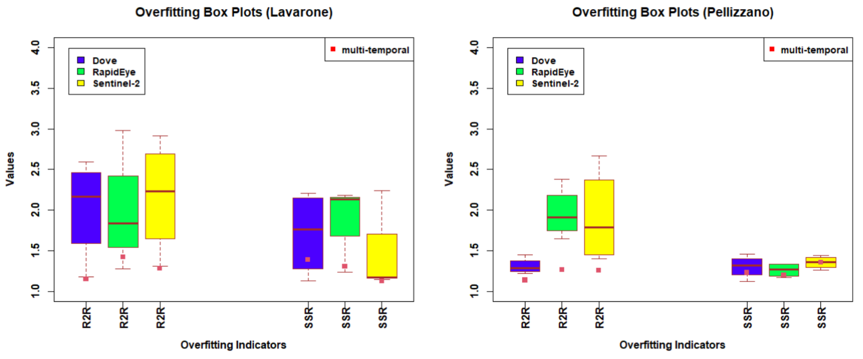
4.3. Spatial Analysis

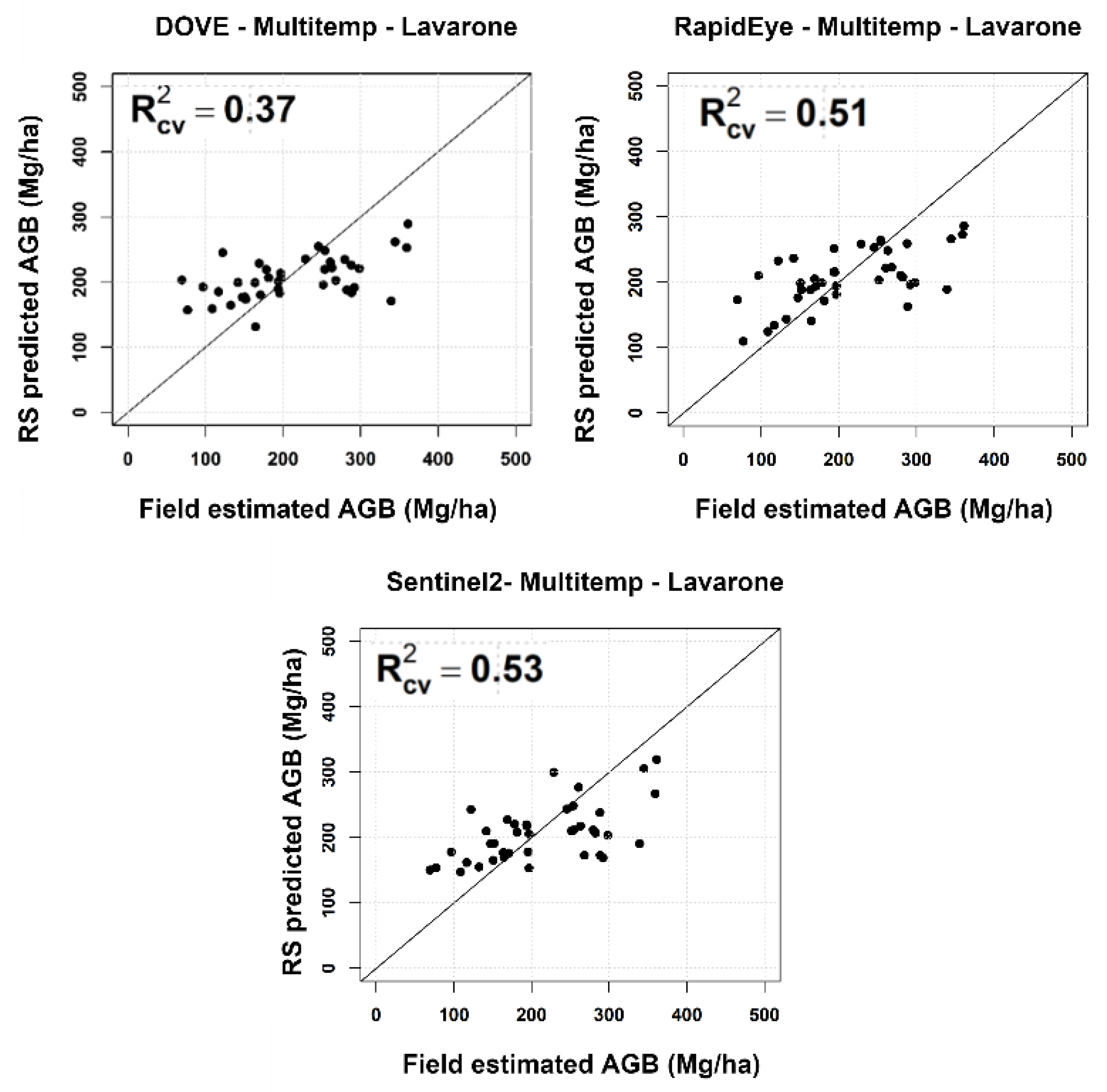
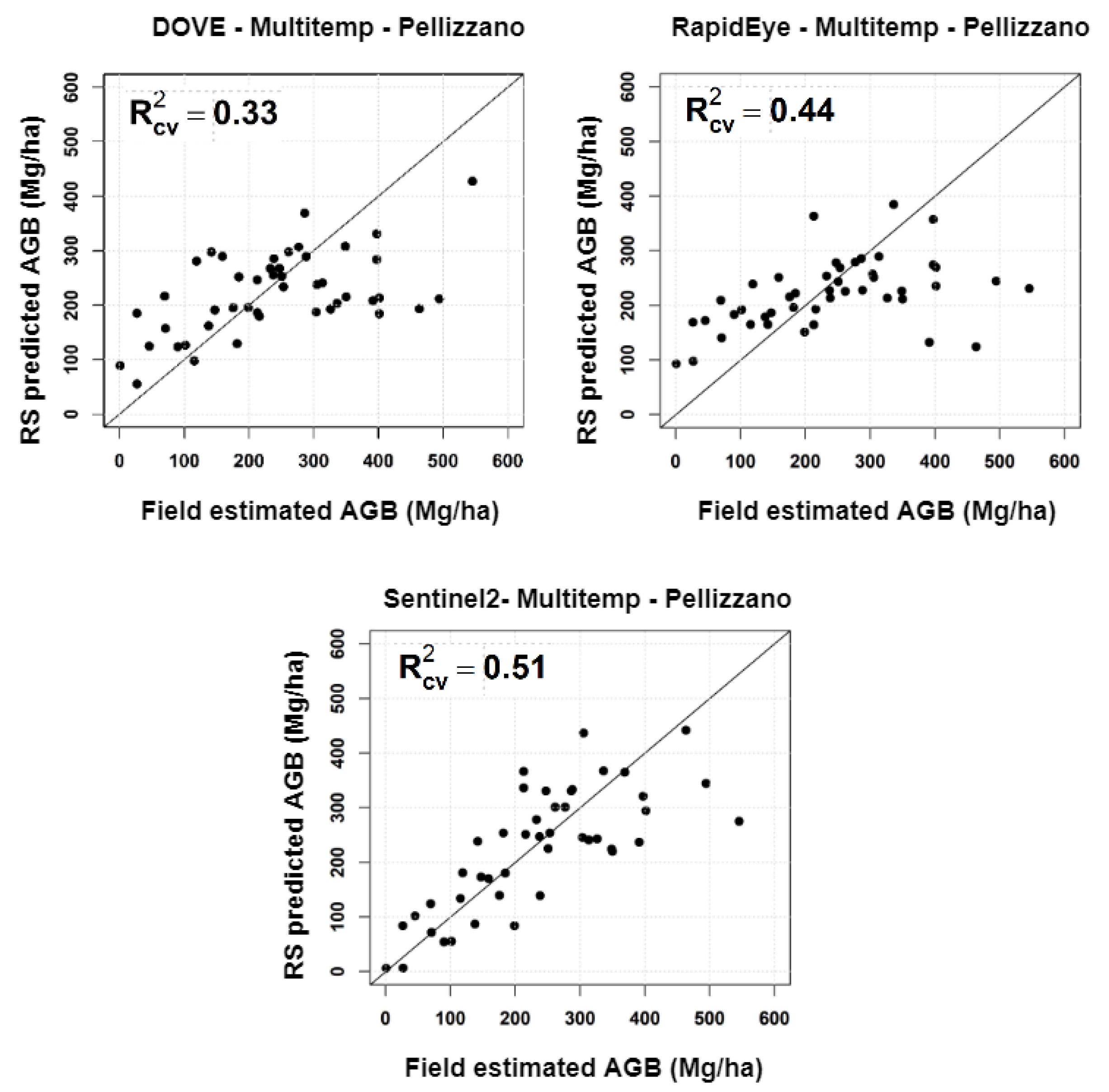
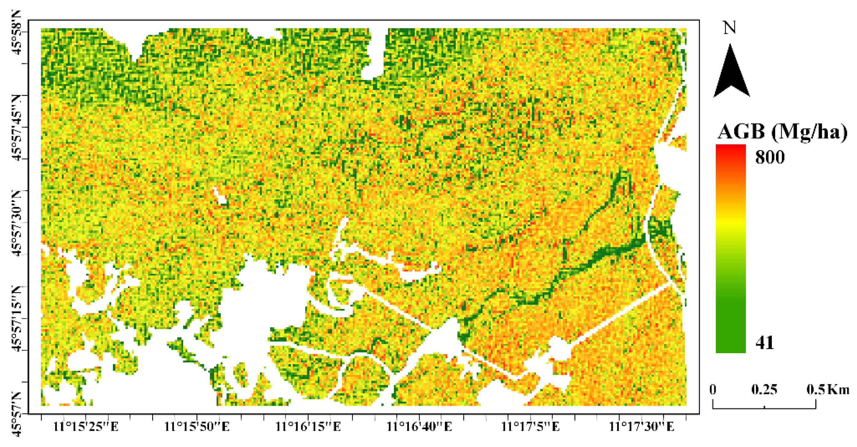
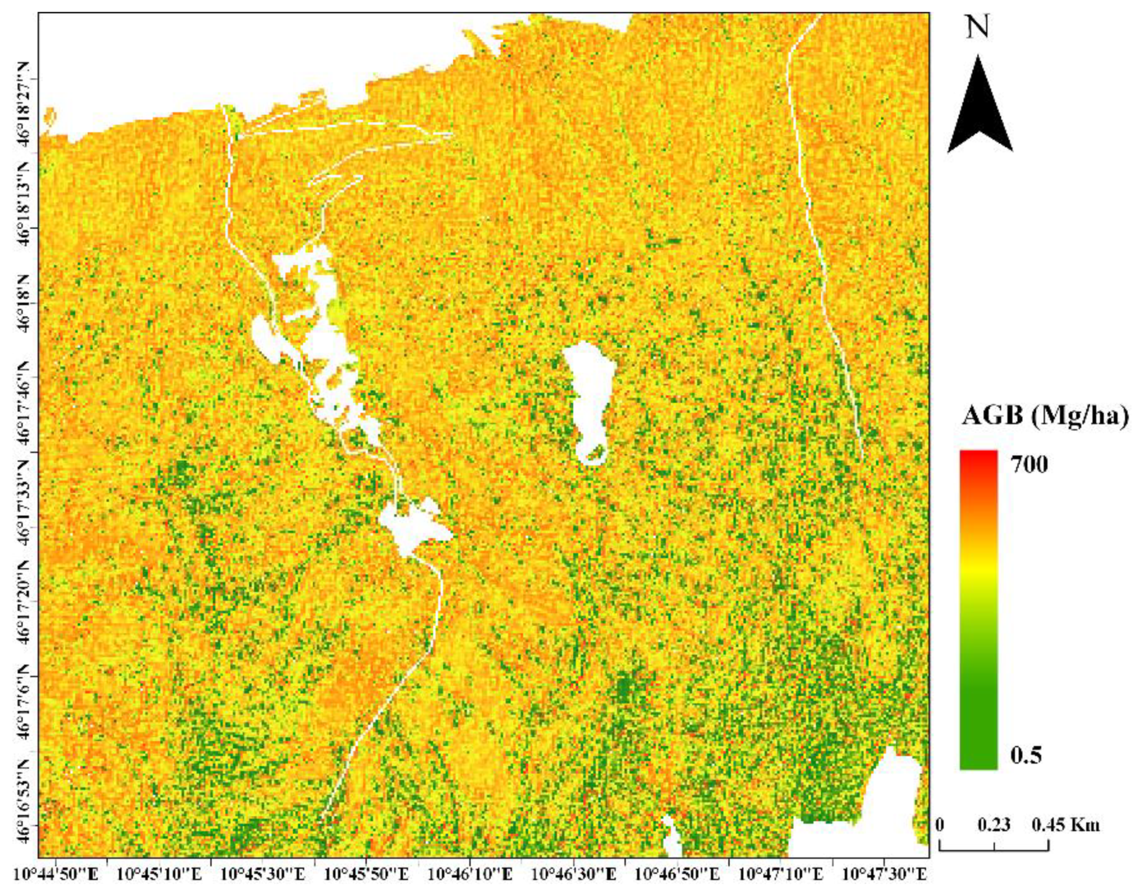
The analysis of the effects of spatial resolution on AGB estimation was carried out by observing the change in the correlation of key variables determined by Pearson’s correlation coefficient (R) at different spatial scales. Figure 9 shows the scatter plots of GLI (autumn) vs. AGB at 3, 5, and 10 m for the Lavarone area, and Figure 10 shows the scatter plots of Visible Index Green (VIgreen) (summer) vs. AGB at 3, 5, and 10 m for the Pellizzano area.

The analysis of scatter plots in Figure 9 and Figure 10 collectively suggest a higher correlation of the considered key variables at 10 m, i.e., at a lower spatial scale. A correlation of 0.44 and −0.43 was achieved for GLI (autumn) and VIgreen (summer) variables, respectively, at 10 m which was higher in comparison to those achieved at 5 and 3 m.

Figure 11 and Figure 12 present the scatter plots for key variables in the red-edge spectral range with the field estimated AGB. Figure 11 shows the scatterplot of CCCI (spring) variable, and Figure 12 shows the scatter plot of NDVIre (spring) at 5 and 10 m for Lavarone and Pellizzano, respectively. A similar trend was observed for key variables in the red-edge spectrum, with the highest correlation observed at 10 m spatial resolution. The highest correlation observed for CCCI (spring) was 0.58 and for NDVIre (spring) was −0.48 at 10 m. Though there was no significant difference for CCCI (spring) at 5 m, a significant difference in correlation was observed for NDVIre (spring).

4.4. AGB Maps

To visualize the spatial distribution of the predicted AGB over the selected study areas, we used the multitemporal data based models developed using Sentinel-2 images with the best modeling accuracy for both study areas. The AGB maps for Lavarone and Pellizzano are shown in Figure 13 and Figure 14, respectively. In the maps, the non-forest areas were masked.

As one can observe from the AGB maps, there were areas having higher AGB, corresponding with more mature and dense forest, and areas with lower AGB corresponding with sparser and young forest. In particular, in the Lavarone forest, the Northern part of the map was at a higher altitude, and the forest there was sparser and less productive. Similarly, in the Pellizzano forest, the Southern part of the map was the one at the highest altitude, characterized by a sparse forest of Larch and Stone pine.

5. Discussion

In this study, we modeled AGB using spectral features extracted from multispectral satellite data at various spatial scales from medium to high spatial resolution. We analyzed the prediction results with respect to temporal, spectral, and spatial properties of different multispectral data and assessed their potential in the prediction of AGB. The results obtained in this study could be used as guidelines for the use of multispectral data in the prediction of AGB and support some of the results obtained in previous studies.

For example, in [75], the single-time spectral bands and spectral indices from the Sentinel-2 data were independently used to predict forest stock volume. A high range of prediction error was observed for all values greater than 300 m³ ha⁻¹ for most of the single-time models in the temporal analysis for the prediction of AGB. Our study shows the limitation of high variance in precision, agreement, and overfitting with inferior modeling results of single-time models and provides a solution in the form of multitemporal models. Multitemporal data provides additional information to the model on seasonal variations of the same spectral features. Multitemporal models for all datasets (Dove, RapidEye, and Sentinel-2) achieved better modeling accuracy than their respective single-time models. Therefore, adding the temporal information complemented the spectral features at all spatial scales for both the considered study areas characterized by different forest compositions. Despite the heterogeneous and complex forest ecosystem, the multitemporal models performed better as compared to single-time models. Moreover, the annual growth of the stem diameter, and hence, the AGB, is dependent on factors such as rainfall, temperature, humidity, day length, species, etc. [76], which directly affect the seasonal patterns of vegetation. Therefore, it can be stated that the seasonal variation in spectral reflectance of the forest plots captured using spectral features of multitemporal multispectral data is expected to have a relationship with the structural measures of the forest, and hence, the AGB. Based on similar assumptions, the studies [15,52,77] were previously performed on Landsat time-series data for the prediction of AGB. Our study adopted certain improvements in methodology and analytical approach to quantify the key aspects (i.e., precision, agreement, and overfitting observed in time) for improving the prediction of AGB. In addition, the temporal results were analyzed by developing experiments performed at various spatial scales (3, 5, and 10 m) of multispectral data.

The process of variable selection is crucial for modeling AGB with spectral features of multispectral data. A few studies [34,75,78,79,80] bypass the process of variable selection and produce models with large overfitting and high margin of errors. For example, in [34], to predict stand biomass using Landsat data, the models were developed separately for spectral bands and spectral indices without the use of any variable selection method. In [78], multiple variables were added to a basic model one at a time to determine an optimum combination model to predict forest stand volume. However, the most reliable way to add or remove a variable is to use a robust variable selection method. In this study, we systematically added variables to the models using an adaptive lasso variable selection method. Only specific robust variables driving significant change in the model were added. In [75], the forest stock volume was estimated from multispectral data with two different spatial resolutions. The two different models at two different spatial resolutions were developed based on single spectral variables having the highest correlation. Differently, in this study, we developed models based on the combination of different spectral variables at three different spatial resolutions using a robust variable selection method. Performing the spectral analysis experiment for two different study areas, the important role of some specific spectral bands in modeling AGB was iteratively determined.

A few other studies (e.g., [75,78,79,81]) were conducted on Sentinel-2 data using different modeling approaches for the prediction of forest biophysical parameters. In [81], Sentinel-2 data were used at 20, 40, and 60 m for the prediction of canopy cover using the same spectral indices. These indices achieved similar results at all spatial scales with identical scatterplots and equivalent RMSE values. In our study, we analyzed the correlation of a few selected key variables from different spectral ranges at different spatial resolutions. The observed significant variation in a correlation of the same key variables at different spatial resolutions pointed out an instrumental role of spatial resolution in the prediction of AGB. The key variables in all cases were more correlated at a lower spatial resolution, and thus, the higher spatial resolution of the data is less relevant when the prediction method is based on spectral features from multispectral data. Our study provides a solution to make AGB modeling at a higher spatial resolution more viable by including relevant spectral information. This can be observed from the modeling results presented in the spectral spatial analysis section of the study.

This study can assist geo-spatial startups, such as Planet Labs, and other space agencies in planning future missions with respect to onboard sensor equipment and upgrade for forest applications. The primary focus of this study was to explore the role of different capacities of multispectral data in modeling AGB, and therefore, the approach was limited to serve the objectives. In addition, this study can prove relevant and useful for the development of more efficient tools and techniques based on automatic feature extraction and selection with hierarchical modeling methods using multispectral data. There is a possibility of developing alternate tree-crown segmentation and texture variance based methods using high resolution multispectral images, which may prove effective even with limited spectral channels. Moreover, with respect to alternate spaceborne data for the prediction of AGB, long wavelength and cross-polarization in SAR may be comparable in terms of uncertainty, availability, and time of processing with state-of-the-art multispectral data. However, multispectral satellites provide better regional and global data consistency for complex canopies and forest cover on mountainous terrain. As shown in [19], SAR data used for four different study areas with three different polarizations produce uncertainty and variance in modeling accuracy for AGB prediction. In our study, a similar variance in modeling accuracy was observed at different temporal instances, and a small uncertainty was observed depending upon variables selected for multitemporal multispectral data. It is worth noting that different modeling approaches could have led to slightly different results. However, this would be the case for every chosen approach or the other different extracted features. Furthermore, the limited field plot samples could restrict model performance to some extent, as observed in this study. As the study was purely based on spectral data, a forest-type specific trained model would be required to make predictions at the global level. Despite these limitations, this study presented a systematic approach to variable extraction and automatic variable selection based on a robust algorithm and a consistent set of experiments to achieve the desired objectives. The results point out the potential of spectral data for AGB prediction. In the future, using this study as a basis, more sophisticated disentangled feature generation and integrated modeling approaches using deep learning can be developed.

6. Conclusions

In this study, different multitemporal multispectral remote sensing data were used to characterize the effect of temporal and spectral information as well as spatial resolution for predicting forest AGB. The results clearly showed that each characteristic of multispectral data affects the prediction of AGB. Multispectral data characterized by the spectral information from red-edge and SWIR channels in addition to the visible spectrum diminish the effect of data saturation and formulate effective predictors of AGB. The correlation of key variables at different spatial scales iteratively suggests better estimates of AGB at low spatial resolution ruling out a greater role of high spatial resolution in spectral variable based modeling. In addition, single-time based multispectral data are insufficient for accurately modeling AGB, and it requires multitemporal data for better modeling accuracy. The multitemporal models present a significant improvement over all single-time models confirming multispectral data as a fine and potent resource for AGB prediction.

References

1. Brown, S. Estimating Biomass and Biomass Change of Tropical Forests: A Primer; Food and Agriculture Organization: Rome, Italy, 1997; Volume 134, pp. 13–33. [Google Scholar]
2. Food and Agriculture Organization. National Forest Monitoring and Assessment: Manual for Integrated Field Data Collection; NFMA Working Paper; Food and Agriculture Organization: Rome, Italy, 2008; p. 206. [Google Scholar]
3. Chen, Q.; McRoberts, R. Statewide mapping and estimation of vegetation aboveground biomass using airborne lidar. In Proceedings of the 2016 IEEE International Geoscience and Remote Sensing Symposium (IGARSS), Beijing, China, 10–15 July 2016; pp. 4442–4444. [Google Scholar]
4. Ojoatre, S.; Zhang, C.; Hussin, Y.A.; Kloosterman, H.E.; Ismail, M.H. Assessing the Uncertainty of Tree Height and Aboveground Biomass from Terrestrial Laser Scanner and Hypsometer Using Airborne LiDAR Data in Tropical Rainforests. IEEE J. Sel. Top. Appl. Earth Obs. Remote Sens. 2019, 12, 4149–4159. [Google Scholar] [CrossRef] [Green Version]
5. Silva, C.A.; Saatchi, S.; Garcia, M.; Labriere, N.; Klauberg, C.; Ferraz, A.; Meyer, V.; Jeffery, K.J.; Abernethy, K.; White, L.; et al. Comparison of Small-and Large-Footprint Lidar Characterization of Tropical Forest Aboveground Structure and Biomass: A Case Study from Central Gabon. IEEE J. Sel. Top. Appl. Earth Obs. Remote Sens. 2018, 11, 3512–3526. [Google Scholar] [CrossRef] [Green Version]
6. Yang, L.; Liang, S.; Zhang, Y. A new method for generating a global forest aboveground biomass map from multiple high-level satellite products and ancillary information. IEEE J. Sel. Top. Appl. Earth Obs. Remote Sens. 2020, 13, 2587–2597. [Google Scholar] [CrossRef]
7. Dalponte, M.; Frizzera, L.; Ørka, H.O.; Gobakken, T.; Næsset, E.; Gianelle, D. Predicting stem diameters and aboveground biomass of individual trees using remote sensing data. Ecol. Indic. 2018, 85, 367–376. [Google Scholar] [CrossRef]
8. Coomes, D.A.; Dalponte, M.; Jucker, T.; Asner, G.P.; Banin, L.F.; Burslem, D.F.R.P.; Lewis, S.L.; Nilus, R.; Phillips, O.L.; Phua, M.H.; et al. Area-based vs tree-centric approaches to mapping forest carbon in Southeast Asian forests from airborne laser scanning data. Remote Sens. Environ. 2017, 194, 77–88. [Google Scholar] [CrossRef] [Green Version]
9. Dalponte, M.; Ene, L.T.; Gobakken, T.; Næsset, E.; Gianelle, D. Predicting selected forest stand characteristics with multispectral ALS data. Remote Sens. 2018, 10, 586. [Google Scholar] [CrossRef] [Green Version]
10. Ferraz, A.; Saatchi, S.; Kellner, J.; Clark, D. Improving Carbon Estimation of Large Tropical Trees by Linking Airborne Lidar Crown Size to Field Inventory. In Proceedings of the IGARSS 2018-2018 IEEE International Geoscience and Remote Sensing Symposium, Valencia, Spain, 22–27 July 2018; pp. 8789–8792. [Google Scholar]
11. Urbazaev, M.; Thiel, C.; Cremer, F.; Schmullius, C. Assessment of the mapping of aboveground biomass and its uncertainties using field measurements, airborne lidar and satellite data in Mexico. In Proceedings of the IGARSS 2018-2018 IEEE International Geoscience and Remote Sensing Symposium, Valencia, Spain, 22–27 July 2018; pp. 8793–8796. [Google Scholar]
12. Herold, M.; Carter, S.; Avitabile, V.; Espejo, A.B.; Jonckheere, I.; Lucas, R.; McRoberts, R.E.; Næsset, E.; Nightingale, J.; Petersen, R.; et al. The Role and Need for Space-Based Forest Biomass-Related Measurements in Environmental Management and Policy. Surv. Geophys. 2019, 40, 757–778. [Google Scholar] [CrossRef] [Green Version]
13. Ghamisi, P.; Rasti, B.; Yokoya, N.; Wang, Q.; Hofle, B.; Bruzzone, L.; Bovolo, F.; Chi, M.; Anders, K.; Gloaguen, R.; et al. Multisource and Multitemporal Data Fusion in Remote Sensing. arXiv 2018, arXiv:1812.08287. [Google Scholar]
14. She, X.; Zhang, L.; Cen, Y.; Wu, T.; Huang, C.; Baig, M.H.A. Comparison of the continuity of vegetation indices derived from Landsat 8 OLI and Landsat 7 ETM+ data among different vegetation types. Remote Sens. 2015, 7, 13485–13506. [Google Scholar] [CrossRef] [Green Version]
15. Banskota, A.; Kayastha, N.; Falkowski, M.J.; Wulder, M.A.; Froese, R.E.; White, J.C. Forest Monitoring Using Landsat Time Series Data: A Review. Can. J. Remote Sens. 2014, 40, 362–384. [Google Scholar] [CrossRef]
16. Thurner, M.; Beer, C.; Santoro, M.; Carvalhais, N.; Wutzler, T.; Schepaschenko, D.; Shvidenko, A.; Kompter, E.; Ahrens, B.; Levick, S.R.; et al. Carbon stock and density of northern boreal and temperate forests. Glob. Ecol. Biogeogr. 2014, 23, 297–310. [Google Scholar] [CrossRef]
17. Santoro, M.; Cartus, O.; Carvalhais, N.; Rozendaal, D.; Avitabilie, V.; Araza, A.; de Bruin, S.; Herold, M.; Quegan, S.; Rodríguez Veiga, P.; et al. The global forest above-ground biomass pool for 2010 estimated from high-resolution satellite observations. Earth Syst. Sci. Data Discuss. 2020, 5174, 1–38. [Google Scholar]
18. Saatchi, S.S.; Harris, N.L.; Brown, S.; Lefsky, M.; Mitchard, E.T.A.; Salas, W.; Zutta, B.R.; Buermann, W.; Lewis, S.L.; Hagen, S.; et al. Benchmark map of forest carbon stocks in tropical regions across three continents. Proc. Natl. Acad. Sci. USA 2011, 108, 9899–9904. [Google Scholar] [CrossRef] [PubMed] [Green Version]
19. Ningthoujam, R.K.; Balzter, H.; Tansey, K.; Feldpausch, T.R.; Mitchard, E.T.A.; Wani, A.A.; Joshi, P.K. Relationships of S-band radar backscatter and forest aboveground biomass in different forest types. Remote Sens. 2017, 9, 1116. [Google Scholar] [CrossRef] [Green Version]
20. Baccini, A.; Goetz, S.J.; Walker, W.S.; Laporte, N.T.; Sun, M.; Sulla-Menashe, D.; Hackler, J.; Beck, P.S.A.; Dubayah, R.; Friedl, M.A.; et al. Estimated carbon dioxide emissions from tropical deforestation improved by carbon-density maps. Nat. Clim. Chang. 2012, 2, 182–185. [Google Scholar] [CrossRef]
21. Grabska, E.; Hostert, P.; Pflugmacher, D.; Ostapowicz, K. Forest stand species mapping using the sentinel-2 time series. Remote Sens. 2019, 11, 1197. [Google Scholar] [CrossRef] [Green Version]
22. Stoleriu, A.P.; Breaban, I.G. The assessment of crop evolution and soil classes based on Sentinel 2 time series. In Proceedings of the EGU General Assembly 2019 Conference, Vienna, Austria, 7–12 April 2019; Volume 21, p. 2019. [Google Scholar]
23. Askne, J.I.H.; Soja, M.J.; Ulander, L.M.H. Biomass estimation in a boreal forest from TanDEM-X data, lidar DTM, and the interferometric water cloud model. Remote Sens. Environ. 2017, 196, 265–278. [Google Scholar] [CrossRef]
24. Schlund, M.; Erasmi, S.; Scipal, K. Comparison of Aboveground Biomass Estimation from InSAR and LiDAR Canopy Height Models in Tropical Forests. IEEE Geosci. Remote Sens. Lett. 2020, 17, 367–371. [Google Scholar] [CrossRef]
25. Xue, Y.; Li, Y.; Guang, J.; Zhang, X.; Guo, J. Small satellite remote sensing and applications-History, current and future. Int. J. Remote Sens. 2008, 29, 4339–4372. [Google Scholar] [CrossRef]
26. Li, J.; Schill, S.R.; Knapp, D.E.; Asner, G.P. Object-based mapping of coral reef habitats using planet dove satellites. Remote Sens. 2019, 11, 1445. [Google Scholar] [CrossRef] [Green Version]
27. Csillik, O.; Kumar, P.; Mascaro, J.; O’Shea, T.; Asner, G.P. Monitoring tropical forest carbon stocks and emissions using Planet satellite data. Sci. Rep. 2019, 9, 17831. [Google Scholar] [CrossRef] [Green Version]
28. Csillik, O.; Kumar, P.; Asner, G.P. Challenges in Estimating Tropical Forest Canopy Height from Planet Dove Imagery. Remote Sens. 2020, 12, 1160. [Google Scholar] [CrossRef] [Green Version]
29. Shi, Y.; Huang, W.; Ye, H.; Ruan, C.; Xing, N.; Geng, Y.; Dong, Y.; Peng, D. Partial least square discriminant analysis based on normalized two-stage vegetation indices for mapping damage from rice diseases using planetscope datasets. Sensors 2018, 18, 1901. [Google Scholar] [CrossRef] [PubMed] [Green Version]
30. Naik, P.; Dalponte, M.; Bruzzone, L. A comparison on the use of different satellite multispectral data for the prediction of aboveground biomass. Image Signal Process. Remote Sens. XXVI 2020, 11533, 1153315. [Google Scholar]
31. Wittke, S.; Yu, X.; Karjalainen, M.; Hyyppä, J.; Puttonen, E. Comparison of two-dimensional multitemporal Sentinel-2 data with three-dimensional remote sensing data sources for forest inventory parameter estimation over a boreal forest. Int. J. Appl. Earth Obs. Geoinf. 2019, 76, 167–178. [Google Scholar] [CrossRef]
32. Meng, S.; Pang, Y.; Zhang, Z.; Jia, W.; Li, Z. Mapping aboveground biomass using texture indices from aerial photos in a temperate forest of Northeastern China. Remote Sens. 2016, 8, 230. [Google Scholar] [CrossRef] [Green Version]
33. Pasetto, D.; Arenas-Castro, S.; Bustamante, J.; Casagrandi, R.; Chrysoulakis, N.; Cord, A.F.; Dittrich, A.; Domingo-Marimon, C.; El Serafy, G.; Karnieli, A.; et al. Integration of satellite remote sensing data in ecosystem modelling at local scales: Practices and trends. Methods Ecol. Evol. 2018, 9, 1810–1821. [Google Scholar] [CrossRef] [Green Version]
34. Günlü, A.; Ercanli, I.; Başkent, E.Z.; Çakır, G. Estimating aboveground biomass using landsat TM imagery: A case study of Anatolian Crimean pine forests in Turkey. Ann. For. Res. 2014, 57, 289–298. [Google Scholar]
35. Jochem, A.; Hollaus, M.; Rutzinger, M.; Hofle, B. Estimation of aboveground biomass in alpine forests: A semi-empirical approach considering canopy transparency derived from airborne LiDAR data. Sensors 2011, 11, 278–295. [Google Scholar] [CrossRef] [Green Version]
36. Galidaki, G.; Zianis, D.; Gitas, I.; Radoglou, K.; Karathanassi, V.; Tsakiri-Strati, M.; Woodhouse, I.; Mallinis, G. Vegetation biomass estimation with remote sensing: Focus on forest and other wooded land over the Mediterranean ecosystem. Int. J. Remote Sens. 2017, 38, 1940–1966. [Google Scholar] [CrossRef] [Green Version]
37. Gao, Y.; Lu, D.; Li, G.; Wang, G.; Chen, Q.; Liu, L.; Li, D. Comparative analysis of modeling algorithms for forest aboveground biomass estimation in a subtropical region. Remote Sens. 2018, 10, 627. [Google Scholar] [CrossRef] [Green Version]
38. Eckert, S. Improved forest biomass and carbon estimations using texture measures from worldView-2 satellite data. Remote Sens. 2012, 4, 810–829. [Google Scholar] [CrossRef] [Green Version]
39. Cabrera-Bosquet, L.; Molero, G.; Stellacci, A.; Bort, J.; Nogués, S.; Araus, J. NDVI as a potential tool for predicting biomass, plant nitrogen content and growth in wheat genotypes subjected to different water and nitrogen conditions. Cereal Res. Commun. 2011, 39, 147–159. [Google Scholar] [CrossRef]
40. Singh, M.; Evans, D.; Friess, D.A.; Tan, B.S.; Nin, C.S. Mapping above-ground biomass in a tropical forest in Cambodia using canopy textures derived from Google Earth. Remote Sens. 2015, 7, 5057–5076. [Google Scholar] [CrossRef] [Green Version]
41. Spawn, S.A.; Sullivan, C.C.; Lark, T.J.; Gibbs, H.K. Harmonized global maps of above and belowground biomass carbon density in the year 2010. Sci. Data 2020, 7, 112. [Google Scholar] [CrossRef]
42. Hu, T.; Su, Y.; Xue, B.; Liu, J.; Zhao, X.; Fang, J.; Guo, Q. Mapping global forest aboveground biomass with spaceborne LiDAR, optical imagery, and forest inventory data. Remote Sens. 2016, 8, 565. [Google Scholar] [CrossRef] [Green Version]
43. Zhang, Y.; Liang, S.; Yang, L. A Review of Regional and Global Gridded Forest Biomass Datasets. Remote Sens. 2019, 11, 2744. [Google Scholar] [CrossRef] [Green Version]
44. Zhao, P.; Lu, D.; Wang, G.; Wu, C.; Huang, Y.; Yu, S. Examining spectral reflectance saturation in landsat imagery and corresponding solutions to improve forest aboveground biomass estimation. Remote Sens. 2016, 8, 469. [Google Scholar] [CrossRef] [Green Version]
45. Lu, D.; Chen, Q.; Wang, G.; Moran, E.; Batistella, M.; Zhang, M.; Vaglio Laurin, G.; Saah, D. Aboveground Forest Biomass Estimation with Landsat and LiDAR Data and Uncertainty Analysis of the Estimates. Int. J. For. Res. 2012, 2012, 436537. [Google Scholar] [CrossRef]
46. Ploton, P.; Pélissier, R.; Proisy, C.; Flavenot, T.; Barbier, N.; Rai, S.N.; Couteron, P. Assessing aboveground tropical forest biomass using Google Earth canopy images. Ecol. Appl. 2012, 22, 993–1003. [Google Scholar] [CrossRef] [Green Version]
47. Sousa, A.M.O.; Gonçalves, A.C.; da Silva, J.R.M. Above-Ground Biomass Estimation with High Spatial Resolution Satellite Images. In Biomass Volume Estimation and Valorization for Energy; IntechOpen: London, UK, 2017. [Google Scholar]
48. Houborg, R.; McCabe, M.F. High-Resolution NDVI from planet’s constellation of earth observing nano-satellites: A new data source for precision agriculture. Remote Sens. 2016, 8, 768. [Google Scholar] [CrossRef] [Green Version]
49. Durante, P.; Martín-Alcón, S.; Gil-Tena, A.; Algeet, N.; Tomé, J.L.; Recuero, L.; Palacios-Orueta, A.; Oyonarte, C. Improving aboveground forest biomass maps: From high-resolution to national scale. Remote Sens. 2019, 11, 795. [Google Scholar] [CrossRef] [Green Version]
50. Deo, R.K.; Domke, G.M.; Russell, M.B.; Woodall, C.W.; Andersen, H.E. Evaluating the influence of spatial resolution of Landsat predictors on the accuracy of biomass models for large-area estimation across the eastern USA. Environ. Res. Lett. 2018, 13, 055004. [Google Scholar] [CrossRef]
51. Planet. Planet Imagery. 2017. Available online: Planet.com (accessed on 25 April 2019).
52. Zhu, X.; Liu, D. Improving forest aboveground biomass estimation using seasonal Landsat NDVI time-series. ISPRS J. Photogramm. Remote Sens. 2015, 102, 222–231. [Google Scholar] [CrossRef]
53. Zhang, B.; Zhang, L.; Xie, D.; Yin, X.; Liu, C.; Liu, G. Application of synthetic NDVI time series blended from landsat and MODIS data for grassland biomass estimation. Remote Sens. 2016, 8, 10. [Google Scholar] [CrossRef] [Green Version]
54. Li, G.; Xie, Z.; Jiang, X.; Lu, D.; Chen, E. Integration of ZiYuan-3 multispectral and stereo data for modeling aboveground biomass of larch plantations in North China. Remote Sens. 2019, 11, 2328. [Google Scholar] [CrossRef] [Green Version]
55. Gwenzi, D.; Helmer, E.; Zhu, X.; Lefsky, M.; Marcano-Vega, H. Predictions of Tropical Forest Biomass and Biomass Growth Based on Stand Height or Canopy Area Are Improved by Landsat-Scale Phenology across Puerto Rico and the U.S. Virgin Islands. Remote Sens. 2017, 9, 123. [Google Scholar] [CrossRef] [Green Version]
56. Rodríguez-Veiga, P.; Wheeler, J.; Louis, V.; Tansey, K.; Balzter, H. Quantifying Forest Biomass Carbon Stocks From Space. Curr. For. Rep. 2017, 3, 1–18. [Google Scholar] [CrossRef] [Green Version]
57. Ojoyi, M.; Mutanga, O.; Odindi, J.; Abdel-Rahman, E.M. Application of topo-edaphic factors and remotely sensed vegetation indices to enhance biomass estimation in a heterogeneous landscape in the Eastern Arc Mountains of Tanzania. Geocarto Int. 2016, 31, 1–21. [Google Scholar] [CrossRef]
58. Karakoç, A.; Karabulut, M. Ratio-based vegetation indices for biomass estimation depending on grassland characteristics. Turk. J. Bot. 2019, 43, 619–633. [Google Scholar] [CrossRef]
59. Kalaitzidis, C.; Heinzel, V.; Zianis, D. A Review of Multispectral Vegetation Indices for Biomass Estimation. In Proceedings of the 29th Symposium of the European Association of Remote Sensing Laboratories, Chania, Greece, 15–18 June 2009; pp. 201–208. [Google Scholar]
60. López-Serrano, P.M.; Domínguez, J.L.C.; Corral-Rivas, J.J.; Jiménez, E.; López-Sánchez, C.A.; Vega-Nieva, D.J. Modeling of aboveground biomass with landsat 8 oli and machine learning in temperate forests. Forests 2020, 11, 11. [Google Scholar] [CrossRef] [Green Version]
61. Güneralp, I.; Filippi, A.M.; Randall, J. Estimation of floodplain aboveground biomass using multispectralremote sensing and nonparametric modeling. Int. J. Appl. Earth Obs. Geoinf. 2014, 33, 119–126. [Google Scholar] [CrossRef]
62. Tian, X.; Yan, M.; van der Tol, C.; Li, Z.; Su, Z.; Chen, E.; Li, X.; Li, L.; Wang, X.; Pan, X.; et al. Modeling forest above-ground biomass dynamics using multi-source data and incorporated models: A case study over the qilian mountains. Agric. For. Meteorol. 2017, 246, 1–14. [Google Scholar] [CrossRef]
63. Lu, D.; Chen, Q.; Wang, G.; Liu, L.; Li, G.; Moran, E. A survey of remote sensing-based aboveground biomass estimation methods in forest ecosystems. Int. J. Digit. Earth 2016, 9, 63–105. [Google Scholar] [CrossRef]
64. Dube, T.; Mutanga, O. Evaluating the utility of the medium-spatial resolution Landsat 8 multispectral sensor in quantifying aboveground biomass in uMgeni catchment, South Africa. ISPRS J. Photogramm. Remote Sens. 2015, 101, 36–46. [Google Scholar] [CrossRef]
65. Dalponte, M.; Coomes, D.A. Tree-centric mapping of forest carbon density from airborne laser scanning and hyperspectral data. Methods Ecol. Evol. 2016, 7, 1236–1245. [Google Scholar] [CrossRef] [PubMed] [Green Version]
66. Dalponte, M.; Jucker, T.; Liu, S.; Frizzera, L.; Gianelle, D. Characterizing forest carbon dynamics using multi-temporal lidar data. Remote Sens. Environ. 2019, 224, 412–420. [Google Scholar] [CrossRef]
67. Zhang, Z.; Liu, M.; Liu, X.; Zhou, G. A new vegetation index based on multitemporal sentinel-2 images for discriminating heavy metal stress levels in rice. Sensors 2018, 18, 2172. [Google Scholar] [CrossRef] [Green Version]
68. Wang, F.; Huang, J.; Tang, Y.; Wang, X. New Vegetation Index and Its Application in Estimating Leaf Area Index of Rice. Rice Sci. 2007, 14, 195–203. [Google Scholar] [CrossRef]
69. Jiang, Z.; Huete, A.R.; Didan, K.; Miura, T. Development of a two-band enhanced vegetation index without a blue band. Remote Sens. Environ. 2008, 112, 3833–3845. [Google Scholar] [CrossRef]
70. Morcillo-Pallarés, P.; Rivera-Caicedo, J.P.; Belda, S.; De Grave, C.; Burriel, H.; Moreno, J.; Verrelst, J. Quantifying the robustness of vegetation indices through global sensitivity analysis of homogeneous and forest leaf-canopy radiative transfer models. Remote Sens. 2019, 11, 2418. [Google Scholar] [CrossRef] [Green Version]
71. Becker, S.J.; Daughtry, C.S.T.; Russ, A.L. Robust forest cover indices for multispectral images. Photogramm. Eng. Remote Sens. 2018, 84, 505–512. [Google Scholar] [CrossRef]
72. Xue, J.; Su, B. Significant remote sensing vegetation indices: A review of developments and applications. J. Sens. 2017, 2017, 1353691. [Google Scholar] [CrossRef] [Green Version]
73. Zou, H. The adaptive lasso and its oracle properties. J. Am. Stat. Assoc. 2006, 101, 1418–1429. [Google Scholar] [CrossRef] [Green Version]
74. Friedman, J.; Hastie, T.; Tibshirani, R. Regularization Paths for Generalized Linear Models via Coordinate Descent. J. Stat. Softw. 2010, 33, 1–22. [Google Scholar] [CrossRef] [Green Version]
75. Chrysafis, I.; Mallinis, G.; Siachalou, S.; Patias, P. Assessing the relationships between growing stock volume and sentinel-2 imagery in a mediterranean forest ecosystem. Remote Sens. Lett. 2017, 8, 508–517. [Google Scholar] [CrossRef]
76. Sullivan, M.J.P.; Lewis, S.L.; Hubau, W.; Qie, L.; Baker, T.R.; Banin, L.F.; Chave, J.; Cuni-Sanchez, A.; Feldpausch, T.R.; Lopez-Gonzalez, G.; et al. Field methods for sampling tree height for tropical forest biomass estimation. Methods Ecol. Evol. 2018, 9, 1179–1189. [Google Scholar] [CrossRef] [PubMed] [Green Version]
77. Nguyen, T.H.; Jones, S.; Soto-Berelov, M.; Haywood, A.; Hislop, S. Landsat time-series for estimating forest aboveground biomass and its dynamics across space and time: A review. Remote Sens. 2020, 12, 98. [Google Scholar] [CrossRef] [Green Version]
78. Tanaka, S.; Takahashi, T.; Nishizono, T.; Kitahara, F.; Saito, H.; Iehara, T.; Kodani, E.; Awaya, Y. Stand volume estimation using the k-NN technique combined with forest inventory data, satellite image data and additional feature variables. Remote Sens. 2015, 7, 378–394. [Google Scholar] [CrossRef] [Green Version]
79. Majasalmi, T.; Rautiainen, M. The potential of Sentinel-2 data for estimating biophysical variables in a boreal forest: A simulation study. Remote Sens. Lett. 2016, 7, 427–436. [Google Scholar] [CrossRef]
80. Castillo, J.A.A.; Apan, A.A.; Maraseni, T.N.; Salmo, S.G. Estimation and mapping of above-ground biomass of mangrove forests and their replacement land uses in the Philippines using Sentinel imagery. ISPRS J. Photogramm. Remote Sens. 2017, 134, 70–85. [Google Scholar] [CrossRef]
81. Korhonen, L.; Packalen, P.; Rautiainen, M. Comparison of Sentinel-2 and Landsat 8 in the estimation of boreal forest canopy cover and leaf area index. Remote Sens. Environ. 2017, 195, 259–274. [Google Scholar] [CrossRef]
82. Scrinzi, G.; Galvagni, D.; Marzullo, L. I Nuovi Modelli Dendrometrici per la Stima Delle Masse Assestamentali in Provincia di Trento; Provincia Autonoma di Trento-Servizio Foreste e fauna: Trento, Italy, 2010; ISBN 978-88-7702-271-4. [Google Scholar]
Figure 1. Map of selected study areas (Satellite images—Sentinel2).
Remotesensing 13 01282 g001
Figure 2. Methodology flowchart.
Remotesensing 13 01282 g002
Figure 3. Precision box plots.
Remotesensing 13 01282 g003
Figure 4. Agreement box plots.
Remotesensing 13 01282 g004
Figure 5. Overfitting box plots.
Remotesensing 13 01282 g005
Figure 6. Selected variables using adaptive least absolute shrinkage and selection operator (LASSO) algorithm (Refer to Table 3 for definition of all acronyms).
Remotesensing 13 01282 g006
Figure 7. Multitemporal regression plots with all available spectral channels—Lavarone area.
Remotesensing 13 01282 g007
Figure 8. Multitemporal regression plots with all available spectral channels—Pellizzano area.
Remotesensing 13 01282 g008
Figure 9. Scatterplots of aboveground biomass (AGB) vs. Green Leaf Index (GLI) computed at different spatial scales—Lavarone area.
Remotesensing 13 01282 g009
Figure 10. Scatterplots of AGB vs. Visible Index Green (VIgreen) computed at different spatial scales—Pellizzano area.
Remotesensing 13 01282 g010
Figure 11. Scatterplots of AGB vs. Canopy Chlorophyll Content Index (CCCI) computed at different spatial scales—Lavarone area.
Remotesensing 13 01282 g011
Figure 12. Scatterplots of AGB vs. Red Edge NDVI (NDVIre) computed at different spatial scales—Pellizzano area.
Remotesensing 13 01282 g012
Figure 13. Spatial AGB prediction map using Sentinel-2 data—Lavarone area.
Remotesensing 13 01282 g013
Figure 14. Spatial AGB prediction map using Sentinel-2 data—Pellizzano area.
Remotesensing 13 01282 g014