Abstract
The ability to spatially characterize runoff generation and forest health depends partly on the accuracy and resolution of evapotranspiration (ET) simulated by numerical models. A possible strategy to increase the accuracy and resolution of numerically modeled ET is the use of remotely sensed ET products as an observational basis for parameter estimation (model calibration) of those numerical models. However, the extent to which that calibration strategy leads to a realistic representation of ET, relative to ground conditions, is not well understood. We examined this by comparing the spatiotemporal accuracy of ET from a remote sensing product, MODIS MOD16A2, to that from a watershed model (SWAT) calibrated to flow measured at an outlet streamgage. We examined this in the upper Kings River watershed (3999 km2) of California’s Sierra Nevada, a snow-influenced watershed in a Mediterranean climate. We assessed ET accuracies against observations from three eddy-covariance flux towers at elevations of 1160–2700 m. The accuracy of ET from the stream-calibrated watershed model surpassed that of MODIS in terms of Nash-Sutcliffe efficiency (+0.36 versus −0.43) and error in elevational trend (+7.7% versus +81%). These results indicate that for this particular experiment, an outlet streamgage would provide a more effective observational basis than remotely sensed ET product for watershed-model parameter estimation. Based on analysis of ET-weather relationships, the relatively large errors we found in MODIS ET may be related to weather-based corrections to water limitation not representative of the hydrology of this snow-influenced, Mediterranean-climate area.
1. Introduction
Accurate knowledge of evapotranspiration (ET) is needed for detailed mapping and characterization of water losses from terrestrial runoff [1,2] and impacts of drought and climate variability on forest health [3,4,5]. Advances in the ability to predict/characterize ET with ever increasing resolution (e.g., smaller spatial scale) will likely be made through the integration of remote sensing products with hydrologic modeling tools. Remote sensing products provide spatiotemporal estimates of ET based on satellite-measured light reflectance, meteorological data, and underlying mathematical models that are physical [6,7,8,9] or empirical in nature [10]. Two examples of remote sensing ET products, denoted ETrs, are the MODerate Resolution Imaging Spectroradiometer (MODIS) ET product [11,12] and the Global Land Evaporation Amsterdam Model (GLEAM) ET product [13]. ETrs products such as these offer a potential source of observational data against which watershed numerical models can be calibrated, a process needed for the estimation of model parameters that cannot be determined through direct observation [14,15]. ETrs products are currently available at a much finer spatial resolution than the effective spatial resolution of most streamgages, the alternative and prevalent source of calibration data. The effective spatial resolution of a streamgage, which scales as the square root of the upstream contributing area unique to that gage, is typically orders of magnitude coarser than the spatial resolution of ETrs products such as MODIS MOD16 or Landsat based provisional product [16,17]. This finer resolution of ETrs affords the modeler the ability to estimate parameters at a correspondingly finer spatial resolution than is possible with stream-based calibration.
Previous studies have not examined whether ETrs products are sufficiently accurate to substitute for stream discharge observations as an observational basis for watershed model calibration. For that substitution to make sense, the ETrs product would need to be more accurate—relative to ground based observations—than the ET that is simulated by a watershed model calibrated to stream discharge. Otherwise, the calibration procedure would only move predictions from the watershed model further from reality in order to more closely match the remote sensing data. In order to evaluate the sufficiency of ETrs accuracy, one would need to directly compare the accuracy of ETrs to the accuracy of ET from watershed model calibrated to streamgage and not ETrs. Such evaluation has not been carried out in previous studies calibrating watershed models to remotely sensed ET [18,19,20,21,22,23,24,25,26,27]. It is important to recognize that ET products from remote sensing and watershed models are both derived from models each having their own relative strengths and weaknesses. ETrs products have been found to suffer in accuracy in certain types of environments such as nivean montane forest [8,28] and temperate grassland with dry surface conditions [9,29]. Meanwhile, watershed models are known to have especial difficulty during rainless periods [23] and periods of extreme runoff [30]. Inadequate attention has been given to determining when one type of model is accurate enough to serve as “observations” in calibration of another type of model.
The objective of this study was to determine if a specific remote-sensing ET product, MODIS MOD16A2, is accurate enough to be used to calibrate a watershed model of a snow-influenced, streamgage-equipped watershed in a Mediterranean climate. The guiding question was: Would calibrating the watershed model to ETrs make the ET predictions from that watershed model more or less accurate than ET predictions from the same watershed model calibrated to observed streamflow? To address this, we compared the accuracy of ET from the following two models: (1) the model behind the MOD16A2 ETrs product, and (2) a watershed model of ET calibrated to a streamgage. In addition, we analyzed ET-seasonality and ET-weather relationships from both models in order to identify environmental conditions conducive to model strengths and weaknesses. We applied this study to the upper Kings River watershed of California’s Sierra Nevada, assessing all accuracies relative to ground based observations from eddy-covariance flux towers located along a 1160–2700 m elevational transect.
2. Study Area
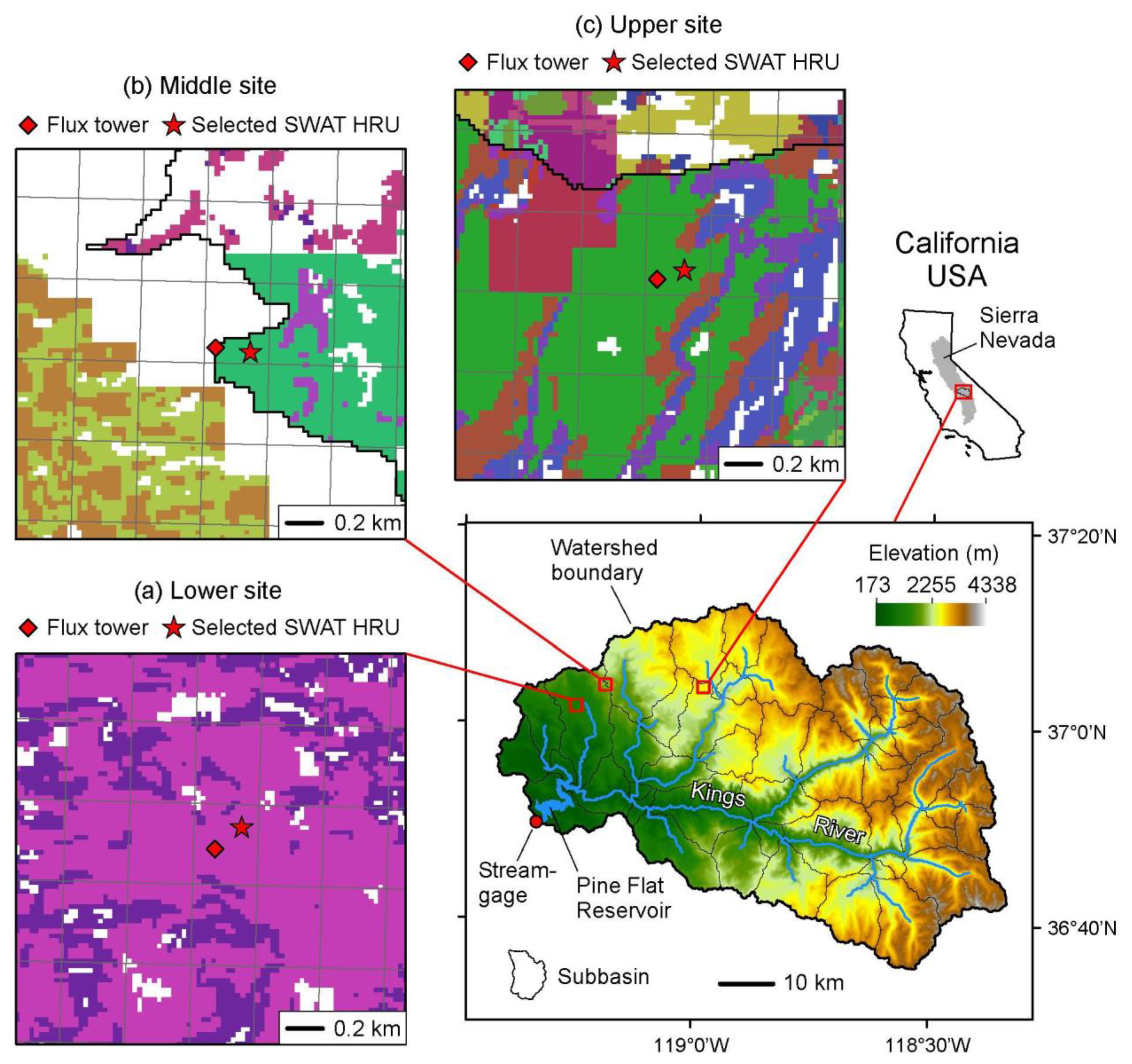
The study area is the upper Kings River watershed in the southern Sierra Nevada mountain range of California, USA. The watershed collects runoff, largely as snowmelt, from a 3999 km2 area ranging in elevation from 285 m in the western foothills to 4338 m along the Pacific Crest in the east (Figure 1, lower right). Different forks of the Kings River pass through a series of reservoirs operated for flood control and hydroelectric power (not shown) [31] to eventually empty into the Pine Flat Reservoir at the western outlet of the watershed (Figure 1, lower right). Runoff from the watershed provides water to over a million acreas of some of the world’s most fertile and productive agricultural land [31].

Figure 1.
Location of (lower right) upper Kings River watershed in southern Sierra Nevada, California, and (a–c) flux towers within watershed. In (a–c), fishnets are grid cell boundaries of the MODIS MOD16A2 ET product, and HRUs are Hydrologic Response Units of SWAT watershed model (color-shaded areas) selected for analysis based on proximity to flux tower. Topography from USGS National Elevation Dataset [32], water bodies from USGS National Hydrography Dataset [33].
The climate of the area is Mediterranean, with cool moist winters and warm dry summers. Based on 1981–2010 climatic normals from the PRISM Norm81d product [34,35], the watershed receives approximately 999 mm of precipitation per year on average, most of which (85%) occurs during the wet six-month period of November–April. A little over half of all precipitation (54%) flows out of the watershed as the Kings River based on 1981–2010 full-natural streamflow below Pine Flat Reservoir [36]. Annual precipitation in the watershed increases with elevation, from approximately 530 mm in the lowermost areas to approximately 1200 mm in the uppermost areas (Supplement Figure S1). Average air temperature is 7.1 °C at the mean elevation of 2329 m, and decreases with elevation at a rate of −5.4 °C per km (Supplement Figure S2). The phase of precipitation shifts from rain to snow with increasing elevation, becoming mostly snow at elevations above approximately 2000 m [37,38]. A little over two-thirds of the watershed (68%) resides above this rain-snow transition elevation.
Soils are distributed over approximately 59% of the watershed up to an elevation of approximately 2700 m [39,40], with exposed bedrock dominating the higher elevations. The soils grade from thermic Alfisols at lowest elevations into frigid Entisols and Inceptisols at higher elevations. These soils are loamy to sandy, well- to excessively drained, with thicknesses ranging from 20 to 250 cm [39,40]. In addition to soil, the underlying regolith (weathered bedrock) is also known to be an important source of water to vegetation [41,42]. The dominant land cover types accounting for 99% of the watershed are evergreen forest (52%), shrub/scrub (30%), barren land (rock/sand/clay) (9.8%), grassland/herbaceous (6.0%), and open water (1.4%) [43].
The watershed contains the Southern Sierra Critical Zone Observatory (SSCZO) operated in cooperation with the Kings River Experimental Watersheds program (KREW) [37,44]. This observatory includes three eddy-covariance flux towers [28], maintained by the Goulden Lab at University of California, Irvine [45], which provided the ET observations used in this study (Section 3.3). For more information about the soils, vegetation, and climate of these sites, the readers are referred to Hunsaker et al. [37], Bales et al. [38], O’Geen et al. [42], Bales et al. [44], and Safeeq and Hunsaker [46].
3. Methods
3.1. Summary
Our methods were designed to address two objectives. The first objective was to determine which would be more accurate, ET predictions from a watershed model calibrated to streamgage (ETwm) or ET predictions from a watershed model of the same area calibrated to ETrs product (rather than streamgage). We did this by comparing the ET accuracy of two models: (1) MODIS MOD16, (2) SWAT calibrated to streamgage. Model accuracies were evaluated relative to ET observations at three eddy-covariance flux towers (Figure 1). If ETrs is more accurate than ETwm, then it follows that calibrating the watershed model to that remote-sensing ET product could potentially improve the watershed model’s ET accuracy over that of a purely stream-based calibration approach. Conversely, if ETrs is less accurate than ETwm, then calibrating the watershed model to those ETrs would only degrade the watershed model’s ET accuracy relative to a stream-based calibration approach. ET observations and simulations were considered on a monthly basis during water years 2009–2018, with a water year defined to extend from October 1 through September 30. For metrics of ET model accuracy, we used the Nash-Sutcliffe efficiency (NSE) [47] which equals the fraction of variance in observations explained by a model, and model percent-bias in average ET (PBIAS) [48]. We also evaluated how well the two models producing ETrs and ETwm captured the relationship between average ET and elevation (1160–2700 m). Metrics of NSE and PBIAS were reported for the period of all water years during 2009–2018, water years with annual precipitation below the 2001–2019 median of 803 mm (“dry years”) based on PRISM AN81d product [34,35], and water years with annual precipitation at or above that median.
The second objective of this study was to compare and contrast ET from flux towers and models in a way that identifies seasonal conditions associated with model strengths and weaknesses. We started this out with an examination of monthly time series plots. Next, we compared and contrasted ET “seasonality”, defined as the set of monthly ET averages during the calendar year. Lastly, we examined relationships between monthly ET and weather variables of air temperature and vapor pressure deficit (Section 3.2), variables which influence atmospheric water demand and are also used to limit canopy conductance in the ETrs model (Section 3.4).
3.2. Weather Data
Weather data for watershed modeling and examination of ET-weather relationships were obtained from daily 2.5-arcminute PRISM AN81d product [34,35,49] and GridMET product [50]. Air temperature and vapor pressure deficit were computed from PRISM values of minimum air temperature, maximum air temperature, and dewpoint temperature, along with the equation for saturation vapor pressure in Murray [51]. Downward solar radiation and wind speed were obtained from GridMET. Daily weather time series were assembled for each subbasin of the watershed (N = 47; Figure 1, lower right) by downsampling the gridded weather data to approximately 250-m resolution, masking the downsampled data to subbasin boundaries, and computing spatial averages (Supplement section S1). These weather time series were input to ArcSWAT to force spatial elements of the watershed model referred to as Hydrologic Response Units (HRUs) (Section 3.5). The weather data used for the examination of ET-weather relationships were taken from the model HRUs nearest to the flux towers as shown in Figure 1.
3.3. Flux Tower Observations of ET
The ET observations used in this study were collected at three flux towers (Figure 1) situated along an environmental gradient ranging from rain-dominated Ponderosa pine at 1160 m to snow-dominated Lodgepole pine at 2700 m [28] (Table 1). The observations were collected during the day at 30-minute intervals using the eddy covariance method [52], at a height of 5–10 m above the tallest trees [28]. We first obtained the 30-minute ET observations and “Flexible Filler” processing script (Matlab) from the Goulden Lab [45]. Using the Flexible Filler script, we filtered out 30-minute data during calm atmospheric conditions and filled the resulting gaps using the regression approach in Goulden et al. [28,52]. The filtered, gap-filled data were then aggregated to monthly values, requiring at least 50% data availability for each month. Dates of data availability slightly differed for each flux tower, as shown in Table 1.

Table 1.
Site characteristics of eddy covariance flux towers providing ET observations for this study [28]. These sites are mapped in Figure 1. Water years of data used for this study are listed at right. Years with partial data availability, indicated with asterisk, provided less than 11 out of 12 months’ worth of data.
3.4. Remote Sensing of ET
The ETrs product used in this study was the 8-day, 0.25-arcminute global MOD16A2 product from MODIS sensors onboard the Terra and Aqua satellites [11,12,53]. The model behind this product uses a modifed Penman-Monteith approach adapted from Cleugh et al. [6] to predict evaporation from wet and dry soil, evaporation from wet canopy, and transpiration from dry canopy [12,54]. The model operates at a daily time step using meteorology from NASA’s Global Modeling and Assimilation Office (GMAO) reanalysis dataset (1.0 × 1.25° resolution), 8-day composites of absorbed photosynthetically active radiation (FPAR) and leaf area index (LAI), and 16-day composites of albedo. Limitations on ET associated with water availability and stomatal physiology (e.g., Jarvis [55]) are modeled in the MOD16A2 product using canopy conductance correction factors consisting of linear functions of vapor pressure deficit and minimum air temperature [11,12,54]. These functions are parameterized by biome-specific look-up tables organized by land cover classification (Table 3.2 of Running et al. [54]).
There was some uncertainty as to how ET in individual MODIS cells, each approximately 500-m across, would correspond to flux tower observations which collect fluxes from areas (footprints) typically measuring 100–2000 m across [56]. For the comparisons to ET from SWAT and flux towers, and in consideration of plausible intra-footprint variability in MODIS data (see Supplement Figure S3), we decided to obtain the MODIS ET data from the single MODIS cells containing the flux tower locations (Figure 1). This decision followed from the results in Supplement Figure S3 showing that MODIS intra-footprint variability tends to be substantially less than same-cell differences between MODIS and flux tower. We filtered out any MOD16A2 data having QA/QC flags not of “good quality” and not free of “significant” cloud cover, then aggregated it to monthly values using time-weighted averaging and requiring at least 50% data availability for each month.
3.5. Watershed Modeling of ET
We modeled ET in the upper Kings River using the Soil & Water Assessment Tool (SWAT) version 2012, with ArcSWAT version 2012 for model construction. SWAT dates back to the late 1970s for research into land management impacts on water, sediment, nutrients, and pesticides [57,58,59]. It has been widely used to simulate hydrologic fluxes in snow-influenced watersheds such as this study area [60,61,62,63,64,65]. In SWAT, the water conservation equation is solved at a daily time step in HRUs, each of which is a numerical 1-D element (“bucket”) of homogeneous land cover, soil, and slope. Each HRU exchanges water/energy with the atmosphere (including ET) and delivers runoff directly to the stream reach within enclosing subbasin (subbasins shown in Figure 1, lower right). We selected the Penman-Monteith option for potential ET; actual ET was computed based on potential ET and water availability in soil and underlying aquifer [66].
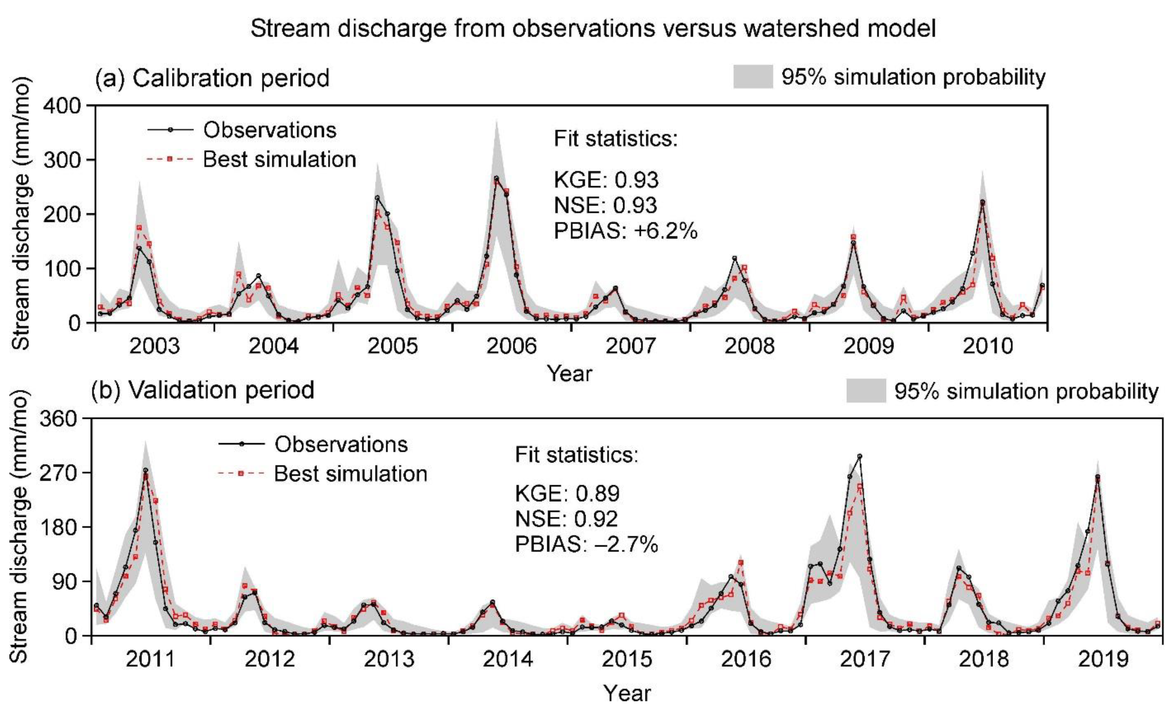
To construct the watershed model, we first built a “base model” in ArcSWAT using the parameters and input datasets for elevation, soil, land cover, meteorology, and snow cover detailed in Supplement section S1. We then initialized the base model with LAI and biomass from the end of a 30-year spin-up forced by dynamic steady-state weather (Supplement section S2), forming the “plant spin-up” model representing mature forest conditions at the start of simulations. Next, we applied a calibration procedure to the plant spin-up model as follows. First, we used a global sensitivity analysis (GSA) to identify the most influential parameters of the plant spin-up model to estimate via calibration. Using the Sobol method of GSA [67], we identified the influential parameters (N = 12) accounting for 99% of the variance in model streamflow error (Supplement section S3). Next, we calibrated the plant spin-up model by estimating values of influential parameters that minimized model errors relative to 2003–2010 monthly, full-natural streamflow at the watershed outlet [36], as described in Supplement section S4. We used for calibration the Sequential Uncertainty Fitting algorithm (SUFI-2) calibration and uncertainty tool of the SWAT-CUP software package [68,69,70]. Lastly, we validated the calibrated model to 2011–2019 monthly, full-natural streamflow using the parameter ranges obtained from calibration (Supplement Table S6). Simulations for calibration and validation were spun up to a total of 13 years of weather data, consisting of 10 years of dynamic steady-state weather (for aquifer equilibration) followed by three years of real weather (for soil and plant equilibration) (Supplement sections S2 and S4). In terms of model performance, the calibrated and validated models both showed “very good” results (Figure 2) based on criteria in Moriasi et al. [48] and Abbaspour et al. [68]. For the comparisons to flux tower and MODIS, we used monthly ET of the “best” simulation (Figure 2) taken from the HRUs nearest to the flux towers (Figure 1).
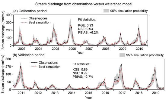
Figure 2.
Monthly stream discharge at Pine Flat Dam from observations versus best simulation of SWAT watershed model. 95% simulation probability also shown, defined at the 2.5– to 97.5–percentile of monthly simulations. Fit statistics are for “best simulation” having the highest objective function, i.e., the Kling-Gupta efficiency (KGE) [71]. NSE = Nash-Sutcliffe efficiency [47], PBIAS = model percent bias [48].
4. Results
4.1. Long-term ET
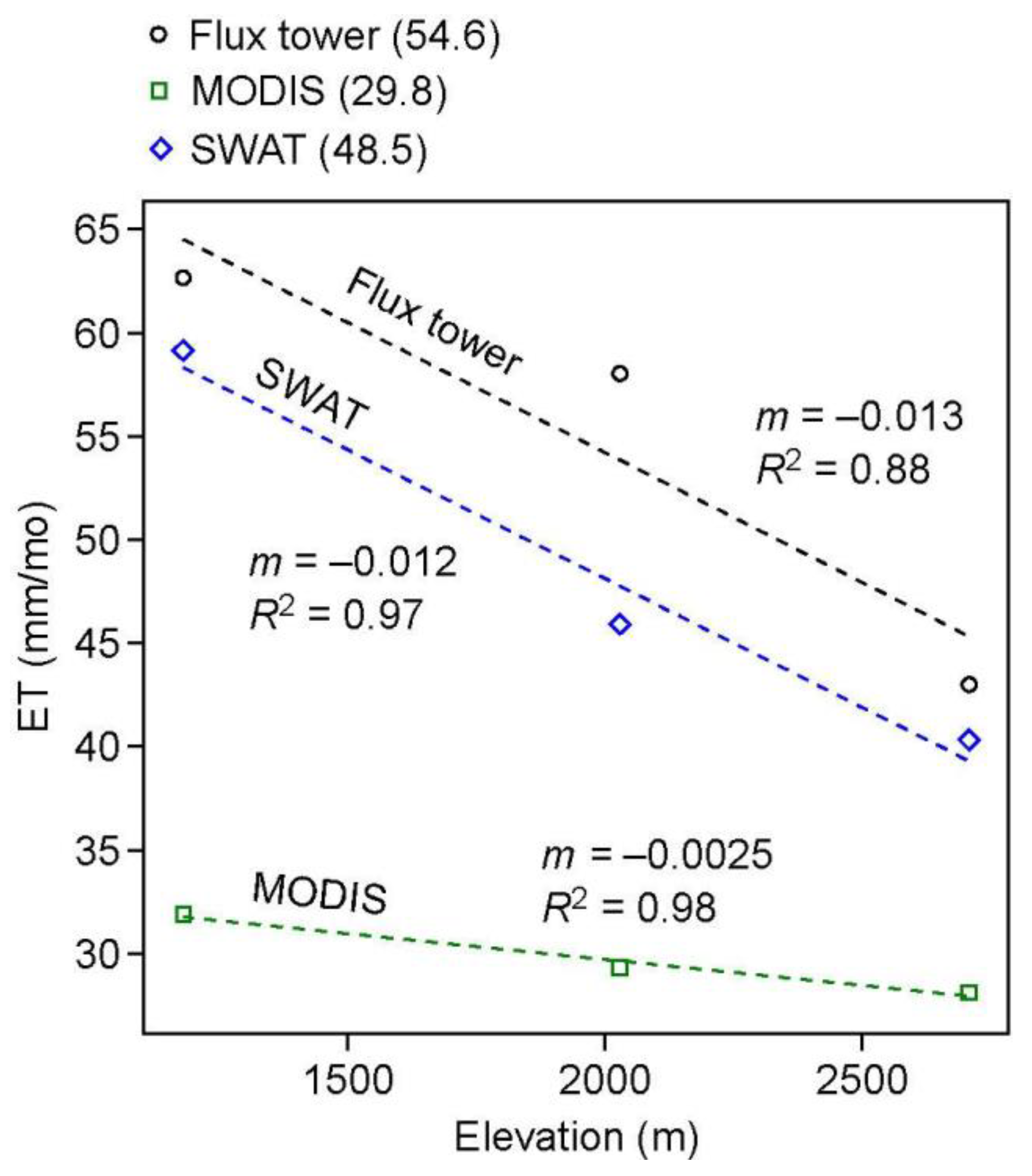
Long-term ET observations were substantially greater than the MODIS model predictions and greater but more similar to the SWAT model predictions. Observed ET averaged across all months and flux towers was 54.6 mm/mo (Figure 3). This value was 13% greater than SWAT’s prediction (48.5 mm/mo), 83% greater than MODIS’s prediction (29.8 mm/mo) (Figure 3). In addition, observed long-term ET in the upper Kings River decreased with elevation at a markedly steeper rate than the MODIS model predicted. Based on the flux tower network, ET decreased with elevation at a rate of −0.013 mm mo−1 m−1 (Figure 3). This rate was fairly close (7.7%) to the SWAT model prediction of −0.012 mm mo−1 m−1 (Figure 3). In contrast, the MODIS model predicted an elevational trend of only −0.0025 mm mo−1 m−1, one-fifth the observed value. These results showed that both magnitude and elevational trend in long-term ET were predicted much more accurately by SWAT than MODIS.

Figure 3.
Average monthly ET versus elevation from flux towers, MODIS, and SWAT. Averages across all elevations are parenthesized in the legend. m = slope of linear-regression trendline, R2 = coefficient of determination of linear-regression fit.
4.2. Monthly ET
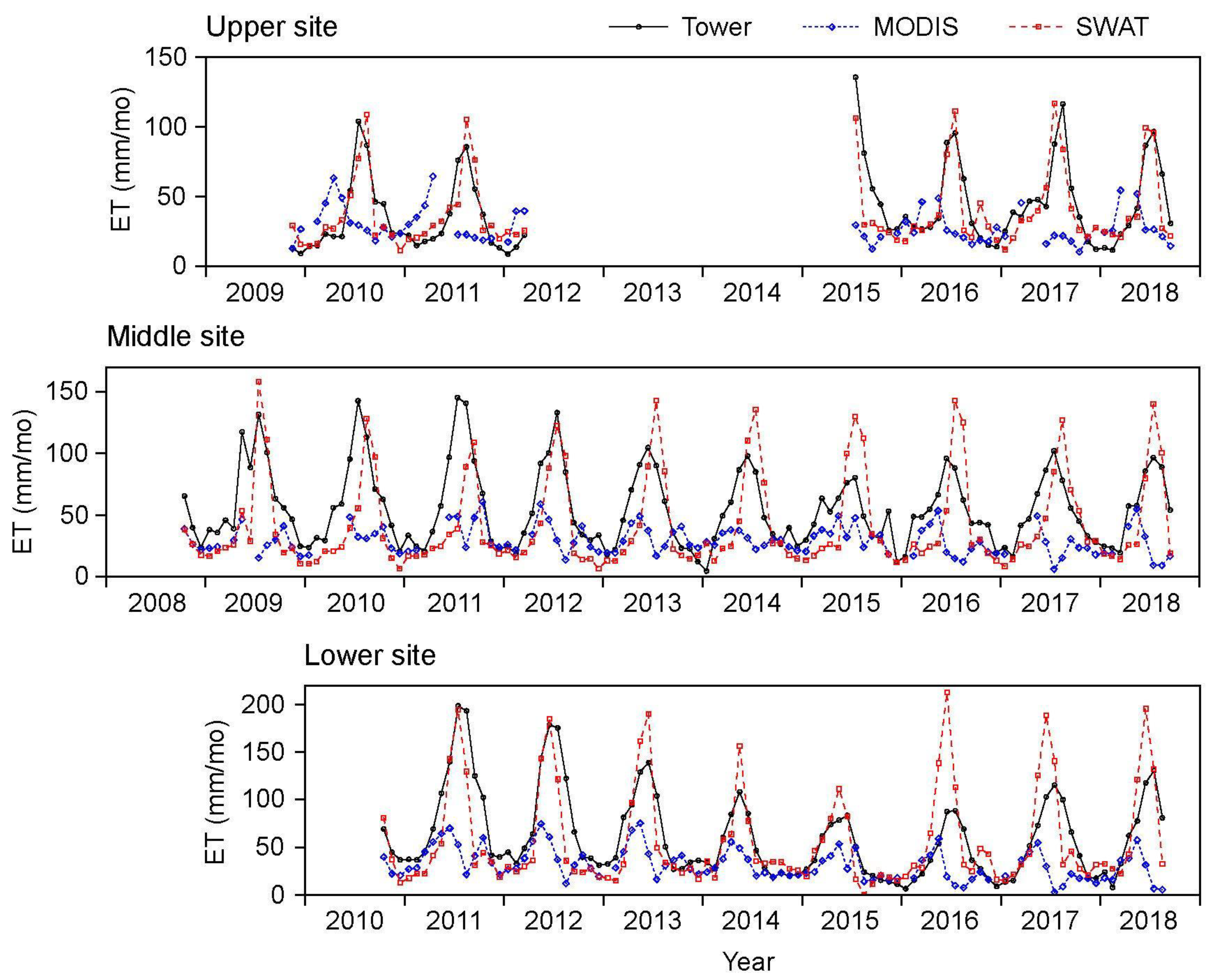
ET observations from the flux towers followed a seasonal pattern that roughly tracked the length of daylight, with peak values occurring near the middle of calendar years and minimum values occurring near the end of calendar years (Figure 4). Outputs from the SWAT model followed a similar seasonal timing, although the shape of its annual waveforms was sometimes excessively narrowed and peaked, such as in year 2016 at the middle site (Figure 4, middle). The MODIS model produced annual waveforms in ET that were notably out of phase with observations and SWAT model predictions. ET-values from MODIS tended to be on a descending limb, or near their annual minima (within one month thereof), during summer when observed and SWAT-modeled ET were near their maxima. This out-of-phase characteristic of MODIS predictions was especially apparent during years 2016–2018 at the lower and middle sites (Figure 4). In addition, the annual ET waveforms from MODIS appeared less distinct than those from observations and SWAT.
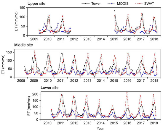
Figure 4.
Monthly ET from flux towers, MODIS, and SWAT at three sites in upper Kings River watershed.
In terms of the NSE metric of model fitness, the SWAT model matched monthly ET observations better than the MODIS model. The NSE of SWAT across all flux tower sites was +0.36, ranging from +0.04 at the middle site to +0.68 at the upper site (Table 2). In comparison, the NSE of MODIS across all sites was −0.43, ranging from −0.73 at the middle site to −0.33 at the lower site. These negative NSE-values indicate a level of prediction efficiency lower than that provided by knowledge of long-term observed ET. Both SWAT and MODIS showed minimum prediction efficiency at the middle site (Table 2). In addition, both models showed slightly lower prediction efficiency (NSE lower by ~0.2) during wet years than dry years (Table 2).

Table 2.
Error statistics of monthly ET from MODIS, SWAT, and air temperature corrected MODIS, relative to flux tower observations. “All site” statistics (bottom) are for monthly ET data concatenated across the three sites. “All years” are water years 2009–2018, “wet years” are water years 2009–2011 and 2016–2017, and “dry years” are water years 2012–2015 and 2018. NSE = Nash-Sutcliffe efficiency [47], PBIAS = percent bias (positive = model overestimate) [48], N = number of months.
In terms of model bias, both SWAT and MODIS underestimated long-term ET as shown by negative PBIAS-values in Table 2. However, the underestimates from MODIS were substantially greater in magnitude than those from SWAT. The SWAT model underestimated average monthly ET across all sites by 13% (PBIAS = −13%). These underestimates ranged from 23% at the middle site to 5% at the other two sites. In comparison, the MODIS model underestimated average monthly ET across all sites by 47% (PBIAS = −47%), with underestimates ranging from 50% at the middle site to 35% at the upper site.
4.3. Seasonality in ET and Weather
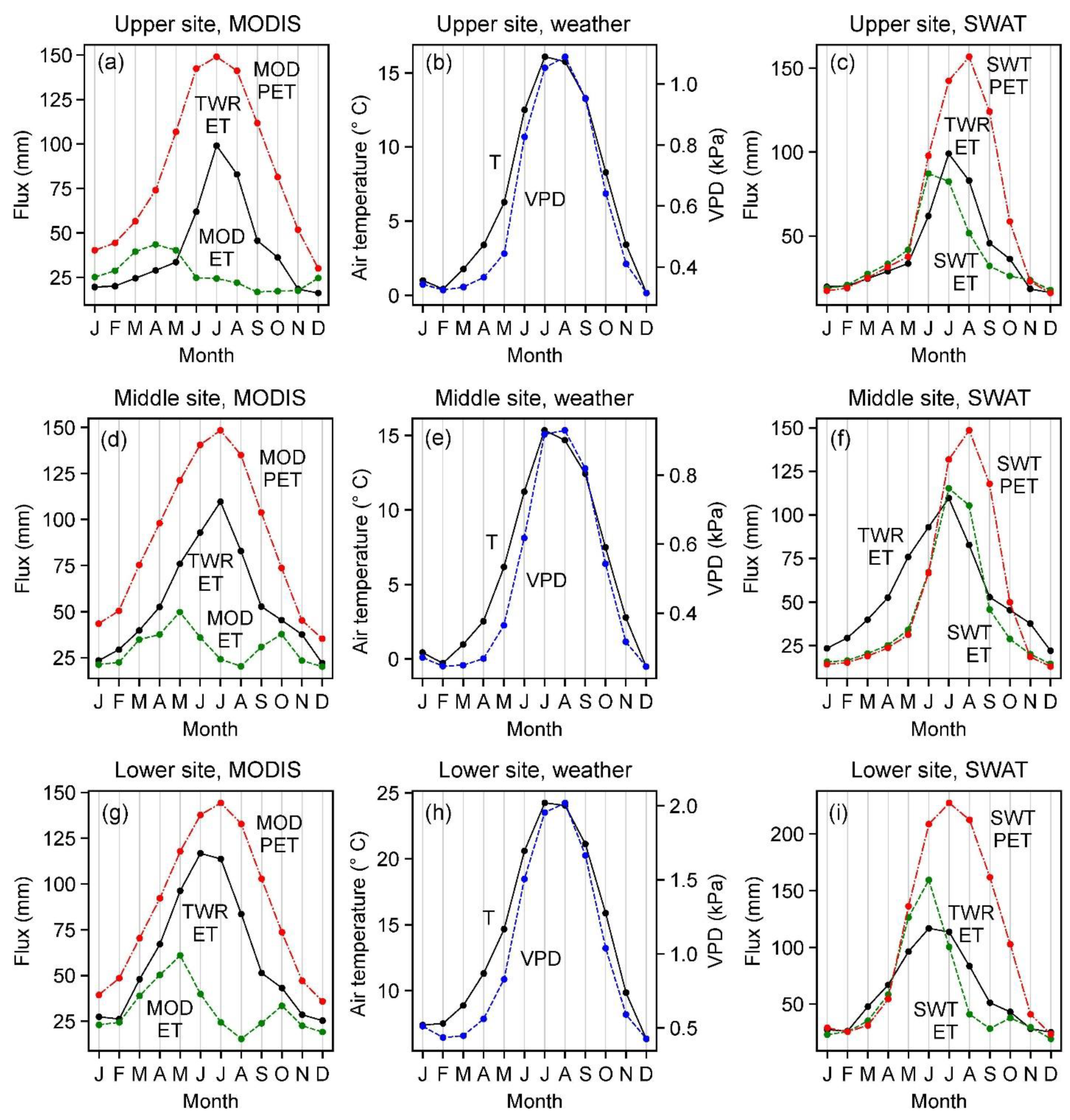
Seasonal distributions in ET, potential ET (PET), and weather variables are plotted in Figure 5. Observed ET at the flux towers reached peak values in June or July, following a seasonal distribution (“seasonal curve”) that was well aligned with PET from MODIS (Figure 5, left column). Air temperature and vapor pressure deficit reached peak values in July or August (Figure 5, middle column), following seasonal curves that closely tracked one another. This close tracking indicated a strong cross-correlation of these weather variables on a monthly time scale (R2 = 0.89–0.94 for three sites, not shown). Based on these results, air temperature and vapor pressure deficit reached maximum seasonal values within approximately one month of observed ET and MODIS PET. This timing seemed reasonable given that these weather variables are known to strongly influence atmospheric water demand.
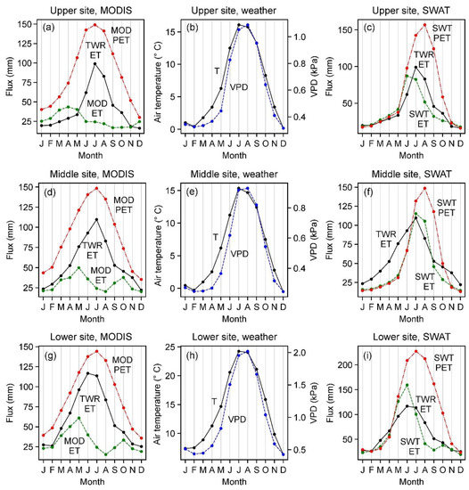
Figure 5.
Monthly averages in air temperature (T), vapor pressure deficit (VPD), ET, and potential ET (PET) at the (a–c) upper site, (d–f) middle site, and (g–i) lower site. TWR = flux tower observation, MOD = MODIS value, SWT = SWAT value. MODIS PET (MOD PET) values have been multipled by 0.5.
A seasonal asynchronicity was observed between MODIS ET and MODIS PET. MODIS ET reached a seasonal minimum only 1–2 months after the seasonal maximum in MODIS PET (Figure 5, left). MODIS PET reached a maximum value in July at all three sites. In comparison, MODIS ET reached a minimum value only one month later at the lower and middle sites, and two months later at the upper site (Figure 5, left). Such occurrences of minimum ET near the time of maximum atmospheric water demand are indicative of pronounced limitations on ET in the MODIS model.
Seasonal curves of SWAT ET tended to be skewed toward times earlier in the year relative to SWAT PET (Figure 5, right). These ET and PET curves closely tracked one another between December and mid-summer. Then, in mid-summer, the ET curves began following descending limbs 1–2 months before descending limbs of PET. This difference in timing of descending limbs produced summer and fall deficits of ET relative to PET (Figure 5, right). Such skewness of ET relative to PET is indicative of a seasonal shift in limitation on ET in the SWAT model.
4.4. ET-weather Relationships
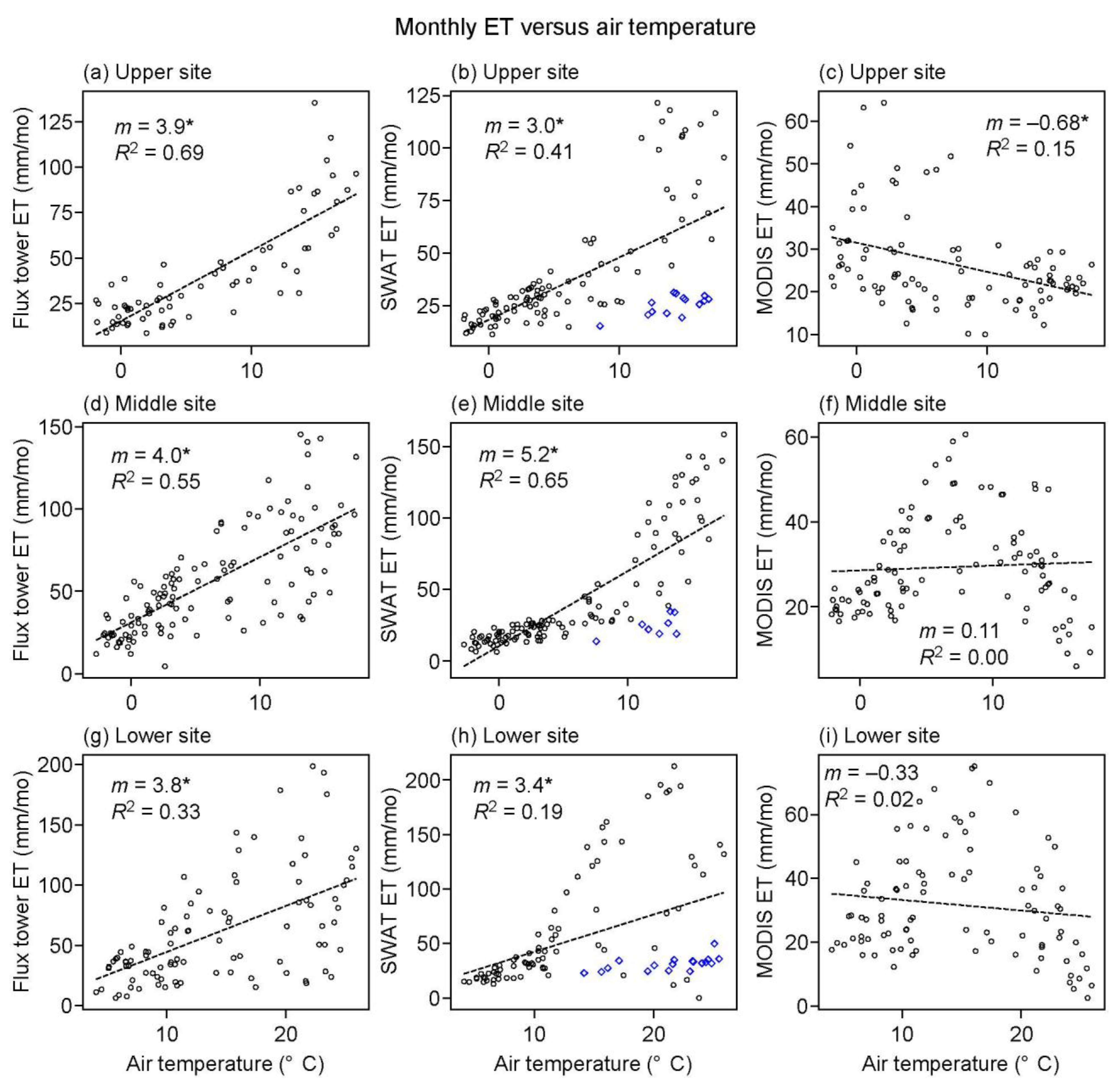
The SWAT- and MODIS-models produced markedly different relationships between monthly ET and weather. Monthly ET from SWAT, as well as flux towers, showed a significant positive relationship to air temperature (Figure 6, left and middle columns). At the flux towers, slopes of linear regression between ET and temperature ranged from 3.8 to 4.0 mm mo−1 (°C)−1. These slopes for SWAT ranged from 3.0 to 5.2 mm mo−1 (°C)−1. In contrast, monthly ET from MODIS showed either no significant relationship to temperature (p-value > 0.05) or a significant negative relationship (Figure 6, right column). At the lower and middle sites where no significant relationship to temperature occurred, there were distinct mid-temperature peaks in MODIS ET. At the lower site, MODIS ET reached a peak value at an intermediate air temperature of 16.1 °C (Figure 6i). At the middle site, this peak ET occurred at an intermediate temperature of 7.9 °C (Figure 6f). Mid-temperature ET peaks such as these did not occur in the flux tower observations or SWAT predictions. Vapor pressure deficit, noted earlier to be strongly correlated to temperature, showed a significant positive relationship to ET from both flux towers and SWAT model (Supplement Figure S6). In contrast, vapor pressure deficit showed either no significant relationship (p-value > 0.05) or a significant negative relationship to ET from MODIS (Supplement Figure S6).

Figure 6.
Monthly ET versus air temperature from different data sources at the (a–c) upper site, (d–f) middle site, and (g–i) lower site. Dashed lines are best fits from linear regression. m = slope of regression best-fit with asterisk where p-value < 0.05, R2 = coefficient of determination of best-fit. In center column, SWAT modeled ET supplied primarily by aquifer water (“revap” flux) are plotted as blue-colored diamond symbols.
Scatterplots of monthly ET from SWAT exhibited kink-like features at the middle and upper sites, and a bifurcation pattern at the lower site (Figure 6, middle column). Data points within the elbows of these kinks and lower arms of bifurcation occurred during times when SWAT ET was supplied primarily by aquifer water (blue diamond symbols in Figure 6, middle column). At other times, SWAT ET was supplied primarily by water in soil overlying the aquifer. The transition from soil- to aquifer-sourced ET was observed (not shown) to coincide with the relatively abrupt declines in SWAT ET during late summer and fall (Figure 4), and may have contributed to the excessively narrow shapes of ET annual waveforms mentioned in Section 4.2.
5. Discussion
5.1. Need to Assess Remotely Sensed ET before Use in Watershed Model Calibration
Our results illustrate a case where spatiotemporal information about ET would be represented more accurately by a watershed model calibrated to streamflow than a watershed model calibrated to ETrs. This assertion follows from our finding that the ETrs (MODIS) data were less accurate than ET predictions from watershed model calibrated to streamflow. ET from the MODIS model had a PBIAS of −47% and NSE of −0.43 across all sites, compared to a PBIAS of −13% and NSE of +0.36 for ET from the stream-calibrated watershed model (Table 2). Moreover, the negative relationship between long-term ET and elevation (Figure 3) was underestimated by 81% in the MODIS model compared to only 8% in the stream-calibrated watershed model. In general, there would clearly be cases where a watershed model’s representation of ET would likely be improved via calibration to ETrs, one example being a watershed not instrumented with any streamgages. More study is needed, however, to understand the conditions (e.g., climate, modeling frameworks, density of observations) for which the use of ETrs for watershed model calibration would produce superior ET accuracy over use of observed stream discharge.
5.2. Representation of Water Iimitation in Remote Sensing Products
Plants respond to water stress by regulating their stomata, which in turn modifies transpiration rate [8]. This regulation process is known to be a complex function of atmospheric conditions and plant water potential (including cell turgor pressure) [55,72]. The MODIS ET model accounts for this by numerically correcting the canopy conductance of water vapor using functions of minimum air temperature and vapor pressure deficit (VPD) [11,12,54]. The air temperature component of this conductance correction is meant to account for temperature limitation on plant growth while the VPD component is meant to account for water limitation. For weather at the lower site, the MODIS algorithm would predict an increase in canopy conductance with air temperature to approximately 15 °C, then a decrease in canopy conductance with further warming (Supplement Figure S7b). Below the transition temperature of 15 °C, the temperature-correction component dominates the overall correction to ET giving “temperature-limited” transpiration. Above the transition temperature, the VPD-correction component dominates giving “water-limited” transpiration. The transition temperature of 15 °C approximately coincides with the observed air temperature at which MODIS ET reaches a peak value at the lower site, 16 °C (Figure 6i). Based on this finding, the negative trend shown in Figure 6i between MODIS ET and air temperature for air temperatures > 16 °C, and absence of significant relationship between ET and temperature overall, can be explained by unrealistically high VPD-limitation on ET in the MODIS model.
This argument also seems to apply to the middle site. As a reminder, the air temperatures used in an ET-weather relationship were obtained from the watershed subbasin containing the selected site of interest (Section 3.2, Figure 1). Air temperatures at the middle site were 8 °C cooler on average than at the lower site (Figure 5e versus Figure 5h). This temperature difference exactly coincides with the −8 °C offset of maximum MODIS ET at the middle site relative to the lower site (Figure 6f versus Figure 6i). This can be explained as follows. The 8 °C difference in air temperature between the lower and middle sites occurred across a relatively short distance of approximately 7 km (Figure 1). A difference in weather across this short of distance would not be registered in the MODIS ET product because of its use of weather data at 1° × 1.25° resolution [11,12]. A mismatch in resolution of weather forcings between the SWAT model (0.042° × 0.042°) and MODIS model (1° × 1.25°) would thus introduce an apparent ET offset of −8 °C at the middle site relative to the lower site. This argument does not seem to apply at the upper site because at that location, a clear transition from temperature-limited ET to water-limited ET with increasing air temperature did not occur (Figure 6c).
Based on this interpretation, the relatively large underestimates in warm-season ET from MODIS (Figure 4 and Figure 5) stemmed from excessive VPD-limitation on canopy conductance in the MODIS model. In addition to atmospheric conditions, canopy conductance is known to be a function of plant water potential, which in turn depends on subsurface water availability and the ability of plants to access that water through their roots [72]. Weather, water availability, and plant roots are independent factors (at least to some degree), which is likely a reason for differing ET-VPD relationships across different geographic regions [73,74]. In the snow-influenced Mediterranean climate of the study area, snowmelt is known to be an important source of water to forest during the dry season. In such environments, VPD and actual water availability in the subsurface may be more loosely coupled than in the environments to which the MODIS model has been trained [75].
5.3. Regression-Based Correction to Remotely Sensed ET
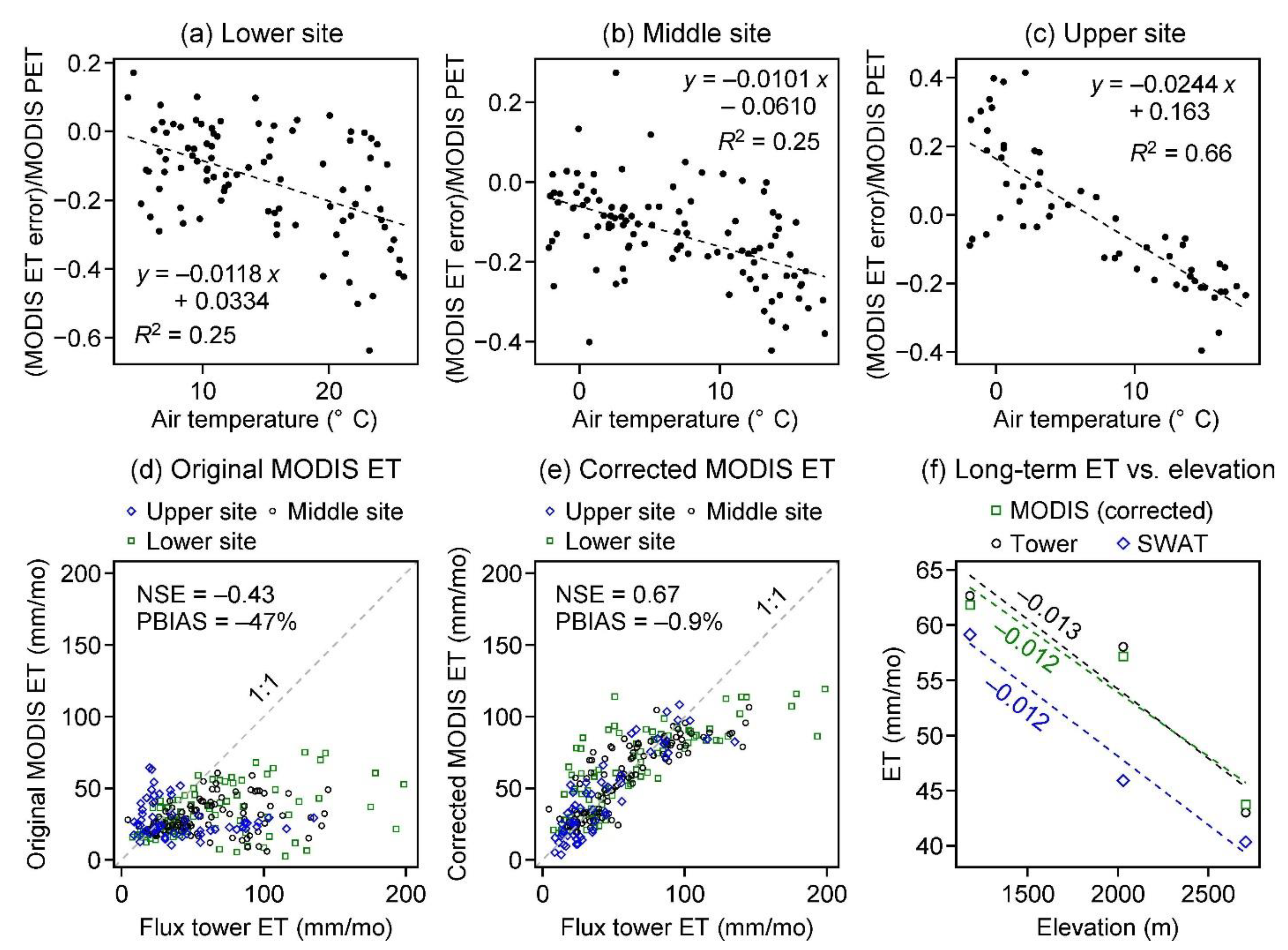
ET from observations and the MODIS model showed markedly different relationships to weather variables (Section 4.4). Correlations between ET and air temperature were significantly positive at the flux towers (Figure 6, left) and either negative or not significant from MODIS (Figure 6, right). These contrasting ET-temperature relationships provided a possible basis for correcting MODIS ET to weather using linear regression. MODIS ET error expressed as a fraction of PET, defined as yregr = (MODIS ET − flux tower ET)/(MODIS PET), was found to be well correlated to air temperature. Best fits from linear regression had slopes ranging from −0.010 to −0.024 °C−1 and R2-values of 0.25–0.66 (Figure 7a−c). The best of all fits was found at the upper site, where the R2 was 0.66 (Figure 7c). We used this regression model to predict corrected values of MODIS ET, set equal to MODIS ET − [(MODIS PET) × yregr]. The resulting predictions of corrected MODIS ET matched the flux tower observations better than both the original MODIS ET and the SWAT model (Figure 7d–f). The corrected MODIS ET had an NSE-value of +0.67 and a PBIAS of −0.9% across all sites, statistics considerably better than those of both the uncorrected MODIS model and the SWAT model (Table 2, bottom). In addition, most of the error in elevational trend in long-term MODIS ET was removed by the regression-based correction to weather (Figure 3 versus Figure 7f). The PBIAS of the corrected MODIS ET was noted to be 12% higher during dry years than wet years (Table 2, bottom), suggesting that regression models trained separately to dry and wet periods may provide further improvement to the correction method.
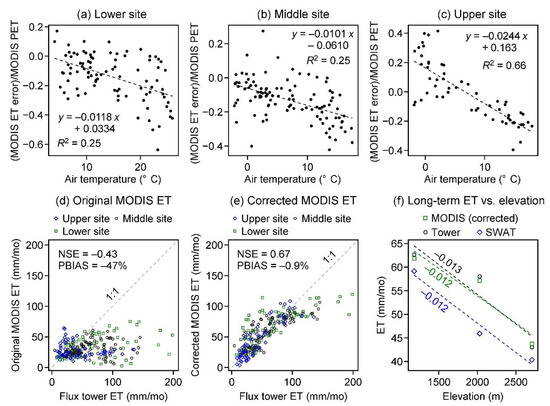
Figure 7.
Weather correction to MODIS monthly ET using linear regression with air temperature as predictor variable. (a–c) Results of linear regression between MODIS ET error, as fraction of MODIS potential ET, and monthly air temperature for each site. MODIS ET error is defined as MODIS ET—flux tower ET. (d) Original (uncorrected) MODIS ET versus flux tower ET shown with 1:1 line. (e) Weather-corrected MODIS ET versus flux tower ET. (f) Average monthly ET from weather-corrected MODIS, flux tower, and SWAT versus elevation for comparison to Figure 3. Dashed lines are trendlines from linear regression, labeled with value of slope.
6. Conclusions
The concept of using remotely sensed ET products as “observations” for watershed model calibration offers great potential for resolving spatial heterogeneity in landscape properties. However, the extent to which that numerically resolved information corresponds to actual conditions on the ground has yet to be determined. That correspondence should depend on the relative accuracies of the two models involved: (1) the model behind the remote sensing product and (2) the watershed model not calibrated to the remote sensing product. We examined this by comparing the accuracy of ET from a remote sensing product, MODIS MOD16A2, to the accuracy of ET from a watershed model (SWAT) calibrated to streamflow. ET accuracies were evaluated relative to observations from three flux towers in a Mediterranean climate extending from rain-dominated Ponderosa pine at 1160-m elevation to snow-dominated Lodgepole pine at 2700-m elevation.
The accuracy of ET from the SWAT watershed model surpassed that from the MODIS model across time and space. SWAT explained 4–68% (36% overall) of the variance in monthly ET observations at the flux towers, while MODIS explained none of the observed variance as shown by negative values of Nash-Sutcliffe efficiency. Long-term ET observed across the towers decreased with elevation at a rate of −0.013 mm mo−1 m−1. This elevational trend in long-term ET was slightly underestimated by SWAT, 7.7%, and largely underestimated by MODIS, 81%. These findings show that if the watershed model had been calibrated to remotely sensed ET rather than to stream discharge observations, the resulting accuracy of watershed model ET-predictions would have been substantially degraded.
The relatively large ET-errors from the MODIS model are interpreted to stem at least in part from an unrealistic dependence of canopy conductance on vapor pressure deficit (VPD). This interpretation is based on an erroneous reversal in slope of MODIS ET versus air temperature that approximately coincides with the transition from temperature- to VPD-controlled limitation on canopy conductance in the MODIS algorithm. This would explain the large underestimates in MODIS ET during the warmest times of the year when VPD reaches peak values. The empirical correction used in the MODIS algorithm to account for water limitation on ET may not represent the actual dynamics of water availability in the study area, which may be more loosely coupled to VPD than is assumed in the MODIS model.
Errors in monthly MODIS ET were found to be well correlated to air temperature. We showed that this could be used to “correct” ET-values from MODIS using linear regression with inputs of MODIS ET error, MODIS potential ET, and air temperature. This correction procedure removed much of the error in ET from the MODIS model, and produced ET predictions more accurate than those from the SWAT model. The regression-corrected MODIS ET may therefore serve as an improved source of “observations” for spatial calibration of a watershed model over the original MODIS ET data.
Supplementary Materials
The following are available online at https://www.mdpi.com/article/10.3390/rs13071258/s1: Section S1: Construction of base watershed model in ArcSWAT; Section S2: Watershed model initialization with LAI and biomass of mature forest; Section S3: Sensitivity analysis of influential watershed model parameters; Section S4: Watershed model calibration and validation; Table S1: Spatial datasets used in construction of watershed model in ArcSWAT 2012; Table S2: Parameter values of “base model” manually entered into tables of ArcSWAT project; Table S3: Modifications to plant database of SWAT model to more closely simulate biophysical parameters of mature Sierra Nevada forest; Table S4: SWAT model parameters varied in global sensitivity analysis using Sobol method; Table S5: Results of Sobol sensitivity analysis showing contribution of each SWAT parameter to total modeled variance in Kling-Gupta efficiency (KGE) of monthly streamflow; Table S6: Parameter ranges of calibrated SWAT model found using SWAT-CUP with the SUFI-2 (Sequential Uncertainty FItting Ver. 2) method; Figure S1: Annual precipitation versus elevation in upper Kings River watershed in 100-m elevation bins; Figure S2: Annual air temperature versus elevation in upper Kings River watershed in 100-m elevation bins; Figure S3: Range of MODIS 8-day ET-values within or touching a 500-m radius buffer around each flux tower location; Figure S4: SWAT model parameterization of snow areal depletion curve for upper Kings River watershed; Figure S5: Monthly leaf area index (LAI) and biomass from 30-year spin-up of SWAT base model to steady-state weather conditions; Figure S6: Monthly ET versus vapor pressure deficit (VPD) from different data sources at each of the three study sites; Figure S7: Weather correction to canopy conductance at the lower site based on MODIS model.
Author Contributions
Conceptualization, Methodology, Formal Analysis, Visualization, and Writing—Original Draft Preparation: S.M.J.; Investigation: S.M.J. and T.C.H.; Resources: S.M.J. and B.G.; Writing—Review and Editing: S.M.J., T.C.H. and B.G.; Supervision: T.C.H.; Project Administration: S.M.J. and T.C.H.; Funding Acquisition: T.C.H. All authors have read and agreed to the published version of the manuscript.
Funding
This work was supported by internal funding from the University of California, Merced.
Institutional Review Board Statement
Not applicable.
Informed Consent Statement
Not applicable.
Data Availability Statement
Flux tower ET observations and “Flexible Filler” processing script (Matlab) were publicly available from the Goulden Lab website, Department of Earth System Science, UC Irvine. These data could be found here: https://www.ess.uci.edu/~california/ (accessed on 24 March 2021). All other data sources were publicly available as described in the Supplementary Materials.
Acknowledgments
We thank the following individuals for their assistance with various technical matters: John T. Abatzoglou, Mike L. Goulden, Qin (Christine) Ma, Xiande Meng, Erin Mutch, and Amy Newsam. We also thank the reviewers for their helpful comments on the manuscript.
Conflicts of Interest
The authors declare no conflict of interest.
References
- Abatzoglou, J.T.; Ficklin, D.L. Climatic and Physiographic Controls of Spatial Variability in Surface Water Balance over the Contiguous United States Using the Budyko Relationship. Water Resour. Res. 2017, 53, 7630–7643. [Google Scholar] [CrossRef]
- Caracciolo, D.; Pumo, D.; Viola, F. Budyko’s Based Method for Annual Runoff Characterization across Different Climatic Areas: An Application to United States. Water Resour. Manag. 2018, 32, 3189–3202. [Google Scholar] [CrossRef]
- Anderegg, W.R.L.; Flint, A.; Huang, C.; Flint, L.; Berry, J.A.; Davis, F.W.; Sperry, J.S.; Field, C.B. Tree Mortality Predicted from Drought-Induced Vascular Damage. Nat. Geosci. 2015, 8, 367–371. [Google Scholar] [CrossRef]
- Mildrexler, D.; Yang, Z.; Cohen, W.B.; Bell, D.M. A Forest Vulnerability Index Based on Drought and High Temperatures. Remote Sens. Environ. 2016, 173, 314–325. [Google Scholar] [CrossRef]
- Young, D.J.N.; Stevens, J.T.; Earles, J.M.; Moore, J.; Ellis, A.; Jirka, A.L.; Latimer, A.M. Long-Term Climate and Competition Explain Forest Mortality Patterns under Extreme Drought. Ecol. Lett. 2017, 20, 78–86. [Google Scholar] [CrossRef]
- Cleugh, H.A.; Leuning, R.; Mu, Q.; Running, S.W. Regional Evaporation Estimates from Flux Tower and MODIS Satellite Data. Remote Sens. Environ. 2007, 106, 285–304. [Google Scholar] [CrossRef]
- Fisher, J.B.; Tu, K.P.; Baldocchi, D.D. Global Estimates of the Land–Atmosphere Water Flux Based on Monthly AVHRR and ISLSCP-II Data, Validated at 16 FLUXNET Sites. Remote Sens. Environ. 2008, 112, 901–919. [Google Scholar] [CrossRef]
- Leuning, R.; Zhang, Y.Q.; Rajaud, A.; Cleugh, H.; Tu, K. A Simple Surface Conductance Model to Estimate Regional Evaporation Using MODIS Leaf Area Index and the Penman-Monteith Equation. Water Resour. Res. 2008, 44. [Google Scholar] [CrossRef]
- Zhang, K.; Kimball, J.S.; Mu, Q.; Jones, L.A.; Goetz, S.J.; Running, S.W. Satellite Based Analysis of Northern ET Trends and Associated Changes in the Regional Water Balance from 1983 to 2005. J. Hydrol. 2009, 379, 92–110. [Google Scholar] [CrossRef]
- Glenn, E.P.; Nagler, P.L.; Huete, A.R. Vegetation Index Methods for Estimating Evapotranspiration by Remote Sensing. Surv. Geophys. 2010, 31, 531–555. [Google Scholar] [CrossRef]
- Mu, Q.; Heinsch, F.A.; Zhao, M.; Running, S.W. Development of a Global Evapotranspiration Algorithm Based on MODIS and Global Meteorology Data. Remote Sens. Environ. 2007, 111, 519–536. [Google Scholar] [CrossRef]
- Mu, Q.; Zhao, M.; Running, S.W. Improvements to a MODIS Global Terrestrial Evapotranspiration Algorithm. Remote Sens. Environ. 2011, 115, 1781–1800. [Google Scholar] [CrossRef]
- Miralles, D.G.; Holmes, T.R.H.; De Jeu, R.A.M.; Gash, J.H.; Meesters, A.G.C.A.; Dolman, A.J. Global Land-Surface Evaporation Estimated from Satellite-Based Observations. Hydrol. Earth Syst. Sci. 2011, 15, 453–469. [Google Scholar] [CrossRef]
- Wagener, T.; Gupta, H.V. Model Identification for Hydrological Forecasting under Uncertainty. Stoch. Environ. Res. Risk Assess. 2005, 19, 378–387. [Google Scholar] [CrossRef]
- Yilmaz, K.K.; Vrugt, J.A.; Gupta, H.V.; Sorooshian, S. Model Calibration in Watershed Hydrology. In Advances in Data-Based Approaches for Hydrologic Modeling and Forecasting; World Scientific: Singapore, 2010; pp. 53–105. [Google Scholar] [CrossRef]
- Lin, P.; Pan, M.; Beck, H.E.; Yang, Y.; Yamazaki, D.; Frasson, R.; David, C.H.; Durand, M.; Pavelsky, T.M.; Allen, G.H.; et al. Global Reconstruction of Naturalized River Flows at 2.94 Million Reaches. Water Resour. Res. 2019, 55, 6499–6516. [Google Scholar] [CrossRef]
- U.S. Geological Survey. Landsat Provisional Actual Evapotranspiration Science Product courtesy of the U.S. Geological Survey. Available online: https://www.usgs.gov/core-science-systems/nli/landsat/landsat-provisional-actual-evapotranspiration (accessed on 23 November 2020).
- Zhang, Y.; Chiew, F.H.S.; Zhang, L.; Li, H. Use of Remotely Sensed Actual Evapotranspiration to Improve Rainfall–Runoff Modeling in Southeast Australia. J. Hydrometeorol. 2009, 10, 969–980. [Google Scholar] [CrossRef]
- Zhang, Y.; Chiew, F.H.S.; Liu, C.; Tang, Q.; Xia, J.; Tian, J.; Kong, D.; Li, C. Can Remotely Sensed Actual Evapotranspiration Facilitate Hydrological Prediction in Ungauged Regions without Runoff Calibration? Water Resour. Res. 2020, 56. [Google Scholar] [CrossRef]
- Zou, L.; Zhan, C.; Xia, J.; Wang, T.; Gippel, C.J. Implementation of Evapotranspiration Data Assimilation with Catchment Scale Distributed Hydrological Model via an Ensemble Kalman Filter. J. Hydrol. 2017, 549, 685–702. [Google Scholar] [CrossRef]
- Wambura, F.J.; Dietrich, O.; Lischeid, G. Improving a Distributed Hydrological Model Using Evapotranspiration-Related Boundary Conditions as Additional Constraints in a Data-Scarce River Basin. Hydrol. Process. 2018, 32, 759–775. [Google Scholar] [CrossRef]
- Becker, R.; Koppa, A.; Schulz, S.; Usman, M.; aus der Beek, T.; Schüth, C. Spatially Distributed Model Calibration of a Highly Managed Hydrological System Using Remote Sensing-Derived ET Data. J. Hydrol. 2019, 577, 123944. [Google Scholar] [CrossRef]
- Gui, Z.; Liu, P.; Cheng, L.; Guo, S.; Wang, H.; Zhang, L. Improving Runoff Prediction Using Remotely Sensed Actual Evapotranspiration during Rainless Periods. J. Hydrol. Eng. 2019, 24, 04019050. [Google Scholar] [CrossRef]
- Herman, M.R.; Hernandez-Suarez, J.S.; Nejadhashemi, A.P.; Kropp, I.; Sadeghi, A.M. Evaluation of Multi- and Many-Objective Optimization Techniques to Improve the Performance of a Hydrologic Model Using Evapotranspiration Remote-Sensing Data. J. Hydrol. Eng. 2020, 25, 04020006. [Google Scholar] [CrossRef]
- Jiang, L.; Wu, H.; Tao, J.; Kimball, J.S.; Alfieri, L.; Chen, X. Satellite-Based Evapotranspiration in Hydrological Model Calibration. Remote Sens. 2020, 12, 428. [Google Scholar] [CrossRef]
- Jin, X.; Jin, Y. Calibration of a Distributed Hydrological Model in a Data-Scarce Basin Based on GLEAM Datasets. Water 2020, 12, 897. [Google Scholar] [CrossRef]
- Nesru, M.; Shetty, A.; Nagaraj, M.K. Multi-Variable Calibration of Hydrological Model in the Upper Omo-Gibe Basin, Ethiopia. Acta Geophys. 2020, 68, 537–551. [Google Scholar] [CrossRef]
- Goulden, M.L.; Anderson, R.G.; Bales, R.C.; Kelly, A.E.; Meadows, M.; Winston, G.C. Evapotranspiration along an Elevation Gradient in California’s Sierra Nevada. J. Geophys. Res. Biogeosci. 2012, 117, G03028. [Google Scholar] [CrossRef]
- Mu, Q.; Jones, L.A.; Kimball, J.S.; McDonald, K.C.; Running, S.W. Satellite Assessment of Land Surface Evapotranspiration for the Pan-Arctic Domain. Water Resour. Res. 2009, 45. [Google Scholar] [CrossRef]
- Martinec, J.; Rango, A. Merits of Statistical Criteria for the Performance of Hydrological Models. J. Am. Water Resour. Assoc. 1989, 25, 421–432. [Google Scholar] [CrossRef]
- McFarland, J.R.; Tufenkjian, C.L. The Kings River Handbook, 5th ed.; Kings River Conservation District and Kings River Water Association: Fresno, CA, USA, 2009; Available online: http://www.krcd.org/_pdf/Kings_River_Handbook_2009.pdf (accessed on 8 August 2018).
- U.S. Geological Survey. National Elevation Dataset (NED) 1 arc-second 2013 1 x 1 degree ArcGrid. Reston, VA. Available online: https://nationalmap.gov/ (accessed on 12 November 2014).
- U.S. Geological Survey. National Hydrography Dataset (NHD) Medium Resolution for California 20140718 State or Territory Shapefile. Reston, VA. Available online: https://nationalmap.gov/ (accessed on 19 February 2016).
- Daly, C.; Halbleib, M.; Smith, J.I.; Gibson, W.P.; Doggett, M.K.; Taylor, G.H.; Curtis, J.; Pasteris, P.P. Physiographically Sensitive Mapping of Climatological Temperature and Precipitation across the Conterminous United States. Int. J. Climatol. 2008, 28, 2031–2064. [Google Scholar] [CrossRef]
- PRISM Climate Data, Northwest Alliance for Computational Science and Engineering, Oregon State University, Corvallis. Available online: http://prism.oregonstate.edu (accessed on 9 October 2020).
- California Data Exchange Center (CDEC) ; California Department of Water Resources. Monthly Full Natural Streamflow of Kings River at Pine Flat Dam, Station ID KGF. Available online: http://cdec.water.ca.gov/dynamicapp/wsSensorData (accessed on 15 October 2020).
- Hunsaker, C.T.; Whitaker, T.W.; Bales, R.C. Snowmelt Runoff and Water Yield along Elevation and Temperature Gradients in California’s Southern Sierra Nevada. J. Am. Water Resour. Assoc. 2012, 48, 667–678. [Google Scholar] [CrossRef]
- Bales, R.; Stacy, E.; Safeeq, M.; Meng, X.; Meadows, M.; Oroza, C.; Conklin, M.; Glaser, S.; Wagenbrenner, J. Spatially Distributed Water-Balance and Meteorological Data from the Rain–Snow Transition, Southern Sierra Nevada, California. Earth Syst. Sci. Data 2018, 10, 1795–1805. [Google Scholar] [CrossRef]
- Natural Resources Conservation Service; U.S. Department of Agriculture. State Soil Geographic (STATSGO) Data Base: Data Use Information; Miscellaneous Publication Number 1492; Fort Worth, TX, USA. 1994. Available online: http://www.fsl.orst.edu/pnwerc/wrb/metadata/soils/statsgo.pdf (accessed on 11 March 2021).
- Web Site for Official Soil Series Descriptions and Series Classification, Natural Resources Conservation Service, U.S. Department of Agriculture. Available online: https://soilseries.sc.egov.usda.gov (accessed on 8 October 2020).
- Klos, P.Z.; Goulden, M.L.; Riebe, C.S.; Tague, C.L.; O’Geen, A.T.; Flinchum, B.A.; Safeeq, M.; Conklin, M.H.; Hart, S.C.; Berhe, A.A.; et al. Subsurface Plant-Accessible Water in Mountain Ecosystems with a Mediterranean Climate. WIREs Water 2018, 5, e1277. [Google Scholar] [CrossRef]
- O’Geen, A.; Safeeq, M.; Wagenbrenner, J.; Stacy, E.; Hartsough, P.; Devine, S.; Tian, Z.; Ferrell, R.; Goulden, M.; Hopmans, J.W.; et al. Southern Sierra Critical Zone Observatory and Kings River Experimental Watersheds: A Synthesis of Measurements, New Insights, and Future Directions. Vadose Zone J. 2018, 17, 180081. [Google Scholar] [CrossRef]
- U.S. Geological Survey. NLCD 2011 Land Cover Conterminous United States. Sioux Falls, SD. Available online: https://www.mrlc.gov/ (accessed on 7 April 2020).
- Bales, R.C.; Hopmans, J.W.; O’Geen, A.T.; Meadows, M.; Hartsough, P.C.; Kirchner, P.; Hunsaker, C.T.; Beaudette, D. Soil Moisture Response to Snowmelt and Rainfall in a Sierra Nevada Mixed-Conifer Forest. Vadose Zone J. 2011, 10, 786–799. [Google Scholar] [CrossRef]
- Data Access Page: Measurement of Energy, Carbon and Water Exchange Along California Climate Gradients, Goulden Lab, Department of Earth System Science, University of California, Irvine. Available online: https://www.ess.uci.edu/~california/ (accessed on 12 December 2019).
- Safeeq, M.; Hunsaker, C.T. Characterizing Runoff and Water Yield for Headwater Catchments in the Southern Sierra Nevada. J. Am. Water Resour. Assoc. 2016, 52, 1327–1346. [Google Scholar] [CrossRef]
- Nash, J.E.; Sutcliffe, J.V. River flow forecasting through conceptual models: Part 1. A discussion of principles. J. Hydrol. 1970, 10, 282–290. [Google Scholar] [CrossRef]
- Moriasi, D.N.; Arnold, J.G.; Van Liew, M.W.; Bingner, R.L.; Harmel, R.D.; Veith, T.L. Model Evaluation Guidelines for Systematic Quantification of Accuracy in Watershed Simulations. Trans. ASABE 2007, 50, 885–900. [Google Scholar] [CrossRef]
- Daly, C.; Smith, J.I.; Olson, K.V. Mapping Atmospheric Moisture Climatologies across the Conterminous United States. PLoS ONE 2015, 10, e0141140. [Google Scholar] [CrossRef]
- Abatzoglou, J.T. Development of Gridded Surface Meteorological Data for Ecological Applications and Modelling. Int. J. Climatol. 2013, 33, 121–131. [Google Scholar] [CrossRef]
- Murray, F.W. On the Computation of Saturation Vapor Pressure. J. Appl. Meteorol. 1967, 6, 203–204. [Google Scholar] [CrossRef]
- Goulden, M.L.; Munger, J.W.; Fan, S.-M.; Daube, B.C.; Wofsy, S.C. Measurements of Carbon Sequestration by Long-Term Eddy Covariance: Methods and a Critical Evaluation of Accuracy. Glob. Change Biol. 1996, 2, 169–182. [Google Scholar] [CrossRef]
- Running, S.; Mu, Q.; Zhao, M. MOD16A2 MODIS/Terra Net Evapotranspiration 8-Day L4 Global 500m SIN Grid V006. Distributed by NASA EOSDIS Land Processes DAAC. 2017. Available online: https://doi.org/10.5067/MODIS/MOD16A2.006 (accessed on 26 August 2019).
- Running, S.W.; Mu, Q.; Zhao, M.; Moreno, A. User’s Guide: MODIS Global Terrestrial Evapotranspiration (ET) Product (MOD16A2/A3 and Year-End Gap-Filled MOD16A2GF/A3GF) NASA Earth Observing System MODIS Land Algorithm (For Collection 6); User’s Guide Version 2.1; Land Processes Distributed Active Archive Center (LP DAAC), 2019. Available online: https://lpdaac.usgs.gov/documents/378/MOD16_User_Guide_V6.pdf (accessed on 15 August 2019).
- Jarvis, J.G. The Interpretation of the Variations in Leaf Water Potential and Stomatal Conductance Found in Canopies in the Field. Philos. Trans. R. Soc. Lond. B Biol. Sci. 1976, 273, 593–610. [Google Scholar] [CrossRef]
- Baldocchi, D.; Falge, E.; Gu, L.; Olson, R.; Hollinger, D.; Running, S.; Anthoni, P.; Bernhofer, C.; Davis, K.; Evans, R.; et al. FLUXNET: A New Tool to Study the Temporal and Spatial Variability of Ecosystem–Scale Carbon Dioxide, Water Vapor, and Energy Flux Densities. Bull. Am. Meteorol. Soc. 2001, 82, 2415–2434. [Google Scholar] [CrossRef]
- Srinivasan, R.; Arnold, J.G. Integration of a Basin-Scale Water Quality Model with GIS. J. Am. Water Resour. Assoc. 1994, 30, 453–462. [Google Scholar] [CrossRef]
- Arnold, J.G.; Srinivasan, R.; Muttiah, R.S.; Williams, J.R. Large Area Hydrologic Modeling and Assessment Part I: Model Development. J. Am. Water Resour. Assoc. 1998, 34, 73–89. [Google Scholar] [CrossRef]
- Gassman, P.W.; Reyes, M.R.; Green, C.H.; Arnold, J.G. The Soil and Water Assessment Tool: Historical Development, Applications, and Future Research Directions. Trans. ASABE 2007, 50, 1211–1250. [Google Scholar] [CrossRef]
- Fontaine, T.A.; Cruickshank, T.S.; Arnold, J.G.; Hotchkiss, R.H. Development of a Snowfall–Snowmelt Routine for Mountainous Terrain for the Soil Water Assessment Tool (SWAT). J. Hydrol. 2002, 262, 209–223. [Google Scholar] [CrossRef]
- Ahl, R.S.; Woods, S.W.; Zuuring, H.R. Hydrologic Calibration and Validation of SWAT in a Snow-Dominated Rocky Mountain Watershed, Montana, U.S.A. J. Am. Water Resour. Assoc. 2008, 44, 1411–1430. [Google Scholar] [CrossRef]
- Zhang, X.; Srinivasan, R.; Debele, B.; Hao, F. Runoff Simulation of the Headwaters of the Yellow River Using the SWAT Model with Three Snowmelt Algorithms. J. Am. Water Resour. Assoc. 2008, 44, 48–61. [Google Scholar] [CrossRef]
- Ficklin, D.L.; Stewart, I.T.; Maurer, E.P. Climate Change Impacts on Streamflow and Subbasin-Scale Hydrology in the Upper Colorado River Basin. PLoS ONE 2013, 8, e71297. [Google Scholar] [CrossRef]
- Watson, B.M.; Putz, G. Comparison of Temperature-Index Snowmelt Models for Use within an Operational Water Quality Model. J. Environ. Qual. 2014, 43, 199–207. [Google Scholar] [CrossRef] [PubMed]
- Grusson, Y.; Sun, X.; Gascoin, S.; Sauvage, S.; Raghavan, S.; Anctil, F.; Sáchez-Pérez, J.-M. Assessing the Capability of the SWAT Model to Simulate Snow, Snow Melt and Streamflow Dynamics over an Alpine Watershed. J. Hydrol. 2015, 531, 574–588. [Google Scholar] [CrossRef]
- Neitsch, S.L.; Arnold, J.G.; Kiniry, J.R.; Williams, J.R. Soil and Water Assessment Tool Theoretical Documentation Version 2009; Technical Report 406; Texas Water Resources Institute: College Station, TX, USA, 2011; p. 618. Available online: https://swat.tamu.edu/media/99192/swat2009-theory.pdf (accessed on 11 April 2019).
- Chan, K.; Tarantola, S.; Saltelli, A.; Sobol’, I.M. Variance-Based Methods. In Sensitivity Analysis; Wiley: Chichester, NY, USA, 2000; pp. 167–197. [Google Scholar]
- Abbaspour, K.C.; Yang, J.; Maximov, I.; Siber, R.; Bogner, K.; Mieleitner, J.; Zobrist, J.; Srinivasan, R. Modelling Hydrology and Water Quality in the Pre-Alpine/Alpine Thur Watershed Using SWAT. J. Hydrol. 2007, 333, 413–430. [Google Scholar] [CrossRef]
- Yang, J.; Reichert, P.; Abbaspour, K.C.; Xia, J.; Yang, H. Comparing Uncertainty Analysis Techniques for a SWAT Application to the Chaohe Basin in China. J. Hydrol. 2008, 358, 1–23. [Google Scholar] [CrossRef]
- Arnold, J.G.; Moriasi, D.N.; Gassman, P.W.; Abbaspour, K.C.; White, M.J.; Srinivasan, R.; Santhi, C.; Harmel, R.D.; van Griensven, A.; Van Liew, M.W.; et al. SWAT: Model Use, Calibration, and Validation. Trans. ASABE 2012, 55, 1491–1508. [Google Scholar] [CrossRef]
- Gupta, H.V.; Kling, H.; Yilmaz, K.K.; Martinez, G.F. Decomposition of the Mean Squared Error and NSE Performance Criteria: Implications for Improving Hydrological Modelling. J. Hydrol. 2009, 377, 80–91. [Google Scholar] [CrossRef]
- Porporato, A.; Laio, F.; Ridolfi, L.; Rodriguez-Iturbe, I. Plants in Water-Controlled Ecosystems: Active Role in Hydrologic Processes and Response to Water Stress: III. Vegetation Water Stress. Adv. Water Resour. 2001, 24, 725–744. [Google Scholar] [CrossRef]
- Novick, K.A.; Ficklin, D.L.; Stoy, P.C.; Williams, C.A.; Bohrer, G.; Oishi, A.C.; Papuga, S.A.; Blanken, P.D.; Noormets, A.; Sulman, B.N.; et al. The Increasing Importance of Atmospheric Demand for Ecosystem Water and Carbon Fluxes. Nat. Clim. Change 2016, 6, 1023–1027. [Google Scholar] [CrossRef]
- Massmann, A.; Gentine, P.; Lin, C.J. When Does Vapor Pressure Deficit Drive or Reduce Evapotranspiration? J. Adv. Model. Earth Syst. 2019, 11, 3305–3320. [Google Scholar] [CrossRef] [PubMed]
- He, M.; Kimball, J.S.; Yi, Y.; Running, S.W.; Guan, K.; Moreno, A.; Wu, X.; Maneta, M. Satellite Data-Driven Modeling of Field Scale Evapotranspiration in Croplands Using the MOD16 Algorithm Framework. Remote Sens. Environ. 2019, 230, 111201. [Google Scholar] [CrossRef]
Publisher’s Note: MDPI stays neutral with regard to jurisdictional claims in published maps and institutional affiliations. |
© 2021 by the authors. Licensee MDPI, Basel, Switzerland. This article is an open access article distributed under the terms and conditions of the Creative Commons Attribution (CC BY) license (http://creativecommons.org/licenses/by/4.0/).

