Article

Impending Hydrological Regime of Lhasa River as Subjected to Hydraulic Interventions—A SWAT Model Manifestation

State Key Laboratory of Water Resources and Hydropower Engineering Science, Wuhan University, Wuhan 430072, China
*
Author to whom correspondence should be addressed.
Remote Sens. 2021, 13(7), 1382; https://doi.org/10.3390/rs13071382
Submission received: 4 February 2021 / Revised: 13 March 2021 / Accepted: 31 March 2021 / Published: 3 April 2021

Abstract

:
The damming of rivers has altered their hydrological regimes. The current study evaluated the impacts of major hydrological interventions of the Zhikong and Pangduo hydropower dams on the Lhasa River, which was exposed in the form of break and change points during the double-mass curve analysis. The coefficient of variability (CV) for the hydro-meteorological variables revealed an enhanced climate change phenomena in the Lhasa River Basin (LRB), where the Lhasa River (LR) discharge varied at a stupendous magnitude from 2000 to 2016. The Mann–Kendall trend and Sen’s slope estimator supported aggravated hydro-meteorological changes in LRB, as the rainfall and LR discharge were found to have been significantly decreasing while temperature was increasing from 2000 to 2016. The Sen’s slope had a largest decrease for LR discharge in relation to the rainfall and temperature, revealing that along with climatic phenomena, additional phenomena are controlling the hydrological regime of the LR. Reservoir functioning in the LR is altering the LR discharge. The Soil and Water Assessment Tool (SWAT) modeling of LR discharge under the reservoir’s influence performed well in terms of coefficient of determination (R2), Nash–Sutcliffe coefficient (NSE), and percent bias (PBIAS). Thus, simulation-based LR discharge could substitute observed LR discharge to help with hydrological data scarcity stress in the LRB. The simulated–observed approach was used to predict future LR discharge for the time span of 2017–2025 using a seasonal AutoRegressive Integrated Moving Average (ARIMA) model. The predicted simulation-based and observation-based discharge were closely correlated and found to decrease from 2017 to 2025. This calls for an efficient water resource planning and management policy for the area. The findings of this study can be applied in similar catchments.

1. Introduction

Dams are intended to offer substantial aid to humankind by ensuring an enhanced water availability for municipal, industrial, and agricultural uses, as well as increased capability of flood regulation and hydropower generation [1]. On the other hand, the construction of dams has considerably changed the natural flow regime of rivers worldwide. Above half of the 292 large river systems in the world have been affected by dams [2,3]. The influence of human activities in altering river discharge has profoundly increased in recent decades [4]. Over an intermediate time scale (e.g., decadal scale), human interferences in terms of water consumption, land-use change, dam construction, and sand mining, among others, are the powerful factors that escalate basin-scale hydrological changes. Therefore, a site-specific study is needed to disclose the governing effects of human disruptions on these hydrological changes [5,6,7].
To temper river floods, reduce water collection for irrigation, hydropower generation and facilitate navigation, dams have been created across big rivers around the world [8]. Dams have grown to one of the most perturbing human intrusions in river systems as the number of dams and the total storage capacity of reservoirs rapidly increase [4]. Therefore, knowledge of dam construction and its regulating effects on river discharge is crucial for river and delta management and restoration. Highly regulated rivers in China are subject to large-scale ecosystem amendments made by hydrological alterations. Many of the earlier studies related to dam-induced hydrological alterations across river basins in China focused on the impacts of large dams that generally aim to control floods in large basins, such as the Lancang River [9], the Mekong River [10], the Pearl River [11], the Yangtze River [12], and the Yellow River [13,14]. In addition to large dams, the development of small dams has also been highlighted in national energy policies in China [
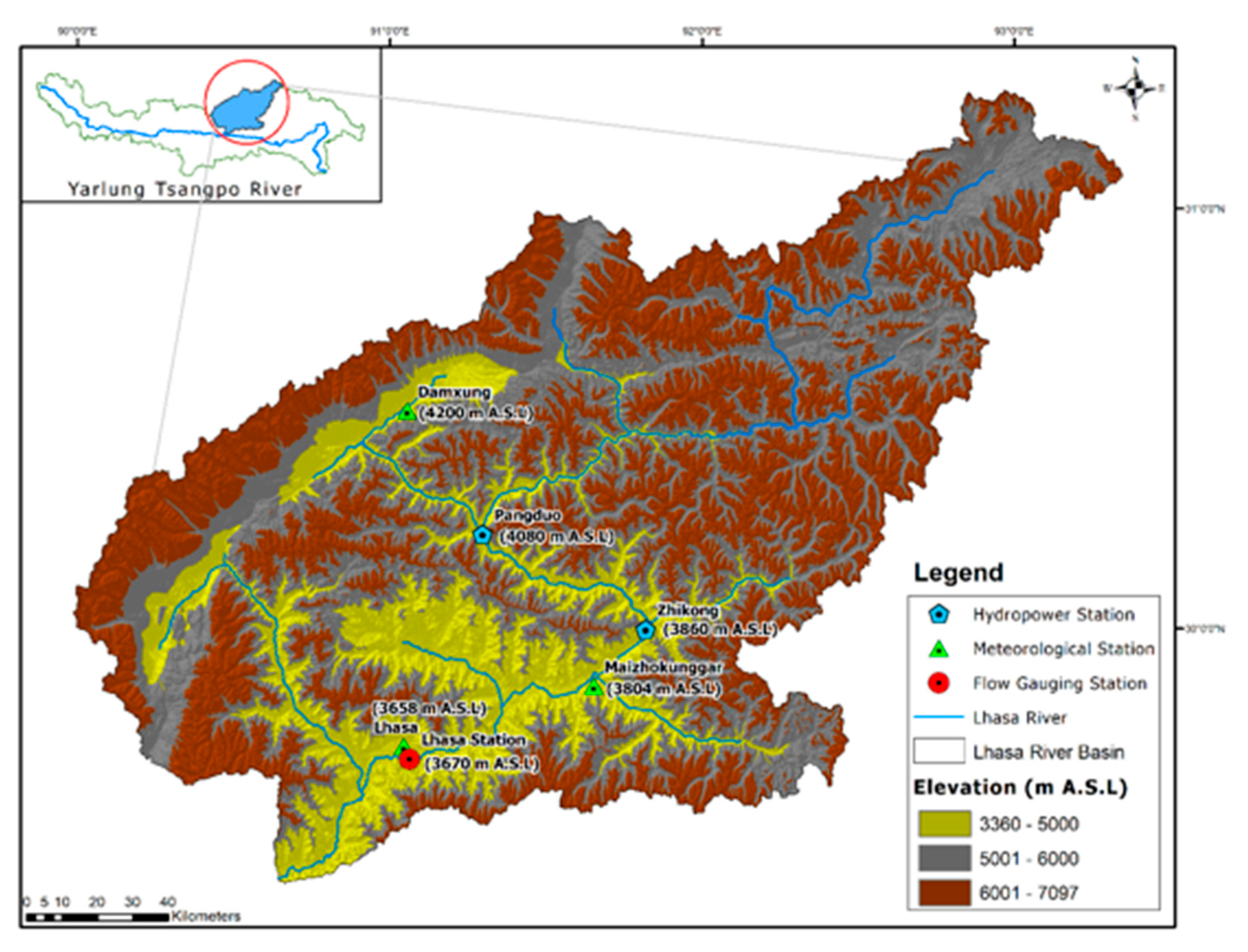
15]. Therefore, small dam construction is intense in China, especially in South China, where hydropower resources are extensive. Thus, to fill in the knowledge void, the present study focused on the impact appraisal of reservoir functioning in the Lhasa River Basin, a Qinghai–Tibetan Plateau basin in South China (for more information, see Section 2.2). Several researchers have established a number of approaches with the objective of reckoning of the hydrologic modifications caused by human activity. However, hydrological modeling can be an effective alternative for hydrological analysis in different scenarios [16]. The SWAT (Soil and Water Assessment Tool) model developed by the authors of [17] has already been in widespread use for water resource management in many different rivers [18,19,20,21,22,23]. Additionally, there has been a general lack of applications of physically-based hydrological models to the Yarlung Tsangbo River Basin, especially the Lhasa River Basin [24]. The SWAT model was applied to the Lhasa River Basin in a recent study [25], where streamflow and sediment load were predicted for the Lhasa River in future. The SWAT model was applied to the Lhasa River Basin to simulate its streamflow variability under reservoir influence [26]. The SWAT model was utilized in [27] for hydrological drought propagation in the South China Dongjiang River Basin using the “simulated–observed approach”. Their study estimated the effects of human regulations on hydrological drought from the perspective of the development and recovery processes using the SWAT model.
Streamflow forecasting is of great significance to water resource management and planning. Medium-to-long-term forecasting including weekly, monthly, seasonal, and even annual time scales is predominantly beneficial in reservoir operations and irrigation management, as well as the institutional and legal features of water resource management and planning. Due to their reputation, a large number of forecasting models have been developed for streamflow forecasting, including concept-based, process-driven models such as the low flow recession model, rainfall–runoff models, and statistics-based data-driven models such as regression models, time series models, artificial neural network models, fuzzy logic models, and the nearest neighbor model [28]. Of various streamflow forecasting methods, time series analysis has been most widely used in the previous decades because of its forecasting capability, inclusion of richer information, and more systematic way of building models in three modeling stages (identification, estimation, and diagnostic check), as standardized by Box and Jenkins (1976) [29]. The current study made use of "simulated–observed approach" after [27] for predicting the Lhasa River streamflow under reservoir operations in the Lhasa River Basin. SWAT-simulated and observed hydrological time series were used introduced to a stochastic AutoRegressive Integrated Moving Average (ARIMA) model. As a common data-driven method, the ARIMA model has been widely used in time series prediction due to its simplicity and effectiveness [30]. Adhikary et al. (2012) [31] used seasonal ARIMA (SARIMA) model to model a groundwater table. They took weekly time series and concluded that SARIMA stochastic models can be applied for ground water level variations. Valipour et al. (2013) [32] modeled the inflow of the Dez dam reservoir with SARIMA and ARMIA stochastic models. His research results showed that the SARIMA model yielded better results than the ARIMA model. Ahlert and Mehta (1981) [33] analyzed the stochastic process of flow data for the Delaware River by the ARIMA model. Yurekli et al. (2005) [34] applied SARIMA stochastic models to model the monthly streamflow data of the Kelkit River. Modarres and Ouarda (2013) [35] demonstrated the heteroscedasticity of streamflow time series with the ARIMA model in comparison to GARCH (Generalized Autoregressive Conditionally Heteroscedastic) models. Their results showed that ARIMA models performed better than GARCH models. Ahmad et al. (2001) [36] used the ARIMA model to analyze water quality data. Kurunç et al. (2005) [37] used the ARIMA and Thomas Fiering stochastic approach to forecast streamflow data of the Yesilurmah River. Tayyab et al. (2016) [38] used an auto regressive model in comparison to neural networks to predict streamflow.
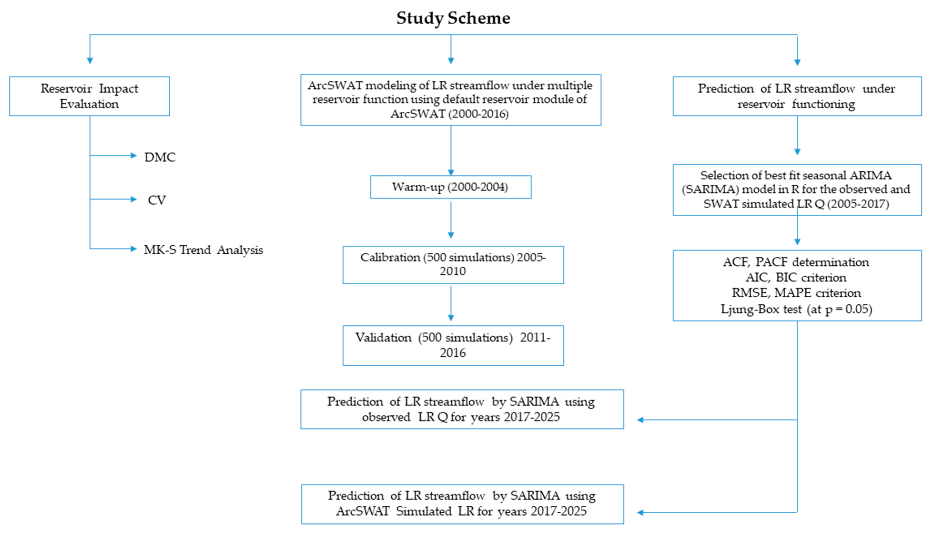
The current study primarily aimed to (i) investigate the reservoir operations’ impact on the Lhasa River discharge, (ii) apply the SWAT model to simulate Lhasa River streamflow under multiple reservoir functioning, and (iii) to predict Lhasa River streamflow under reservoir’s influence using ‘observed’ and ‘SWAT-simulated’ hydrological data series as a step forward in overcoming the data scarcity problem of the area. The study was intended to benefit water resource managers and hydrological engineers in understanding the future hydrological regime in the Lhasa River Basin under reservoir functioning and aiding in developing better management practices and planning for hydrological resources in the area. The current study holds novelty in combining a physical-based hydrological model and a statistical time series forecasting model for the simulation and prediction, of the discharge of the Lhasa River respectively, one of the important rivers in the data-scarce Qinghai–Tibetan Plateau, which is under the influence of recent major hydraulic interventions in the form of the Zhikong and Pangduo hydropower reservoirs.

2. Materials and Methods

2.1. Study Area—Lhasa River Basin

The Lhasa River Basin (LRB), ranging from 29°19′ to 31°15′N and from 90°60′ to 93°20′E, is the economical and authoritative hub of the autonomous Qinghai–Tibetan plateau (QTP). The Lhasa River (LR) is the longest tributary of the Yarlung Tsangpo River; LRB covers a ≈32,321 km2 basin area (ArcSWAT-estimated area by the digital elevation model used in the current study), comprising 13.5% of the total area of the Yarlung Tsangpo basin [39]. The LRB exhibits typical semi-arid monsoonal climate conditions, where the major proportion of received rainfall is concentrated in the summer season from June to September with the simultaneous generation of peak LR discharge during the same time. Peng et al. (2015) [24] showed that rainfall in summer is a governing feature in producing summer stream flow in the Lhasa River basin. Thus, the rainfall disproportion poses a direct influence on the rainfall-dependent runoff generation phenomena in the basin. The hydrometric and meteorological records for the LRB are maintained at the Pondo, Tanggya, and Lhasa hydrometric stations and the Damxung, Maizhokunggar, and Lhasa meteorological stations, respectively.
The LR stretches to a length of 551 km with a hydropower potential of 1.177 million kWh [39], and it is substantial in fulfilling the hydropower and agricultural requirements of the local community. The LR has been exposed to major hydraulic interventions in the form of reservoir development and confinement during the last and present decades. It is of vital importance to understand the hydrological phenomena of the LRB under the influence of hydraulic structures for a better understanding of the hydrological behavior of the study area to facilitate the understanding of future water resource availability and management in the area. The major hydraulic developments in the study area are the installation of Zhikong and Pangduo hydropower stations over the LR.

Zhikong and Pangduo Reservoirs Impoundment on Lhasa River

The Zhikong and Pangduo Dams were built in 2006 and 2013, respectively, on the LR. The Zhikong Dam is located 96 km upstream the urban Lhasa city in the middle and lower reaches of the LR, and it is 65 km downstream the Pangduo Dam, thus impounding the upper LR. To meet the substantially increasing power demand of the Tibet plateau, the Zhikong Dam was built with an installed power capacity of 100 MW and a reservoir water storage capacity of 0.225 billion m3. The other purposes of this installation include flood control in high rainfall months and irrigation water supply in low rainfall spells during the year. However, Wu et al. (2018) [39] showed that impoundment by the Zhikong Dam unswervingly altered the hydrological behavior of the downstream channels of the LR. The succeeding major hydrological intervention on the LR was the construction of the Pangduo Dam with 160 MW of installed capacity and 1.23 billion m3 of reservoir water storage capacity. The development purposes of the Pangduo water conservancy project include irrigation water availability, power generation, and flood control. It is the pillar project and a leading reservoir developed for the enormous growth of the LRB.

2.2. Datasets Used

The current study utilized an arrangement of hydro-meteorological and geospatial information of the LRB in order to establish the desired results. The datasets included the following.

2.2.1. Geospatial Data of LRB

To extract the topographical features of the LRB, a 90 m resolution Advanced Thermal Emission and Reflection Radiometer, Global Digital Elevation Model (ASTER, GDEM) was developed for the study area (Figure 1). The land use features of the LRB were established using Landsat-8 Operational Land Imager (OLI) imagery with a 30 m resolution. The best cloud free images, with (137, 39) and (138, 39) path and row respectively, were used to delineate the land use map for the study area using maximum likelihood classification of the land features. The soil profile of the LRB was described using FAO-UNESCO (Food and Agricultural Organization-United Nations Educational, Scientific, and Cultural Organization) Harmonized World Soil Database version 1.2 (HWSD v1.2), a 30 arc-second raster database with over 15,000 different soil mapping units within the 1:5,000,000 scale FAO-UNESCO Soil Map of the World. All the datasets were projected to Universal Transverse Mercator 45N projection. All these datasets were mandatory input for SWAT model to simulate the LR streamflow.

2.2.2. Hydro-Meteorological Data of LRB

The long-term continuous records for Lhasa River streamflow were obtained from the Lhasa hydrological station located in Lhasa city, 120 km below the Zhikong Dam near the basin outlet. The hydrological data records are maintained at three hydrometric stations, but the current study utilized the data records of the Lhasa station because they represented the total river discharge contributed from the entire catchment from 1956 to 2016. For data on the required climatic variables in the current study, the long-term data from three meteorological stations—Damxung, Maizhokunggar, and Lhasa—were used. The meteorological dataset includes records of daily precipitation, maximum and minimum temperature, relative humidity, wind speed, and sunshine hours. Data on these climate variables were fed into the SWAT model to simulate LR streamflow.

2.3. Method

2.3.1. Reservoir Impact Assessment on LR Discharge

The current study intended to estimate the impact of reservoir functioning by using the modest, graphical, and useful method of double-mass curve (DMC) analysis for the consistent and long-term trend examination of hydro-meteorological data. The concept of the double-mass curve is that a plot of the two cumulative quantities during the same period displays a straight line as long as the proportionality between the two remains unchanged, and the slope of the line represents the proportionality. The advantages of this method are that it can smooth a time series and eliminate random components in the series, thus showing the main trends of the time series. In last 30 years, Chinese researchers have explored the effects of soil and water conservation measures and land use/cover changes on runoff and sediment using the DMC method, resulting in some very good outcomes [40]. For the current study, the double-mass analysis of annual LR discharge and LRB precipitation for the long time span of 1956–2016 and the chosen study time period from 2000 to 2016 were done separately to ensure the accuracy and verification of the change points, if any, in the hydrological time series.
The coefficient of variation (CV) was used to determine the variability of climatic and hydrological changes in the LRB by using the long-term available hydro-meteorological time series. CV is defined as:
C V = σ μ 100 %
where ‘σ’ is the standard deviation and ‘μ’ is the mean.
The construction and operation of water conservancy projects (dams, channel modifications, drainage works, etc.) have transformed the seasonal distribution of and caused abrupt changes in streamflow at the basin scales [41,42,43]. How to attribute the physical causes of hydrological variability and how to correctly identify the human-caused signals from natural hydrological variability are therefore important questions [44,45,46]. Understanding hydrological variability is initially needed to solve these queries, as well as for hydrological simulation and forecasting, water resource management, control of water disasters, and many other water activities [47]. However, the correct detection and attribution of complex variability in hydrological processes at multi-time scales are still challenging tasks [48,49], and the difficulty has not been resolved, although many methods are presently used [50,51]. There have been a large number of methods such as the moving T-test (Student’s T-test) [52], moving F-test (also known Fisher-Snedecor distribution) [53], Mann–Kendall test [54], and Pettitt test [55]. The evaluation of a trend in time series of hydro-meteorological phenomena has been done using the non-parametric Mann–Kendall test (MK) [56,57,58] in the MS Excel software supported by XLSTAT 2014 macro. This test is extensively used and can deal with missing and distant data. The test has two parameters that are substantial for trend detection: a significance level (p) that represents the power of the test and a slope magnitude estimate (MK-S) that represents the direction and volume of the trend. The trends in time series were completed by a calculation of Kendall coefficient ‘τ’ [59,60,61]. In the current study, the MK trend at a significance level of 5% (p < 0.05) was applied to the hydro-meteorological time series. Specific attention was paid to the streamflow exposure of the LR to the impact of reservoir operations by analyzing the MK trend and changes in it with time.

2.3.2. SWAT Modelling of LR Streamflow

The SWAT model is among the most extensively applied open source, semi-distributed watershed-scale hydrologic models to simulate the water quantity, surface runoff, and quality of streamflow in river channels [62]. According to the working principle of the SWAT model, a watershed is initially divided into sub-basins, and each sub-basin is subdivided into hydrologic response units (HRUs) based on land use, topography, soil, and slope maps. The hydrologic cycle for each HRU is simulated based on the water balance, including precipitation, interception, surface runoff, evapotranspiration, percolation, lateral flow from the soil profile, and return flow from shallow aquifers. In this study, ArcSWAT2012 running on an ArcGIS 10.2 platform was used for watershed delineation and sub-basin discretization, resulting in 21 sub-basins that were further categorized to 149 HRUs. Srinivasan et al. (2010) [63] stated that since the accuracy of simulated streamflow may be reduced by not considering a reservoir or dam in a watershed, the calibration of the reservoir component is needed to improve the accuracy of simulated streamflow. The SWAT model provides four different reservoir outflow estimation methods: measured daily flow, measured monthly flow, average annual release rate for uncontrolled reservoir, and controlled outflow with target release. The selection of the method depends on available data regarding the reservoir. Therefore, the SWAT model was forced to simulate LR streamflow under the reservoir influence by using the default reservoir module of SWAT. The reservoir details including surface area, reservoir water volume, reservoir operational year, and monthly LR discharge data for the time span of 2000–2016 were poured into the model to simulate LR discharge under the hydraulic interventions of the Zhikong and Pangduo dams. The model was calibrated for the years 2005–2010 and validated for 2011–2016 with 500 simulations each using SWAT-CUP (SWAT Calibration and Uncertainty Procedures) algorithm. The global sensitivity method was used to rank the selected sensitive parameters.
The sensitivity and significance degree of each parameter were analyzed by the t-Stat and p-value, as well as the p-factor and r-factor; the higher the value of t-Stat, the greater its sensitivity is, and the lower the p-value, the greater the sensitivity is. The p-factor is the percentage of data that is enclosed by the 95PPU (95 Percent Prediction Uncertainty) band (ranging from 0 to 1, where 1 shows that all the prediction are within the 95PPU band), while the r-factor is the average width of the 95PPU band divided by the standard deviation of the measured variable (from 0 to ∞, with 0 showing perfect match). During the calibration and validation periods, the calculated monthly streamflow was compared with the observed data from the Lhasa hydrometric station using the Nash–Sutcliffe coefficient (NSE) [64], the coefficient of determination (R2) [65], and the percent bias (PBIAS, %) [66]. Additionally, the observed and simulated discharge records were statistically tested for the correspondence between them using Pearson correlation [67], Spearman’s correlation [67], and Kendall’s rank correlation [68] for the credibility verification of SWAT modelling under the reservoir operations for LR streamflow simulation. Additionally, the forecasted river discharges using the observed and simulated hydrological time series were correlated using the same correlation tests.

2.3.3. ARIMA Forecasting of LR Discharge Time Series

An ARIMA time series model, which was pioneered by Box and Jenkins (1970), was employed in this study [28]. In the ARIMA (p, d, and q) model, where, p is autoregressive (AR), d is differencing, and q is moving average (MA). ARIMA models have two common forms: one is non-seasonal ARIMA (p, d, and q) and the other is seasonal ARIMA (p, d, and q) (P, D, and Q) S, where P, D, and Q represent seasonal parts and p, d, and q are non-seasonal parts of the model. SARIMA was applied in the current study using the observation-based LR discharge recorded at the Lhasa hydrometric station and the SWAT-simulation-based LR discharge to predict the future hydrological time series for the LRB. The SARIMA was used for predicting the LR discharge using both the observed and simulated hydrological time series in R. The SARIMA models can be used for stationary time series data, which was ensured through decomposition for non-stationarity and log transformation for de-seasonality of the SWAT-simulated and observed hydrological time series. The SARIMA model developed for the observation-based and simulation-based LR hydrological time series was trained for the time span of 2005–2012 and validated for the years 2013–2016 under the reservoir influence to minimize the ambiguity in the prediction of LR streamflow, and LR discharge forecasting was carried out from 2017 to 2025.
We constructed the model and depicted the autocorrelation function (ACF) and partial autocorrelation function (PACF) of model residuals to confirm autoregressive and moving average parameters. The final automatic ARIMA model selection was carried out in the R environment. The ACF and PACF of residuals were determined to evaluate the goodness of fit. The two most commonly used ARIMA model selection criteria, the Akaike’s information criterion (AIC) and the Bayesian information criterion (BIC), were examined and compared for ARIMA model selection. The AIC was used for the purpose of selecting an optimal model fit to given data. The model that had the minimum AIC was selected as a parsimonious model [69,70,71,72]. The BIC was also utilized for the identification of the best fit model for LR flow prediction. The model with the least BIC was suitable for time series prediction [73].
AIC, in general case, is:
A I C = 2 k = n 1 n ( S S E / n )
where k is the number of parameters in the statistical model, n is the number of observations, and SSE is square sum of error given by
S S E = i = 1 n ε i 2
BIC, in general, is given by
B I C = k 1 n ( n ) + n 1 n ( S S E / n )
R2, root mean square error (RMSE), and mean absolute percentage error (MAPE) were selected to assess the ability of SARIMA in forecasting the LR discharge. A Ljung–Box test [74] at p = 0.05 was also performed to make sure best fit of the SARIMA model for both time series for LR discharge. Finally, we applied the best fitted models to forecast the monthly LR discharge using the observation-based and simulation-based hydrological time series. The schematic representation of study design is shown in Figure 2.

3. Results

3.1. Reservoir Impact Evaluation on Lhasa River Flow

3.1.1. Double-Mass Curve Analysis of Lhasa River Flow

To reckon LR discharge change under reservoir influence, DMC analysis, along with regression lines for two time spans, was carried out to better understand the hydrological phenomena and the likely change years in the time series. The double-mass curves for annually recorded rainfall and discharge, following the work of Searcy and Hardison (1960) [75], were individually applied for the time spans of 1956–2016 and 2000–2016 (Figure 3 and Figure 4) respectively. The application of individual cumulative mass curves for two time spans was done with the aim of developing a more valid and reliable impact assessment in terms of change in the hydrological time series of the LR.
The DMC analysis of LR discharge from 1956 to 2016 revealed a nearly proportional behavior of the rainfall in correspondence to the measured LR discharge. However, we saw certain years of change along the time series that served as break points in the pattern of high and low flows in the LR discharge. The years for change are highlighted and indicated in Figure 3, where the pattern of streamflow breaks to differ from the preceding years. The result of the long-term DMC analysis was the identification of the change years, of which the years 2007 and 2013 were of particular significance for the current study. These two years marked the operation of the two major reservoirs (Zhikong and Pangduo, respectively) that were considered for the current study. The impact of chosen reservoir functioning on the hydrological behavior of the LR manifested itself in the long-term DMC analysis.
To further understand the phenomena of reservoir influence on LR discharge, double-mass analysis was applied to the time series from 2000 to 2016 (Figure 4), and we saw three identified change points in the time series during these years.
The year 2003 showed a change, as the maximum rainfall was recorded in this year and produced the simultaneously highest discharge during the year for the chosen study time period. The next identified change year was 2007, which deviated from the streak of data points along the regression line. This was the time when one of the selected reservoirs in the study was built on the LR. The Zhikong hydropower station was completed in 2006 and started functioning in September 2007. The most prominent break point in the hydrologic time series was identified in 2013 when the second major reservoir started operating on the LR, i.e., the Pangduo hydropower station, where the data points deviated from the regression line and indicated a peculiar hydrological behavior in the LRB. Yet again, the hydraulic interventions demonstrated themselves in the form of change points across the study time span of hydrologic time series.

3.1.2. Variation Assessment of Lhasa River Streamflow under Reservoir Operations

Figure 5 shows the inter-annual variation of the hydro-meteorological behavior of the LRB along the two time phases. The CV for the hydro-meteorological phenomena from 1956 to 1999 and from 2000 to 2016 exposed an aggravated variability in the latter time span compared to the previous time span. The CV of 24% for LRB precipitation during 1956–1999 was lowered to 20% in the second time span of 2000–2016; however, the CV values for both time spans were relatively closer, which means that the change in the pattern of precipitation advanced with a greater pace in the study time span compared to the former long time span of 1956–1999. Similarly, for the annual temperature, the CVs of 8% and 6% for the time spans of 1956–1999 and 2000–2016, respectively, were again closer values and revealed a faster temperature change in the LRB during 2000–2016.
Since it is a typical QTP catchment, the LRB is prone to complex climate change phenomena [25]. These climate variables are closely associated with the hydrologic cycle. Particularly for the LRB, the LR discharge is furnished by the precipitation [25], and variability in rainfall poses a direct influence on the hydrological behavior of the LRB. Temperature is also an important feature in determining hydrological phenomena because it asserts its influence in the form of evapotranspiration, and, thus, variations in the temperature of the LRB may have a potential impact on the water resources in the area.
The CV values for LR discharge revealed an increased variability in 2000–2016 compared to 1956–1999. The CV of 25% for 1956–1999 copiously increased to 34% during the study time span of 2000–2016. With rainfall being the determining factor for discharge in the LRB, we saw that during the years of 1956–1999, the CV for rainfall and LR discharge were very close at 24% and 25%, respectively, thus indicating a close correspondence among them. Conversely, a large difference in the variability of rainfall and LR discharge was unveiled during the study time span of 2000–2016. This signified that during this time span, apart from the climatological justification, some other factor proclaimed its influence on the LR’s hydrological dynamics.
The LR was subjected to some major hydraulic interventions during the years of 2000–2016, and the increased discharge alteration can be well-attributed to the reservoir operations in the LRB during this time period. The Zhikong and Pangduo reservoirs became operational in 2006 and 2013, respectively, establishing a clearly visible modification in the LR’s hydrological regime, as presented in Figure 5. The LRB is experiencing an aggravated climatological variation accompanied with human interferences, resulting in a substantially altered hydrological phenomena in the area that warrants better planning and management practices in future.

3.2. MK-S Trend Analysis on Lhasa Streamflow under Reservoir Influence

Investigations of the trends in the time series of hydrological data were found to be an imperative means for the detection and understanding of changes in a rainfall–runoff process. Their results are exploitable in water management planning and flood-protection. Climatic changes, together with a different type and stage of human impact, are considered to be the main causes of rainfall–runoff changes [76]. In the current study, an MK-S test was applied to determine the direction and magnitude of the trend of hydro-meteorological phenomena of the LRB; the findings are presented as Table 1.
Dams influence variations in river discharge, particularly over seasonal time scales [77,78]. The seasonal variation in LR discharge is presented in Table 2, where maximum variation is shown to be have been experienced by the high flow months of the wet monsoonal season from June to October with a CV value of 62%, followed by the spring season from March to May with a CV value of 56%. The dry winter season from November to February was found to experience the minimum variability with a CV of 47%.

3.3. Lhasa River Streamflow Simulation and Prediction

3.3.1. SWAT Modeling of Lhasa River Flow under Reservoir Influence

In the current study, the SWAT model identified nine parameters sensitive to the runoff generation phenomena of the LRB. The sensitivity, ranges, and optimum values of the selected parameters for the study (as identified by SUFI-CUP) are presented in Table 3. The model ranked SOL_BD, EPCO, GW_REVAP, ESCO, and GW_DELAY as the most influential parameters in controlling the runoff phenomena in the LRB. This indicated that the LR discharge is predominantly controlled by the soil physical characteristics, evapotranspiration, and ground water processes in the LRB. This was supported by the previously discussed seasonal MK-S trend results for LR discharge, which also indicated a strong association of evapotranspiration phenomena and ground water movement in the LRB in the runoff generation process, particularly in the dry winter season.
The performance of the SWAT model in simulating LR discharge under the chosen reservoirs’ influence for the time span of 2000–2016 is presented in Figure 6a. A comparison of observed and simulated LR discharge is shown in Figure 6b. The simulated hydrological time series corresponded appreciably well to the observed data series and regularly fluctuated with the precipitation pattern. The high peaks were very well captured by the SWAT model most of the time, particularly during the calibration years (2005–2010), with a few being under-estimated. For the validation years (2011–2016), the model again managed to capture the high peaks, but some peaks were under-estimated. The lower flow was consistently under-estimated by the model. A similar weakness of the SWAT model in capturing the low flows of the LR was reported in [25]. Overall, the model performed well in simulating the LR streamflow by conforming to the work of Moriasi et al. (2007) [79], where the modeling performance was acceptable if R2 > 0.5, NSE > 0.5, and PBIAS < ±25%. The performance of the SWAT model during calibration and validation is presented in Table 4. However, the comparison between observed and simulated hydrological data series revealed an R2 value of 0.75 (Figure 6b), and majority of the values were enclosed by the 95% prediction and confidence interval. Few of the high flow values were dispersed because they were under-estimated by the model. This confirmed the competency of the SWAT model in simulating the LR discharge under the reservoir operations selected for the current study.
The association of observed and SWAT-simulated LR discharge was verified by the correlation tests presented in Table 5. All the correlation coefficients produced high values and thus proved that the SWAT-simulated results could be used to predict the future LR discharge from 2017–2025.

3.3.2. Seasonal ARIMA Application for Predicting Hydrological Regime of Lhasa River Basin under Reservoir Operations

While making use of the observed LR hydrological time series to identify the future trend of LR streamflow under reservoir operations for the years 2017–2025, the SARIMA model (1, 0, 0) (2, 1, 2)12 was found to be the optimum combination for forecasting of observed streamflow under the cumulative impact of reservoirs by justifying the performance evaluation criteria presented in Table 6 for attaining the lowest AIC and BIC values, a lower RMSE value of 0.29 m3/s, and a MAPE value of only 4.02%—values which confirmed the validity of the model. The SARIMA model was validated for the years of 2013–2016. SARIMA produced closely corresponding predicted values for LR streamflow during the validation time span, with its correlation coefficient of R2 = 0.80 revealing an efficient model that is capable of predicting the future discharge for the LR. The forecasted monthly LR discharge was seen to follow a decreasing trend during the time period of 2017–2025 under reservoir influence (Figure 7a).
The SARIMA model (1, 0, 0) (2, 1, 0)12 was found to be the optimum combination for forecasting of SWAT-simulated streamflow under the cumulative impact of reservoirs. The SARIMA model produced correlation coefficient of R2 = 0.88 for the validation years from 2013 to 2016 for SWAT-simulated and forecasted LR discharge with a relatively higher MAPE value of 31.09% (Table 6) for the simulation-based forecasted LR discharge. The predicted discharge using the SWAT-simulated hydrological time series likewise showed a decreasing discharge.
The comparison of observation-based and simulation-based LR discharge presented in Figure 8a showed a very close correspondence between both hydrological time series with an R2 of 0.90. However, the simulation-based forecasted LR discharge was higher for high flow months in future. In advancing through the years from 2017 to 2025, the difference in the high peaks was seen to be increasing among the observation and simulation-based forecasted LR discharge, as presented in Figure 8b. However, both hydrological data series were shown to experience a decrease in the future years researched in the study.
To corroborate the association of both forecasted hydrological time series, statistical correlational tests used in the study produced values of ≥0.80 and are presented in Table 7. This testifies to the credibility of the approach used in the current study and shows that simulation-based future LR discharge can be a replacement to observation-based discharge and be utilized for further analyses regarding water resource management, planning, distribution, hydropower generation, irrigation scheduling, and reservoir operational procedures in the LRB. This can prove to be an aid in overcoming the hydrological data scarcity issue because the LRB is a quintessential basin of the QTP with barely observed data [25].
A flow–duration curve offers a practical approach for studying the flow characteristics of streams and for examining the association of one basin with another. A flow–duration curve is a cumulative frequency curve that shows the percent of time during which specified discharges were equaled or exceeded in a given period. A rather easier conception of the flow–duration curve is that it is a streamflow data demonstration combining the flow characteristics of a stream throughout the ranges of discharge in one curve [80]. The flow–duration curves for the observed LR discharge and forecasted observation-based and simulation-based LR discharge are presented in Figure 9.
We saw that the SWAT-simulation-based predicted LR discharge produced a steeper sloped curve following the similar high and low flow pattern of the observed LR discharge. However, the simulation-based predicted low flows dropped drastically through the years taken for the study. On the contrary, the forecasted observation-based LR discharge revealed a flat sloped curve with a remarkably low peak events for the coming years. The authors of [25] also revealed a significantly decreased LR streamflow in future, though under the impact of climate change, and they attributed the decrease to the temperature change. Our study also revealed a considerable decrease in the future LR discharge under reservoir influence. The LRB is the largest inhabited QTP basin experiencing aggravated climate change and human interference impacts on its rainfall-dominated runoff generation mechanism. This suggests a call for better and strategic water resource management in the LRB. The findings from the current study can be used by water resource managers and hydropower engineers to develop flow–duration curves for the hydropower plants considered in the study by using their turbine capacity to estimate the required and available flow for producing power in future years. The study can also be replicated in basins with similar characteristic around the globe.

4. Discussion

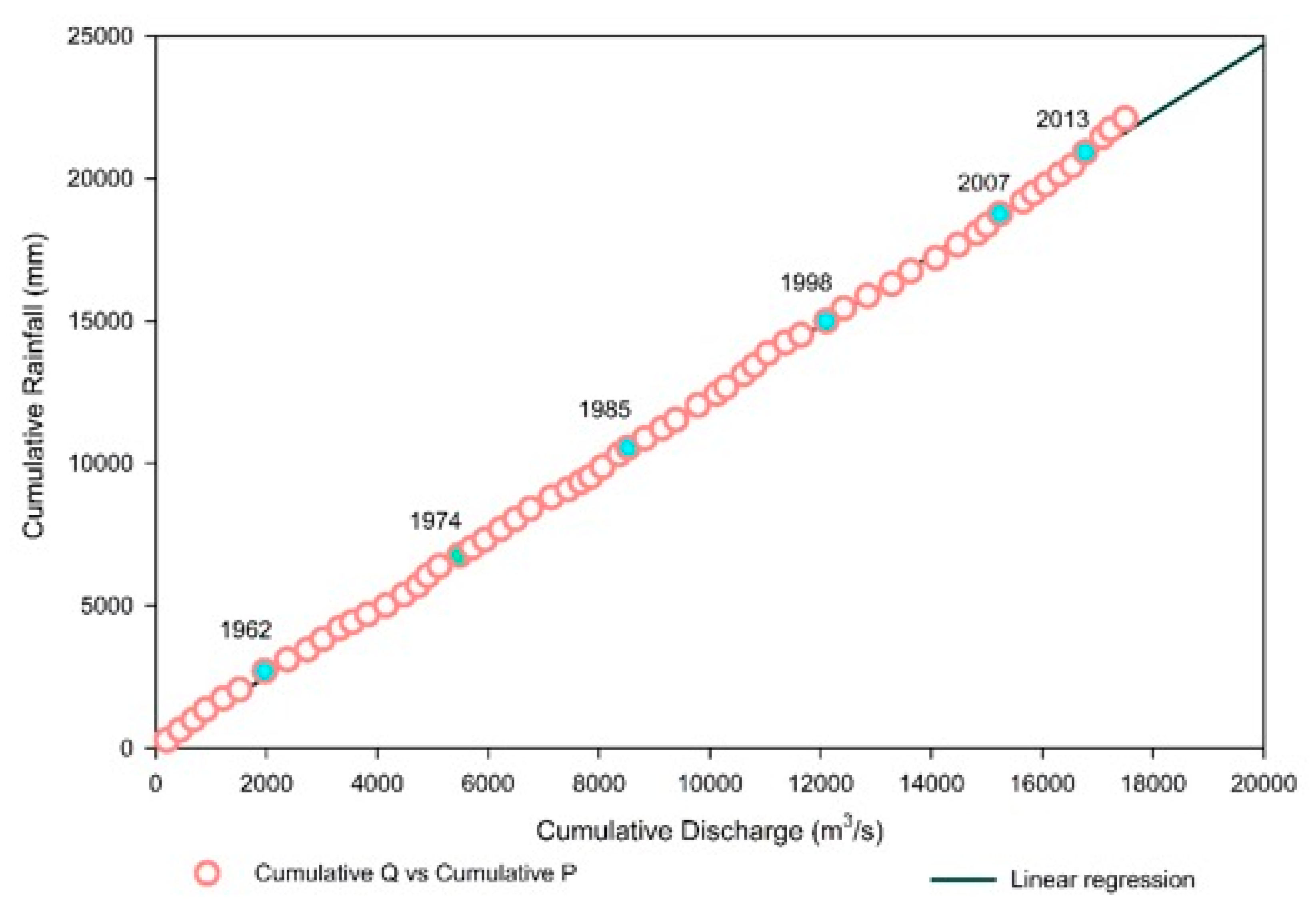
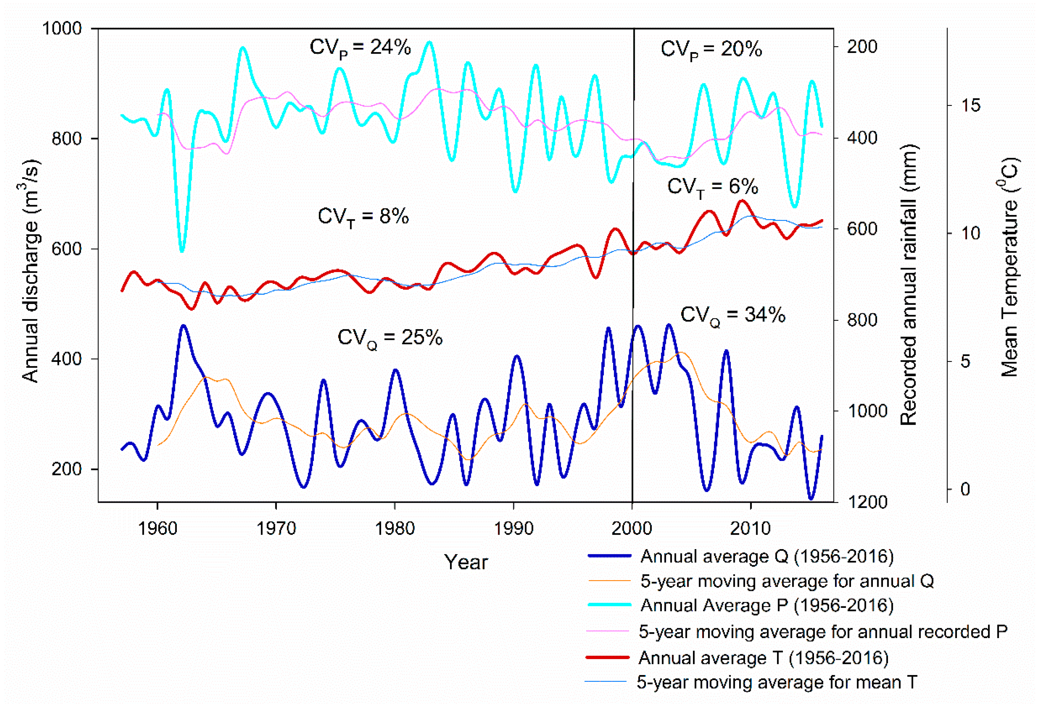
We saw that the escalated variation in hydro-meteorological parameters revealed by the previously discussed CV values was reaffirmed by the MK-S test for the time period of 2000–2016 compared to the years 1956–1999. The trend of rainfall pattern in the LRB during the two time spans was shown to have undergone a decrease in the latter time span that was also of greater magnitude, as exposed by Sen’s slope estimator. However, the decrease was not significant. Looking at the temperature change trend in the LRB during the two time spans, a significant increase in the temperature was revealed by the MK-S test, with a rapid rise in temperature in the study time span compared to the previous long-term time period. The authors of [81] also reported a significant increase in all the QTP basins including the LRB, with a range of 0.03–0.06 °C year−1, which was similar to the findings of our study. The LR discharge trend revealed a non-significant increase in the former long-term time span. Conversely, for the study time span, we saw a significant decrease in the LR discharge with a larger magnitude, as estimated by the Sen’s slope. We saw that the rainfall also decreased along the same time span, and the temperature was seen to have risen, which could have a serious impact on the LR discharge in the form of lower precipitation and aggravated evapotranspiration in the LRB. However, it can be seen that the decrease in the magnitude of LR discharge during 2000–2016 was far more, which clearly leads to the conclusion that in addition to the climatic phenomena, some other factors were causing the pronounced decrease in LR discharge during 2000–2016. During these years, major hydraulic interventions were witnessed in the LRB in the form of dam construction, including the Zhikong hydropower project (2006) and the Pangduo hydropower project (2013). These hydraulic structures impounded the water and caused the prominent decrease in LR discharge.
The MK-S test revealed a decreasing LR trend for all the seasonal flows, and the decrease reached significance in wet summer season and the dry winter season. Sen’s slope estimator revealed that the greatest reduction in the LR discharge was experienced in the wet summer season, followed by the dry winter season. The spring season was shown to experience the lowest reduction in discharge. This phenomena of the LR discharge trend could be explained by the fact that the wet summer season was the peak flow time in the LRB, where the major portion of LR discharge was generated (~90%) during these months. This water was stored in the reservoirs built on the LR for the succeeding dry wet season with a minimum rainfall and was responsible for the significantly decreased LR discharge during peak flow season. The higher variability and non-significant decrease in the LR discharge during spring season could be attributed to the snow and glacier melting, which is a completely-climate driven phenomena in the LRB. Thus, the variation of LR discharge during spring season is highly prone to the snowfall received during the winter season. In LRB, from April to May is a melting season when air temperature is, on average, above zero [81]. This snowmelt contributes to LR discharge and hence stabilizes the effect of rising temperature in the form of evapotranspiration and may be a reason for smaller decrease in LR discharge during spring season. Increasing air temperatures lead to less snow accumulation in the winter and an earlier peak runoff in the spring, as well as reduced flows in summer and autumn [82,83,84,85]. The change in the streamflow regime results in a substantial impact on regional water resources and seasonal water supplies [86]. For the dry winter LR discharge, a significant decrease with a greater magnitude and lower variability compared to the spring season could have been a possible manifestation of the increase rate of temperature. The MK-S test showed a significant and intensified increase in temperature of the LRB for the years 2000–2016. Similar behavior was reported in [25] for the LRB, where the increase rate of the minimum temperature was found to be higher in spring and winter than in summer, whereas the maximum temperature showed the opposite trend. This increased minimum temperature is causing an overall warming of the LRB and is showing its effects in the form of evapotranspiration with minimal rainfall to balance it, thus leading to a decreased LR discharge during the dry winter season. Additionally, the water demand in the LRB during the dry winter months is met by ground water abstraction and the reservoir-stored water during the wet summer season. This is again a factor that affects the LRB’s hydrological behavior in dry spells of a year.
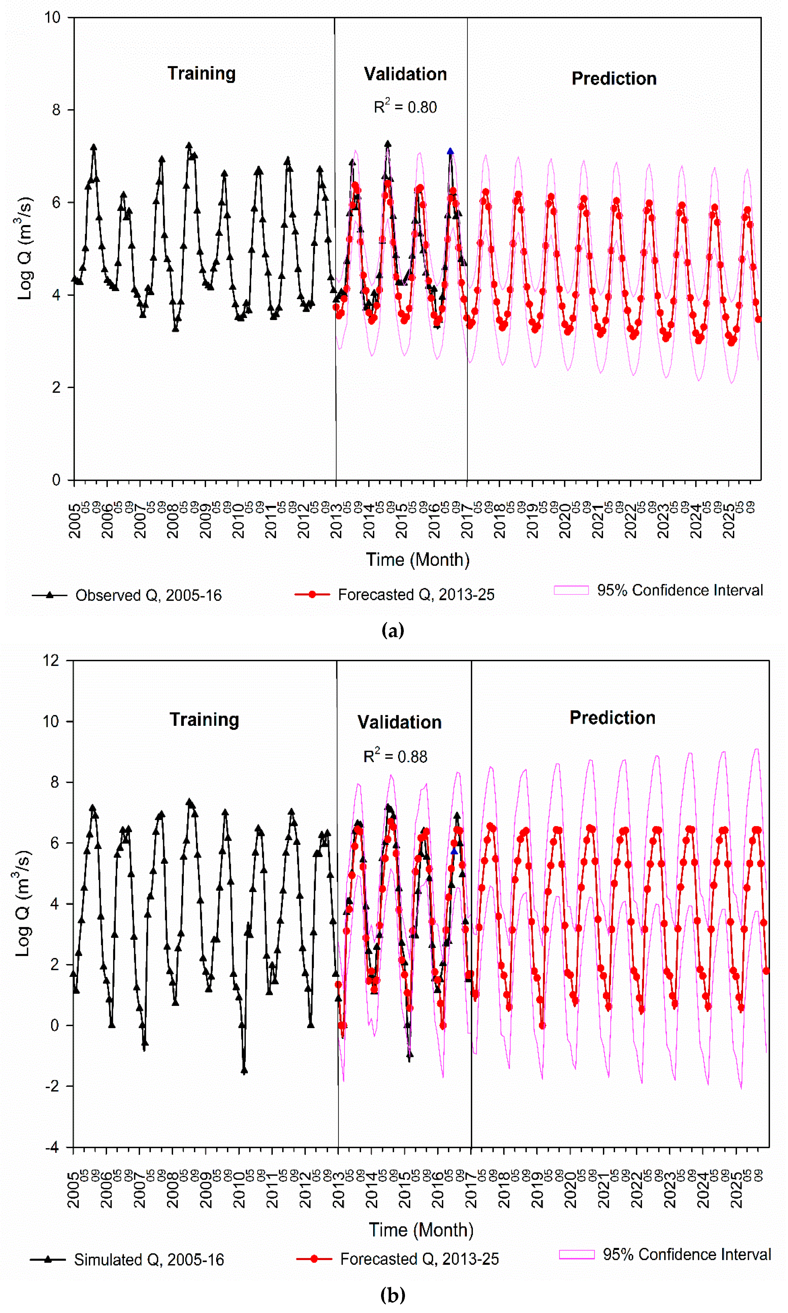
While predicting the LRB streamflow, we saw that in both situations, the LR discharge was predicted to decrease under the reservoir influence. This could be attributed to the inertial characteristic of the ARIMA model forecasts. If the historical data rise rapidly right before the peak value, they cannot be foreseen by the ARIMA model and the peak value would therefore be underestimated; however, if the rise is slow and steady, the rising trend would be expected to continue after the peak by the ARIMA model [28]. Here in the case of observed LR discharge, we saw a decreasing development through the years 2000–2016, which was confirmed by the MK-S test results presented earlier. Thus, ARIMA predicted an obvious decrease in the observation-based forecasted LR discharge. For the SWAT-simulation based LR discharge, the ARIMA model again predicted a decreasing yet stable future streamflow for 2017–2025, following the same behavior as the SWAT-simulated flow (Figure 7b).
The current study was intended to overcome the data scarcity issue of the study area, which is a major concern of the QTP catchments. In the current study, data availability on reservoir operations was a major constraint. Additionally, the data quality and availability for hydro-meteorological parameters included in the study were a prime concern for the trans-boundary Lhasa River.

5. Conclusions

The current study was carried out to evaluate the reservoir construction’s impact on LR discharge using double-mass curve analysis, estimating the CV for the closely related hydro-meteorological phenomena of LRB and identifying a trend on the hydro-meteorological behavior of the LRB using the well-known MK-S test. We found that:
  • The reservoir operation years showed themselves in the double-mass curve analysis for both the long-term (1956–2016) data series and the study time span of 2000–2016 as the break points in both curves.
  • CV values were individually calculated for two time spans of 1956–1999 and 2000–2016, and they showed that the variability in the hydro-meteorological phenomena for LRB was remarkably intensified in the latter time span compared to the years during the first time span. The variability in rainfall, temperature, and LR discharge escalated during the years 2000–2016. For the former time span, the LR discharge varied in accordance with the rainfall variation. For the latter time span, the variation in LR discharge was seen to be far greater than the rainfall variability. Additionally, the temperature change in the LRB was seen to be more rapid in the latter time period. However, the enormous variation in the LR discharge could not solely be attributed to the climatic factors, so some other factors are controlling the LR hydrological phenomena. This strong variation in LR discharge during the time span of 2000–2016 was the outcome of the two dams built over the LR. The Zhikong hydropower plant and the Pangduo power plant—which began operations in 2006 and 2013, respectively—have been influencing the LR discharge and causing a substantial variation in the LR discharge.
  • The MK-S test revealed a non-significant increase in the rainfall and a subsequent increase in LR discharge for the time 1956–1999. However, for the time span of 2000–2016, the rainfall in LRB experienced a non-significant decrease, whereas the LR discharge significantly decreased with an amplified magnitude that could be well-attributed to the reservoir functioning in the LRB. The temperature in the LRB was found to significantly decrease for the time spans of 1956–1999 and 2000–2016. The increase in temperature was more in the latter time span and potentially affected the snowmelt, evapotranspiration, and (ultimately) the discharge of the LR on a seasonal scale.
While predicting the LR discharge from 2017 to 2025, SWAT-ARIMA coupling revealed:
4.
The SWAT model was capable of simulating the LR discharge under reservoir influence, and simulation-based LR discharge can be a replacement to observed LR discharge. This could undisputedly aid in overcoming the hydrological data scarcity constraint in the LRB.
5.
The best-fitted seasonal ARIMA has forecasted a closely corresponding decreasing LR discharge time series for the years 2017–2025 when using the observation-based and simulation-based LR hydrological data. The observation-based predicted discharge was seen to decline at a greater extent, but the simulation-based predicted discharge was seen to follow the similar behavior to the observed LR discharge but while decreasing in the years from 2017 to 2025.
6.
This study revealed that a prominent climate change phenomena and human interferences are simultaneously affecting the hydrological regime of the LRB. This demands a more extensive study with a special influence on data availability for reservoir operations and procedures, water resource usage and allocation, ground water processes, etc. The study holds significance in assisting the water resource planning, management, availability, and requirement of water in hydropower generation, irrigation, domestic uses, etc., in the future for the LRB.

Author Contributions

This research is carried out in collaboration with all authors. Conceptualization, M.Y. and T.H.; methodology, M.Y.; software, M.Y. and S.A.H.; validation, M.Y. and S.A.H.; formal analysis, M.Y.; data curation, T.H.; writing—original draft preparation, M.Y.; writing—review and editing, T.H.; supervision, T.H.; project administration, T.H.; funding acquisition, T.H. All authors have read and agreed to the published version of the manuscript.

Funding

This study has been supported by the National Natural Science Foundation of China (Grant No. 91647204), and Wuhan Center of China Geological Survey (Grant No. 2020028; 2020023, YRSW-2020-359).

Acknowledgments

We thank three anonymous reviewers and editors for constructive suggestions and comments.

Conflicts of Interest

The authors declare no conflict of interest.

References

  1. Wang, Y.; Zhang, N.; Wang, D.; Wua, J.; Zhang, X. Investigating the impacts of cascade hydropower development on the natural flow regime in the Yangtze River, China. Sci. Total Environ. 2018, 624, 1187–1194. [Google Scholar] [CrossRef] [PubMed]
  2. Nilsson, C.; Reidy, C.A.; Dynesius, M.; Revenga, C. Fragmentation and Flow Regulation of the World’s Large River Systems. Science 2005, 308, 405. [Google Scholar] [CrossRef] [PubMed] [Green Version]
  3. Li, Q.; Yu, M.; Lu, G.; Cai, T.; Bai, X.; Xia, Z. Impacts of the Gezhouba and Three Gorges reservoirs on the sediment regime in the Yangtze River, China. J. Hydrol. 2011, 403, 224–233. [Google Scholar] [CrossRef]
  4. Guo, C.; Jin, Z.; Guo, L.; Lu, J.; Ren, S.; Zhou, Y. On the cumulative dam impact in the upper Changjiang River: Streamflow and sediment load changes. Catena 2020, 184, 104250. [Google Scholar] [CrossRef]
  5. Syvitski, J.P.M.; Vörösmarty, C.J.; Kettner, A.J.; Green, P. Impact of Humans on the Flux of Terrestrial Sediment to the Global Coastal Ocean. Science 2005, 308, 376. [Google Scholar] [CrossRef]
  6. Wang, H.; Bi, N.; Saito, Y.; Wang, Y.; Sun, W.; Zhang, J.; Yang, Z. Recent changes in sediment delivery by the Huanghe (Yellow River) to the sea: Causes and environmental implications in its estuary. J. Hydrol. 2010, 391, 302–313. [Google Scholar] [CrossRef]
  7. Dai, S.B.; Lu, X.X. Sediment load change in the Yangtze River (Changjiang): A review. Geomorphology 2014, 215, 60–73. [Google Scholar] [CrossRef]
  8. Dams and Development: A New Framework for Decision-Making: The Report of the World Commission on Dams; World Commission on Dams: Cape Town, South Africa, 2000.
  9. Zhao, Q.; Liu, S.; Deng, L.; Dong, S.; Yang, J.; Wang, C. The effects of dam construction and precipitation variability on hydrologic alteration in the Lancang River Basin of southwest China. Stoch. Environ. Res. Risk Assess. 2012, 26, 993–1011. [Google Scholar]
  10. Li, D.; Long, D.; Zhao, J.; Lu, H.; Hong, Y. Observed changes in flow regimes in the Mekong River basin. J. Hydrol. 2017, 551. [Google Scholar] [CrossRef]
  11. Zhang, Q.; Xiao, M.; Liu, C.L.; Singh, V.P. Reservoir-induced hydrological alterations and environmental flow variation in the East River, the Pearl River basin, China. Stoch. Environ. Res. Risk Assess. 2014, 28, 2119–2131. [Google Scholar] [CrossRef]
  12. Gao, B.; Yang, D.; Zhao, T.; Yang, H. Changes in the eco-flow metrics of the Upper Yangtze River from 1961 to 2008. J. Hydrol. 2012, 448–449, 30–38. [Google Scholar] [CrossRef]
  13. Yang, Z.; Yan, Y.; Liu, Q. Assessment of the flow regime alterations in the Lower Yellow River, China. Ecol. Inform. 2012, 10, 56–64. [Google Scholar] [CrossRef]
  14. Zhang, Q.; Zhang, Z.; Shi, P.; Singh, V.P.; Gu, X. Evaluation of ecological instream flow considering hydrological alterations in the Yellow River basin, China. Glob. Planet. Chang. 2018, 160. [Google Scholar] [CrossRef]
  15. Li, J.; Ma, L. Background Paper: Chinese Renewables Status Report; IAEA: Vienna, Austria, 2009. [Google Scholar]
  16. Tahir, A.A.; Hakeem, S.A.; Hu, T.; Hayat, H.; Yasir, M. Simulation of snowmelt-runoff under climate change scenarios in a data-scarce mountain environment. Int. J. Digit. Earth 2019, 12, 910–930. [Google Scholar] [CrossRef]
  17. Arnold, J.G.; Williams, J.R.; Maidment, D.R. Continuous-time water and sediment routing model for large basins. J. Hydraul. Eng. 1995, 121, 171–183. [Google Scholar] [CrossRef]
  18. Shen, Z.Y.; Chen, L.; Chen, T. Analysis of parameter uncertainty in hydrological and sediment modeling using GLUE method: A case study of SWAT model applied to Three Gorges Reservoir Region, China. Hydrol. Earth Syst. Sci. 2012, 16, 121–132. [Google Scholar] [CrossRef] [Green Version]
  19. Du, J.; Ru, H.; Zuo, T.; Li, Q.; Zheng, D.; Chen, A.; Xu, Y.; Xu, C.Y. Hydrological simulation by SWAT model with fixed and varied parameterization approaches under land use change. Water Resour. Manag. 2013, 27, 2823–2838. [Google Scholar] [CrossRef]
  20. Zhou, F.; Xu, Y.; Chen, Y.; Xu, C.Y.; Gao, Y.; Du, J. Hydrological response to urbanization at different spatio-temporal scales simulated by coupling of CLUE-S and the SWAT model in the Yangtze River Delta region. J. Hydrol. 2013, 485, 113–125. [Google Scholar] [CrossRef]
  21. Liechti, T.; Cohen, J.; Matos, P.; Boillat, J.L.; Schleiss, A.J. Influence of hydropower development on flow regime in the Zambezi River Basin for different scenarios of environmental flows. Water Resour. Manag. 2015, 29, 731–747. [Google Scholar] [CrossRef]
  22. Bieger, K.; Hörmann, G.; Fohrer, N. Simulation of streamflow and sediment with the soil and water assessment tool in a data scarce catchment in the three Gorges region, China. J. Environ. Qual. 2014, 43, 37–45. [Google Scholar] [CrossRef] [PubMed]
  23. Francesconi, W.; Srinivasan, R.; Pérez-Miñana, E.; Willcock, S.P.; Quintero, M. Using the soil and water assessment tool (swat) to model ecosystem services: A systematic review. J. Hydrol. 2016, 535, 625–636. [Google Scholar] [CrossRef]
  24. Peng, D.; Chen, J.; Fang, J. Simulation of Summer Hourly Stream Flow by Applying TOPMODEL and Two Routing Algorithms to the Sparsely Gauged Lhasa River Basin in China. Water 2015, 7, 4041–4053. [Google Scholar] [CrossRef] [Green Version]
  25. Tian, P.; Lu, H.; Feng, W.; Guan, Y.; Xue, Y. Large decrease in streamflow and sediment load of Qinghai–Tibetan Plateau driven by future climate change: A case study in Lhasa River Basin. Catena 2020, 187, 104340. [Google Scholar] [CrossRef]
  26. Yasir, M.; Hu, T.; Samreen, A.H. Simulating reservoir induced Lhasa streamflow variability using ArcSWAT. Water 2020, 12, 1370. [Google Scholar] [CrossRef]
  27. Wu, J.; Chen, X.; Yu, Z.; Yao, H.; Li, W.; Zhang, D. Assessing the impact of human regulations on hydrological drought development and recovery based on a ‘simulated-observed’ comparison of the SWAT model. J. Hydrol. 2019, 577, 123990. [Google Scholar] [CrossRef]
  28. Wang, W. Stochasticity, Nonlinearity and Forecasting of Streamflow Processes; IOS Press: Amsterdam, The Netherlands, 2006. [Google Scholar]
  29. Box, G.E.P.; Jenkins, G.M. Time Series Analysis: Forecasting and Control; Holden-Day: San Francisco, CA, USA, 1976. [Google Scholar]
  30. Wang, Z.Y.; Qiu, J.; Li, F.F. Hybrid Models Combining EMD/EEMD and ARIMA for Long-Term Streamflow Forecasting. Water 2018, 10, 853. [Google Scholar] [CrossRef] [Green Version]
  31. Adheikary, S.K.; Rahman, M.; Gupta, A.D. A stochastic modelling technique for predicting groundwater table fluctuations with time series analysis. Int. J. Appl. Sci. Eng. Res. 2012, 1, 238–249. [Google Scholar]
  32. Valipour, M.; Banihabib, M.E.; Behbahani, S.M.R. Comparison of the ARMA and ARIMA and the autoregressive artificial neural network models in forecasting the monthly inflow of Dez dam reservoir. J. Hydrol. 2013, 476, 433–441. [Google Scholar] [CrossRef]
  33. Ahlert, R.; Mehta, B. Stochastic analyses and transfer functions for flows of the upper Delaware River. Ecol. Model. 1981, 14, 59–78. [Google Scholar] [CrossRef]
  34. Yurekli, K.; Kurunc, A.; Ozturk, F. Application of linear stochastic models to monthly flow data of Kelkit Stream. Ecol. Model. 2005, 183, 67–75. [Google Scholar] [CrossRef]
  35. Modarres, R.; Ouarda, T. Modelling heteroscedasticty of streamflow time series. Hydrol. Sci. J. 2013, 58, 54–64. [Google Scholar] [CrossRef]
  36. Ahmad, S.; Khan, I.H.; Parida, B. Performance of stochastic approaches for forecasting river water quality. Water Res. 2001, 35, 4261–4266. [Google Scholar] [CrossRef]
  37. Kurunç, A.; Yürekli, K.; Çevik, O. Performance of two stochastic approaches for forecasting water quality and streamflow data from Yeşilιrmak River, Turkey. Environ. Model. Softw. 2005, 20, 1195–1200. [Google Scholar] [CrossRef]
  38. Tayyab, M.; Zhou, J.; Zeng, X.; Adnan, R. Discharge Forecasting By Applying Artificial Neural Networks at the Jinsha River Basin, China. Eur. Sci. J. 2016, 12, 108–127. [Google Scholar] [CrossRef] [Green Version]
  39. Wu, X.; Li, Z.; Gao, P.; Huang, C.; Hu, T. Response of the Downstream Braided Channel to Zhikong Reservoir on Lhasa River. Water 2018, 10, 1144. [Google Scholar] [CrossRef] [Green Version]
  40. Mu, X.M.; Zhang, X.Q.; Gao, P.; Wang, F. Theory of double mass curves and its applications in hydrology and meteorology. J. China Hydrol. 2010, 30, 47–51. [Google Scholar]
  41. Vörösmarty, C.J.; Green, P.; Salisbury, J.; Lammers, R.B. Global water resources: Vulnerability from climate change and population growth. Science 2000, 289, 284–288. [Google Scholar] [CrossRef] [Green Version]
  42. Poff, N.; Brown, L. Sustainable water management under future uncertainty with eco-engineering decision scaling. Nat. Clim. Chang. 2015. [Google Scholar] [CrossRef] [Green Version]
  43. Griffin, R.C. Water Resource Economics: The Analysis of Scarcity, Policies, and Projects; MIT Press: Cambridge, MA, USA, 2016. [Google Scholar]
  44. McCabe, G.J.; Wolock, D.M. A step increase in streamflow in the conterminous United States. Geophys. Res. Lett. 2002, 29. [Google Scholar] [CrossRef]
  45. Rosenzweig, C.; Neofotis, P. Detection and attribution of anthropogenic climate change impacts. Wiley Interdiscip. Rev. Clim. Chang. 2013, 4, 121–150. [Google Scholar] [CrossRef] [Green Version]
  46. McCuen, R.H. Modeling Hydrologic Change: Statistical Methods; CRC Press: Boca Raton, FL, USA, 2016. [Google Scholar]
  47. Varis, O.; Kajander, T.; Lemmelä, R. Climate and water: From climate models to water resources management and vice versa. Clim. Chang. 2004, 66, 321–344. [Google Scholar] [CrossRef]
  48. Ganguli, P.; Ganguly, A.R. Space-time trends in US meteorological droughts. J. Hydrol. 2016, 8, 235–259. [Google Scholar]
  49. Supratid, S.; Aribarg, T.; Supharatid, S. An integration of stationary wavelet transform and nonlinear autoregressive neural network with exogenous input for baseline and future forecasting of reservoir in flow. Water Resour. Manag. 2017, 4023–4043. [Google Scholar] [CrossRef]
  50. Zhang, Q.; Singh, V.P.; Li, K.; Li, J. Trend, periodicity and abrupt change in streamflow of the East River, the Pearl River basin. Hydrol. Process. 2014, 28, 305–314. [Google Scholar] [CrossRef]
  51. Lloyd, C.E.M.; Freer, J.E.; Collins, A.L.; Johnes, P.J.; Jones, J.I. Methods for detecting change in hydrochemical time series in response to targeted pollutant mitigation in river catchments. J. Hydrol. 2014, 514, 297–312. [Google Scholar] [CrossRef]
  52. Welch, B.L. The generalization of student’s problem when several different population variances are involved. Biometrika 1947, 34, 28–35. [Google Scholar] [CrossRef]
  53. Jackson, F.L.; Hannah, D.M.; Fryer, R.J.; Millar, C.P.; Malcolm, I.A. Development of spatial regression models for predicting summer river temperatures from landscape characteristics: Implications for land and fisheries management. Hydrol. Process. 2017, 31. [Google Scholar] [CrossRef] [Green Version]
  54. Kisi, O.; Ay, M. Comparison of Mann-Kendall and innovative trend method for water quality parameters of the Kizilirmak River, Turkey. J. Hydrol. 2014, 513, 362–375. [Google Scholar] [CrossRef]
  55. Pettitt, A.N. A non-parametric approach to the change-point problem. Appl. Stat. 1979, 28, 126–135. [Google Scholar] [CrossRef]
  56. Helsel, D.R.; Frans, L.M. Regional Kendall test for trend. Environ. Sci. Technol. 2006, 40, 13. [Google Scholar] [CrossRef]
  57. Libiseller, C. MULTMK/PARTMK. In A Program for Computation of Multivariate and Partial MANN-Kendall Test; LIU: Linköping, Sweden, 2004. [Google Scholar]
  58. Kliment, Z.; Matouskova, M. Runoff changes in the Šumava Mountains (Bohemian Forest) and the foothill regions: Extent of influence by human impact and climate changes. Water Resour. Manag. 2009, 23, 1813–1834. [Google Scholar] [CrossRef]
  59. Mann, H.B. Nonparametric test against trend. Econometrica 1945, 13, 245–259. [Google Scholar] [CrossRef]
  60. Kendall, M.G. Rank Correlation Methods; Charles Griffin: London, UK, 1975. [Google Scholar]
  61. Fu, G. Hydro-climatic trends of the Yellow River Basin for the last 50 years. Clim. Chang. 2004, 65, 149–178. [Google Scholar] [CrossRef] [Green Version]
  62. Zhang, D.; Chen, X.; Yao, H.; Lin, B. Improved calibration scheme of SWAT by separating wet and dry seasons. Ecol. Model. 2015, 301, 54–61. [Google Scholar] [CrossRef] [Green Version]
  63. Srinivasan, R.; Zhang, X.; Arnold, J.G. SWAT ungauged: Hydrological budget and crop yield predictions in the Upper Mississippi River Basin. Trans. ASABE 2010, 53, 1533–1546. [Google Scholar] [CrossRef]
  64. Nash, J.E.; Sutcliffe, J.V. River flow forecasting through conceptual models: Part 1. A discussion of principles. J. Hydrol. 1970, 10, 282–290. [Google Scholar] [CrossRef]
  65. Santhi, C.; Arnold, J.G.; Williams, J.R. Validation of the SWAT model on a large river basin with point and nonpoint sources. J. Am. Water Resour. Assoc. 2001, 37, 1169–1188. [Google Scholar] [CrossRef]
  66. Legates, D.R.; McCabe, G.J. Evaluating the use of “goodness-of-fit” measures in hydrologic and hydroclimatic model validation. Water Resour. Res. 1999, 35, 233–241. [Google Scholar] [CrossRef]
  67. De Winter, J.C.F.; Gosling, S.D.; Potter, J. Comparing the Pearson and Spearman correlation coefficients across distributions and sample sizes: A tutorial using simulations and empirical data. Psychol. Methods 2016, 21, 273–290. [Google Scholar] [CrossRef]
  68. Kendall, M.; Gibbons, J.D. Rank Correlation Methods. Charles Griffin Book Series, 5th ed.; Oxford University Press: Oxford, UK, 1990; ISBN 978-0195208375. [Google Scholar]
  69. Akaike, H. Information theory and an extension of the maximum likelihood principle. In 2nd International Symposium Information Theory; Petrov, B.N., Csak, F., Eds.; Akademia Kiado: Budapest, Hungary, 1973; pp. 267–281. [Google Scholar]
  70. Akaike, H. A new look at the statistical model identifiacation. IEEE Trans. Autom. Control. 1974, 19, 716–723. [Google Scholar] [CrossRef]
  71. McQuarine, A.D.R.; Tsai, C.L. Regression and Time Series Model Selection; World Scientific: Singapore, 1998. [Google Scholar]
  72. Yaya, O.; Fashae, A.O. Seasonal fractional integrated time series models for rainfall data in Nigeria. Theor. Appl. Climatol. 2014, 120, 99–108. [Google Scholar] [CrossRef]
  73. Ghimire, B. Application of ARIMA Model for River Discharges Analysis. J. Nepal Phys. Soc. 2017, 4, 27–32. [Google Scholar] [CrossRef] [Green Version]
  74. Ljung, G.M.; Box, G.E. On a measure of lack of fit in time series models. Biometrika 1978, 65, 297–303. [Google Scholar] [CrossRef]
  75. Searcy, J.K.; Hardison, C.H. Double-mass curves. In Manual of Hydrology: Part 1 General Surface-Water Techniques; Geological Survey Water-Supply Paper 1541–B; U.S. Department of Interior: Washington, DC, USA, 1960. [Google Scholar]
  76. Kliment, Z.; Matoušková, M.; Ledvinka, O.; Královec, V. Trend analysis of rainfall-runoff regimes in selected headwater areas of the Czech Republic. J. Hydrol. Hydromech. 2011, 59, 36–50. [Google Scholar] [CrossRef] [Green Version]
  77. Chen, J.; Finlayson, B.L.; Wei, T.; Sun, Q.; Webber, M.; Li, M.; Chen, Z. Changes in monthly flows in the Yangtze River, China-with special reference to the Three Gorges Dam. J. Hydrol. 2016, 536, 293–301. [Google Scholar] [CrossRef]
  78. Guo, L.; Su, N.; Zhu, C.; He, Q. How have the river discharges and sediment loads changed in the Changjiang river basin downstream of the three gorges dam? J. Hydrol. 2018, 560, 259–274. [Google Scholar] [CrossRef] [Green Version]
  79. Moriasi, D.; Arnold, J.; VanLiew, M.; Bingner, R.; Harmel, R.; Veith, T. Model evaluation guidelines for systematic quantification of accuracy in watershed simulations. ASABE 2007, 50, 885–900. [Google Scholar] [CrossRef]
  80. Searcy, J.K. Flow-Duration Curves, Manual of Hydrology: Part 2, Low-Flow Techniques; United States Geological Survey: Reston, VA, USA, 1959.
  81. Cuo, L.; Li, N.; Liu, Z.; Ding, J.; Liang, L.; Zhang, Y.; Gong, T. Warming and human activities induced changes in the Yarlung Tsangpo basin of the Tibetan plateau and their influences on streamflow. J. Hydrol. Reg. Stud. 2019, 25, 100625. [Google Scholar] [CrossRef]
  82. Mote, P.W.; Hamlet, A.F.; Clark, M.P.; Lettenmaier, D.P. Declining mountain snow pack in western North America. Bull. Am. Metab. Soc. 2005, 86, 39–49. [Google Scholar] [CrossRef]
  83. Cayan, D.R.; Kammerdiener, S.A.; Dettinger, M.D.; Caprio, J.M.; Peterson, D.H. Changes in the onset of Spring in the Western United States. Bull. Am. Metab Soc. 2001, 82, 399–415. [Google Scholar] [CrossRef] [Green Version]
  84. Stewart, I.; Cayan, D.C.; Dettinger, M.D. Changes in snowmelt runoff timing in Western North America under a ‘business as usual’ climate change scenario. Clim. Chang. 2004, 62, 217–232. [Google Scholar] [CrossRef]
  85. IPCC. Climate Change; Synthesis report; IPCC: Geneva, Switzerland, 2007. [Google Scholar]
  86. Li, L.; Xu, H.; Chen, X. Streamflow Forecast and Reservoir Operation Performance Assessment under Climate Change. Water Resour. Manag. 2010, 24, 83. [Google Scholar] [CrossRef]
Figure 1. Location map of the Lhasa River Basin extracted from the Advanced Thermal Emission and Reflection Radiometer, Global Digital Elevation Model (ASTER GDEM) dataset showing hydrological and meteorological stations, hydropower plants, and some other features of the study area.
Remotesensing 13 01382 g001
Figure 2. Schematic representation of reservoir impact evaluation, seasonal AutoRegressive Integrated Moving Average (SARIMA) and Soil and Water Assessment Tool (SWAT) model setup for the current study. LR: Lhasa River; DMC: double-mass curve; MK-S: non-parametric Mann–Kendall test; CV: coefficient of variability; PACF: partial autocorrelation function; AIC: Akaike’s information criterion; BIC: Bayesian information criterion; RMSE: root mean square error; MAPE: mean absolute percentage error; Q: Discharge (m3/s).
Remotesensing 13 01382 g002
Figure 3. Double-mass curve for cumulative rainfall and cumulative discharge of the Lhasa River for the time span of 1956–2016. The years for change in hydrological time series are highlighted and supported by text.
Remotesensing 13 01382 g003
Figure 4. Double-mass curve for the cumulative rainfall and cumulative discharge of the Lhasa River for the time span of 2000–2016. The years for change in hydrological time series are supported by the text.
Remotesensing 13 01382 g004
Figure 5. Changes of annual river discharge (at the Lhasa hydrometric station), annual mean temperature, and annual recorded precipitation for the Lhasa River Basin from 1956 to 1999 and from 2000 to 2016 (study time period with reservoirs functioning in the study area).
Remotesensing 13 01382 g005
Figure 6. (a) SWAT simulation of Lhasa River discharge recorded at the Lhasa hydrometric station for time span of 2005–2016. (b) Comparison of observed and SWAT-simulated Lhasa River discharge from 2005 to 2016.
Remotesensing 13 01382 g006
Figure 7. (a) Forecasted monthly Lhasa River streamflow for time span of 2013–2025 using the observed hydrological time series from 2005 to 2016. SARIMA model validation years from 2013 to 2016 are marked. (b) Forecasted monthly Lhasa River streamflow for time span of 2013–2025 using SWAT-simulated hydrological time series from 2005 to 2016. SARIMA model validation years from 2013 to 2016 are marked.
Remotesensing 13 01382 g007
Figure 8. (a) Comparison between observation-based and SWAT-simulation-based Lhasa River forecasted flow from 2017 to 2025. (b) Scatter plot of observation-based and simulation-based forecasted monthly Lhasa River discharge for 2017–2025.
Remotesensing 13 01382 g008
Figure 9. Flow–duration curves for the monthly observed, forecasted observation-based, and SWAT-simulation-based Lhasa River discharge.
Remotesensing 13 01382 g009
Table 1. Trend analysis on hydro-meteorological variables of the Lhasa River Basin. MK–τ represents Mann–Kendall’s trend at p = 0.05 (bold values are significant at p-value), and S represents the Sen’s slope estimator for change. The negative sign indicates a decrease.
Rainfall (P)Temperature (T)Discharge (Q)
1956–19992000–20161956–19992000–20161956–19992000–2016
MK–τ0.04−0.130.540.440.030.41
S0.52 (mm yr−1)−4.30 (mm yr−1)0.03 (°C yr−1)0.06 (°C yr−1)0.30 (m3 s−1 yr−1)−14.02 (m3 s−1 yr−1)
Table 2. The change and trend on seasonal Lhasa River discharge for the time period of 2000–2016. CV stands for coefficient of variation, MK–τ represents Mann–Kendall’s trend at p = 0.05 (bold values are significant at p), and S represents the Sen’s slope estimator for change in LR discharge (m3 s−1 month−1). The negative sign indicates a decrease.
Dry Winter Season (Nov-Feb)Spring Season (Mar-May)Wet summer Season (Jun-Oct)
CV47%56%62%
MK–τ0.28−0.140.27
S−0.6 (m3 s−1 yr−1)−0.4 (m3 s−1 yr−1)−5.6 (m3 s−1 yr−1)
Table 3. Sensitivity of selected parameters in influencing Lhasa River flow.
NoParameterParameter DescriptionMethod chosenRange Min-MaxFitted Valuet-statp-ValueRank
1.r__SOL_BDSoil bulk density (mg/m3)Relative−0.5–0.50.172.2870.0451
2.v__EPCOPlant uptake compensation factorReplace−1–10.651.8300.0972
3.v__GW_REVAPGround water “revap” coefficientReplace0.02–0.20.131.2490.2403
4.v__ESCOSoil evaporation compensation factorReplace0.01–10.85−0.7110.4924
5.v__GW_DELAYGround water delay (days)Replace0–50012.500.6300.5425
6.r__OV_NManning’s “n” value for overland flowRelative−0.5–0.5−0.020.3970.6996
7.r__SOL_AWCAvailable water capacity of soil layer (mm H2O/mm soil)Relative−0.2–0.20.07−0.2040.8427
8.r__SOL_KSaturated hydraulic conductivity (mm/h)Relative−0.5–0.50.470.1820.8588
9.r__CN2Initial SCS curve number for soil condition IIRelative−0.2–0.0−0.17−0.0220.9829
“r” denotes the relative method, and “v” denotes the replace method.
Table 4. Performance of the SWAT model in simulation of Lhasa River flow under reservoir operations. p-factor: percentage of data that is enclosed by the 95PPU band; r-factor: the average width of the 95PPU band divided by the standard deviation of the measured variable (from 0 to ∞, with 0 showing perfect match).
No.Performance Criteria2000–2016 (00–04 Warm-Up)
Calibration (05–10)Validation (11–16)
1.p-factor0.960.50
2.r-factor1.090.47
3.R20.910.58
4.NSE0.860.50
5.PBIAS5.55.5
Table 5. Statistical correlation of observed and SWAT-simulated Lhasa River discharge.
No.Correlation CoefficientValue
1.Pearson’s correlation0.87
2.Spearman’s correlation0.87
3.Kendall’s rank correlation0.68
Bold values are significant at p = 0.05.
Table 6. Performance of SARIMA model in predicting Lhasa River streamflow from 2017 to 2025 using observed and simulated hydrological time series.
Performance CriterionForecasted QobsForecasted Qsim
AIC76.7199.4
BIC91.28209.12
RMSE0.29 (m3/s)0.65 (m3/s)
MAPE4.02%31.09%
Table 7. Statistical correlation between forecasted observation-based and simulation-based Lhasa River discharge, 2017–2025.
No.Correlation CoefficientValue
1.Pearson’s correlation0.95
2.Spearman’s correlation0.95
3.Kendall’s rank correlation0.80
Bold values are significant at p = 0.05.
Publisher’s Note: MDPI stays neutral with regard to jurisdictional claims in published maps and institutional affiliations.

