GPR-Based Automatic Identification of Root Zones of Influence Using HDBSCAN

Abstract

The belowground root zone of influence (ZOI) is fundamental to the study of the root–root and root–soil interaction mechanisms of plants and is vital for understanding changes in plant community compositions and ecosystem processes. However, traditional root research methods have a limited capacity to measure the actual ZOIs within plant communities without destroying them in the process. This study has developed a new approach to determining the ZOIs within natural plant communities. First, ground-penetrating radar (GPR), a non-invasive near-surface geophysical tool, was used to obtain a dataset of the actual spatial distribution of the coarse root system in a shrub quadrat. Second, the root dataset was automatically clustered and analyzed using the hierarchical density-based spatial clustering of applications with noise (HDBSCAN) algorithm to determine the ZOIs of different plants. Finally, the shape, size, and other characteristics of each ZOI were extracted based on the clustering results. The proposed method was validated using GPR-obtained root data collected in two field shrub plots and one simulation on a dataset from existing literature. The results show that the shrubs within the studied community exhibited either segregated and aggregated ZOIs, and the two types of ZOIs were distinctly in terms of shape and size, demonstrating the complexity of root growth in response to changes in the surrounding environment. The ZOIs extracted based on GPR survey data were highly consistent with the actual growth pattern of shrub roots and can thus be used to reveal the spatial competition strategies of plant roots responding to changes in the soil environment and the influence of neighboring plants.

1. Introduction

Root systems are essential parts of plants, as they absorb water and nutrients and support the aboveground plant structure [1,2]. Because roots are flexible, their growth is influenced by the soil environment and the root systems of surrounding plants [3,4]. Root–root and root–soil interactions include competition for belowground space and nutrient resources, complementary utilization of resources, and competition for the sharing of growth space. Together, these interactions shape the morphological structures and spatial distributions of plant roots, so they are key factors in understanding changes in plant community and ecosystem processes. To further explore these interactions, the underground root zone of influence (ZOI) of an individual plant needs to be accurately identified. Because the ZOI represents the maximum soil space occupied by the root system of an individual plant, its size and shape determine the plant’s ability to access soil resources effectively and compete within the ecosystem [5]. Furthermore, the ZOI can be applied for predicting and modeling plant root interactions and therefore aid in exploring the mechanisms by which plants achieve efficient resource use and competition [6].

The concept of the ZOI was introduced in previous studies that examined plant competition for belowground resources, and it has mainly been used to predict root distributions under the influence of competition [7,8]. There are three common methods for studying ZOI: theoretical modeling, the tracer method, and the excavation method. Theoretical modeling defined the ZOI according to the set parameters and conditions and simulated the space occupied by plant roots under the conditions with or without competition [9,10,11]. The compensatory growth of roots [12] or the idea of evolutionary game theory [13] was introduced to model the underground competitive pressure of plant roots and its influence on the size and shape of the ZOI. However, these studies are speculations from theoretical models and lack field validations. As for the tracer method, nutritional tracers were used to obtain the distribution of lateral roots and then quantify the shape and size of ZOI under controlled experiments in the field [6,14,15]. The ZOI derived by this method showed that the extent of lateral roots was much more extensive than previously recognized, both horizontally and vertically, and the shape of the ZOI was irregular, instead of being a plant-centered circular shape [6]. However, the tracer method needs to be carried out under controlled experimental conditions and is time consuming, which limited its measurement area and cannot adequately explain the interaction mechanisms among roots within a plant community. In addition, the traditional excavation method has been used to expose and describe the morphology of a root system and further determine the ZOI [16]. However, this approach is also laborious and destructive. The disturbance to the root zone introduced during excavation prevents ongoing investigations of the interactions among plants in a community. Therefore, the in-depth understanding of the ZOI and root interaction requires an effective, non-destructive, and automatic method to support the field research and verification of its theoretical models.

Ground-penetrating radar (GPR), a non-invasive geophysical technique, has been successfully applied in observational and quantitative studies of plant coarse roots in recent years [17,18,19]. GPR generates electromagnetic waves of specific frequencies that pass through the interfaces between subsurface media with different dielectric permittivities, and a receiving antenna gathers energy reflected by the target. The attributes and locations of belowground targets can be determined by analyzing the travel times, amplitudes, and shapes of the reflected waves [18]. In general, the water content of a root is higher than that of the surrounding soil, and this difference produces a sufficient permittivity gradient for GPR to detect and identify roots [20]. Compared with traditional methods in root research, GPR has several advantages: (1) it permits long-term, non-destructive, repeated observations of target roots; (2) it can accurately identify and localize coarse roots; and (3) root detection can be achieved rapidly at relatively large spatial scales. Therefore, GPR provides an opportunity to obtain more complete information on the distribution and structure of plant roots at landscape scales.

Recently, GPR has been widely used in studying coarse roots, including in studies on root parameter estimation (i.e., root biomass and diameter), root spatial distribution detection, and root morphological structure reconstruction [19,21,22]. Wu et al. [21] used root points to analyze the spatial distribution patterns of belowground roots and then reconstructed the three-dimensional morphological structure of the roots. Cui et al. [22] used a dual-frequency GPR with two antenna frequencies (400 and 900 MHz) to map the three-dimensional distribution of roots in semiarid shrublands in China and analyze the influence of interplant root competition on root distributions. Generally, the point clouds generated by GPR surveys correspond to the spatial discretization of the root system, which is highly consistent with the actual spatial distributions of plant roots in the field. However, that study focused on the overall spatial distribution of all the root points detected by GPR, and it did not try to relate those root systems to specific plants or identify each plant’s ZOI [20].

Given that root density generally follows a bell shape, the root point density should be the highest beneath the canopy center. Therefore, based on the distribution of roots mapped by GPR, it is possible to group root points to each plant automatically using a clustering algorithm based on distances between points. Among the existing clustering methods, the hierarchical density-based spatial clustering of applicants with noise (HDBSCAN) algorithm provides a competitive choice, which clusters points according to their distribution densities [23,24]. The HDBSCAN algorithm has been applied in a wide range of research fields, such as environment, urban road, and medical studies. For example, Veerhoek [25] used HDBSCAN to identify eutrophication zones in the offshore and coastal areas. Rosalina et al. [26] used HDBSCAN in the road network data to group roads at different resolutions. Lin et al. [27] successfully identified the outliers after clustering and verified the clinical results of stroke. Therefore, it is meaningful to explore the feasibility of HDBSCAN to cluster root points and map the ZOIs of individual plants.

Caragana microphylla is a dominant species in the process of shrub encroachment in the grasslands of Inner Mongolia, China, and the spatial distribution of its root system largely determines the system patterns and the carbon and water cycles as well as the development process of the shrub in scrub ecosystems [28]. Therefore, the identification and analysis of the ZOIs in a C. microphylla community could help understand the interactions among root systems within scrub communities in semiarid environments.

This study aimed to provide a novel technical method to identify the ZOIs of individual plants under field conditions through GPR root detection. The GPR surveys were conducted in the semiarid grassland in Inner Mongolia, China, to nondestructively obtain the spatial distribution of root points within a community of C. microphylla. The ZOI of each shrub was automatically identified through spatial density clustering of the detected root points using the HDBSCAN algorithm. The proposed approach has the potential for the large-scale mapping of plant ZOIs, which will help analyze the size, shape, and other characteristics of ZOI. This will offer new insights into the complex interactions between root systems of different plants.

2. Materials and Methods

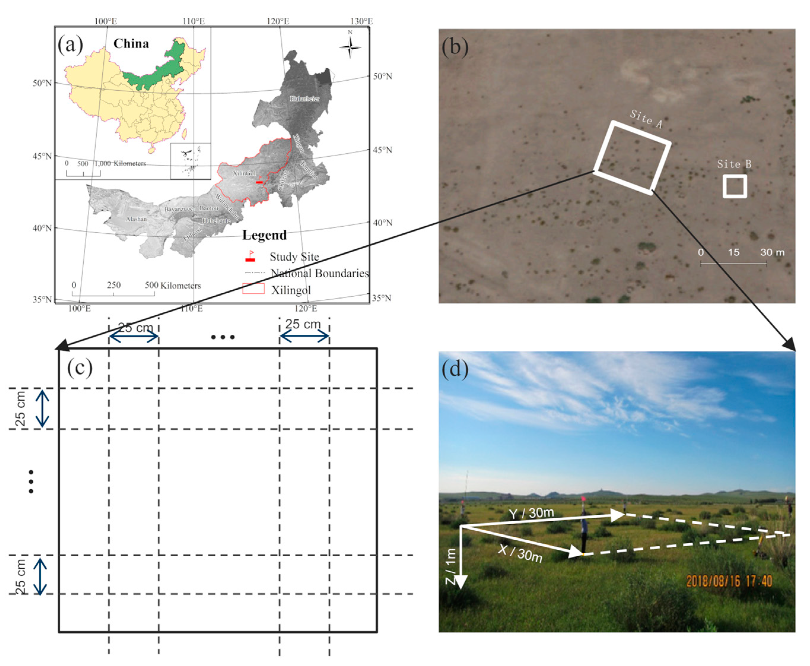
2.1. Study Site

Our study sites were located in the Xilin Gol grassland (43°54′58″ N, 116°12′16″ E) in Inner Mongolia (Figure 1a), a typical semiarid area in northern China, with an average altitude of 988.5 m. This region has a temperate continental climate with an average annual temperature of 2.6 °C and an average annual rainfall of approximately 350 mm (mostly occurring in July to September) [29]. C. microphylla is the dominant species in this area. Its root system is mainly distributed in the soil at a depth of 0–100 cm, where it accounts for more than 92% of the total root biomass, and its maximum vertical root system depth is about 2.2 m. Its lateral roots are particularly developed, which, when combined with the sandy soil it grows in, makes it an excellent target for GPR detection [30,31].

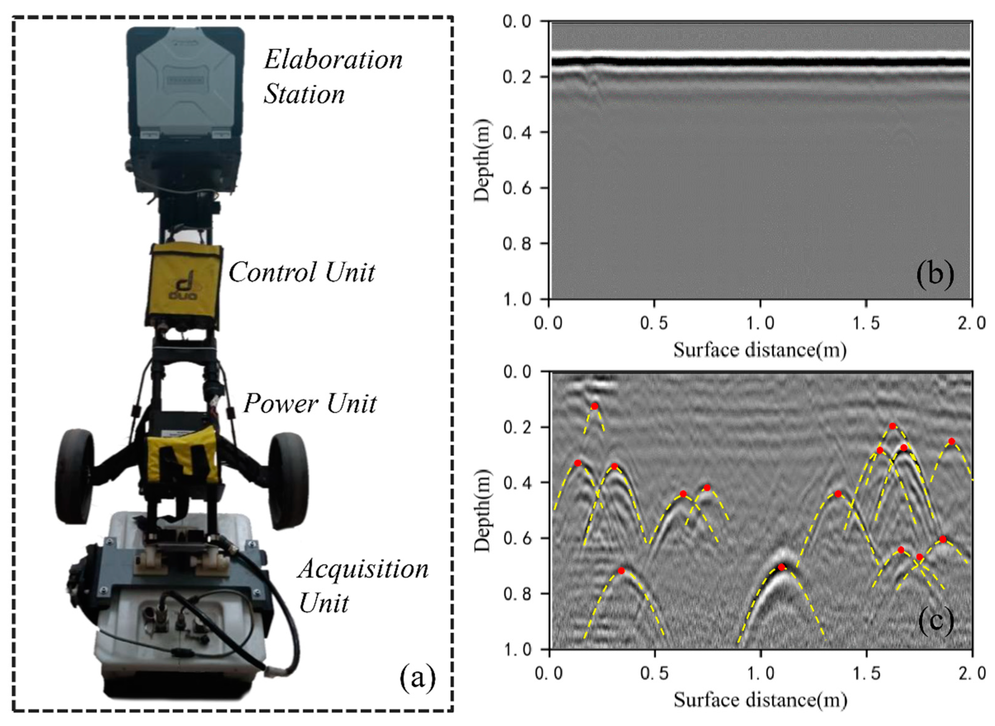
2.2. Field Data Collection

The GPR data were collected in August 2018. Site A was the primary data collection zone (30 m × 30 m) within the experimental study area (Figure 1b). We collected both aboveground biological parameters and belowground root points at Site A. The survey processes included: (1) acquiring position by Global Position System (GPS); (2) measuring the height, crown width, and relative position coordinates of each shrub (Figure 2); (3) setting up a survey network with survey lines at 25 cm intervals, totaling 242 lines (Figure 1c); (4) assembling the dual-frequency (400 and 900 MHz) GPR system (RIS MF Hi-Mod; Ingegneria Dei Sistemi Inc., Italy) by equipping the transmitting antenna and receiving antenna at the bottom of a small cart (Figure 3a) which is close to the ground surface; and (5) pushing the cart along the survey line to collect the raw GPR data. Detailed information of root GPR data collection is also provided in [32]. Root points at this site were determined through postprocessing and interpretation of these GPR images.

2.3. GPR Data Processing

We preprocessed the raw GPR images before extracting root information to eliminate noise and enhance the signal-to-noise ratio [33,34]. A GPR processing software, Reflex-Win 6.1 (Sandmeier Scientific Software, Germany), was used to process the raw GPR images (Figure 3b), including first arrival time pick-up, background removal, bandpass wave filtering, and amplitude gain. First arrival time pick-up was used to correct the vertical and horizontal scales on the GPR images. According to the energy difference before and after the first arrival time point, the maximum ratio of the summed energy of the two moving time windows is applied to each trace to detect the first arrival time [35]. During the GPR detection, there are many background noises, including noises caused by high and low frequencies [36]. The high-pass filtering was used to suppress background low-frequency noise, and bandpass filtering was used to eliminate the high-frequency noise. To compensate for the energy loss caused by scattering, dissipation, and medium attenuation, time-varying gain adjustments were applied on GPR images to strengthen root reflections [37]. During the GPR detection, there are many background noises, including horizontal bands caused by antenna–ground interaction, multiple reflections caused by signal reflections between subsurface layers, and high-frequency pulse. More details of the postprocessing of GPR images can be found in Guo et al. [32]. The processed signals of the coarse root reflections in the radar profiles had a typical hyperbolic shape (Figure 3c). The randomized Hough transform algorithm was used to automatically identify the hyperbolic characteristics of the root reflection signal and determine the locations of coarse roots according to the vertices of each hyperbola [38], thus obtaining a 3-D point cloud dataset of the coarse roots.

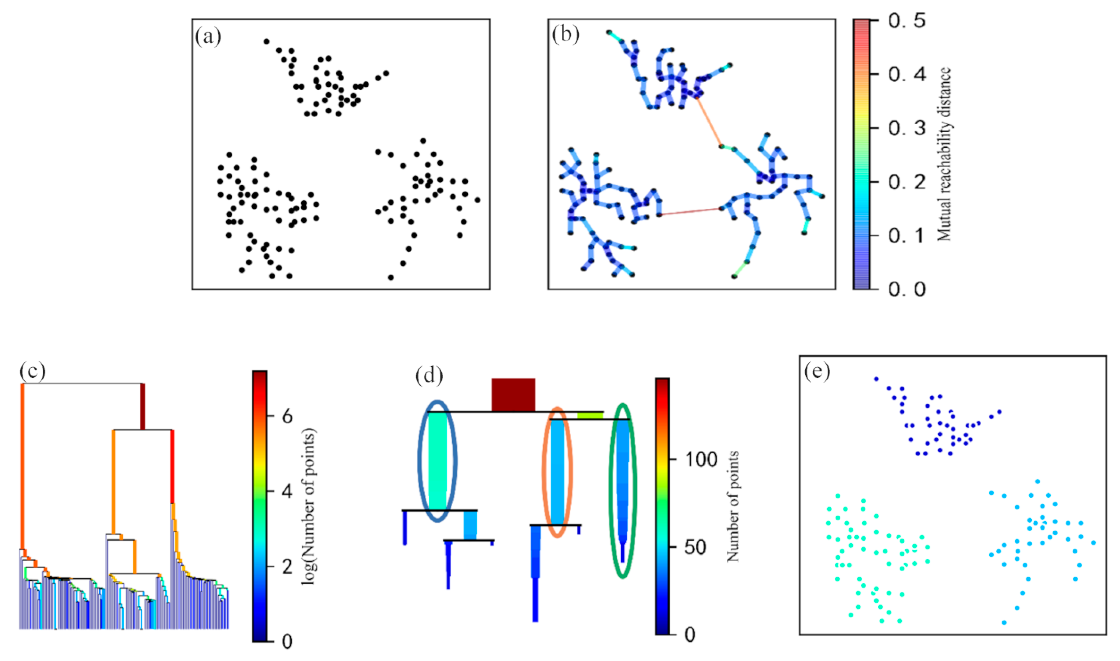
2.4. Identification of the ZOI from GPR-Based Root Measurements

A spatial density clustering method, the hierarchical density-based spatial clustering of applications with noise (HDBSCAN) algorithm, was used to analyze the distribution of root points identified by GPR and determine the ZOIs [23,39]. The HDBSCAN algorithm is a hierarchical clustering method based on non-parametric density estimations. It identifies clusters by combining the hierarchical structure and the mutual reachability distance to distinguish high-density regions separated by low-density regions [24]. HDBSCAN has several advantages over other algorithms: (1) by separating cluster and noise points, it extracts clusters effectively even when the data sample density is nonuniform; (2) its hierarchical clustering strategy helps interpret the structural relationships in complex datasets; (3) it requires the tuning of only a few insensitive parameters; and (4) its clustering stability index can be used to provide a reference for the final clustering result.

Many factors influence the number of root points and the ZOI of a plant (e.g., plant age, growth, and belowground microenvironment). The root densities surveyed by GPR reflect this variation, and the distribution density of roots determines the complexity of the belowground root distribution in a shrub population. The advantages of HDBSCAN can help it extract clustering results at different density levels through the hierarchical structure analysis of GPR-generated root points, which are then used to determine the ZOIs of different plants.

The HDBSCAN algorithm estimates the density of root points using the core distance, defined as the distance from a point $x$ to its k^th nearest neighbor point, $cor{e}_k\left(x\right)$. To separate a low-density area from a high-density area, the mutual reachability distance (MRD) is defined as:

$$d_{mreach-k}\left(x_a,x_b\right)=\max \left\{cor{e}_k\left(x_a\right),cor{e}_k\left(x_b\right),d\left(x_a,x_b\right)\right\}, x_a,x_b\in X$$

(1)

where $d_{mreach-k}\left(x_a,x_b\right)$ is the mutual reachability distance from point $x_a$ to point $x_b$, $cor{e}_k\left(x_a\right)$ is the core distance of $x_a$, $cor{e}_k\left(x_b\right)$ is the core distance of $x_b$, and $d\left(x_a,x_b\right)$ is the Euclidean distance from $x_a$ and $x_b$. The MRD is developed based on the core distance to enlarge the gap between a high-density region and a low-density region; thus, clusters using the MRD as a measurement tend to be identified in the high-density region. The MRD depends upon the choice of k, which is a classical smoothing factor in density estimations and can also be interpreted as a measure of how conservative clusters are [40]. Larger k values enlarge the core distance and the MRD. Thus, more points are discarded. In this study, discarded points were considered noise points.

The algorithm built a minimum spanning tree based on the mutual reachability distance matrix in which the vertices of the tree were the root points identified by GPR. The vertices were connected by edges, and the weight of each edge was the MRD between the connected root points (Figure 4a). The minimum spanning tree was built by connecting all root points with the smallest MRD sums (Figure 4b). Therefore, the edges could be sorted and merged in increasing order according to their corresponding MRDs in the minimum spanning tree. This allowed for the acquisition of a hierarchical cluster tree of density-based MRD values (Figure 4c). Then, the original tree was condensed by the minimum cluster size (m) to retain the root points belonging to clusters (potential ZOIs), and other points were discarded as noise. We assumed that the number of root points was related to plant size, so the parameter m depended on the minimum plant size. This parameter was used to denote the minimum number of root points in each ZOI, preventing clustering results that were too small and suppressing non-root point information. Finally, the stability index, $S_{cluster}$, was used to evaluate the clustering results [24]:

$$S_{cluster}={\sum }_{p\in cluster}^{}({\lambda }_p-{\lambda }_{birth})$$

(2)

where ${\lambda }_p$ represents the reciprocal of the corresponding edge weight (i.e., the MRD) when the root point $p$ in the clustering result is separated from this cluster, and ${\lambda }_{birth}$ represents the reciprocal of the corresponding edge weight when the new cluster is split. $S_{cluster}$ was employed to judge whether to merge subclasses of the same level (equal MRDs) into one cluster to form a ZOI in this study. If the stability of the sum of the two subclasses was less than previous levels, the two subclasses were merged (Figure 4d). The final clustering result consisted of multiple dense regions of root points extracted from the point clouds generated by GPR. These regions were considered ZOIs (Figure 4e).

2.5. Validation Method

2.5.1. Validation with Field Data

Due to the destruction of the soil environment and the difficulty of excavating large areas, it was unrealistic to dig up the entire root system to validate the ZOI results generated by the HDBSCAN clustering algorithm at Site A. Therefore, Site B as a smaller site (6 m × 6 m) reference was established for the validation of the clustering results. The aboveground parameters and root system were surveyed in the same way as at Site A. Then, each shrub’s roots were carefully excavated and exposed at Site B, layer by layer, trying to keep the root system intact to a depth of 1 m, and photos were taken to record the results. Since field GPR survey data and the clustering results are in 3-D, these results were projected to 2-D to compare the horizontal root distribution with the excavation results.

2.5.2. Validation with Simulated Data

In addition, a spatial distribution map of the root system obtained in a previous study was utilized to validate the accuracy and robustness of the ZOIs produced by the HDBSCAN algorithm [16]. The reference data consisted of a shrub root distribution map in a grid (10 m × 7 m) derived from a manual excavation and recording in the field (Figure 5a); the map shows detailed morphology and the distribution range of the root system of each plant. There were 50 plants in this area, with a variety of shrub types. A GPR survey was simulated by all root point positions based on the original book data (Figure 5a).

Based on Figure 5a, the locations of the coarse root determined by GPR are simulated according to the following criteria: (1) the original image (Figure 5a) was converted into vector root data through digital vectorization, and the vector root data were simplified by retaining the main branches and removing the small end branches, which might be challenging to distinguish in GPR field surveys; (2) the same survey gird and interval (Figure 1c) as prepared at Site A were used to set up the simulated survey line girds, and the reference root systems were assumed to be scanned by GPR following these survey lines; (3) the intersection points of root branches and simulated survey lines (i.e., the color dots in Figure 1b) were extracted to represent the discrete root points identified by GPR, producing the 2-D simulated root points data; and (4) the distance resolution of the survey wheel of the selected GPR system was used to delete the root points that were too close to each other. These processes were designed to make the simulated root points as consistent as possible with the root points measured by GPR in the field. A detailed description of simulating GPR-derived root points from the root distribution map can be found in Wu et al. [21].

Figure 5b was taken as the actual ZOI situation. The situations under different survey line intervals and angles were simulated, including survey line intervals of 10, 15, 20, and 25 cm, as well as survey lines with 10 cm intervals that were rotated counterclockwise by 30°, 45°, and 60°. This helped analyze the influence of changes in the survey line interval and direction on the clustering results. With both field-based and simulated datasets, the applicability of HDBSCAN on the identification of ZOIs was evaluated by comparing its clustering results with the reference.

2.6. Analysis of the Characteristics of ZOI

The Nightingale’s rose diagrams were used to preliminarily quantify the degree of asymmetry in each ZOI in eight directions to compare the differences of ZOIs. In this process, three parameters of each ZOI (i.e., the number of root points, the root extension distance, and the root depth) were normalized and expressed as three layers from the inside to the outside along each of the eight directions. The normalization formula was:

$$P_{i,j}=P_{i,j}/P_{i,max}$$

(3)

where $P_{i,j}$ is the value of the $i_{th}$layer in the$j_{th}$ direction, and $P_{i,max}$ is the max value of $P_{i,j}$ (j = 1, 2,…,8). We used a Python package, pyecharts, to produce ZOI rose diagrams. Based on the rose diagram data, the variance of the three parameters, representing the degree of the asymmetry in ZOI distribution, was calculated for each ZOI in each direction:

$$S_i^2=\frac{{\sum }_{j=1}^{j=8}{\left(P_{i,j}-{\overline{P}}_i\right)}^2}{8}$$

(4)

where $S_i^2$ and ${\overline{P}}_i$ are the variance and mean of the $i_{th}$layer, respectively. The projected area of each ZOI was calculated to illustrate the difference in size between the ZOIs. Then, grouping statistics were performed according to the characteristics of each ZOI.

3. Results

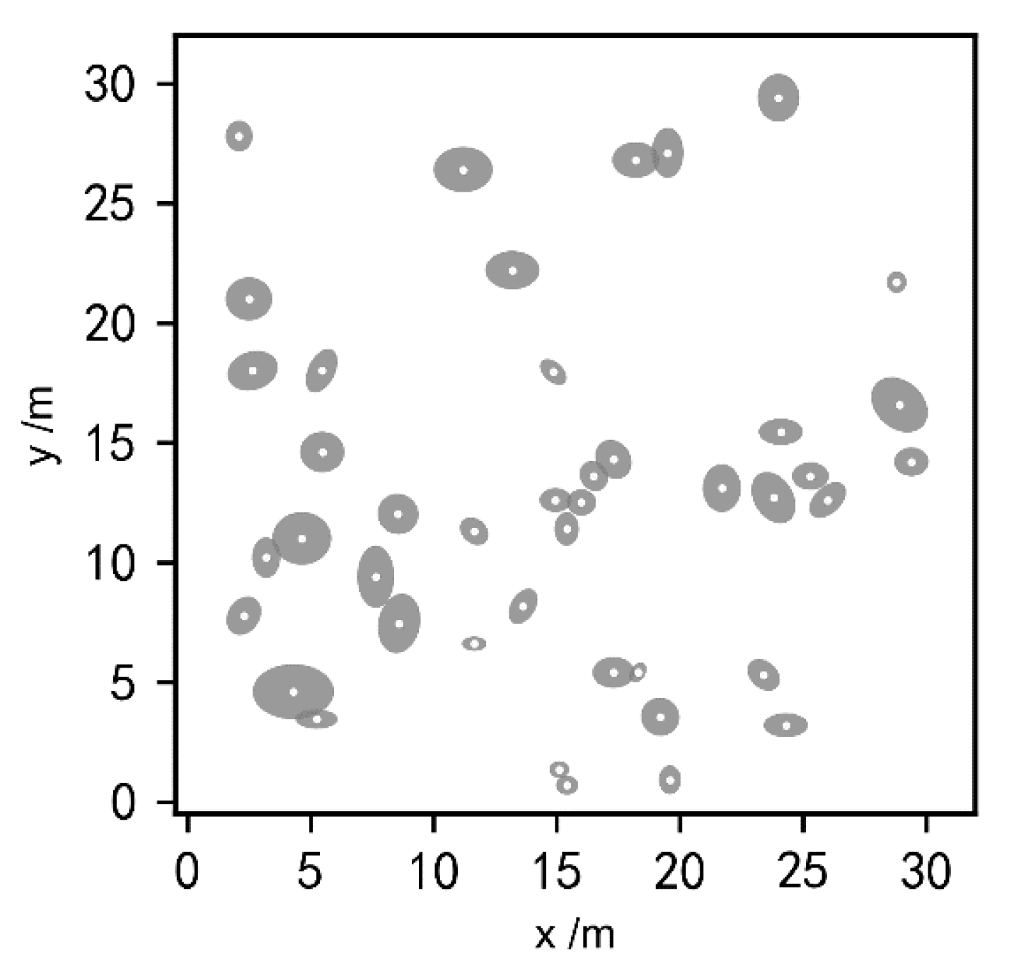
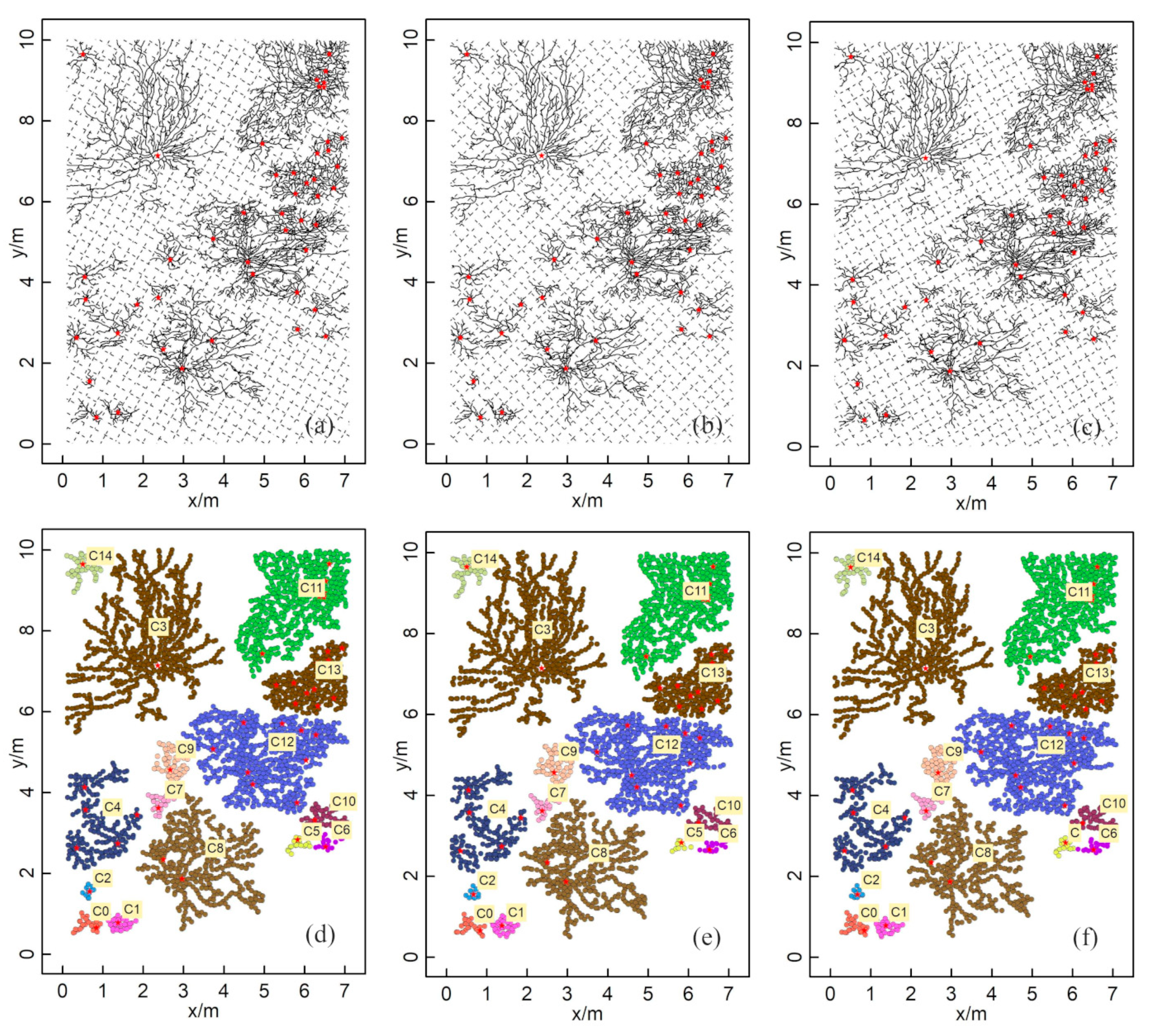
3.1. The Extraction of ZOIs Based on Field Data

The GPR survey and clustering results for Site A are shown in Figure 6. The number of root points interpreted from the GPR images was 6596 (Figure 6a), and the depths of the root points ranged from 0.1 to 1.3 m. Figure 6a reveals that the distribution of roots in all directions around each plant was uneven. Root point density varied with the distance between plants: the root points close to multiple plants were denser than those near a single plant. The parameters for the spatial density clustering analysis were tuned for this dataset (i.e., k = 3 and m = 13).

Some root systems of different plants were effectively isolated, indicating that the belowground ZOIs matched the distribution pattern of aboveground plants (e.g., C11). According to the clustering results, a total of 26 ZOIs were identified (Figure 6b), but this was fewer than the number of shrubs observed aboveground (43 shrubs). In such cases, some roots of multiple plants were indistinguishable and were grouped into the same ZOI (e.g., C14). That is, not every shrub’s ZOI was isolated from its neighbors, and some roots were separated (i.e., an individual plant with an independent ZOI), while others tended to be aggregated (i.e., multiple plants share the same ZOI).

The average crown size of the aboveground shrubs at this site was 1.75 m², and the ground projection was circular or elliptical; thus, the total projected area of crown size was 80.61 m², suggesting that the canopy-covered area made up to 8.96% of the total area. In comparison, the average size of a ZOI was 14.51 m², and the projected shape was irregular. The total projected ZOI area was 420.67 m², reaching 46.74% of the total area, so the roots extended far beyond the aboveground canopy.

The results of the survey and excavation at Site B are shown in Figure 7. Site B contained four shrubs, namely, T1, T2, T3, and T4, and their crown sizes were 3.70, 1.47, 0.11, and 1.95 m² (Figure 7a), respectively. The number of root points interpreted by the GPR survey was 591, with depths ranging from 0.1 to 1.3 m (Figure 7b). The root point distribution at Site B showed similar characteristics to that of Site A. Only two clusters were generated by the HDBSCAN cluster analysis: T1 and T2 were clustered together, while T3 and T4 were placed into one group, and many roots of different plants could not be separated (Figure 7b). According to the on-site excavation, the belowground roots of T1 and T2 were found to be intertwined and could not be completely separated, and the root distributions of T3 and T4 showed a similar pattern (Figure 7c). The excavation results indicate that the roots overlapping is a natural phenomenon in the C. microphylla population, which means that roots of different plants could share the same ZOI. The patterns uncovered at Site B also supported the rationality of multiple plants corresponding to the same ZOI that was also observed at Site A.

3.2. The Validation of ZOIs Based on the Simulated Data

The numbers of GPR-detected root points in the simulation data at 10, 15, 20, and 25 cm survey line intervals were 3217, 2198, 1592, and 1311, respectively (Figure 8a–d). The numbers of root points after clustering using the HDBSCAN algorithm were 3185, 2042, 1548, and 1266, and the corresponding numbers of clusters were 15, 14, 14, and 13, respectively (Figure 8e–h). The ZOI clustering results generated by HDBSCAN for different survey line intervals showed good agreement with the actual root system (Figure 5b). Generally, the consistency between the clustering results and actual root distribution dropped when the survey line interval increased. Still, the clustering results had a high agreement with the actual root distribution even at the maximum intervals that we tested (25 cm). The clustering of C8 and C15 in the 25 cm interval was particularly divergent from the actual pattern (Figure 8h). The clustering results showed some errors when the root point densities of neighboring plants were similar, and the distances between these plants were very small. Therefore, for all clustering results, we identified good agreement with the actual distribution of the root system except for the C4 area, in which the actual root system was separated but with the same ZOI as that found in the clustering results. Nevertheless, for the other 14 clusters, the ZOIs generated by HDBSCAN still matched the actual ZOIs well.

For the clustering results generated based on different directions of the GPR survey lines (30°, 45°, and 60°), the numbers of GPR-detected root points obtained were 3314, 3297, and 3282, respectively. The number of generated root points was barely affected by the rotation of the survey lines. As seen in the clustering results (Figure 9), there was almost no difference in the size and shape of the ZOIs generated from survey lines in the three directions, indicating that the attributes of the ZOIs derived from the HDBSCAN algorithm are robust to the survey direction, implying the great potential of this method in field studies.

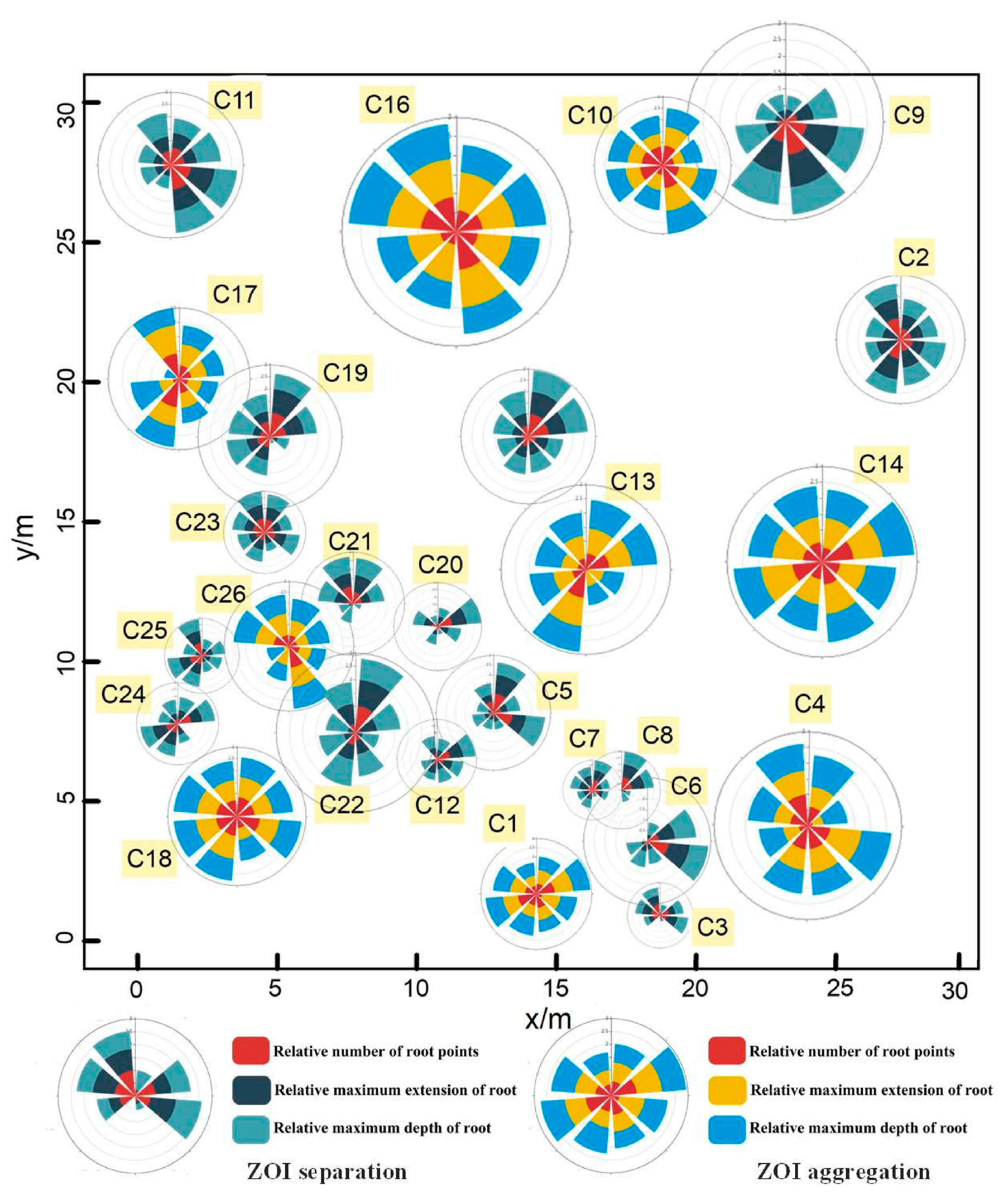
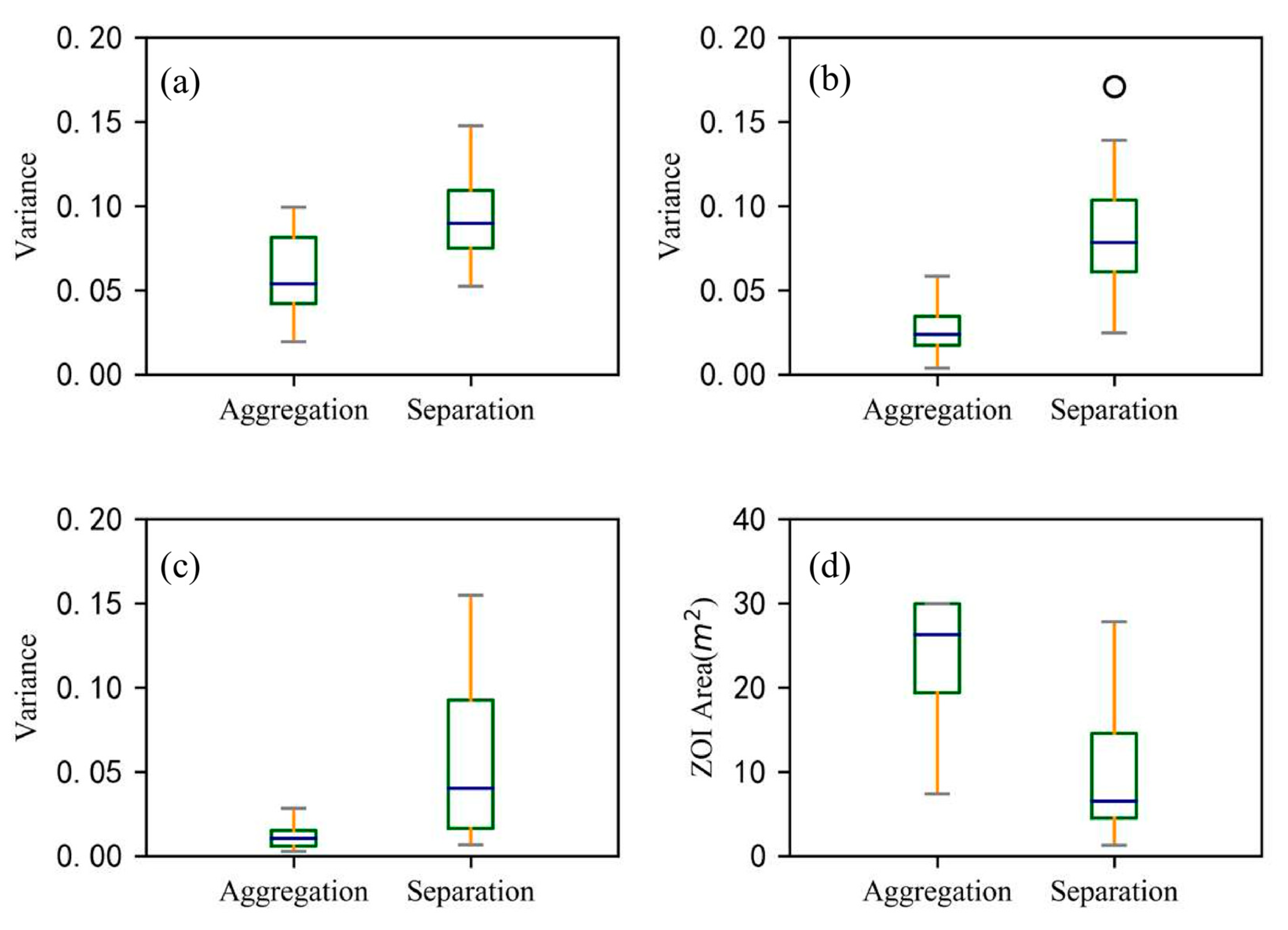
3.3. Characteristics of ZOI

Since the ZOIs at Site A could yield separated ZOIs (i.e., that each shrub has its own ZOI) or aggregated ZOIs (i.e., that multiple plants share the same ZOI), we used the Nightingale’s rose diagrams to quantify the degree of asymmetry in each ZOI in eight directions to compare the differences between the two types of ZOIs (i.e., separated ZOIs versus aggregated ZOIs). In general, root systems in each ZOI are distributing asymmetrically, occupying spaces in different directions. As shown in Figure 10 and Figure 11, the two ZOIs have apparent differences in size and shape, and the aggregated ZOI is larger and more symmetrical than the separated ZOI. The mean values of three parameters (i.e., the variance of the number of root points, the variance of root extension distance, and the variance of root depth) in eight directions of the separated ZOI are much larger than the mean values of these parameters of the aggregated ZOI, which proves that the separated ZOI is more asymmetrical than the aggregated ZOI. The mean value of the projected area for the separated ZOI is three times that of the aggregated ZOI.

4. Discussion

4.1. Advantages and Applicability of the Method

Since a plant’s ZOI is a key factor in the interactions within plant communities [6], the ability to quantify the sizes and shapes of ZOIs in the field helps us understand macroscopic plant interactions under different growth environments [41]. We achieved good results with the hierarchical clustering method (HDBSCAN) that we used to determine the sizes and shapes of plant ZOIs based on the root points of naturally growing C. microphylla shrubs detected by GPR surveys. These satisfactory ZOI results may be attributed to: (1) accurate root points detected by the GPR survey and (2) good extraction of the ZOIs using the effective hierarchical clustering method. The effectiveness of GPR in the identification and localization of plant roots has been demonstrated in previous studies [19,32]. With the advantages of good target positioning accuracy, high resolution, and non-destructive detection, GPR surveys provide the technical means to efficiently and accurately reveal the spatial distribution of belowground roots on a large scale. The HDBSCAN algorithm complements the GPR survey technique as a means of characterizing the ZOIs. Our results confirm that the distribution of roots in all directions around the plant is usually uneven (Figure 6a), as well as extremely irregular ZOI shapes [6,9,10,11,12,15]. Moreover, we found two different modes of ZOI and characterized their asymmetry, which is a result not obtained in previous studies. In short, applying the HDBSCAN algorithm to root points detected by GPR proved to be a promising approach to generating satisfactory ZOI results for shrubs.

We explored the impact that the numbers and spatial distributions of root points detected by GPR had on the applicability of HDBSCAN in the extraction of ZOI. As the interval between the survey lines increased, the number of root points detected by GPR dropped dramatically. More information about a root system can be retrieved with denser lines, which was beneficial for the extraction of ZOIs (Figure 8). However, decreasing the interval of survey lines requires more scans, leading to low-efficiency data collection, which hampers the application in large-scale studies. Moreover, intensive surveys may also cause root-point information duplication, resulting in data redundancies. By contrast, if the survey line interval is too large, the acquired information may be too sparse to be used to represent the actual distribution of the root system or ZOIs. A reasonable selection of the survey line interval should consider the tradeoff among the size of the research area, the radar antenna frequency, and the root growth characteristics of the studied plants. We recommend pre-experimental surveys in a small area to determine the optimal GPR deployment. The survey direction used on the simulation data (Figure 9) only had a slight impact on root detection and the ZOI results. This result demonstrates that changing the line direction only shifted the specific point positions of detected roots rather than their densities or clustering patterns. The experimental results of the simulated data further demonstrated our method’s stability and robustness for ZOI extraction.

4.2. Characteristics of ZOIs on the C. microphylla Population Scale

We identified two types of ZOIs: separated and aggregated ZOIs. The former is characterized by a shrub with its own ZOI that is completely separated from other ZOIs; the latter is characterized by multiple plants whose sub-ZOIs could not be distinguished and therefore shares the same ZOI. These two types of ZOIs are generally regarded as responses of plant roots to interactions with the roots of neighboring plants. For example, root system separation (i.e., separated ZOIs) has been confirmed in existing studies [11,42,43,44,45] and is mainly caused by two types of plant behavior: territorial behavior, in which plants occupy specific space resources and exclude root invasion from adjacent plants [46]; and evasive behavior, in which roots are distributed in the areas with the lowest competition for resources [47,48]. Other studies have also observed and explained the occurrence of root system aggregation (i.e., aggregated ZOIs) between neighboring plants [49,50,51]. In response to the competition for limited resources, plants may increase the size and extent of their own root systems to seize more resources, a response that often decreases the yield or biomass of the community as a whole [52]. In addition to competition, aggregation of roots may be driven by other factors, such as symbiosis between neighboring species, the plants’ reproductive strategies, and the ecological environment [53,54]. Our results indicate that a single species may engage in both of these distinct phenomena even within the same ecosystem, depending on site-specific conditions. The complex underground distribution patterns of the root systems of naturally growing communities or populations result from many factors, including competition, available nutrition, soil heterogeneity, species categories and quantities, and ecological environment. Our findings highlight the importance of considering various factors to explain the ZOIs as they respond to differences in the relative importance of the growth time, spatial structure, and various influencing factors.

The sizes and shapes of ZOIs are specific manifestations of the complexity of the spatial distribution patterns of roots [55]. Based on these characteristics, it is possible to analyze the influencing factors, including the interactions among plants and soil resources and between plants and other plants. Our results show that the shapes of the ZOIs are very irregular, which is consistent with the results of previous studies [7,11]. Some studies have shown that, for woody plants, the shape of the root system obtained by the whole root excavation method is usually an irregular polygon, which is likely the result of the heterogeneous distribution of resources in the soil or roots’ interactions with the roots of neighboring plants [6,56].

The rose diagrams showed that the two types of ZOIs differed considerably in both shape and size (Figure 10 and Figure 11), with the aggregated ZOIs being more extensive and more symmetrical than the separated ZOIs, likely caused by competition and compensatory growth of roots. Aggregated ZOIs have internal competition, and their main growth strategy is to occupy more soil to obtain resources, so the average projected area is more significant [46]. The separated ZOIs suffer less competitive, and the main growth strategy is to preferentially grow to places with richer resources, so they are more asymmetric [57]. Quantitative analysis of the size, shape, and plasticity of ZOIs may help us understand plant communities’ interactions, which may be more illustrative than just measuring parameters such as the root biomass or root:shoot ratio [6]. Further quantifications of ZOI characteristics, and analyses of the factors affecting root distribution patterns, will be essential contents of our following research. We expect to obtain quantitative expressions for some of the influencing factors on this basis and apply those results to predictive models of plant root traits and functions.

4.3. Limitations of this Method

Although GPR is very effective in root detection, it still misses small roots and deep roots. Guo et al. [32] reviewed in detail the penetration depth and root diameter of GPR in different species (please see the

Table A1. The maximum effective detection depth and minimum detectable root size of GPR systems with different radar frequencies used for root detection in various soil types [32].

Antenna Frequency (MHz)	Soil Type	Soil Texture		Soil Drainage Condition	Plant Species	Maximum Detection Depth (m)	Minimum Detectable Root Diameter (cm)	Reference
		Sand (%)	Clay and Silt (%)
250	-	-	-	Poor	Colophospermum mopane	4.00	-	Schoor and Colvin [61]
400	Gergeville soil	65	35	Well	Pinus taeda	1.00	3.7	Butnor et al. [19]
400	Lynchburg soil	70	30	Poor	Pinus taeda	1.30	-	Butnor et al. [19]
450	Loamy deluvium soil	30–60	40–70	Well	Quercus petraea	2.20	3.0–4.0	Hruška et al. [20]
450	Loess-Clay soil	<50 *	>50 *	Poor	Acer campestre	2.00	2.0–3.0	Čermák et al. [62]
450	Loess-Clay soil	<50 *	>50*	Well	Pinus nigra	2.50	2	Stokes et al. [63]
500	River sand	100 *	0 *	Well	Eucalyptus sp.	-	1	Barton and Montagub [35]
800	River sand	100 *	0 *	Well	Eucalyptus sp.	1.55	<1.0	Barton and Montagu [35]
900	Loamy sand	92	7	-	Prunus persica	1.14	2.5	Cox et al. [37]
900	Loamy sand	85	15	-	Prunus persica	-	1.2	Cox et al. [37]
900	Sand	100 *	0 *	Poor	Cryptomeria japonica	-	1.1	Dannoura et al. [64]
900	Sand	100 *	0 *	Well	Cryptomeria japonica	0.80	1.9	Hirano et al. [58]
1000	River sand	100 *	0 *	Well	Eucalyptus sp.	1.55	<1.0	Barton and Montagu [35]
1500	Sand	100 *	0 *	Well	-	-	0.25	Wielopolski et al. [65]
1500	Lakeland soil	90	10	Well	Populus deltoides	0.45	0.6	Butnor et al. [19]
1500	Wakulla soil	85–92	8–15	Well	Pinus taeda	0.50	0.5	Butnor et al. [19]
1500	Gergeville soil	65	35	Well	Pinus taeda	0.60	-	Butnor et al. [19]
1500	Troup and Lucy soil	>70 *	<30 *	Well	Pinus taeda	0.50	0.5	Butnor et al. [36]
1500	Sandy Pomello soil	>90 *	<10 *	Well	Quercus sp	0.60	0.5	Stover et al. [66]
2000	Sand	95	5	Well	Ulmus pumila	0.80	0.5	Cui et al. [59]

Those labeled with * are speculated values according to the corresponding soil types.

). Hruska et al. [20] used an EKKO 1000 GPR system with a 450 MHz frequency antenna to map the root distribution of a 50-year-old oak forest. They found that roots with diameters larger than 3 cm and the maximum depth of 2 meters were successfully detected by the selected GPR system. Hirano et al. [58] indicated that roots greater than 1.9 cm in diameter were clearly detected in the sand at a depth of 1m using 900 MHz GPR. Cui et al. [22] compared the profile excavation and the GPR measurement results, which indicated that the 400 and 900 MHz GPR could detect roots with a diameter greater than 0.5 cm under ideal conditions. Further, Cui et al. [22] found that the higher wave speed and lower GPR energy attenuation in frozen soil enhance the detection capability of deep coarse roots and, thus, advocated following studies combining seasonal GPR detection results to further enhance GPR-based root detection and quantification. Guo et al. [32] reviewed in detail the penetration depth and root diameter of GPR in different species. Although GPR is effective in root detection, it still misses small roots and deep roots. As coarse roots provide the framework for the attachment and growth of fine roots, they determine the expansion range of the whole root system. Therefore, the ZOIs extracted by this method should be similar to the actual ZOIs in shape, but the range is likely reduced.

Many studies have proved that soil moisture and soil texture will influence the effectiveness of coarse root detection by GPR [19,58,59]. Butnor et al. found that GPR is ineffective in soils with high clay or water content [19]. Most successful applications of GPR to measure roots were achieved when soil moisture was less than 15% [20,22]. In addition, the soil texture (e.g., and clay content) impacts the GPR identification of roots [38]. For example, Butnor et al. [19] found that GPR resolution was the best in dry sandy soils but seriously degraded in soils with moist clay contents. The clutter noise caused by the inhomogeneity of the soil background also interferes with the hyperbolic reflection of the root system and impairs the effectiveness of GPR in detecting roots [38]. Our study area is located in a desert steppe region of northern China, where the soil is mainly sand (~80% sand and ~20% silt and clay), and soil moisture generally keeps in a low level around 5~10%. This is an ideal condition for GPR root detection.

It should be mentioned that the simulated GPR root detection dataset has some limitations: (1) the inclined root will be projected as the lateral root in the process of simulated image mapping, which may cause incomplete signals and difficult recognition during field GPR surveys [32]; (2) the simulated dataset does not describe the variation of root diameter, which will affect the identification of GPR in actual applications; and (3) the results of root identification are affected by complex underground conditions in the field GPR measurement, including root size, root depth, soil moisture, and soil texture [21], which are not included in the simulation dataset. These factors impact the GPR signal strength and completeness and ultimately affect the generation of ZOIs. Therefore, large-scale validation of the proposed method in the field is still needed.

The HDBSCAN clustering algorithm also presents some challenges and limitations for the extraction of ZOIs. First, a multi-value test of the critical parameter k is required to adjust the parameter when using the HDBSCAN algorithm for density clustering analysis. GPR has a high detection accuracy for root systems [32] and obtains few non-root points (i.e., noise), so the selection of the k value tends to discard small noise points. The selection of the minimum cluster size (m) should also be determined using the input data. If this parameter is too small, there might be many pseudo sub-ZOIs split from the actual ZOIs, which would interfere with subsequent analysis. In contrast, if this parameter is too large, many root points might be errantly discarded as noise. Therefore, it is necessary to combine the characteristics of the research data with specific empirical rules to help assign appropriate values of k and m for practical applications. Further, the adaptive ability of the HDBSCAN hierarchy is limited: ZOIs with especially low densities may be removed as noise when the range of densities among the ZOIs is too wide (i.e., if the densest ZOI is approximately five times as dense as the most sparse ZOI) [60]. When the study area becomes large and with many species types distributing, the patterns of root system distribution will likely be more complicated. In such a case, the study area should be segmented according to the variation range in the root density, and the algorithm parameters of the segmented areas should be tuned carefully.

5. Conclusions

Plant ZOI is critical for studying the mechanisms of root–root and root–soil interactions. This study proposed a new method to reveal the ZOIs within a natural community of C. microphylla shrubs. First, GPR surveys were conducted to nondestructively map the spatial distribution of coarse roots. Then, the HDBSCAN algorithm was applied to the root points detected by GPR to perform an automatic cluster analysis, which determined the ZOIs of different shrubs. Finally, detailed information of each ZOI, such as its size and shape, was extracted and compared. The results of clustering roots into different ZOIs were validated in three ways. (1) The on-site excavation in the small area showed that belowground roots are intertwined and cannot be separated, which is the same as the ZOI patterns (both size and shape) derived from the root points detected by GPR. (2) The proposed method was tested in a simulated GPR root detection dataset on the medium spatial scale. The results indicate that most of the obtained ZOI patterns were in good agreement with the actual distribution of the root systems observed after excavation. Moreover, the way of setting up the GPR grids had limited influence on mapping ZOI by the HDBSCAN algorithm. (3) The proposed method was examined under the field condition in a larger area, and the Nightingale’s rose diagram was used to extract the size and shape of each ZOI. The ZOI determined based on root points detected by GPR demonstrated the natural growing pattern of roots, also confirming the effectiveness of the method. According to our results, the belowground distribution of the root system of C. microphylla was much larger than that of its aboveground canopy, and different shrub roots exhibited separated or aggregated ZOIs, accentuating the complexity of root growth in a natural community of C. microphylla. In addition, we found that aggregated ZOIs were less irregular in shape and occupied larger spatial areas than separated ZOIs. Based on these results, the integration of GPR root detection and HDBSCAN opens a new opportunity to study factors influencing ZOIs, such as the competition among plants, nutrient status, soil heterogeneity, and ecological environment.

References

1. Deans, J. Dynamics of coarse root production in a young plantation of Picea sitchensis. Forestry 1981, 54, 139–155. [Google Scholar] [CrossRef]
2. Reubens, B.; Poesen, J.; Danjon, F.; Geudens, G.; Muys, B. The role of fine and coarse roots in shallow slope stability and soil erosion control with a focus on root system architecture: A review. Trees 2007, 21, 385–402. [Google Scholar] [CrossRef]
3. Casper, B.B.; Jackson, R.B. Plant competition underground. Annu. Rev. Ecol. Evol. Syst. 1997, 28, 545–570. [Google Scholar] [CrossRef] [Green Version]
4. Wang, P.; Mou, P.; Li, Y.-B. Review of root nutrient foraging plasticity and root competition of plants. Chin. J. Plant Ecol. 2012, 36, 1184. [Google Scholar] [CrossRef]
5. Schenk, H.J. Root competition: Beyond resource depletion. J. Ecol. 2006, 94, 725–739. [Google Scholar] [CrossRef]
6. Casper, B.B.; Schenk, H.J.; Jackson, R.B. Defining a plant’s belowground zone of influence. Ecology 2003, 84, 2313–2321. [Google Scholar] [CrossRef]
7. Mou, P.; Mitchell, R.J.; Jones, R.H. Ecological field theory model: A mechanistic approach to simulate plant–plant interactions in southeastern forest ecosystems. Can. J. For. Res. 1993, 23, 2180–2193. [Google Scholar] [CrossRef]
8. Biondini, M.E.; Grygiel, C.E. Landscape distribution of organisms and the scaling of soil resources. Am. Nat. 1994, 143, 1026–1054. [Google Scholar] [CrossRef]
9. Bella, I.E. A new competition model for individual trees. For. Sci. 1971, 17, 364–372. [Google Scholar]
10. Berger, U.; Hildenbrandt, H. A new approach to spatially explicit modelling of forest dynamics: Spacing, ageing and neighbourhood competition of mangrove trees. Ecol. Modell. 2000, 132, 287–302. [Google Scholar] [CrossRef]
11. Brisson, J.; Reynolds, J.F. The effect of neighbors on root distribution in a creosotebush (Larrea tridentata) population. Ecology 1994, 75, 1693–1702. [Google Scholar] [CrossRef]
12. Brisson, J.; Reynolds, J.F. Effects of Compensatory Growth On Populationprocesses: A Simulation Study. Ecology 1997, 78, 2378–2384. [Google Scholar] [CrossRef]
13. O’Brien, E.E.; Brown, J.S.; Moll, J.D. Roots in space: A spatially explicit model for below-ground competition in plants. Proc. R. Soc. B 2007, 274, 929–935. [Google Scholar] [CrossRef] [Green Version]
14. Martin, M.; Snaydon, R.; Drennan, D. Lithium as a non-radioactive tracer for roots of intercropped species. Plant Soil 1982, 64, 203–208. [Google Scholar] [CrossRef]
15. Schiffers, K.; Tielbörger, K.; Tietjen, B.; Jeltsch, F. Root plasticity buffers competition among plants: Theory meets experimental data. Ecology 2011, 92, 610–620. [Google Scholar] [CrossRef]
16. Kummerow, J.; Krause, D.; Jow, W. Root systems of chaparral shrubs. Oecologia 1977, 29, 163–177. [Google Scholar] [CrossRef] [PubMed]
17. Zenone, T.; Morelli, G.; Teobaldelli, M.; Fischanger, F.; Matteucci, M.; Sordini, M.; Armani, A.; Ferrè, C.; Chiti, T.; Seufert, G. Preliminary use of ground-penetrating radar and electrical resistivity tomography to study tree roots in pine forests and poplar plantations. Funct. Plant Biol. 2008, 35, 1047–1058. [Google Scholar] [CrossRef] [PubMed]
18. Daniels, D.J. Surface-Penetrating Radar. Electron. Commun. Eng. J. 1996, 8, 165–182. [Google Scholar] [CrossRef]
19. Butnor, J.R.; Doolittle, J.; Kress, L.; Cohen, S.; Johnsen, K.H. Use of ground-penetrating radar to study tree roots in the southeastern United States. Tree Physiol. 2001, 21, 1269–1278. [Google Scholar] [CrossRef] [Green Version]
20. Hruska, J.; Čermák, J.; Šustek, S. Mapping tree root systems with ground-penetrating radar. Tree Physiol. 1999, 19, 125–130. [Google Scholar] [CrossRef] [Green Version]
21. Wu, Y.; Guo, L.; Cui, X.; Chen, J.; Cao, X.; Lin, H. Ground-penetrating radar-based automatic reconstruction of three-dimensional coarse root system architecture. Plant Soil 2014, 383, 155–172. [Google Scholar] [CrossRef]
22. Cui, X.; Liu, X.; Cao, X.; Fan, B.; Zhang, Z.; Chen, J.; Chen, X.; Lin, H.; Guo, L. Pairing dual-frequency GPR in summer and winter enhances the detection and mapping of coarse roots in the semi-arid shrubland in China. Eur. J. Soil Biol. 2020, 71, 236–251. [Google Scholar] [CrossRef]
23. Rahman, M.F.; Liu, W.; Suhaim, S.B.; Thirumuruganathan, S.; Zhang, N.; Das, G. Hdbscan: Density based clustering over location based services. arXiv 2016, arXiv:1602.03730. [Google Scholar]
24. Campello, R.J.; Moulavi, D.; Zimek, A.; Sander, J. A framework for semi-supervised and unsupervised optimal extraction of clusters from hierarchies. Data Min. Knowl. Discov. 2013, 27, 344–371. [Google Scholar] [CrossRef]
25. Veerhoek, L. Clustering Satellite Data to Define Eutrophication Monitoring Zones Based on Chlorophyll-a Concentration. Bachelor’s Thesis, Delft University of Technology, Delft, The Netherlands, 2020. [Google Scholar]
26. Rosalina, E.; Salim, F.D.; Sellis, T. Automated density-based clustering of spatial urban data for interactive data exploration. In Proceedings of the 2017 IEEE Conference on Computer Communications Workshops (INFOCOM WKSHPS), Atlanta, GA, USA, 1–4 May 2017; pp. 295–300. [Google Scholar]
27. Lin, C.-H.; Hsu, K.-C.; Johnson, K.R.; Luby, M.; Fann, Y.C. Applying density-based outlier identifications using multiple datasets for validation of stroke clinical outcomes. Int. J. Med. Inform. 2019, 132, 103988. [Google Scholar] [CrossRef]
28. Gill, R.A.; Jackson, R.B. Global patterns of root turnover for terrestrial ecosystems. New Phytol. 2000, 147, 13–31. [Google Scholar] [CrossRef]
29. Niu, H.; Li, H.; Zhao, M.; Han, X.; Dong, X. Relationship between soil water content and vertical distribution of root system under different ground water gradients in Maowusu Sandy Land. J. Arid Land Resour. Environ. 2008, 22, 157–163. [Google Scholar]
30. Wang, J.; Guo, Y.; Yao, Y.; Tang, J.; Zhang, M. Distribution characteristics of root system and carbon stock of Caragana microphylla Lam. in Aohan sandificational area. J. Northwest A F Univ. 2017, 45, 103–110. [Google Scholar]
31. Alamusa, J.D.; Tiefan, P. Soil moisture infiltration dynamics in plantation of Caragana microphylla in Heerqin sandy land. Chin. J. Ecol. 2004, 1, 56. [Google Scholar]
32. Guo, L.; Chen, J.; Cui, X.; Fan, B.; Lin, H. Application of ground penetrating radar for coarse root detection and quantification: A review. Plant Soil 2013, 362, 1–23. [Google Scholar] [CrossRef] [Green Version]
33. Murray, C.; Keiswetter, D. Application of magnetic and multi-frequency EM techniques for landfill investigations: Case histories. In Proceedings of the 11th EEGS Symposium on the Application of Geophysics to Engineering and Environmental Problems, Chicago, IL, USA, 22–26 March 1998; p. cp-203-00047. [Google Scholar]
34. Sato, T.; Takada, K.; Wakayama, T.; Kimura, I.; Abe, T.; Shinbo, T. Automatic data processing procedure for ground probing radar. IEICE Trans. Commun. 1994, 77, 831–837. [Google Scholar]
35. Barton, C.V.; Montagu, K.D. Detection of tree roots and determination of root diameters by ground penetrating radar under optimal conditions. Tree Physiol. 2004, 24, 1323–1331. [Google Scholar] [CrossRef] [PubMed] [Green Version]
36. Butnor, J.R.; Doolittle, J.; Johnsen, K.H.; Samuelson, L.; Stokes, T.; Kress, L. Utility of ground-penetrating radar as a root biomass survey tool in forest systems. Soil Sci. Soc. Am. J. 2003, 67, 1607–1615. [Google Scholar] [CrossRef] [Green Version]
37. Cox, K.; Scherm, H.; Serman, N. Ground-penetrating radar to detect and quantify residual root fragments following peach orchard clearing. HortTechnology 2005, 15, 600–607. [Google Scholar] [CrossRef]
38. Li, W.; Cui, X.; Guo, L.; Chen, J.; Chen, X.; Cao, X. Tree root automatic recognition in ground penetrating radar profiles based on randomized Hough transform. Remote Sens. 2016, 8, 430. [Google Scholar] [CrossRef] [Green Version]
39. McInnes, L.; Healy, J.; Astels, S. hdbscan: Hierarchical density based clustering. J. Open Res. Softw. 2017, 2, 205. [Google Scholar] [CrossRef]
40. Eldridge, J.; Belkin, M.; Wang, Y. Beyond hartigan consistency: Merge distortion metric for hierarchical clustering. In Proceedings of the Conference on Learning Theory, Paris, France, 3–6 July 2015; pp. 588–606. [Google Scholar]
41. Faget, M.; Nagel, K.A.; Walter, A.; Herrera, J.M.; Jahnke, S.; Schurr, U.; Temperton, V.M. Root–root interactions: Extending our perspective to be more inclusive of the range of theories in ecology and agriculture using in-vivo analyses. Ann. Bot. 2013, 112, 253–266. [Google Scholar] [CrossRef] [Green Version]
42. Gupta, P.; Rustgi, S. Molecular markers from the transcribed/expressed region of the genome in higher plants. Funct. Integr. Genomics. 2004, 4, 139–162. [Google Scholar] [CrossRef] [PubMed]
43. Mahall, B.E.; Callaway, R.M. Root communication among desert shrubs. Proc. Natl. Acad. Sci. USA 1991, 88, 874–876. [Google Scholar] [CrossRef] [Green Version]
44. Schmid, C.; Bauer, S.; Müller, B.; Bartelheimer, M. Belowground neighbor perception in Arabidopsis thaliana studied by transcriptome analysis: Roots of Hieracium pilosella cause biotic stress. Front. Plant Sci. 2013, 4, 296. [Google Scholar] [CrossRef] [Green Version]
45. Semchenko, M.; Zobel, K.; Heinemeyer, A.; Hutchings, M.J. Foraging for space and avoidance of physical obstructions by plant roots: A comparative study of grasses from contrasting habitats. New Phytol. 2008, 179, 1162–1170. [Google Scholar] [CrossRef] [PubMed]
46. Schenk, H.J.; Callaway, R.M.; Mahall, B. Spatial root segregation: Are plants territorial? In Advances in Ecological Research; Elsevier: Amsterdam, The Netherlands, 1999; Volume 28, pp. 145–180. [Google Scholar]
47. Zahavi, A.; Zahavi, A. The Handicap Principle: A Missing Piece of Darwin’s Puzzle; Oxford University Press: Oxford, UK, 1999. [Google Scholar]
48. Schenk, H.J.; Seabloom, E.W. Evolutionary ecology of plant signals and toxins: A conceptual framework. In Plant Communication from an Ecological Perspective; Springer: Berlin/Heidelberg, Germany, 2010; pp. 1–19. [Google Scholar]
49. Bartelheimer, M.; Steinlein, T.; Beyschlag, W. Aggregative root placement: A feature during interspecific competition in inland sand-dune habitats. Plant Soil 2006, 280, 101–114. [Google Scholar] [CrossRef]
50. Semchenko, M.; John, E.A.; Hutchings, M.J. Effects of physical connection and genetic identity of neighbouring ramets on root-placement patterns in two clonal species. New Phytol. 2007, 176, 644–654. [Google Scholar] [CrossRef]
51. Caffaro, M.M.; Vivanco, J.M.; Botto, J.; Rubio, G. Root architecture of Arabidopsis is affected by competition with neighbouring plants. Plant Growth Regul. 2013, 70, 141–147. [Google Scholar] [CrossRef]
52. Falik, O.; Reides, P.; Gersani, M.; Novoplansky, A. Root navigation by self inhibition. Plant Cell Environ. 2005, 28, 562–569. [Google Scholar] [CrossRef]
53. Schmid, C.; Bauer, S.; Bartelheimer, M. Should I stay or should I go? Roots segregate in response to competition intensity. Plant Soil 2015, 391, 283–291. [Google Scholar] [CrossRef]
54. Kiers, E.T.; Duhamel, M.; Beesetty, Y.; Mensah, J.A.; Franken, O.; Verbruggen, E.; Fellbaum, C.R.; Kowalchuk, G.A.; Hart, M.M.; Bago, A. Reciprocal rewards stabilize cooperation in the mycorrhizal symbiosis. Science 2011, 333, 880–882. [Google Scholar] [CrossRef] [Green Version]
55. Cabal, C.; Martínez-García, R.; de Castro Aguilar, A.; Valladares, F.; Pacala, S.W. The exploitative segregation of plant roots. Science 2020, 370, 1197–1199. [Google Scholar] [CrossRef]
56. Thomas, S.C.; Weiner, J. Including competitive asymmetry in measures of local interference in plant populations. Oecologia 1989, 80, 349–355. [Google Scholar] [CrossRef] [PubMed] [Green Version]
57. Ganatsas, P.; Spanos, I. Root system asymmetry of Mediterranean pines. In Eco-And Ground Bio-Engineering: The Use of Vegetation to Improve Slope Stability; Springer: Berlin/Heidelberg, Germany, 2007; pp. 127–134. [Google Scholar]
58. Hirano, Y.; Dannoura, M.; Aono, K.; Igarashi, T.; Ishii, M.; Yamase, K.; Makita, N.; Kanazawa, Y. Limiting factors in the detection of tree roots using ground-penetrating radar. Plant Soil 2009, 319, 15–24. [Google Scholar] [CrossRef]
59. Cui, X.; Chen, J.; Shen, J.; Cao, X.; Chen, X.; Zhu, X. Modeling tree root diameter and biomass by ground-penetrating radar. Sci. China Earth Sci. 2011, 54, 711–719. [Google Scholar] [CrossRef]
60. Malzer, C.; Baum, M. HDBSCAN (): An Alternative Cluster Extraction Method for HDBSCAN. arXiv 2019, arXiv:1911.02282. [Google Scholar]
61. Van Schoor, M.; Colvin, C. Tree root mapping with ground penetrating radar. In Proceedings of the 11th SAGA Biennial Technical Meeting and Exhibition, Swaziland, South Africa, 16–18 September 2009; p. cp-241-00077. [Google Scholar]
62. Cermak, J.; Hruska, J.; Martinkova, M.; Prax, A. Urban tree root systems and their survival near houses analyzed using ground penetrating radar and sap flow techniques. Plant Soil 2000, 219, 103–116. [Google Scholar] [CrossRef]
63. Stokes, A.; Fourcaud, T.; Hruska, J.; Cermak, J.; Nadyezdhina, N.; Nadyezhdin, V.; Praus, L. An evaluation of different methods to investigate root system architecture of urban trees in situ: I. Ground-penetrating radar. J. Arboric. 2002, 28, 2–10. [Google Scholar]
64. Dannoura, M.; Hirano, Y.; Igarashi, T.; Ishii, M.; Aono, K.; Yamase, K.; Kanazawa, Y. Detection of Cryptomeria japonica roots with ground penetrating radar. Plant Biosyst. 2008, 142, 375–380. [Google Scholar] [CrossRef]
65. Wielopolski, L.; Hendrey, G.; Daniels, J.J.; McGuigan, M. Imaging tree root systems in situ. In Proceedings of the Eighth International Conference on Ground Penetrating Radar, Gold Coast, Australia, 23–26 May 2000; pp. 642–646. [Google Scholar]
66. Stover, D.B.; Day, F.P.; Butnor, J.R.; Drake, B.G. Effect of elevated CO2 on coarse-root biomass in Florida scrub detected by ground-penetrating radar. Ecology 2007, 88, 1328–1334. [Google Scholar] [CrossRef] [Green Version]
Figure 1. Study area: (a) the location of field data collection; (b) satellite image of the study area; (c) schematic diagram of the ground-penetrating radar (GPR) survey line setting; (d) a field photo of Site A.
Remotesensing 13 01227 g001
Figure 2. Distribution of shrub crowns at Site A: the gray areas represent the crowns, and the white dots represent the center of each plant.
Remotesensing 13 01227 g002
Figure 3. An example of GPR data collection as well as identifying and locating root points in GPR images: (a) the GPR system used in this study; (b) a raw GPR image collected in the field before preprocessing; (c) the lateral coarse roots were located by identifying hyperbolic peaks in the GPR image collected over survey line No. 104 at Site A. Each peak of the hyperbola (indicated by the red dots) indicates the location of a root point.
Remotesensing 13 01227 g003
Figure 4. The procedure of applying the hierarchical density-based spatial clustering of applications with noise (HDBSCAN) algorithm: (a) root points detected by GPR; (b) the minimum spanning tree of mutually accessible distances; (c) hierarchy of the minimum spanning tree; (d) the condensed hierarchy; (e) clustering results extracted from the hierarchy.
Remotesensing 13 01227 g004
Figure 5. Simulated reference data: (a) the original reference data from an existing study [16]; (b) the processed root distribution map used to simulate roots that could be detected by GPR surveys. The dotted lines represent GPR survey lines with a 50 cm interval. The red stars represent the shrubs’ centers.
Remotesensing 13 01227 g005
Figure 6. The field survey and clustering results from Site A: (a) 2-D top view of the root distribution generated by GPR; (b) clustering results produced by the HDBSCAN algorithm. Different colors represent the root points of different zones of influence (ZOIs).
Remotesensing 13 01227 g006
Figure 7. The field survey and clustering results from Site B: (a) field photo; (b) 2-D top view of the distribution of root points interpreted from the GPR profile, in which the black dots represent the root points detected by GPR; (c) photo of the root systems after field excavation, in which each color represents the root system of the same shrub; (d) clustering results produced by the HDBSCAN algorithm. Different colors represent different ZOIs.
Remotesensing 13 01227 g007
Figure 8. Root points extracted by the simulated GPR survey and ZOI generated by the HDBSCAN algorithm at different line intervals: (a,e) 10 cm; (b,f) 15 cm; (c,g) 20 cm; (d,h) 25 cm. Different colors represent different ZOIs and are labeled with yellow labels. The red star points are the plants’ centers.
Remotesensing 13 01227 g008
Figure 9. Results after changing the survey line direction with the simulated data. The survey line interval was 10 cm. The results of the counterclockwise rotation of the survey line by 30°, 45°, and 60° are shown in (ac), respectively. The distribution maps of the corresponding ZOIs are in (df).
Remotesensing 13 01227 g009
Figure 10. Rose diagrams derived from the ZOIs. The rose diagrams are divided into three layers, representing the relative number of root points, the relative maximum extension of roots, and the relative maximum depth of the roots in the ZOI in eight directions. Different color bars represent different ZOI types. The centers of the rose diagrams of the separated ZOIs are based on the canopy centers, while the centers of the rose diagrams of the aggregated ZOIs are based on the center of the ZOIs (since multiple plants share the same ZOI).
Remotesensing 13 01227 g010
Figure 11. The degree of asymmetry of aggregated and separated ZOIs is indicated by the variances of three parameters: (a) the relative number of root points, (b) the relative maximum extension of a root, and (c) the relative maximum depth of roots. The three parameters of each ZOI were normalized. In addition, (d) the projected area of aggregated and separated ZOIs is shown. The line in the middle of the box represents the median value, and the upper and lower limits of the box are the upper quartile and the lower quartile, respectively. The whiskers represent the maximum and minimum values, except for outliers (circles).
Remotesensing 13 01227 g011
Publisher’s Note: MDPI stays neutral with regard to jurisdictional claims in published maps and institutional affiliations.