
Land Use and Land Cover Mapping Using RapidEye Imagery Based on a Novel Band Attention Deep Learning Method in the Three Gorges Reservoir Area


 , ,
, , 
Abstract
1. Introduction
- 1.
- We proposed an end-to-end deep learning method which overcame the limitations of traditional methods for high-resolution remote sensing classification.
- 2.
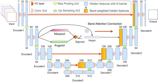
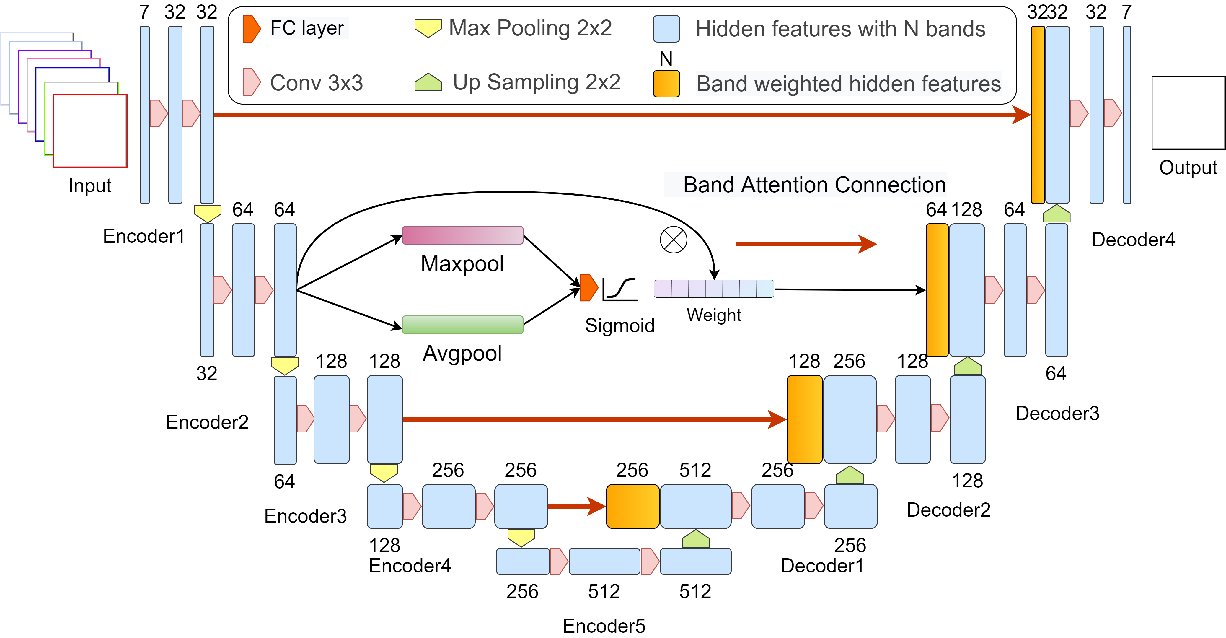
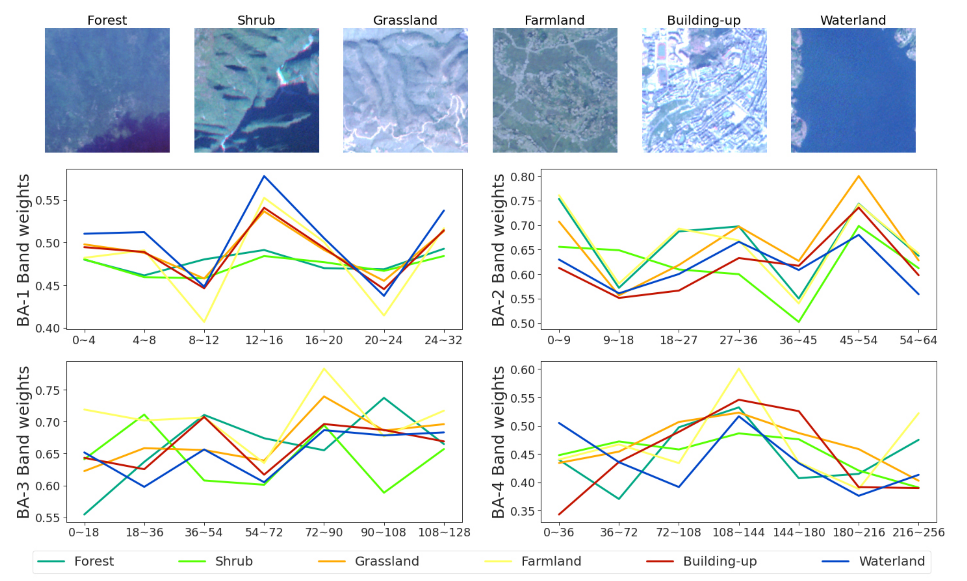
- We investigated the impact of the BA module on model performance which generated a dynamic weight for each band in CNN.
- 3.
- To evaluate the spatial generalizability of the proposed model, we tested the trained model at other regions of the study area.
2. Materials and Methods
2.1. Study Area
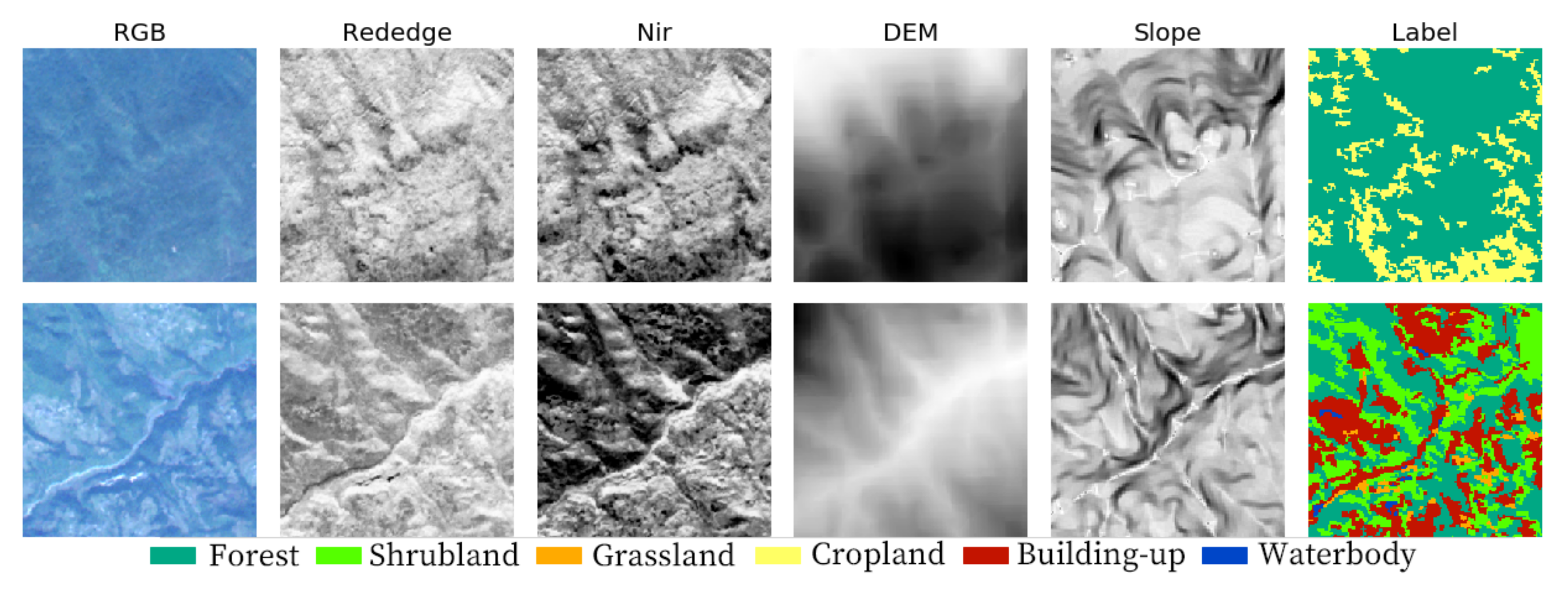
2.2. Data Sources
2.3. The Model Architecture
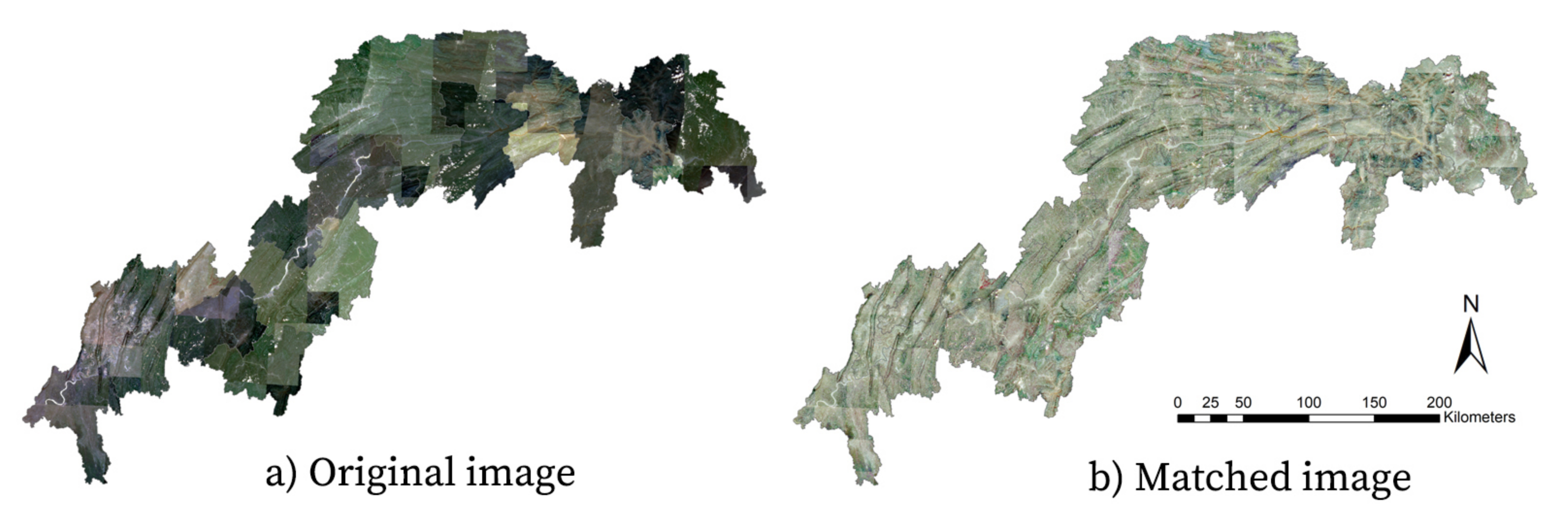
2.3.1. Data Preprocessing
2.3.2. Experiment Design
Models for Comparison
Accuracy Metrics
3. Results
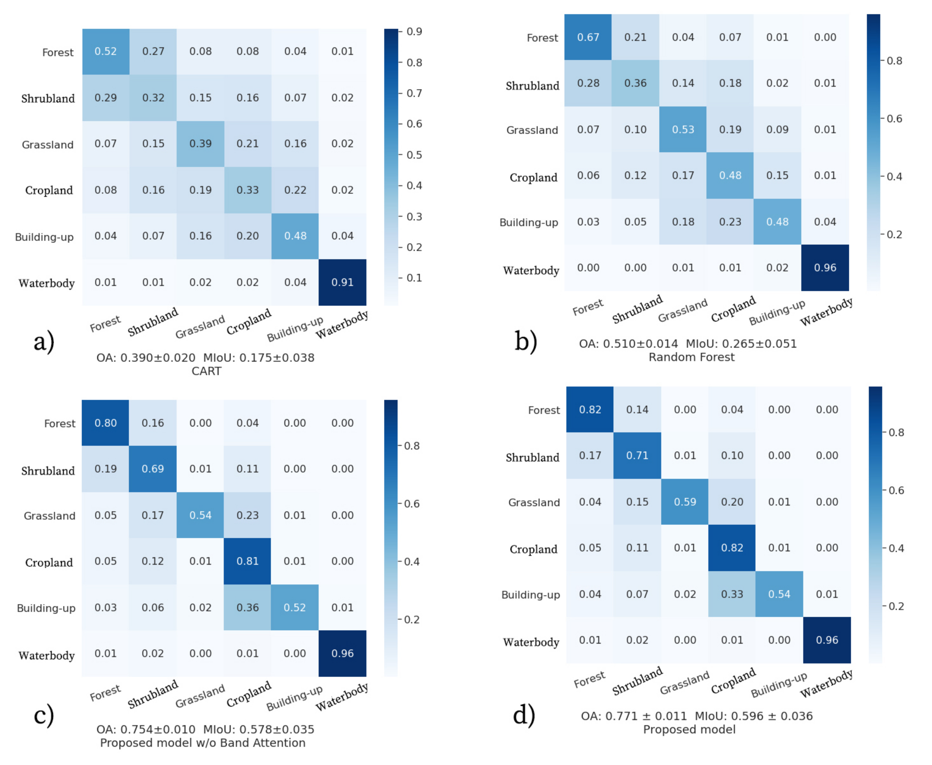
3.1. Classification Results
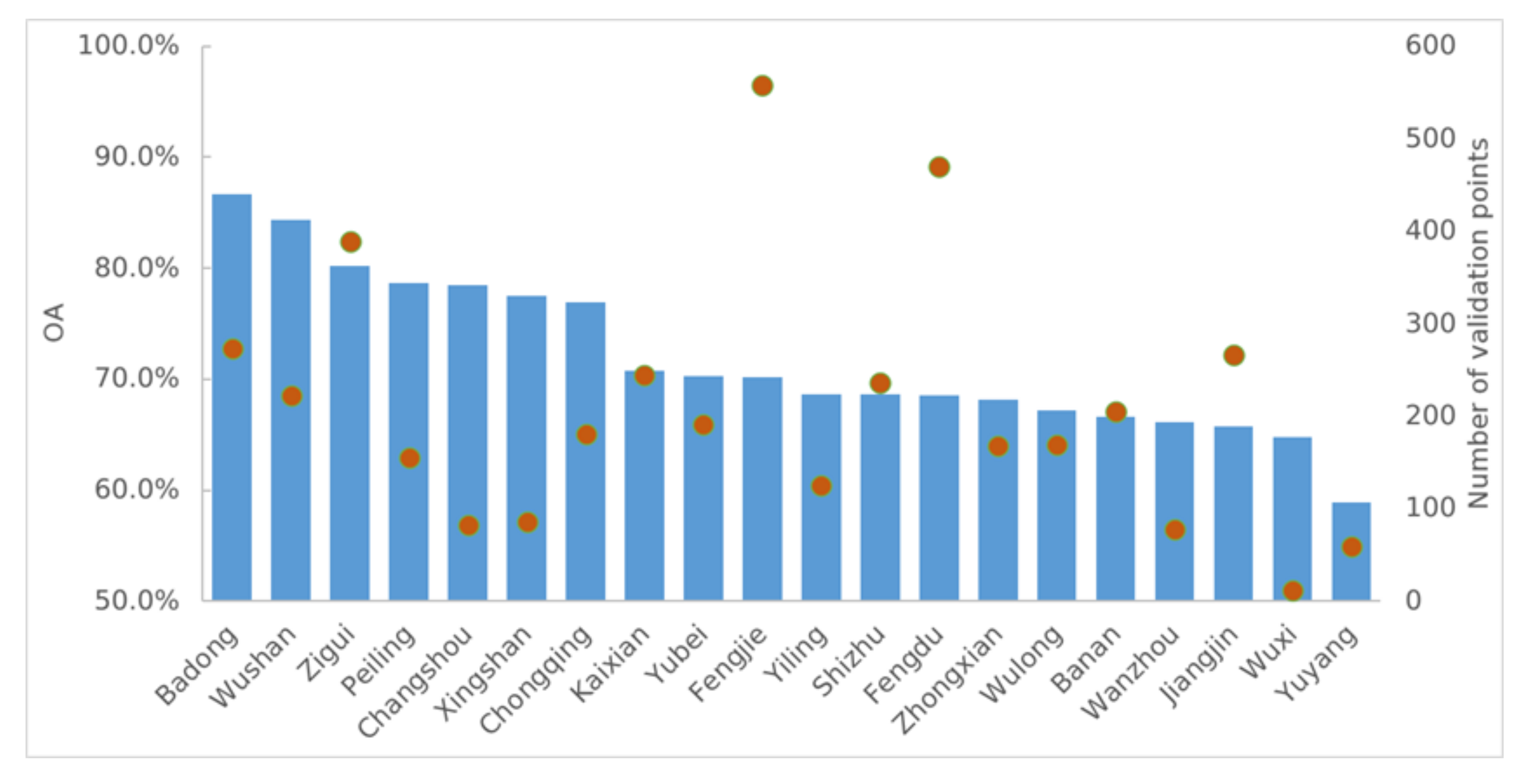
3.2. Model Generalizability
4. Discussion
4.1. Traditional Methods vs CNN Based Methods
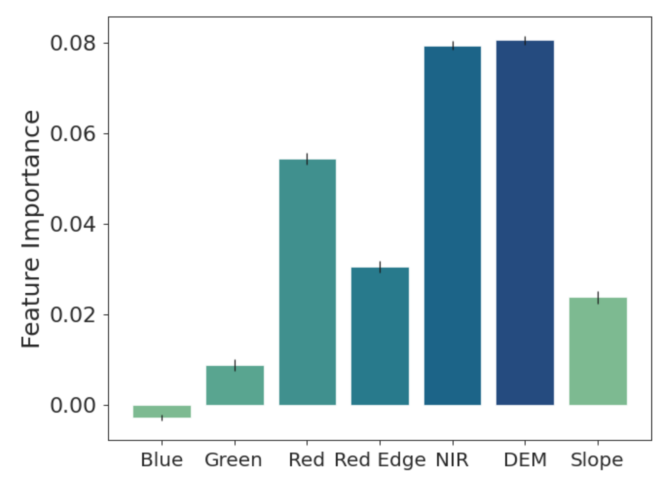
4.2. The Importance of Band Weighting
5. Conclusions
Author Contributions
Funding
Data Availability Statement
Acknowledgments
Conflicts of Interest
References
- Lei, Z.; Bingfang, W.; Liang, Z.; Peng, W. Patterns and driving forces of cropland changes in the Three Gorges Area, China. Reg. Environ. Chang. 2012, 12, 765–776. [Google Scholar] [CrossRef]
- Tullos, D. Assessing the influence of environmental impact assessments on science and policy: An analysis of the Three Gorges Project. J. Environ. Manag. 2009, 90, S208–S223. [Google Scholar] [CrossRef] [PubMed]
- Zhang, J.; Zhengjun, L.; Xiaoxia, S. Changing landscape in the Three Gorges Reservoir Area of Yangtze River from 1977 to 2005: Land use/land cover, vegetation cover changes estimated using multi-source satellite data. Int. J. Appl. Earth Obs. Geoinf. 2009, 11, 403–412. [Google Scholar] [CrossRef]
- Zhang, Q.; Lou, Z. The environmental changes and mitigation actions in the Three Gorges Reservoir region, China. Environ. Sci. Policy 2011, 14, 1132–1138. [Google Scholar] [CrossRef]
- Wu, J.; Huang, J.; Han, X.; Gao, X.; He, F.; Jiang, M.; Jiang, Z.; Primack, R.B.; Shen, Z. The three gorges dam: An ecological perspective. Front. Ecol. Environ. 2004, 2, 241–248. [Google Scholar] [CrossRef]
- Meyer, W.B.; Meyer, W.B.; BL Turner, I. Changes in Land Use And Land Cover: A Global Perspective; Cambridge University Press: Cambridge, UK, 1994; Volume 4. [Google Scholar]
- Pabi, O. Understanding land-use/cover change process for land and environmental resources use management policy in Ghana. GeoJournal 2007, 68, 369–383. [Google Scholar] [CrossRef]
- Gong, P.; Wang, J.; Yu, L.; Zhao, Y.; Zhao, Y.; Liang, L.; Niu, Z.; Huang, X.; Fu, H.; Liu, S.; et al. Finer resolution observation and monitoring of global land cover: First mapping results with Landsat TM and ETM+ data. Int. J. Remote. Sens. 2013, 34, 2607–2654. [Google Scholar] [CrossRef]
- Mora, B.; Tsendbazar, N.E.; Herold, M.; Arino, O. Global land cover mapping: Current status and future trends. In Land Use and Land Cover Mapping in Europe; Springer: Berlin/Heidelberg, Germany, 2014; pp. 11–30. [Google Scholar]
- Zhang, L.; Li, X.; Yuan, Q.; Liu, Y. Object-based approach to national land cover mapping using HJ satellite imagery. J. Appl. Remote. Sens. 2014, 8, 083686. [Google Scholar] [CrossRef]
- Zhang, X.; Han, L.; Han, L.; Zhu, L. How well do deep learning-based methods for land cover classification and object detection perform on high resolution remote sensing imagery? Remote. Sens. 2020, 12, 417. [Google Scholar] [CrossRef]
- Schowengerdt, R.A. Remote Sensing: Models and Methods for Image Processing; Elsevier: Amsterdam, The Netherlands, 2006. [Google Scholar]
- Yu, L.; Liang, L.; Wang, J.; Zhao, Y.; Cheng, Q.; Hu, L.; Liu, S.; Yu, L.; Wang, X.; Zhu, P.; et al. Meta-discoveries from a synthesis of satellite-based land-cover mapping research. Int. J. Remote. Sens. 2014, 35, 4573–4588. [Google Scholar] [CrossRef]
- Friedl, M.A.; Brodley, C.E. Decision tree classification of land cover from remotely sensed data. Remote. Sens. Environ. 1997, 61, 399–409. [Google Scholar] [CrossRef]
- Chasmer, L.; Hopkinson, C.; Veness, T.; Quinton, W.; Baltzer, J. A decision-tree classification for low-lying complex land cover types within the zone of discontinuous permafrost. Remote. Sens. Environ. 2014, 143, 73–84. [Google Scholar] [CrossRef]
- Hua, L.; Zhang, X.; Chen, X.; Yin, K.; Tang, L. A feature-based approach of decision tree classification to map time series urban land use and land cover with Landsat 5 TM and Landsat 8 OLI in a Coastal City, China. ISPRS Int. J. Geo-Inf. 2017, 6, 331. [Google Scholar] [CrossRef]
- Melgani, F.; Bruzzone, L. Classification of hyperspectral remote sensing images with support vector machines. IEEE Trans. Geosci. Remote. Sens. 2004, 42, 1778–1790. [Google Scholar] [CrossRef]
- Munoz-Marí, J.; Bovolo, F.; Gómez-Chova, L.; Bruzzone, L.; Camp-Valls, G. Semisupervised one-class support vector machines for classification of remote sensing data. IEEE Trans. Geosci. Remote. Sens. 2010, 48, 3188–3197. [Google Scholar] [CrossRef]
- Mountrakis, G.; Im, J.; Ogole, C. Support vector machines in remote sensing: A review. ISPRS J. Photogramm. Remote. Sens. 2011, 66, 247–259. [Google Scholar] [CrossRef]
- Belgiu, M.; Drăguţ, L. Random forest in remote sensing: A review of applications and future directions. ISPRS J. Photogramm. Remote. Sens. 2016, 114, 24–31. [Google Scholar] [CrossRef]
- Khatami, R.; Mountrakis, G.; Stehman, S.V. A meta-analysis of remote sensing research on supervised pixel-based land-cover image classification processes: General guidelines for practitioners and future research. Remote. Sens. Environ. 2016, 177, 89–100. [Google Scholar] [CrossRef]
- Jimenez-Rodriguez, L.O.; Rivera-Medina, J. Integration of spatial and spectral information in unsupervised classification for multispectral and hyperspectral data. In Image and Signal Processing for Remote Sensing V; International Society for Optics and Photonics: Bellingham, WA, USA, 1999; Volume 3871, pp. 24–33. [Google Scholar]
- Chen, Y.; Lin, Z.; Zhao, X.; Wang, G.; Gu, Y. Deep learning-based classification of hyperspectral data. IEEE J. Sel. Top. Appl. Earth Obs. Remote. Sens. 2014, 7, 2094–2107. [Google Scholar] [CrossRef]
- Huang, X.; Zhang, L. A multilevel decision fusion approach for urban mapping using very high-resolution multi/hyperspectral imagery. Int. J. Remote. Sens. 2012, 33, 3354–3372. [Google Scholar] [CrossRef]
- Chan, R.H.; Ho, C.W.; Nikolova, M. Salt-and-pepper noise removal by median-type noise detectors and detail-preserving regularization. IEEE Trans. Image Process. 2005, 14, 1479–1485. [Google Scholar] [CrossRef] [PubMed]
- Blaschke, T. Object based image analysis for remote sensing. ISPRS J. Photogramm. Remote. Sens. 2010, 65, 2–16. [Google Scholar] [CrossRef]
- Xiaoying, D. The application of ecognition in land use projects. Geomat. Spat. Inf. Technol. 2005, 28, 116–120. [Google Scholar]
- Burnett, C.; Blaschke, T. A multi-scale segmentation/object relationship modelling methodology for landscape analysis. Ecol. Model. 2003, 168, 233–249. [Google Scholar] [CrossRef]
- Benz, U.C.; Hofmann, P.; Willhauck, G.; Lingenfelder, I.; Heynen, M. Multi-resolution, object-oriented fuzzy analysis of remote sensing data for GIS-ready information. ISPRS J. Photogramm. Remote. Sens. 2004, 58, 239–258. [Google Scholar] [CrossRef]
- Tilton, J.C. Image segmentation by region growing and spectral clustering with a natural convergence criterion. In Proceedings of the IGARSS’98-Sensing and Managing the Environment-1998 IEEE International Geoscience and Remote Sensing, Symposium Proceedings (Cat. No. 98CH36174), Seattle, WA, USA, 6–10 July 1998; Volume 4, pp. 1766–1768. [Google Scholar]
- Tian, J.; Chen, D.M. Optimization in multi-scale segmentation of high-resolution satellite images for artificial feature recognition. Int. J. Remote. Sens. 2007, 28, 4625–4644. [Google Scholar] [CrossRef]
- Roerdink, J.B.; Meijster, A. The watershed transform: Definitions, algorithms and parallelization strategies. Fundam. Inform. 2000, 41, 187–228. [Google Scholar] [CrossRef]
- Audebert, N.; Le Saux, B.; Lefèvre, S. Semantic segmentation of earth observation data using multimodal and multi-scale deep networks. In Proceedings of the Asian Conference on Computer Vision, Taipei, Taiwan, 20–24 November 2016; pp. 180–196. [Google Scholar]
- Long, J.; Shelhamer, E.; Darrell, T. Fully convolutional networks for semantic segmentation. In Proceedings of the IEEE Conference on Computer Vision and Pattern Recognition, Boston, MA, USA, 7–12 June 2015; pp. 3431–3440. [Google Scholar]
- Badrinarayanan, V.; Handa, A.; Cipolla, R. Segnet: A Deep Convolutional Encoder-Decoder Architecture for Robust Semantic Pixel-Wise Labelling. arXiv 2015, arXiv:1505.07293. [Google Scholar]
- Ronneberger, O.; Fischer, P.; Brox, T. U-net: Convolutional networks for biomedical image segmentation. In Proceedings of the International Conference on Medical Image Computing and Computer-Assisted Intervention, Munich, Germany, 5–9 October 2015; pp. 234–241. [Google Scholar]
- Jégou, S.; Drozdzal, M.; Vazquez, D.; Romero, A.; Bengio, Y. The one hundred layers tiramisu: Fully convolutional densenets for semantic segmentation. In Proceedings of the IEEE Conference on Computer Vision and Pattern Recognition Workshops, Honolulu, HI, USA, 21–26 July 2017; pp. 11–19. [Google Scholar]
- Paszke, A.; Chaurasia, A.; Kim, S.; Culurciello, E. Enet: A Deep Neural Network Architecture for Real-Time Semantic Segmentation. arXiv 2016, arXiv:1606.02147. [Google Scholar]
- Chaurasia, A.; Culurciello, E. Linknet: Exploiting encoder representations for efficient semantic segmentation. In Proceedings of the 2017 IEEE Visual Communications and Image Processing (VCIP), St. Petersburg, FL, USA, 10–13 December 2017; pp. 1–4. [Google Scholar]
- Lin, G.; Milan, A.; Shen, C.; Reid, I. Refinenet: Multi-path refinement networks for high-resolution semantic segmentation. In Proceedings of the IEEE Conference on Computer Vision and Pattern Recognition, Honolulu, HI, USA, 21–26 July 2017; pp. 1925–1934. [Google Scholar]
- Zhao, H.; Shi, J.; Qi, X.; Wang, X.; Jia, J. Pyramid scene parsing network. In Proceedings of the IEEE Conference on Computer Vision and Pattern Recognition, Honolulu, HI, USA, 21–26 July 2017; pp. 2881–2890. [Google Scholar]
- Rouse, J.W.; Haas, R.H.; Schell, J.A.; Deering, D.W.; Harlan, J.C. Monitoring the Vernal Advancement and Retrogradation (Green Wave Effect) of Natural Vegetation; NASA/GSFC Type III Final Report; NASA: Greenbelt, MD, USA, 1974; Volume 371.
- Huete, A.R. A soil-adjusted vegetation index (SAVI). Remote. Sens. Environ. 1988, 25, 295–309. [Google Scholar] [CrossRef]
- Gao, B.C. NDWI—A normalized difference water index for remote sensing of vegetation liquid water from space. Remote. Sens. Environ. 1996, 58, 257–266. [Google Scholar] [CrossRef]
- De Sousa, C.; Souza, C.; Zanella, L.; De Carvalho, L. Analysis of RapidEye’s Red edge band for image segmentation and classification. In Proceedings of the 4th GEOBIA, Rio de Janeiro, Brazil, 7–9 May 2012; Volume 79, pp. 7–9. [Google Scholar]
- Kotchenova, S.Y.; Vermote, E.F.; Levy, R.; Lyapustin, A. Radiative transfer codes for atmospheric correction and aerosol retrieval: Intercomparison study. Appl. Opt. 2008, 47, 2215–2226. [Google Scholar] [CrossRef] [PubMed]
- Benediktsson, J.A.; Swain, P.H.; Ersoy, O.K. Neural Network Approaches Versus Statistical Methods in Classification of Multisource Remote Sensing Data. IEEE Trans. Geosci. Remote. Sens. 1990, 28, 540–552. [Google Scholar] [CrossRef]
- Farr, T.G.; Rosen, P.A.; Caro, E.; Crippen, R.; Duren, R.; Hensley, S.; Kobrick, M.; Paller, M.; Rodriguez, E.; Roth, L.; et al. The shuttle radar topography mission. Rev. Geophys. 2007, 45. [Google Scholar] [CrossRef]
- Burrough, P.A.; McDonnell, R.; McDonnell, R.A.; Lloyd, C.D. Principles of Geographical Information Systems; Oxford University Press: Oxford, UK, 2015. [Google Scholar]
- Fonarow, G.C.; Adams, K.F.; Abraham, W.T.; Yancy, C.W.; Boscardin, W.J.; ADHERE Scientific Advisory Committee. Risk stratification for in-hospital mortality in acutely decompensated heart failure: Classification and regression tree analysis. JAMA 2005, 293, 572–580. [Google Scholar] [CrossRef] [PubMed]
- Gao, W.; Zeng, Y.; Zhao, D.; Wu, B.; Ren, Z. Land Cover Changes and Drivers in the Water Source Area of the Middle Route of the South-to-North Water Diversion Project in China from 2000 to 2015. Chin. Geogr. Sci. 2020, 30, 115–126. [Google Scholar] [CrossRef]
- Zhang, X.; Wu, B.; Zhang, M.; Zeng, H. Mapping rice extent map with crop intensity in south China through integration of optical and microwave images based on google earth engine. In Proceedings of the AGU Fall Meeting, Washington, DC, USA, 11–15 December 2017; Volume 2017, p. B51C-1812. [Google Scholar]
- GVG—Apps on Google Play. Available online: https://play.google.com/store/apps/details?id=com.sysapk.gvg&hl=en_GB&gl=US (accessed on 28 December 2020).
- Xu, B.; Wang, N.; Chen, T.; Li, M. Empirical evaluation of rectified activations in convolutional network. arXiv 2015, arXiv:1505.00853. [Google Scholar]
- Ioffe, S.; Szegedy, C. Batch normalization: Accelerating deep network training by reducing internal covariate shift. In Proceedings of the International Conference on Machine Learning, Lille, France, 6–11 July 2015; pp. 448–456. [Google Scholar]
- Richards, J.A.; Richards, J. Remote Sensing Digital Image Analysis; Springer: Berlin/Heidelberg, Germany, 1999; Volume 3. [Google Scholar]
- Krizhevsky, A.; Sutskever, I.; Hinton, G.E. Imagenet classification with deep convolutional neural networks. Adv. Neural Inf. Process. Syst. 2012, 25, 1097–1105. [Google Scholar] [CrossRef]
- Pedregosa, F.; Varoquaux, G.; Gramfort, A.; Michel, V.; Thirion, B.; Grisel, O.; Blondel, M.; Prettenhofer, P.; Weiss, R.; Dubourg, V.; et al. Scikit-learn: Machine learning in Python. J. Mach. Learn. Res. 2011, 12, 2825–2830. [Google Scholar]
- Happ, P.; Ferreira, R.S.; Bentes, C.; Costa, G.; Feitosa, R.Q. Multiresolution segmentation: A parallel approach for high resolution image segmentation in multicore architectures. Int. Arch. Photogramm. Remote. Sens. Spat. Inf. Sci. 2010, 38, C7. [Google Scholar]


| Classifier | Parameters | Standardize Method |
|---|---|---|
| num_leaves = 20 | ||
| min_samples_leaf = 1 | ||
| min_samples_split = 2 | ||
| CART | degree = 3 | StandardScalerWrapper |
| gamma = auto_deprecated | ||
| max_iter = −1 | ||
| RF | n_estimators = 10 | |
| min_samples_leaf = 1 |
| Method | CART | RF | Proposed Model w/o BA | Proposed Model with BA |
|---|---|---|---|---|
| F1-Score ± Std | ||||
| Forest | 0.427 ± 0.028 | 0.667 ± 0.032 | 0.795 ± 0.017 | 0.811 ± 0.018 |
| Shrubland | 0.273 ± 0.021 | 0.427 ± 0.038 | 0.706 ± 0.026 | 0.731 ± 0.024 |
| Grassland | 0.204 ± 0.044 | 0.247 ± 0.030 | 0.585 ± 0.107 | 0.631 ± 0.099 |
| Cropland | 0.240 ± 0.041 | 0.488 ± 0.050 | 0.758 ± 0.018 | 0.767 ± 0.015 |
| Built-up | 0.260 ± 0.068 | 0.212 ± 0.018 | 0.549 ± 0.096 | 0.574 ± 0.074 |
| Waterbody | 0.842 ± 0.072 | 0.905 ± 0.003 | 0.907 ± 0.101 | 0.892 ± 0.118 |
| OA ± Std | 0.390 ± 0.020 | 0.510 ± 0.014 | 0.754 ± 0.010 | 0.771 ± 0.011 |
| MIoU ± Std | 0.175 ± 0.038 | 0.265 ± 0.051 | 0.578 ± 0.035 | 0.596 ± 0.036 |
Publisher’s Note: MDPI stays neutral with regard to jurisdictional claims in published maps and institutional affiliations. |
© 2021 by the authors. Licensee MDPI, Basel, Switzerland. This article is an open access article distributed under the terms and conditions of the Creative Commons Attribution (CC BY) license (http://creativecommons.org/licenses/by/4.0/).
Share and Cite
Zhang, X.; Du, L.; Tan, S.; Wu, F.; Zhu, L.; Zeng, Y.; Wu, B. Land Use and Land Cover Mapping Using RapidEye Imagery Based on a Novel Band Attention Deep Learning Method in the Three Gorges Reservoir Area. Remote Sens. 2021, 13, 1225. https://doi.org/10.3390/rs13061225
Zhang X, Du L, Tan S, Wu F, Zhu L, Zeng Y, Wu B. Land Use and Land Cover Mapping Using RapidEye Imagery Based on a Novel Band Attention Deep Learning Method in the Three Gorges Reservoir Area. Remote Sensing. 2021; 13(6):1225. https://doi.org/10.3390/rs13061225
Chicago/Turabian StyleZhang, Xin, Ling Du, Shen Tan, Fangming Wu, Liang Zhu, Yuan Zeng, and Bingfang Wu. 2021. "Land Use and Land Cover Mapping Using RapidEye Imagery Based on a Novel Band Attention Deep Learning Method in the Three Gorges Reservoir Area" Remote Sensing 13, no. 6: 1225. https://doi.org/10.3390/rs13061225
APA StyleZhang, X., Du, L., Tan, S., Wu, F., Zhu, L., Zeng, Y., & Wu, B. (2021). Land Use and Land Cover Mapping Using RapidEye Imagery Based on a Novel Band Attention Deep Learning Method in the Three Gorges Reservoir Area. Remote Sensing, 13(6), 1225. https://doi.org/10.3390/rs13061225