Abstract
Climate change is largely determined by the radiation budget imbalance at the Top Of the Atmosphere (TOA), which is generated by the increasing concentrations of greenhouse gases (GHGs). As a result, the Earth Energy Imbalance (EEI) is considered as an Essential Climate Variable (ECV) that has to be monitored continuously from space. However, accurate TOA radiation measurements remain very challenging. Ideally, EEI monitoring should be performed with a constellation of satellites in order to resolve as much as possible spatio-temporal fluctuations in EEI which contain important information on the underlying mechanisms driving climate change. The monitoring of EEI and its components (incoming solar, reflected solar, and terrestrial infrared fluxes) is the main objective of the UVSQ-SAT pathfinder nanosatellite, the first of its kind in the construction of a future constellation. UVSQ-SAT does not have an active determination system of its orientation with respect to the Sun and the Earth (i.e., the so-called attitude), a prerequisite in the calculation of EEI from the satellite radiation measurements. We present a new effective method to determine the UVSQ-SAT’s in-orbit attitude using its housekeeping and scientific sensors measurements and a well-established deep learning algorithm. One of the goals is to estimate the satellite attitude with a sufficient accuracy for retrieving the radiative fluxes (incoming solar, reflected solar, terrestrial infrared) on each face of the satellite with an uncertainty of less than ±5 Wm (1). This new method can be extended to any other satellites with no active attitude determination or control system. To test the accuracy of the method, a ground-based calibration experiment with different attitudes is performed using the Sun as the radiative flux reference. Based on the deep learning estimation of the satellite ground-based attitude, the uncertainty on the solar flux retrieval is about ±16 Wm (1). The quality of the retrieval is mainly limited by test conditions and the number of data samples used in training the deep learning system during the ground-based calibration. The expected increase in the number of training data samples will drastically decrease the uncertainty in the retrieved radiative fluxes. A very similar algorithm will be implemented and used in-orbit for UVSQ-SAT.
1. Introduction
UltraViolet & infrared Sensors at high Quantum efficiency on-board a small SATellite (UVSQ-SAT) is a pioneering space-based mission to demonstrate technologies for broadband measurements of Earth Radiation Budget (ERB) [1]. The mission is part of the International Satellite Program in Research and Education (INSPIRE). The motivation of the UVSQ-SAT mission (INSPIRE-05) is to implement miniaturized disruptive technologies for remote sensing with compact sensors that could be used in the future for a multi-point satellite constellation for observing Essential Climate Variables (ECV), namely shortwave and longwave radiative fluxes at the Top Of the Atmosphere (TOA) and UV solar spectral irradiance [2,3]. As a result of the increasing levels of infrared (IR) radiation-trapping greenhouse gases (GHGs), the global energy budget is not balanced with the excess energy accumulating in the Earth system. As a response, global mean surface temperatures increase in order to enhance the outgoing terrestrial IR radiation and thus restore the Earth energy balance. Measuring the absolute value of the Earth’s Energy Imbalance (EEI) and its variability over time appears to be a very difficult challenge. Indeed, EEI is a measure of the energy accumulation rate and hence of the warming trend of the Earth system. EEI is derived from the simultaneous measurements of its different components: incoming solar, reflected solar, and terrestrial infrared radiative fluxes. Ideally, EEI monitoring should be performed with a constellation of satellites in order to resolve as much as possible spatio-temporal fluctuations in EEI which are indicative of the underlying mechanisms driving climate change at global and regional scales. The relevant scientific goal is to be able to detect any EEI long-term trend with a target accuracy of 1/10 of the expected signal of 0.5–1.0 Wm in the global mean during a decade [4,5,6]. These EEI scientific objectives are extremely relevant and have not been achieved so far. At the present stage, the UVSQ-SAT CubeSat is a demonstrator, expecting future developments and improvements that would then really allow for making use of CubeSat technology for these scientific purposes. The expected performances for UVSQ-SAT are to measure the EEI with a stability per year of ±5 Wm at 1 [1]. The UVSQ-SAT EEI expected performances depend on the error budget of several parameters. The in-orbit attitude determination of the satellite is one of these parameters, which represents a random error. Thus, the accurate determination of the UVSQ-SAT CubeSat in-orbit attitude is essential and implies an EEI determination that should be less than ±5 Wm at 1.
To measure the EEI at the TOA, the UVSQ-SAT satellite has Earth Radiative Sensors (ERS) on each face of the CubeSat. The main goal of the UVSQ-SAT mission is to measure with accuracy the incoming solar radiation (Total Solar Irradiance (TSI)) and the Earth outgoing radiation (EOR = TOA Outgoing Longwave Radiation (OLR) + Shortwave Radiation (OSR)). There are two different strategies to measure and recover all Earth radiative fluxes (solar, albedo, infrared) from UVSQ-SAT sensors. The first one is to compute an average flux on the six different faces of the CubeSat as explained in details by [1]. However, this method implies identical responsivity and the same bidirectional reflectance distribution function (BRDF) for all sensors of all faces of the CubeSat. The second strategy is to compute the radiative fluxes (solar, albedo, infrared) for each face of the spacecraft. This method implies a good knowledge of the UVSQ-SAT’s in-orbit attitude. However, the UVSQ-SAT CubeSat does not have an attitude control system due to its compact design. Indeed, no instrument is integrated on-board the UVSQ-SAT CubeSat to determine its attitude (i.e., orientation in the reference frame) explicitly. For this reason, a new method based on a deep learning algorithm was developed to determine accurately the UVSQ-SAT in-orbit attitude using its on-board housekeeping and scientific sensors’ measurements. The method is first tested here against ground-based calibration data. The method will also be tested further in orbit. Ultimately, this approach for attitude determination could be applicable to all future small satellites with radiative and optical scientific sensors on several faces on the spacecraft but without the need for specific active on-board attitude determination equipments.
Different approaches can be implemented to determine the in-orbit attitude of a satellite. Satellite attitude determination and control system (ADCS) include sensors used to determine attitude and attitude rate, such as Sun sensors, horizon sensors, magnetometers, gyros and star trackers while actuators (magnetorquers, reaction wheels, thrusters) are designed to change the spacecraft’s attitude. All of these sensors are more or less accurate and all are different, as described in [7]. Sun sensors are used to provide an estimate of the solar location in the spacecraft body frame, which can be used to estimate satellite attitude (accuracy less than 1). Horizon sensors can be simple infrared horizon crossing indicators or more advanced thermopile sensors to detect the temperature differences between the poles and the equator (accuracy less than 1). Magnetometers provide a measurement of the local magnetic field used to provide both estimates of attitude and also orbital position. Star tracker can provide an accurate, standalone estimate of the spacecraft’s attitude by comparing a digital image captured with a CCD or CMOS sensor to an onboard star catalog. For three-axis-stabilized spacecraft missions using star trackers, the pointing accuracy can vary from 0.001 to approximately 0.7 at 1. For spin-stabilized spacecraft missions, the pointing accuracy vary from 0.2 to 1 at 1. These values correspond to the optimum conditions of use. In practice, many factors affect this accuracy, such as stray light and magnetic interference. Other spacecrafts use photocells or camera to detect stars or Earth [8] for attitude determination. Earth detection using real time image recognition in deep learning has been described to determine the attitude of a satellite in [9]. On the UVSQ-SAT satellite, no devices are present to perform image recognition to detect the Earth’s location. To determine the UVSQ-SAT’s in-orbit attitude, we will use housekeeping (temperatures sensors and solar photodiodes (400–1100 nm)) and scientific sensors (Earth Radiative sensors—thermopiles) measurements.
The main goal of this manuscript is to develop a new concept based on deep learning method to obtain the UVSQ-SAT in-orbit attitude to retrieve the different components of the EEI for each face of the spacecraft. To validate the method before launch, a ground-based calibration was carried out in Guyancourt (France) in October 2020. The Sun was used as radiative flux reference. The amount of calibration data acquired was limited due to the tight schedule and associated constraints (such as delay in integrations, bad weather conditions during the test period, delivery date to the launcher). One of the initial objectives was to validate new miniaturized technologies in orbit at technology readiness level of 9 (system proven in operational environment) in a short time frame program. An objective of UVSQ-SAT is to be able to learn from this first mission about the development of a future satellites constellation.
Section 2 gives a description of the deep learning method to retrieve the attitude of the UVSQ-SAT satellite and presents the ground-based validation process. This method allows for retrieving the attitude of a small spacecraft without any dedicated instrument to do so. This technique does not require to add a specific instrument. This is favorable as a small satellite tends to reduce the space needed along with the complexity of integrating one more instrument. Moreover, it will lower the data rate to provide. Deep learning algorithms are often used for remote sensing applications [10]. Neural networks are implemented using satellite data for detect farms or to classify lands as in [11,12,13,14]. This technique appears to be really convenient in the remote sensing field.
Section 3 presents the results and performance of the algorithm for the validation process.
Finally, Section 4 provides discussion and perspectives for in-orbit applications.
2. Method to Retrieve Terrestrial Net Radiation for Satellite That Does Not Have Active ADCS
The main goal of the UVSQ-SAT pathfinder mission is to determine the Terrestrial Net Radiation using remote sensors. The UVSQ-SAT CubeSat described in [1] has several sensors on its six different faces:
- 12 ERS sensors are part of the UVSQ-SAT satellite (2 per face). Six ERS sensors aims to measure radiation between 0.2 and 100 m using Carbon NanoTubes coatings (absorptivity close to 1). Six other ERS sensors aim to measure radiation wavelength between 0.2 and 3 m with 0.06 absorptivity and between 3 and 100 m with 0.84 absorptivity using optical solar reflector coatings. ERS measurements represent indicators to detect Earth and the Sun positions.
- Three ultraviolet sensors (UVS) are part of the UVSQ-SAT scientific payload. They focus on the 200–1100 nm wavelength range.
- Six photodiodes (LED) are located on the spacecraft and measure solar and outgoing shortwave radiations in the 400–1100 nm wavelength range.
- Temperature sensors (solar cells) are also located on each satellite panel.
- Teach’ Wear (TW) is a new three axis accelerometer/gyroscope/compass. The TW module on-board UVSQ-SAT has an instrumentation that will be very helpful to determine the reference position during the training phase such as: a three-axis accelerometer, a three-axis gyrometer, and a three-axis magnetometer.
In the case of a satellite such as UVSQ-SAT that does not have an active attitude determination and control system, it is necessary to develop a typical method to retrieve terrestrial net radiation.
2.1. General Method Description to Determine the Terrestrial Net Radiation
Figure 1 presents the general method to determine the terrestrial net radiation from the UVSQ-SAT satellite. The main goal is to obtain the incoming solar radiation (TSI), the Outgoing Longwave Radiation (OLR), and the Outgoing Shortwave Radiation (OSR) from the satellite measurements.
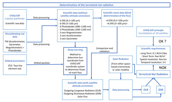
Figure 1.
General method to determine the terrestrial net radiation from UVSQ-SAT remote sensors.
First of all, UVSQ-SAT scientific and housekeeping raw data are processed relatively to their transfer function to obtain scientific values without satellite attitude correction. In parallel, orbital parameters are retrieved to get the satellite’s orbital position. The latter provides reference locations of the Sun and the Earth according to the satellite’s frame of reference using an algorithm developed by the National Renewable Energy Laboratory (NREL) in [15]. Thereby, scientific data and orbital parameters are used as inputs for our deep learning algorithm. The deep learning method helps us to compute the satellite’s attitude to then recover the different fluxes. The retrieved flux such as the outgoing longwave radiation, the outgoing shortwave radiation and the solar radiation are processed relatively to known solar radiation from other space-based instruments or solar models. Finally, thanks to the three previous quantities, it is possible to compute the terrestrial net radiation and to check whether we verify the scientific requirements presented in [1].
2.2. Method Based on a Deep Learning Approach to Determine Satellite Attitude
The method involves the development of a new deep learning approach to determine the UVSQ-SAT’s in-orbit attitude using its housekeeping and scientific sensors’ measurements [16]. This method is based on a multilayer perceptron (MLP), a class of feedforward artificial neural network (ANN) that is commonly used in simple regression problems. A multilayer perceptron strives to remember patterns in sequential data. It requires a large number of parameters to process multidimensional data.
The UVSQ-SAT satellite does not have an active attitude determination and control system. It does not have the ability to point toward the nadir or the Sun with an on-board automatic process using actuators. Section 1 shows that the computation of the radiative fluxes (solar, albedo, infrared) for each face of the spacecraft implies a good knowledge of the UVSQ-SAT’s in-orbit attitude. Therefore, an attitude determination algorithm is required for that purpose and will be detailed below as well as its ground-based validation. The deep learning algorithm regroups a five hidden fully connected layers neural network detailed in Section 2.2.2. In this following method, we will exploit the symmetrical aspect of the CubeSat and the sensors distribution on the six different faces.
This approach is based on an empirical method to determine the satellite’s attitude as the algorithm will be trained using experimental observations retrieved by the different sensors.
2.2.1. Training of the Deep Learning Neural Network
The first step to validate the deep learning method is to train the neural network. The training has to be done with ground-based calibration and in-flight calibration (once in orbit). Regarding the ground-based calibration, it can be done using the Physikalisch-Technische Bundesanstalt (PTB, Braunschweig in Germany) standard blackbody (BB 3200 pg) developed for temperatures up to 3200 K. This solution has the advantage of having a stable and known source, and allows easy positioning of the satellite. Due to the COVID-19 sanitary crisis and the associated travel restrictions, we were unable to use this facility. Therefore, we have used the Sun as a reference source for this purpose.
Figure 2 presents the different phases of the ground-based validation using the Sun as a reference source. First of all, to be able to run the way described in Section 2.1, the deep learning algorithm needs training. It will be implemented via supervised learning. To train the algorithm, it is important to exhaustively specify the experimental model as well as the inputs and outputs.
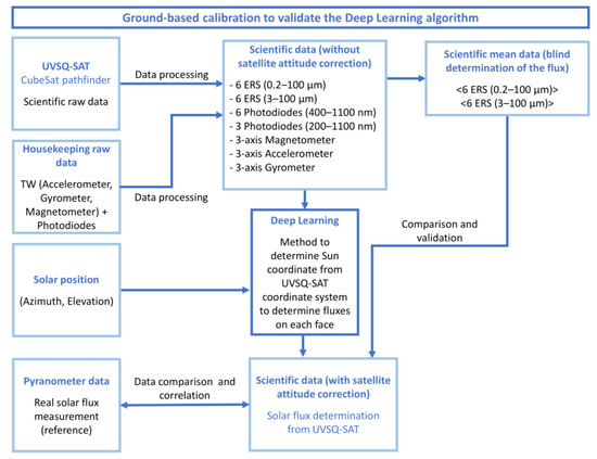
Figure 2.
Ground-based calibration implemented to train and validate the satellite attitude determination algorithm.
For this phase, the objective of the algorithm is to determine the azimuth of the Sun according to the satellite’s frame of reference at any time thanks to the measurements made by the satellite. We must train the algorithm as close as possible to in-orbit conditions. Therefore, managing to expose the satellite straight to the Sun with different orientations seemed to be the best option. The satellite was placed under a protection glass, on a mobile support, in an open area (Guyancourt, France). The support allowed us to modify the orientation of the satellite according to the position of the Sun. Since the final goal of the attitude determination is to measure the flux, we benefited from a reference instrument that performed flux measurement in parallel. This instrument was an SMP 6 model pyranometer from Kipp and Zonen, and was placed on another support which remained stationary throughout the experiment. The idea being to be able to compare the flux of the pyranometer to the flux measured by the satellite sensors corrected by its attitude.
The Satellite Inertial Measurements Unit (IMU) in the Teach’ Wear module contains a magnetometer, an accelerometer and a gyrometer. Therefore, knowing the Sun’s location at each time along with the information retrieved from the Satellite IMU, it is relatively practical to obtain the Sun’s position in the satellite’s frame of reference determining the rotational components as follows:
The satellite’s acceleration vector is defined as , represents the basis related to the satellite’s frame of reference, and is the basis related to the Teach’ Wear, inertial unit’s frame of reference, defined in Equations (1) and (2):
where represents the basis related to the satellite’s frame of reference, is the basis related to the Teach’ Wear, is the satellite’s acceleration vector, , , and are the three components of in and are measured by the accelerometer, , , and are the three components of the magnetic North in and are measured by the magnetometer, and , , forms the new basis.
The satellite’s reference frame is moving in the terrestrial reference frame, but the latter can be recovered using the Inertial Unit (IU) reference frame in Figure 3. The accelerometer recovers the gravity vector which defines one direction. The magnetometer retrieves the magnetic North, which, projected on the plane for which the normal is the gravity vector, defines another direction. The last direction is directly computed to create an orthonormal basis. This new basis is created from the intrinsic satellite basis and described in Equation (3):
where , , and are the three components of in , , , and are the three components of in , and , , and are the three components of in .
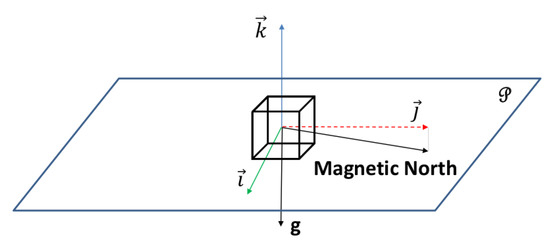
Figure 3.
Representation of the reference basis in the satellite frame of reference.
Therefore, it is straightforward to draw the rotation matrix related to each of those basis and consequently to find the angular position of the CubeSat during training in Equation (4):
The solar position is given thanks to reference data or algorithms and its azimuth and elevation can then be converted thanks to the previous rotation matrix so that they appear in the satellite frame of reference.
The output of the trained algorithm should be the relative azimuth previously computed; it corresponds to the azimuth of the Sun in the satellite’s frame of reference. In the training phase, the error between this output and the computed reference position will be quantified using a loss function. This function is detailed in Section 2.2.3. The output is then used to retrieve the solar flux and quantitatively validated thanks to the reference pyranometer.
As a summary, training/test/validation datasets are all the inputs (solar elevation in the satellite reference frame along with the normalized signals from the ERS sensors and the photodiodes) and reference outputs (cosine and sine of the solar azimuth in the satellite reference frame) of the UVSQ-SAT MLP neural network. We have chosen to randomly distribute these previous samples in the three different datasets so that about 70% of the samples will be in the training set, 15% in the validation set, and 15% in the test set.
The inputs are generated from the sensors. Outputs are generated from calculations. The azimuth was first generated in the terrestrial reference frame thanks to a NREL algorithm and was then transformed to the satellite reference frame, previously defined thanks to the on-board accelerometer and magnetometer.
2.2.2. Neural Network Architecture of the Deep Learning Method
The diagram in Figure 4 describes the neural network architecture implemented and how it is trained and validated during the experiments. The architecture is an MLP neural network, which is a computational model with 587 neurons. Multilayer Perceptrons are the classical type of neural network. They are suitable for regression prediction problems where a real-valued quantity is predicted given a set of inputs. The hyper-parameters (number of layers, learning rate, layer width, activation function, …) of the UVSQ-SAT MLP neural network were empirically determined based on output accuracies and rates of convergence of the loss function.
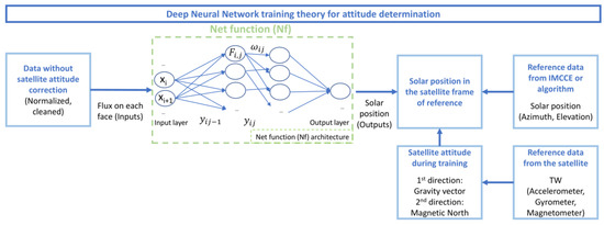
Figure 4.
Neural Network architecture with fully connected layers, as well as the inputs and outputs.
The inputs are detailed in the following explanation. It is here the ideal case, and for an optimum the output predicted should be the solar position that is computed following the procedure mentioned in Section 2.2.1.
For each layer represented in Figure 4, the functions that are applied to the inputs of the related layers structure the Net Function and are defined in Equations (5) and (6):
where are the outputs and are the inputs of the node (i,j), and , l is the total number of layers, is the cache output before going through the activation function, is the number of neurons at layer j, g is the activation function, are the weights, and are called the biases.
For the UVSQ-SAT’s training, due to its efficiency and the ability to get more accurate outputs in Table 1, we choose to use the rectified linear unit (ReLU) activation function defined in Equation (7):

Table 1.
Averaged results obtained for each activation function comparing their mean squared error between the predicted and desired azimuth as well as the number of iterations to reach the optimum.
For a reference case, we switch to different activation functions in order to empirically determine the best one in terms of mean-squared-error on the results desired. The other parameters were constants. The number of iterations of reference was fixed to be 300 maximum. A comparison is represented in Table 1 for two trainings (different Kaiming uniform initialization of the weights). The Sigmoid activation function allows for computing the relative azimuth with the worst accuracy as the convergence of the neural network is much slower and would entail a much higher computation time (approximately 10,000 iterations).
The exact architecture of the MLP neural network used for the determination of attitude is such that the algorithm combines:
- 5 Hidden fully connected layers
- 25 Inputs
- 2 Outputs
- Learning rate of , determined empirically
- Layers dimensions (width): 25/48/128/256/128/2
We compared the alternative structures in terms of accuracy and convergence rate. Other activation functions (ELU, Tanh, Sigmoid, Leaky RELU) or value of the learning rate (optimal for ) would worsen the performance of the MLP neural network. Reducing the number of layers in the MLP neural network would decrease the accuracy of the system but increasing the number of layers would leave the accuracy unchanged with a longer computation time.
The instruments of interest to locate the Sun in the satellite’s frame of reference are the six panel photodiodes focusing in the 400–1100 nm wavelength range and the six ERS sensors focusing on the 0.2–100 m wavelength range.
The function takes signals from the ERS sensors (thermopiles) and photodiodes (LED) as inputs and the orientation angle as output (Figure 4). The 25 inputs for the neural network are four ERS sensors with Carbon NanoTubes signals from the four lateral sides of the CubeSat, at three different following times, making 12 inputs, along with the four photodiodes’ signals from the four lateral sides at the same three different times. The last input is the elevation of the Sun at the spacecraft coordinates. The idea was not to consider the upper and lower faces of the CubeSat as to be able to generalize the trained function to new conditions. Specifically, we assumed that the bottom not considered for training would respond very differently in orbit. It is also known that this side never sees the Sun during the training phase, so its detection seems impossible. As the desired output is an angle, a straightforward way to avoid discontinuities is to use two trigonometric functions cosine and sine of the output angle as two desired outputs to then easily compute the related angle using atan2 function. Then, the orientation of the satellite in terms of cosine and sine in time will not have discontinuities and will be continuous. During the experiment, no abrupt change of orientation has taken place, as no abrupt changes will occur in orbit according to the sampling frequency chosen for the satellite’s measurements. The orientation at different following times is correlated. Therefore, taking different values of the signals before and, after the instant we consider, seems logical. It is the equivalent of a second-order central in finite differences’ components. One more input is the elevation of the Sun, even though the dynamics of this parameter during the experiment is very small compared to that of the other inputs, the elevation that will be known at this stage as an input can influence the output in this three-dimensional problem.
2.2.3. Loss Function for Training the Deep Learning Neural Network
The loss function, also called cost function, characterizes the error between the predicted output and the targeted value of reference. In our case, as the deviation increases, we will have continuously worse results derived from the output. Therefore, as the predicted output is getting further from the reference value, the quantified error should be higher. In particular, we would rather have a small but regular error rather than very large errors a little less frequently since this would completely affect the precision of the flux measurement. Common loss functions are being investigated in [17].
Therefore, two bilateral loss functions that can be clearly defined are: Mean Squared Error (MSE) and Mean Absolute Error (MAE), which are defined in Equations (8) and (9):
where are the targeted values, are the predicted values, and n is the total number of data points.
The MSE function will give more weight to the outliers than the MAE function that will be more robust to those. If anomalies should be detected and taken into account, MSE is the function to use, but, if outliers are present in the training set and not in the test set, MAE should be chosen. Therefore, the most suitable function in our case is the MSE.
2.2.4. Performance and Uncertainties
Learning is based on optimization of the net function as mentioned above to obtain the most accurate output, close to the reference data. The samples are split into three sets. It is important that those sets are totally decorrelated. The first one is the train set that is used to optimize the net function. Another one is the validation set that is used to check the performance of the algorithm at each iteration over the train set. This is important as it is a great indication to whether the function is able to generalize to other samples of data in the validation set. It is critical as the net function’s parameters chosen are based on the iteration that minimizes the loss for the validation set. The last dataset is the test set for which the performance of the net function is evaluated. Figure 5 shows the loss evaluated at each iteration during the training for both of the train and validation set. It is clear that, at first, both of the computed losses decrease with the number of iterations. However, at some point, the loss value for the validation set starts increasing. We have reached a point where the neural network is over-fitting the data from the train set and is unable to generalize to a new dataset. The net function retained is chosen at the iteration, where the validation set loss reaches a minimum to avoid this over-fitting situation.
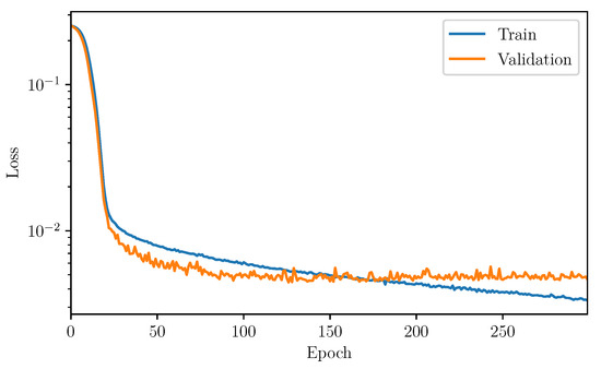
Figure 5.
Loss functions for the validation set and the train set at each iteration (Epoch) during training.
Here, the optimum for the validation set loss is reached at epoch 126 as the loss will increase after that epoch; this means that the algorithm is getting worse at generalizing to new samples. The performance of the function based on the last set is detailed in the following section.
3. Results
This section presents the results of the method to determine the UVSQ-SAT’s attitude using its housekeeping and scientific sensors’ measurements.
Section 2.2.2 presents the architecture chosen along with the hyper-parameters selected. The number of hidden layers, the learning rate, the activation function, the inputs, and the format of the outputs were meticulously studied and set for this issue. Those choices were made to optimize the deep learning algorithm for the training phase and the test phase. This architecture has been validated and constitutes a first result of our application to be replicated. To evaluate the ability of the algorithm to generalize to another set of samples, the net function optimized previously is applied to the test set with unseen data to compute the relative azimuth.
To validate the new method based on a deep learning approach to determine UVSQ-SAT in-orbit satellite attitude, a ground-based calibration experiment was carried out in October 2020 in Guyancourt (France), using the Sun as the radiative flux reference. In Figure 6, we compare the predicted azimuth of the Sun and the real ones that are used as a reference to assess the ability of this method to determine the on-ground orientation of the satellite. The root-mean-square deviation (RMSD) quantifies the error between the prediction and the real value. The first bisector is plotted as the ideal result from a perfect algorithm for which predicted azimuth would be equal to real azimuth characterizing the orientation of the CubeSat.
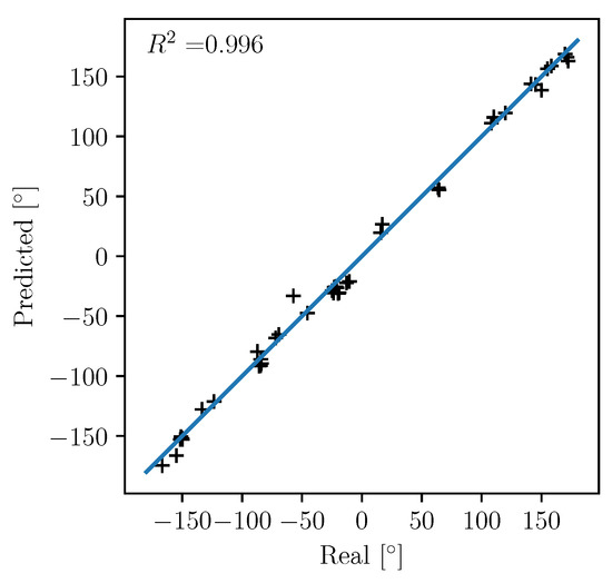
Figure 6.
Predicted azimuth of the Sun versus real azimuth of reference in degrees based on the test set done in October 2020 and the optimized neural network. The continuous blue curve represents the ideal case when the observed values perfectly fit the predicted values.
The correlation coefficient indicates a strong linear relationship between those angles which confirm the ability of the algorithm to learn and generalize. The root-mean-square deviation is evaluated at 7.1 at 1 using the previous function. It characterizes the error we would find on the precession angle of the satellite. Overall, the orientation itself is useful in that case to determine the nature of the flux observed at a given time and reconstruct the observed flux. In this case, we precisely know the actual configuration and we focus on the solar flux. In Figure 7, we evaluate the error induced on the calculation of the flux that is evaluated as a function of the recovered orientation. To do so, we present a comparison of the flux with correction of the attitude with the predicted azimuth, the real azimuth and the reference flux retrieved by the pyranometer. Then, to validate the method (MLP network to determine the attitude of orbiting satellites for spacecraft without active ADCS), measurements made by UVSQ-SAT instruments and corrected by the attitude of the satellite are compared with those measured by a pyranometer (independent measurements taken on the ground).
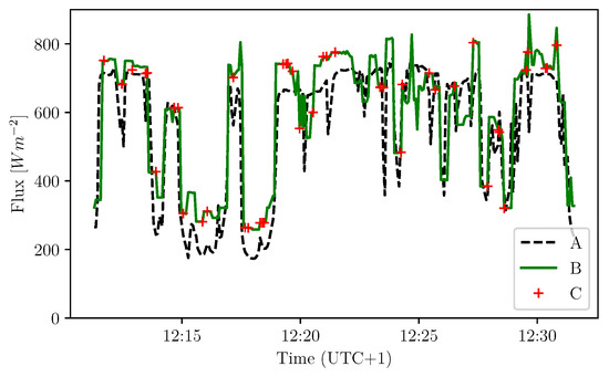
Figure 7.
Comparison of the different solar flux computations for the test conducted on 26 October 2020. (A) pyranometer flux corrected of the Sun’s elevation; (B) photodiodes’s flux corrected of the reference attitude; (C) photodiodes’s normalized flux corrected of the predicted attitude.
We want to measure the solar flux; this computation can only be applied here as conditions will differ in-orbit, but the main idea stays similar. As we retrieved the predicted attitude from the deep learning method with the accuracy mentioned above, we are able to determine which sides of the CubeSat are facing the Sun and which ones are not. In order to remove noise and reflections from the environment, we removed at each time the average ambient flux that is detected by the sides that are not directly facing the Sun. Then, we select the measurements from the sensors that are facing the Sun with a minimal angle of about 60 degrees (in a 120 degrees field of view). The measurements are then corrected using the dot product between the Sun’s direction and the normal vector relatively to each of the faces of the CubeSat facing the Sun (see Equations (10) and (11)). This parameter is directly linked to the attitude of the satellite recovered previously. By doing this, we discriminated the faces that were hidden from the Sun similarly to in-orbit conditions when sensors will face the Earth and would measure the albedo while others will directly measure incoming solar flux.
At each time of the experiment, we have:
where is the incoming solar flux, is the flux on face k of the satellite for the selected field of view, 0, otherwise, k is the index of the faces, is the the Sun position vector, is the normal vector to the face , is the dot product between and . The idea is to compute the average using the dot products as weights for the flux computed on each face facing the Sun such as:
The results obtained to compute the solar flux using the predicted attitude of the satellite are closer to the flux measured by the pyranometer than to blindly compute an average from the six different faces of the CubeSat. The configuration of the experiment requires good weather conditions. The ideal case is to have a sunny day without cloud. During the UVSQ-SAT ground-based calibration using the Sun as reference, the solar irradiance had to be at least 200 Wm. The solar irradiance measurement was carried out by a dedicated pyranometer (SMP 6 model from Kipp & Zonen) calibrated according to international standards. The SMP 6 measures solar irradiance on a planar surface, and it is designed to measure the solar radiation flux density (Wm) from the hemisphere in the 280 to 3000 nm spectral range. The directional response of the pyranometer has a deviation of less than 10 Wm from a direct beam of 1000 Wm up to a zenith angle of 80. Observing at the zenith, the deviation is negligible. For the UVSQ-SAT measurements, the flux of each sensor on each face of the satellite has been corrected of the attitude (direction of the line of sight of the Sun). The angular flux correction of each face of the satellite is based on Equation (10).
In Figure 7 and Figure 8, we compare the flux computed with predicted and reference orientation as well as the flux retrieved from the pyranometer. To quantify the error of our prediction, we compute the RMSD between the flux computed with the azimuth of reference and the flux computed thanks to the predicted azimuth. The RMSD of the residue of the ratio of the compared flux quantifies the normalized error between those fluxes. We find 0.1261 between the pyranometer flux and the predicted flux from the photodiodes. However, it appears that most of that error already exists between the reference flux and the pyranometer flux as the RMSD between those two fluxes, which is equal to 0.1255. First of all, we compute what we call the reference flux. It is defined by the solar flux that we would compute from the satellite’s photodiodes with Equation (11), if we would know the real orientation of the satellite at each time. This would happen if the algorithm would perfectly predict the satellite attitude at each time. For the pyranometer flux, we retrieve the data from the SMP 6 calibrated pyranometer. The instrument was located next to the satellite in order to get as close as possible to the observation conditions of the satellite. The pyranometer data are interpolated to suit the satellite time scale. We can then compare the different values found with the two different methods applying the root mean square deviation. For the photodiodes, we retrieve an RMSD of 0.0219 between the reference and predicted attitude corrected flux from the photodiodes. Here, we compared the previously computed reference flux and the flux obtained with the same computation method but considering predicted orientation instead of the real one. In the context of the experiment, one cannot claim to compare the two instruments in absolute terms, since the measurements are made under different conditions and having different instrument specifications. However, we can compare the flux obtained using the reference/targeted orientation of the CubeSat and the flux retrieved determining the attitude using the deep learning algorithm. The root-mean-square deviation between the flux corrected with the predicted attitude and the flux corrected with the known attitude is equal to 16 Wm or about 2 % in terms of RMSD of the residue.
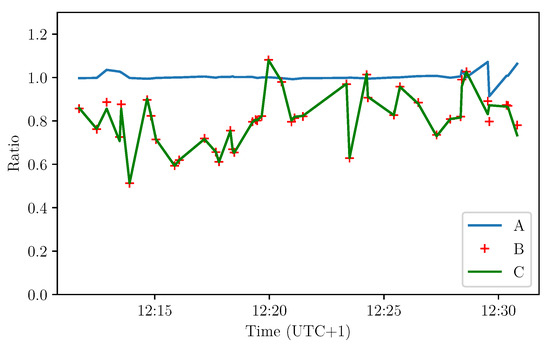
Figure 8.
Ratio of the flux for the pyranometer and the corrected flux thanks to the reference and predicted attitude. (A) ratio between the reference flux and the predicted flux; (B) ratio between pyranometer flux and the predicted flux; (C) ratio between the pyranometer flux and the reference flux.
4. Discussion and Perspectives
UVSQ-SAT is the first in a future satellite constellation, as a demonstrator to measure incoming and outgoing radiation at the TOA using miniaturized sensors on its six faces. To retrieve the required flux to compute the terrestrial net radiation, it is necessary to discriminate the flux measured from some of the sensors to select only solar flux or terrestrial radiation in the longwave or in the shortwave. It is also relevant to correct the different flux knowing the angle between the source of the flux and the instrument. To do so, the orientation of the satellite must be known at each time. However, small satellites such as UVSQ-SAT do not have an active ADCS, mainly due to limitations of mass, volume, and power. Therefore, another method using available sensors can be adopted to have a good knowledge of the satellite attitude. The UVSQ-SAT attitude determination algorithm using deep learning methods allowed for retrieving the orientation of the satellite on-ground thanks to its sensors on its sides. The algorithm was accurate at ±7.1 at 1. It helped select and measure the desired flux with an accuracy of 16 Wm.
However, there are several limitations that need to be taken into account for the next step and to apply the method to in-orbit attitude determination. As the amount of samples available to train the algorithm was not optimal during the ground test, the accuracy of the algorithm was limited due to over-fitting issues. Thousands of different samples including different orientations on the three-axis would have been better to train the neural network. During the experiment that aimed to retrieve signals to train the algorithm, the satellite was initially enclosed in a transparent box at ambient temperature and pressure. Therefore, temperature measurements on each side of the CubeSat could not be relevant for the study. Indeed, the convective heat transfer effects taking place during the experiment will be non-existent in-orbit. The responses of the temperature sensors will therefore be different in-orbit. The average temperature kept increasing with time as the enclosure got warmer and warmer. Thus, these are unusable for training on the ground. In orbit, using the temperature sensors will be really relevant and helpful for the determination of the attitude. It will improve the accuracy of the algorithm. Moreover, the UVSQ-SAT is equipped with three narrow field of view (NFOV) UVS sensors that will be pertinent for the Sun’s detection.
To take the differences between in-orbit and on-ground conditions into consideration, in-orbit training will be required to retrieve accurate predictions from the algorithm. The idea is to implement adaptation domains to benefit from the on-ground training and to adapt to targeted in-orbit responses. To retrieve the complete attitude of the satellite, we showed a way to compute the precession angle knowing the nutation and spin angles that define the plane characterized by its nadir normal vector. This plane was considered as a reference as the algorithm was trained on-ground but in-orbit; this will need to be implemented. Therefore, the first step of that method will be to train the neural network using an Attitude and Heading Reference System (AHRS) to determine the Earth’s position and therefore the previous plane.
Other main limitations of the ground calibration were the inefficiency of the ERS sensors (between 3 and 100 m) due to diffuse ambient temperature, and the fact that we could only search the Sun on a small excursion. This means that we were unable to rotate the satellite in the plane normal to Earth and slightly tilted it, but we could not flip the satellite upside down, and we therefore only trained it in one hemisphere. Furthermore, even if this ground study allowed for verifying the feasibility of our method, we only had one very bright source to find in the sky, while in flight we also have the Earth reflecting the Sun. This is why we are going to do a flight training in accordance with the method presented in Section 2 (and now demonstrated) and with the following solution, where one of the first steps will be to calibrate the magnetometer in-orbit.
Thanks to the Teach’ Wear magnetometer data, we know the three components of the magnetic field for each measurement, whose positions are calculated with the orbital parameters. Then, the International Geomagnetic Reference Field (IGRF-13) model gives the expected magnetic field, which allows for calibrating the UVSQ-SAT TW magnetometer. Then, a resulting map will be obtained and will illustrate the correct calibration of the system. While the mean of the field will be good, the instantaneous signal on each component will be noisy. This is why we will use a Kalman filter to reduce the noise such as explained in [18]. Since we will have the magnetic field vector in two reference frames, we will calculate the change of reference matrix in order to roughly orientate the satellite. We will then manually improve the accuracy of the attitude of the satellite by using the other sensors (photodiodes (LED), temperatures (solar cells), ERS sensors), in order to get data for learning steps. Some methods that will be implemented in-orbit can be described here. The objective to improve the algorithm is to determine the Earth’s location in the satellite’s frame of reference thanks to the ERS sensors (second type described in Section 2) measuring the radiation in the 3–100 m wavelengths range. We will compute the barycenter of the coordinates of the center of the faces assigned with the coefficients corresponding to those fluxes. The recovered vector will indicate the direction where the infrared flux is the highest, which means the Earth’s direction. A method that will be used in some orientations of the satellite to refine the detection of the Sun will be based on the use of the UVS sensors. They have a very narrow field of view allowing for having a better accuracy on the location of the Sun in the satellite’s reference frame. The orbital parameters and the National Renewable Energy Laboratory method described in [15] allow for retrieving the azimuth and the elevation of the Sun at each time based on the satellite’s location. Therefore, we will obtain the orientation of the satellite. This method will only be used to train the algorithm but cannot be always relevant in the case of eclipses. We will perform in-orbit training thanks to the previous computed output and the signals from the different sensors. First, measurements were recovered from the satellite since 24 January 2021. UVSQ-SAT solar cells temperature, photodiodes flux (LED), and the magnetic in-orbit variations are shown in Figure 9, Figure 10 and Figure 11. This temperature and flux are proof of the satellite’s good health and will be used as inputs for the neural network. The magnetic field will help us with the training phase as described previously. These inputs will be used to estimate the UVSQ-SAT attitude in orbit. This analysis will be the subject of another manuscript.
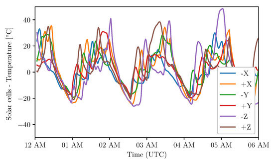
Figure 9.
Solar cells temperature for all UVSQ-SAT faces. Measurements start from 7 February 2021 at 12:00 AM (UTC). The orbital period is about 95.18 mn. UVSQ-SAT spins during the orbit.
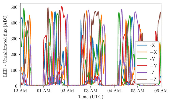
Figure 10.
Uncalibrated LED flux (photodiodes in the 400–1100 nm wavelength range) for all faces of the UVSQ-SAT CubeSat. Measurements (TSI + OSR) start from 7 February 2021 at 12:00 AM (UTC).
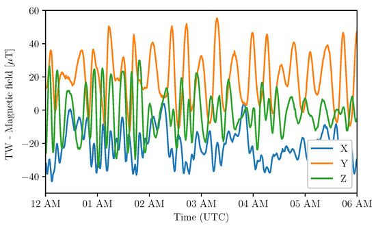
Figure 11.
Magnetic field components on the x-axis, y-axis, and z-axis.
5. Conclusions
The UVSQ-SAT space-based mission (technological demonstrator) aims to implement miniaturized and disruptive technologies for remote sensing with compact sensors. It is a first step towards a future satellite constellation mainly to measure the terrestrial net radiation. Terrestrial net radiation can be obtained with radiometers on all faces of the satellites that measure solar flux and fluxes of short-wave and long-wave radiation.
In this manuscript, we presented a new method based on a deep learning approach to retrieve terrestrial net radiation from satellites without attitude and orbital control system. Knowledge of the satellite attitude allows for applying the appropriate corrections to the incident flux measurements (solar (TSI), albedo (OSR), infrared (OLR)) on all faces of the spacecraft. Thus, the attitude determination is crucial for the computation of the fluxes. Therefore, we performed a ground-based calibration to validate and check the performance of the developed method that seems to be efficient. It was able to provide convenient results on the satellite attitude determination and its resulting fluxes.
We plan to improve its accuracy by increasing the number of training samples as well as by performing training under in-orbit conditions. More specific training will allow compliance with the mission specifications for measuring the EEI. This method represents a new way to determine the attitude of satellites and the terrestrial net radiation retrieval for the case of a constellation of small satellites.
UVSQ-SAT was successfully launched on 24 January 2021 into a Sun-synchronous orbit (at 535 km) thanks to a Falcon 9 rocket (Space X). During the commissioning phase, an in-orbit calibration will be done to consolidate the method described in this manuscript. The main goal will be to minimize the uncertainty on the knowledge of the UVSQ-SAT CubeSat attitude.
Based on the deep learning method applied to space-based attitude determination of the satellite with a great number of data samples, the uncertainty on the outgoing longwave radiation and shortwave radiation determination should be less than ±5 Wm (1).
Author Contributions
Conceptualization, A.F., M.M., C.D., T.B., S.B., A.H., P.K., A.S. and L.D.; methodology, A.F., C.D., M.M. and T.B.; software, A.F.; validation, A.F.; formal analysis, A.F.; investigation, M.M.; resources, M.M.; data curation, A.F.; writing—original draft preparation, A.F.; writing—review and editing, A.F., C.D., M.M., T.B. and A.M.; visualization, C.D.; supervision, M.M.; project administration, M.M.; funding acquisition, M.M. All authors have read and agreed to the published version of the manuscript.
Funding
The UVSQ-SAT research was mainly funded by Centre National de la Recherche Scientifique (CNRS, France), Centre National d’Études Spatiales (CNES, France), UVSQ (Université de Versailles Saint-Quentin-en-Yvelines, France), and Agence Nationale de La Recherche (ANR, France). This work was supported by the Programme National Soleil Terre (PNST) of CNRS/INSU (France) co-funded by CNES and Commissariat à l’énergie atomique (CEA, France).
Acknowledgments
The authors acknowledge support from the Centre National de la Recherche Scientifique (CNRS, France), the Centre National d’Études Spatiales (CNES, France), and Office National d’Études et de Recherches Aérospatiales (ONERA, France). The authors would like to thank the reviewers for their assistance in evaluating this manuscript.
Conflicts of Interest
The authors declare no conflict of interest.
References
- Meftah, M.; Damé, L.; Keckhut, P.; Bekki, S.; Sarkissian, A.; Hauchecorne, A.; Bertran, E.; Carta, J.P.; Rogers, D.; Abbaki, S.; et al. UVSQ-SAT, a pathfinder cubesat mission for observing essential climate variables. Remote Sens. 2020, 12, 92. [Google Scholar] [CrossRef]
- Meftah, M.; Damé, L.; Bolsée, D.; Hauchecorne, A.; Pereira, N.; Sluse, D.; Cessateur, G.; Irbah, A.; Bureau, J.; Weber, M.; et al. SOLAR-ISS: A new reference spectrum based on SOLAR/SOLSPEC observations. Astron. Astrophys. 2018, 611, A1. [Google Scholar] [CrossRef]
- Meftah, M.; Snow, M.; Damé, L.; Bolseé, D.; Pereira, N.; Cessateur, G.; Bekki, S.; Keckhut, P.; Sarkissian, A.; Hauchecorne, A. SOLAR-v: A new solar spectral irradiance dataset based on SOLAR/SOLSPEC observations during solar cycle 24. Astron. Astrophys. 2021, 2, 1–9. [Google Scholar] [CrossRef]
- Stephens, G.L.; Li, J.; Wild, M.; Clayson, C.A.; Loeb, N.; Kato, S.; L’Ecuyer, T.; Stackhouse, P.W.; Lebsock, M.; Andrews, T. An update on Earth’s energy balance in light of the latest global observations. Nat. Geosci. 2012, 5, 691–696. [Google Scholar] [CrossRef]
- Allan, R.P.; Liu, C.; Loeb, N.G.; Palmer, M.D.; Roberts, M.; Smith, D.; Vidale, P.L. Changes in global net radiative imbalance 1985–2012. Geophys. Res. Lett. 2014, 41, 5588–5597. [Google Scholar] [CrossRef] [PubMed]
- Wild, M.; Ohmura, A.; Schär, C.; Müller, G.; Folini, D.; Schwarz, M.; Hakuba, M.Z.; Sanchez-Lorenzo, A. The Global Energy Balance Archive (GEBA) version 2017: A database for worldwide measured surface energy fluxes. Earth Syst. Sci. Data 2017, 9, 601–613. [Google Scholar] [CrossRef]
- Brasoveanu, D.; Hashmall, J.; Baker, D. Spacecraft Attitude Determination Accuracy from Mission Experience. NASA GSFC Tech. Rep. 1994, 95, 12858. [Google Scholar]
- Markley, F.L.; Crassidis, J.L. Static Attitude Determination Methods. In Fundamentals of Spacecraft Attitude Determination and Control; Springer: New York, NY, USA, 2014; pp. 183–233. [Google Scholar] [CrossRef]
- Iwasaki, Y.; Kikuya, Y.; Sasaki, K.; Ozawa, T.; Shintani, Y.; Masuda, Y.; Watanabe, K.; Mamiya, H.; Ando, H.; Nakashima, T.; et al. Development and Initial On-orbit Performance of Multi-Functional Attitude Sensor using Image Recognition. In Proceedings of the AIAA/USU Conference on Small Satellites, Logan, UT, USA, 3–8 August 2019. [Google Scholar]
- Zhu, X.X.; Tuia, D.; Mou, L.; Xia, G.; Zhang, L.; Xu, F.; Fraundorfer, F. Deep Learning in Remote Sensing: A Comprehensive Review and List of Resources. IEEE Geosci. Remote Sens. Mag. 2017, 5, 8–36. [Google Scholar] [CrossRef]
- Malerba, M.E.; Wright, N.; Macreadie, P.I. A continental-scale assessment of density, size, distribution and historical trends of farm dams using deep learning convolutional neural networks. Remote Sens. 2021, 13, 319. [Google Scholar] [CrossRef]
- Debella-Gilo, M.; Gjertsen, A.K. Mapping Seasonal Agricultural Land Use Types Using Deep Learning on Sentinel-2 Image Time Series. Remote Sens. 2021, 13, 289. [Google Scholar] [CrossRef]
- Rostami, M.; Kolouri, S.; Eaton, E.; Kim, K. Deep transfer learning for few-shot SAR image classification. Remote Sens. 2019, 11, 1374. [Google Scholar] [CrossRef]
- Shao, Z.; Zhou, Z.; Huang, X.; Zhang, Y. Mrenet: Simultaneous extraction of road surface and road centerline in complex urban scenes from very high-resolution images. Remote Sens. 2021, 13, 239. [Google Scholar] [CrossRef]
- Reda, I.; Nrel, A.A. Solar Position Algorithm for Solar Radiation Applications (Revised); National Renewable Energy Laboratory Nrel/Tp-560-34302; National Renewable Energy Laboratory: Golden, CO, USA, 2005; pp. 1–56. [Google Scholar]
- Finance, A.; Meftah, M.; Mangin, A.; Keckhut, P. UVSQ-SAT a New Way to Obtain Spatio-Temporal Variations of the Radiation Budget with a Satellite Constellation; Earth and Space Science Open Archive; American Geophysical Union: Washington, DC, USA, 2021; p. 21. [Google Scholar] [CrossRef]
- Nie, F.; Hu, Z.; Li, X. An investigation for loss functions widely used in machine learning. Commun. Inf. Syst. 2018, 18, 37–52. [Google Scholar] [CrossRef]
- Martel, F.; Pal, P.K.; Psiaki, M.L. Three-axis attitude determination via Kalman filtering of magnetometer data. J. Guid. Control. Dyn. 1990, 13, 344–367. [Google Scholar]


Publisher’s Note: MDPI stays neutral with regard to jurisdictional claims in published maps and institutional affiliations. |
© 2021 by the authors. Licensee MDPI, Basel, Switzerland. This article is an open access article distributed under the terms and conditions of the Creative Commons Attribution (CC BY) license (http://creativecommons.org/licenses/by/4.0/).