Article

Spring Frost Damage to Tea Plants Can Be Identified with Daily Minimum Air Temperatures Estimated by MODIS Land Surface Temperature Products

1
State Key Laboratory of Severe Weather, Chinese Academy of Meteorological Sciences, Beijing 100081, China
2
Fujian Institute of Meteorological Science, Fuzhou 350001, China
3
Zhejiang Climate Center, Hangzhou 310017, China
4
Collaborative Innovation Center of Meteorological Disaster Forecast, Early-Warning and Assessment, Nanjing University of Information Science & Technology, Nanjing 210044, China
*
Author to whom correspondence should be addressed.
Remote Sens. 2021, 13(6), 1177; https://doi.org/10.3390/rs13061177
Submission received: 1 February 2021 / Revised: 7 March 2021 / Accepted: 14 March 2021 / Published: 19 March 2021
(This article belongs to the Special Issue Remote Sensing for Agrometeorology)

Abstract

:
Tea (Camellia sinensis) is one of the most dominant economic plants in China and plays an important role in agricultural economic benefits. Spring tea is the most popular drink due to Chinese drinking habits. Although the global temperature is generally warming, spring frost damage (SFD) to tea plants still occurs from time to time, and severely restricts the production and quality of spring tea. Therefore, monitoring and evaluating the impact of SFD to tea plants in a timely and precise manner is a significant and urgent task for scientists and tea producers in China. The region designated as the Middle and Lower Reaches of the Yangtze River (MLRYR) in China is a major tea plantation area producing small tea leaves and low shrubs. This region was selected to study SFD to tea plants using meteorological observations and remotely sensed products. Comparative analysis between minimum air temperature (Tmin) and two MODIS nighttime land surface temperature (LST) products at six pixel-window scales was used to determine the best suitable product and spatial scale. Results showed that the LST nighttime product derived from MYD11A1 data at the 3 × 3 pixel window resolution was the best proxy for daily minimum air temperature. A Tmin estimation model was established using this dataset and digital elevation model (DEM) data, employing the standard lapse rate of air temperature with elevation. Model validation with 145,210 ground-based Tmin observations showed that the accuracy of estimated Tmin was acceptable with a relatively high coefficient of determination (R2 = 0.841), low root mean square error (RMSE = 2.15 °C) and mean absolute error (MAE = 1.66 °C), and reasonable normalized RMSE (NRMSE = 25.4%) and Nash–Sutcliffe model efficiency (EF = 0.12), with significantly improved consistency of LST and Tmin estimation. Based on the Tmin estimation model, three major cooling episodes recorded in the "Yearbook of Meteorological Disasters in China" in spring 2006 were accurately identified, and several highlighted regions in the first two cooling episodes were also precisely captured. This study confirmed that estimating Tmin based on MYD11A1 nighttime products and DEM is a useful method for monitoring and evaluating SFD to tea plants in the MLRYR. Furthermore, this method precisely identified the spatial characteristics and distribution of SFD and will therefore be helpful for taking effective preventative measures to mitigate the economic losses resulting from frost damage.

Graphical Abstract

1. Introduction

Tea plant (Camellia sinensis) is a species of evergreen shrubs or small trees in the flowering plant family Theaceae whose leaves and leaf buds are used to produce tea drink. Tea, along with coffee (Coffea arabica L.) and cocoa (Theobroma cacao L.), has been used to make most of the traditional and popular caffeinated beverages [1] in the world. Differences in tea taste are determined by the degree of fermentation. There are seven classifications of tea, including black tea, white tea, yellow tea, green tea, oolong tea, dark tea, and reprocessing tea, based on how they are processed and how long the leaves are left on the shrub before harvesting [2].
Tea plant originated in southeast China and was gradually introduced into many tropical and subtropical countries [3]. At present, more than 60 countries and regions around the world plant tea trees, mainly distributed in tropical and subtropical climate areas between 16°S and 30°N [4]. Some varieties also grow well in cooler climates and high altitude regions, such as the mild climate of the U.S. Pacific Northwest and the Yunnan–Guizhou Plateau of southwestern China. The worldwide harvested tea area reached 3.56 × 10⁶ ha in 2018 with a production of 5.11 × 10⁹ kg [5]. Of all of the countries of the world, China harvested the greatest area (66.0% of the world total) and produced the greatest amount (51.4% of the world total) of tea, followed by India. These two countries accounted for 83.7% of the world tea harvested area and 77.8% of the world tea production [5]. The 18 provinces in China where planting of tea plants is concentrated are located in North China, Central China, South China, and Southwest China.
Tea can be divided into four categories according to the harvest season: spring tea, summer tea, autumn tea, and winter tea. Spring tea is usually harvested from March to the middle of May. Compared with teas harvested in other seasons, the spring leaves are softer, the buds are plumper, the color is greener, the vitamins and amino acids are richer, and the flavor tastes more refreshing due to moderate temperatures and higher relative air humidity in spring [6,7]. Therefore, spring tea is an important segment of the tea market because of its high quality and the highest economic benefits for tea production all over the world. For example, the economic benefits of spring tea accounted for 87.5% of the total tea revenue in 2019 in Zhejiang Province in China [8].
According to climate model projections, the global average air temperature is likely to increase by 0.3–4.8 °C by the end of this century [9]. However, research in recent years has also revealed that the frequency, intensity, and duration of extreme low temperature events are also likely to continuously increase under 21st-century warming scenarios [10,11]. Additionally, the predicted spring frost risk correspondingly increases under future climate warming [12].
Frost damage can be divided into advection frost and radiation frost according to its formation mechanism [13]. An advection frost occurs when cold air blows into an area to replace warmer air that was present before the weather change. It is associated with moderate to strong winds and low humidity [13]. Radiation frosts occur because of heat losses in the form of radiant energy. Under clear nighttime skies, the soil surface loses more longwave radiation (heat) to the atmosphere than it receives [14], resulting in declining temperature. Radiation frosts are characterized by clear skies, calm winds, and temperature inversions [13]. During a radiation frost event, the ground and ambient air temperatures drop, and vegetation canopies experience temperatures that are 2–4 °C colder than the air temperature that is measured within a nearby standard Stevenson Screen thermometer enclosure. Spring frost is a catastrophic weather event that may cover a broad spatial region and is harmful to crops (winter wheat [15], winter sugar beet [16], potato [17]); orchards (apple [18], cherry [18], tea [19]); and forests (beech [20,21,22]), spruce [18]).
Different methods of spring frost identification and quantification have been studied in recent years, and generally fall into two categories: one is the spring frost index based on air temperature (Ta) measured with sensors inside meteorological station shelters at a height of 2 m above the ground surface, and the other is spring frost identification based on the land surface temperature (LST) derived from satellite remote sensing imagery. Ground-based meteorological observations showed that when daily minimum air temperature is less than 4 °C in spring, newly formed tea buds were impacted by spring frost [23], and the commodity value of the tea declined correspondingly. Therefore, tea leaf damage grades have been quantified based on daily minimum air temperature and its duration [24]. Li et al. [25] and Jin et al. [26] further refined this frost damage indicator by using hourly temperature and its duration. Meteorological data generally has high accuracy, high temporal resolution, and long-term observation datasets, and has therefore been used in many applications with regards to spring frost, such as identifying spatiotemporal distribution characteristics [27], and assessing impact [28] and risk [29]. Nevertheless, observation of Ta is limited by weather station network layout, resulting in point samples that often cannot effectively reflect spatial variation, especially in certain areas where the distribution of meteorological stations is itself very sparse [30], and in areas where elevation changes drastically.
Satellite remote sensing provides unprecedented global coverage of critical land surface parameters such as LST and vegetation indices. The Moderate Resolution Imaging Spectroradiometer (MODIS) onboard the Aqua and Terra satellites can provide such detailed information of land surface temperature at high temporal (daily or four times a day) and spatial (1 km or 250 m) resolution across the world [31]. Therefore, estimating Ta from LST has been a popular method because of the availability of LST products for regions with inadequate or inaccessible weather station networks [32]. Because solar radiation does not affect the thermal infrared signal during nighttime [31], the retrieval of minimum Ta (Tmin) from Aqua nighttime LST has been shown to be an effective method with a good relationship between nighttime LST and Tmin over different ecosystems in Africa [31,33], the U.S. Corn Belt [34], and xerophytic vegetation areas [29] and alpine meadows [35] on the northern Tibetan Plateau in Asia.
Despite recent progress in the use of satellite imagery, major limitations caused by cloud contamination remain [36] because LST products are unavailable when clouds exist during satellite overpassing times. Cloud contamination, therefore, has strong impacts on the availability and the quality of LST products [37]. Methods regarding LST reconstruction for cloudy regions, including the Harmonic Analysis of Time Series (HANTS) algorithm [38], Remotely Sensed DAily land Surface Temperature reconstruction (RSDAST) model [39], Bayesian Maximum Entropy (BME) method [40], and Random Forest (RF) regression approach [41], have been investigated by considering neighboring pixels and nearby dates based on normalized difference vegetation index, enhanced vegetation index, normalized difference water index, solar radiation factor, albedo, elevation, slope, longitude, and latitude. Results showed that all methods for reconstructing LSTs for cloud-covered regions were highly accurate compared with original LST pixels and produced spatial and temporal patterns of LST that were consistent with neighboring clear-sky areas [39,41]. Nevertheless, deviations between nighttime LST and Tmin values still exist due to the difference between satellite overpass time when LST is obtained and sunrise (generally the time of Tmin).
The main objective of this study was to study spring frost damage (SFD) to tea plants over the MLRYR in China at high temporal (daily) and spatial (1 km) resolutions. To reach this goal, we firstly introduced the study area and data in Section 2. Secondly, a simple regression model to estimate daily Tmin from reconstructed MODIS LST values was established by considering the terrain effects in methodology section. Next, values of MODIS nighttime reconstructed LST and Tmin were compared, and the performance of the regression model was evaluated in Section 4.1, Section 4.2 and Section 4.3. Then, several typical frost damage periods were identified and analyzed by using daily Tmin at the high-spatial resolution produced by the simple regression model. Additionally, the spatial distribution of different SFD levels for tea plants were mapped at 1 km resolution for selected typical SFD periods over the MLRYR in China (Section 4.4). Finally, some limitations were discussed, and the conclusion was summarized at the end of this paper.

2. Study Area and Data

2.1. Study Area

The MLRYR is located from 24° to 35°N latitude and from 109° to 122°E longitude. It covers six provinces (Jiangsu, Zhejiang, Anhui, Jiangxi, Hubei, and Hunan) and Shanghai municipality, with a total area of 1.01 × 10⁶ km2, accounting for 10.48% of China’s total land area (Figure 1). The climate of MLRYR is affected by the difference in thermal properties between land and sea and is therefore under the influence of a subtropical monsoon climate with hot and rainy summers, and cool and dry winters. The average annual temperature is 14–20 °C, and the annual precipitation is about 1000–1400 mm [42]. The seasonal distribution of precipitation is relatively even, but summer droughts occur occasionally.
The terrain of the MLRYR is relatively low and flat, with an elevation being below 50 m above sea level in most areas. The low mountains and hills scattered in the west and south, and the elevations were between 200 and 1000 m (Figure 1b). The vegetation coverage is high in the MLRYR, and includes forest, grass, crop, and shrub (Figure 1c). The tea plants are one of the majority types of shrubs, which distributed mainly in low mountains and hills with the elevation being below 1000 m.

2.2. Data

2.2.1. Meteorological Data

Daily Tmin at 163 meteorological stations from March to April in 2003–2018 in the MLRYR were obtained from ground meteorological stations (available at http://data.cma.cn/site/index.html. Last visited on 17 March 2021) and measured in line with World Meteorological Organization (WMO) standards at 2 m above the ground (Figure 1). All data were quality checked, and there were not any missing temperature records in this study area.

2.2.2. MODIS Products

(1)
MODIS LST products
Because of the good relationship between MODIS nighttime LST and Tmin values reported in previous research, daily MODIS nighttime LST products (MOD11A1 and MYD11A1) on board the Terra and Aqua satellites (version 6) at 1 km spatial resolution in a 1200 by 1200 km grid were downloaded via the Earth Observing System Data and Information System (EOSDIS) of the National Aeronautics and Space Administration (NASA) (https://earthdata.nasa.gov/. Last visited on 17 March 2021). The orbit of Terra around the Earth passes from north to south at about 10:30 a.m. and p.m. local solar time, while Aqua passes in the opposite direction from south to north at about 1:30 p.m. and a.m. every day. MODIS LST products are retrieved from the MODIS thermal and middle infrared spectral regions using the generalized split window algorithm [43] that corrects for atmospheric effects. The LST products of four tiles (h27v05, h28v05, h27v06, and h28v06) from 2003 to 2018 were re-projected to Albers Conical Equal Area (ACEA) projection, and then merged, resized, and mosaicked to get the dataset that was exactly consistent with the study area on each day during the study period.
(2)
MODIS Land Cover Type products
The MODIS Land Cover Type product (MCD12Q1) supplies global maps of land cover at annual time steps and 500 m spatial resolution for 2001–present [44]. The product contains five legacy classification schemes, including IGBP (International Geosphere-Biosphere Programme), UMD (University of Maryland), LAI (Leaf Area Index), BGC (BIOME-Biogeochemical Cycles), and PFT (Plant Functional Types). PFTs reduce the complexity of species diversity in ecological function to a few key plant types. Shrub, defined as a woody plant with more than 10% coverage rate and 1–2 m height, was extracted to identify the tea planting area in the MLRYR (Figure 1).

2.2.3. Digital Elevation Data

Digital elevation data were obtained from the Advanced Spaceborne Thermal Emission and Reflection Radiometer (ASTER) global digital elevation model V3 [45]. Digital elevation data with 30 m spatial resolution was stored in a raster file. To aggregate up to the MODIS LST resolution, the mean elevation value inside each of the 1-km grid cells was calculated. Meanwhile, elevation values within 3 × 3, 5 × 5, 7 × 7, 9 × 9, and 11 × 11 grid cells at 1-km resolution were aggregated up to get six DEM images at the 3-km, 5-km, 7-km, 9-km, and 11-km resolutions, respectively.

2.2.4. Historical Disaster Records

Historical spring frost disaster records for tea plants were acquired from the "Yearbook of Meteorological Disasters in China" (from 2004 to 2017). The records described the onset date, duration, and location of spring frost events. For example, the "Yearbook of Meteorological Disasters in China" (2007) [46] recorded the following: “From March 11 to 13, Jiangxi province generally experienced a strong cold wave weather process with strong winds, cooling, and snowfall as the main characteristics in 2006. The affected area of crops was 119,000 hectares, and the direct economic loss in agriculture was RMB 100 million. From March 27 to 28, the maximum temperature dropped in most parts of Jiangsu Province, and the maximum dropping range reached about 10 °C in 2006. On 12 April 2006, affected by the cold air moving eastward from the north to the south, the temperature in most parts of Jiangsu Province dropped by 8–11 °C within 48 h.”

3. Methodology

3.1. Reconstruction for MODIS LST

A clear sky MODIS LST reconstruction method (RSDAST) [39], was used in this study. RSDAST was developed based on the assumption that differences in LST between nearby pixels are relatively stable during a short time period [39]. Unlike other temperature reconstruction methods, RSDAST requires only one parameter (the MODIS LST product itself). Reconstructed LST values have shown accuracy in flat areas with the coefficient of determination (R2) of 0.72–0.89, bias of −0.02–0.21 K, and root mean square error (RMSE) of 0.92–1.16 K, while in complicated terrain regions of mountain areas, with an elevation range from 50 to 5000 m [39], the statistical values were R2 of 0.81–0.89, bias of −0.35 to −1.52 K, and RMSE of 1.42–2.24 K in Northwest China. The terrain of this study area is not so complicated, and includes plains, hills, and mountain regions, with an elevation range from 0 to 3000 m. Therefore, RSDAST was suitable for this study area to reconstruct gap-filled MODIS LST pixels.

3.2. Comparison between MODIS LST and Tmin at Meteorological Stations

Daily MODIS nighttime reconstructed LST values (MOD11A1_night and MYD11A1_night) were compared with daily Tmin observations at ground meteorological stations from 2003 to 2018. In order to make the comparison, MOD11A1_night and MYD11A1_night reconstructed values were first extracted for the pixels in which the ground meteorological stations were located. Additionally, the values of MOD11A1_night and MYD11A1_night reconstructed LST in 3 × 3, 5 × 5, 7 × 7, 9 × 9, and 11 × 11 pixel-windows centered on each meteorological pixel point were extracted, and the average LST values were calculated. The correlations between MODIS reconstructed LST values at each of the six window-scales and the Tmin values were compared by analyzing the bivariate correlations. Three statistical parameters, including R2, RMSE, and mean absolute error (MAE), were determined between Tmin and average reconstructed LST values for two MODIS nighttime products and six window scales. The most suitable MODIS LST product and window scale were selected by choosing the ones that produced the maximum R2 and minimum MAE and RMSE.

3.3. Estimation and Validation of Tmin

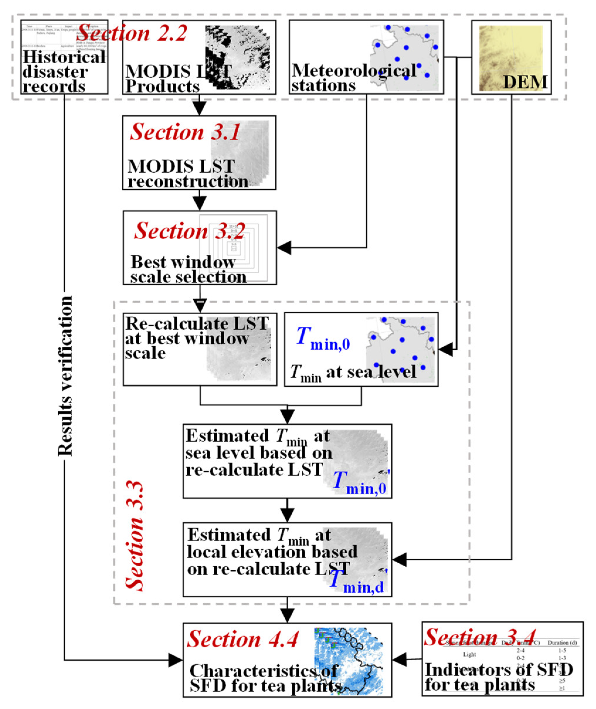
In the first layer of the atmosphere (the troposphere, approximately from sea level to 12 km upward), air temperatures drop steadily by an average of 6.5 degrees Celsius per one thousand meters (https://sciencing.com/info-8179549-happens-temperature-altitude-increases.html. Updated on 31 May 2019. Last visited on 31 August 2020) (the adiabatic lapse rate). Therefore, a Tmin estimation model based on MODIS LST and DEM was established according to the following three processes: (i) Tmin at the local elevation was first converted to sea level temperature using the standard lapse rate for air temperature; (ii) the regression model of Tmin at sea level was then built according to the average MODIS LST within the best window scale; (iii) finally, the Tmin at the local elevation was re-calculated based again on the standard lapse rate of air temperature. The specific expressions were as follows, and the pipeline and Tmin estimation method were also shown in Figure 2:
T m i n , 0 = T m i n , d 6.5 × D E M 1000
T m i n , 0 = a × L S T + b
T m i n , d = T m i n , 0 + 6.5 × D E M 1000
where T m i n , d and T m i n , d are the observed and estimated minimum air temperatures (°C) at local elevation, respectively; T m i n , 0 and T m i n , 0 are converted and regressed minimum air temperature (°C) at sea level, respectively; DEM is the digital elevation (m) averaged to the best window scale; LST is the average MODIS LST (°C) within the best window scale; a and b are the regression coefficients that are determined by fitting a least squares regression.
The estimated Tmin based on the average reconstructed LST values at the best pixel-window scale in this study was validated with Tmin observations at ground meteorological stations. Three statistics, including R2, MAE, and RMSE were computed to evaluate the method used for estimating Tmin. Additionally, the normalized RMSE (NRMSE) and the Nash–Sutcliffe model efficiency (EF) were also used to indicate how well the simulated values were consistent with the observed data. The simulation is considered excellent with NRMSE < 10%, good if 10–20%, acceptable if 20–30%, and poor > 30% [47]. Meanwhile, EF = 1, corresponds to a perfect match of the model to the observed data. EF = 0, indicates that the model estimations are as accurate as the mean of the observed data. If the EF is negative, it denotes that the observed mean is better than the model estimation [48,49].

3.4. Indicators of SFD for Tea Plants

Agrometeorological disaster indicators are the basis of damage studies for identifying the onset time, monitoring the spatial scope, predicting the extent, and evaluating the impacts of disasters [50,51]. These indicators vary with disaster types and crop varieties.
Low temperature is the prevailing factor affecting the degree of spring frost, but it is not the sole factor. Frost damage is also the result of continuous accumulation of low temperature [52]. Therefore, the combination of low temperature intensity and duration is an effective way to determine the impacts of frost damage on crop growth [53]. Based on the daily Tmin values and their duration, previous research has divided SFD of tea plants into three levels (light, moderate, and severe, Table 1) [54]. The indicators were effectively used to analyze the spatiotemporal distribution of SFD for Tea plants in southern Zhejiang [55] and its climatic characteristics in Zhejiang province in China [56]. Furthermore, Meng et al. took the spring frost process happened on 1 April 2019 as an example to evaluate the impacts of SFD on tea plants in Zhejiang province. The risk of SFD to tea plants was assessed temporally and spatially based on the SFD indicators and ground-based meteorological observations [57].

4. Results

4.1. Selection of the Best Window Scale for MODIS LST

Comparison results between Tmin and average reconstructed LST values for each nighttime product and window scale showed that MYD11A1 products were better than MOD11A1 with higher R2 and lower RMSE and MAE. Furthermore, as pixel-window numbers increased, the R2 between Tmin and reconstructed LST values exhibited the characteristics of a slightly increase first and then decrease for MYD11A1 products (Figure 3). The best correlation occurred when the window scale was 3 × 3. Previous research showed that a MODIS objective geolocation accuracy of 150 m at nadir view, and its geolocation errors were even larger at an off-nadir view [58]. Therefore, there may be some geolocation offset at the central pixel for each meteorological station. Additionally, some heterogeneous land surface with sharpening temperature in a larger window scale (such as 9 × 9 and 11 × 11) may also exist. These two situations can cause relatively lower correlations between Tmin and average reconstructed LST values at the corresponding window scale.
The RMSE and MAE values computed for both MOD11A1 and MYD11A1 increased linearly with increasing pixel-window scales (Figure 3). The minimum MAE occurred at the 1 × 1 and 3 × 3 window scales for the two MODIS nighttime LST products. When comparing the two MODIS nighttime LST products, MYD11A1 obtained from the Aqua satellite was much better than MOD11A1 obtained from the Terra satellite. The values of R2 were 0.7819 for MYD11A1 and 0.5961 for MOD11A1 for the 1 × 1 window size (Figure 3). The reasons for this difference may be related to the differences in satellite overpass times [30]. As mentioned previously, during the nighttime, the overpass times of Terra and Aqua are 10:30 pm and 1:30 am, respectively. In fact, daily minimum air temperature generally occurs around sunrise. Therefore, the LST nighttime values from MOD11A1 and MYD11A1 are higher than the minimum air temperatures observed at local meteorological stations, and LST derived from MOD11A1 is higher than from MYD11A1 because of the difference in overpass times of the two satellites. As a result, the LST nighttime product derived from MYD11A1 and the 3 × 3 pixel window is a better proxy for daily minimum air temperature. This result is consistent with previous research [59].

4.2. Characteristics of Temperature from March to April

4.2.1. Annual Dynamics of Daily Tmin and LST

Temporal dynamics of daily Tmin and reconstructed MYD11A1 nighttime LST at 3 × 3 window scale over all stations in the MLRYR from March to April in 2003–2018 are shown in Figure 4. Generally, both LST and Tmin exhibited a fluctuating increasing trend within each year. Temperatures were generally lower in early March and higher in late April. Similar to the results of other studies, Tmin was higher than MODIS LST [30] with a negative bias of −2.6 °C. The reasons for this difference are likely related to the intensity of solar radiation. Solar radiation heated the ground surface in spring is not very obvious due to the large soil heat capacity and low temperature accumulation.

4.2.2. Daily Dynamics of Average Tmin and LST

In order to further investigate the relationship of MYD11A1 nighttime reconstructed LST values to daily minimum air temperature, the daily Tmin and LST were averaged over all stations from March to April in 2003–2018. The time series curves of daily MYD11A1 nighttime reconstructed LST values and minimum air temperature are shown in Figure 5. Affected by long-term cloudy contamination, such as more than eight days [39], some LST values were not still able to be effectively reconstructed. Therefore, daily calculated sample numbers of LST values are different and they were also shown in the form of a histogram in Figure 5. Tmin and LST averaged over more than 2000 samples generally increased with time, and Tmin values were higher than LST values. The average difference between Tmin and LST was 2.56 °C, with maximum and minimum differences of 4.39 °C and 1.19 °C, respectively. Although temperature mostly increased with time from March to April, cooling periods sometimes occurred. The majority of these cooling periods appear to occur in mid-to-late March and early April, and therefore will have an important impact on tea plant production.

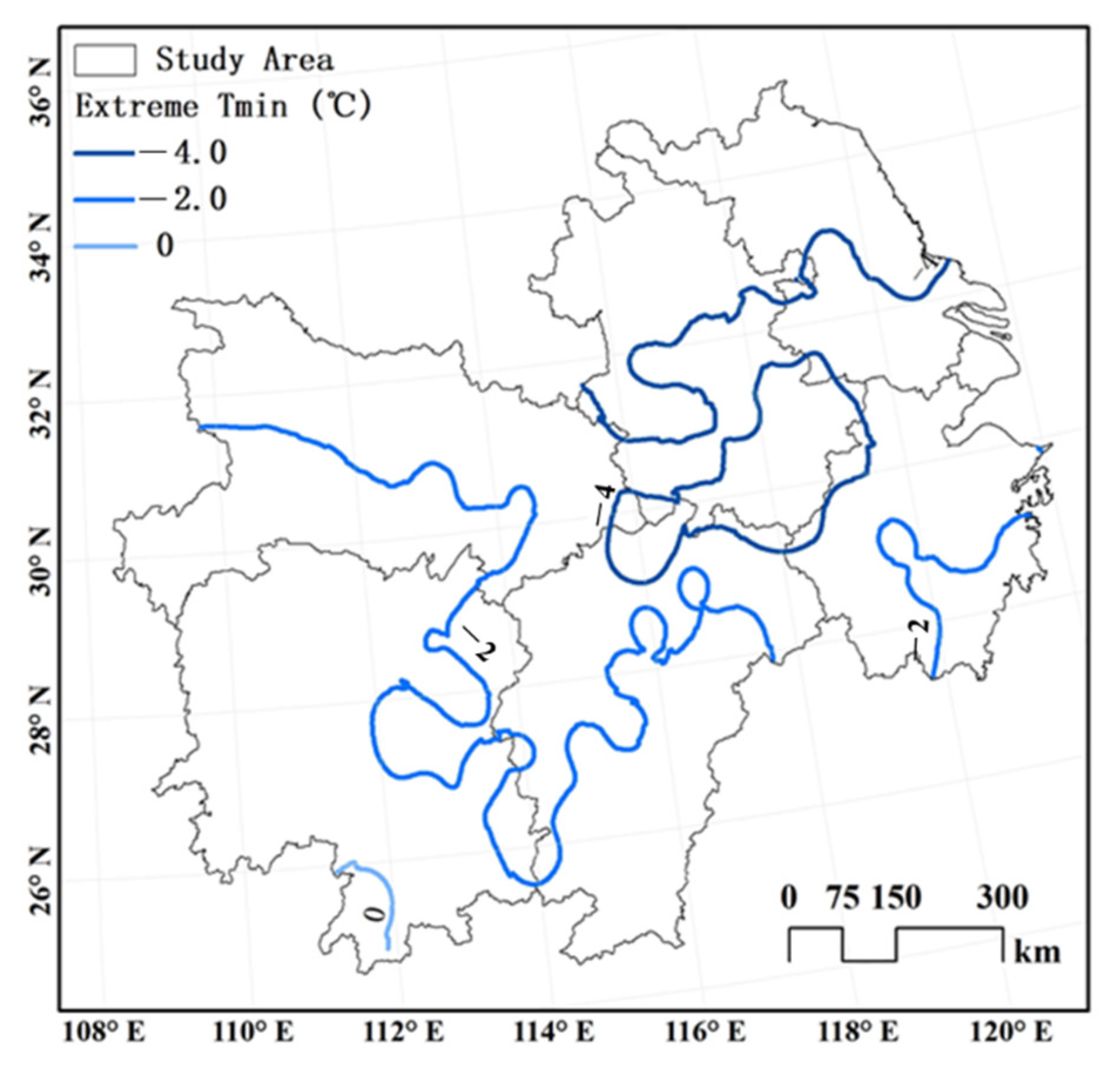
4.2.3. Spatial Distribution of Extreme Tmin

The extreme minimum air temperatures from March to April in 2003–2018 at each meteorological station in the MLRYR were extracted, and temperature contour lines are shown in Figure 6. From Figure 6, we can see that the extreme Tmin values were not higher than 0 °C, showing that the risk of SFD during the past two decades was distributed across the entire MLRYR region. Spatially, the areas with the lowest extreme Tmin (−4 °C), denoted by the dark blue line (Figure 6), were found mainly in the northeastern parts of the study area (Jiangsu and Anhui provinces). Regions with the highest extreme Tmin (0 °C) were very small and were only observed in the southwestern part of the MLRYR. The extreme Tmin values around −2 °C were the most widely distributed values observed in the MLRYR, and occurred in the entire Hubei Province, and almost all of Zhejiang, Jiangxi, and Hunan Provinces. Generally, the contour lines of extreme Tmin were observed to gradually increase from −4 °C in the northeast to 0 °C in the southwest.

4.3. Performance of the Tmin Estimation Model

4.3.1. Validation of the Tmin Estimation Model

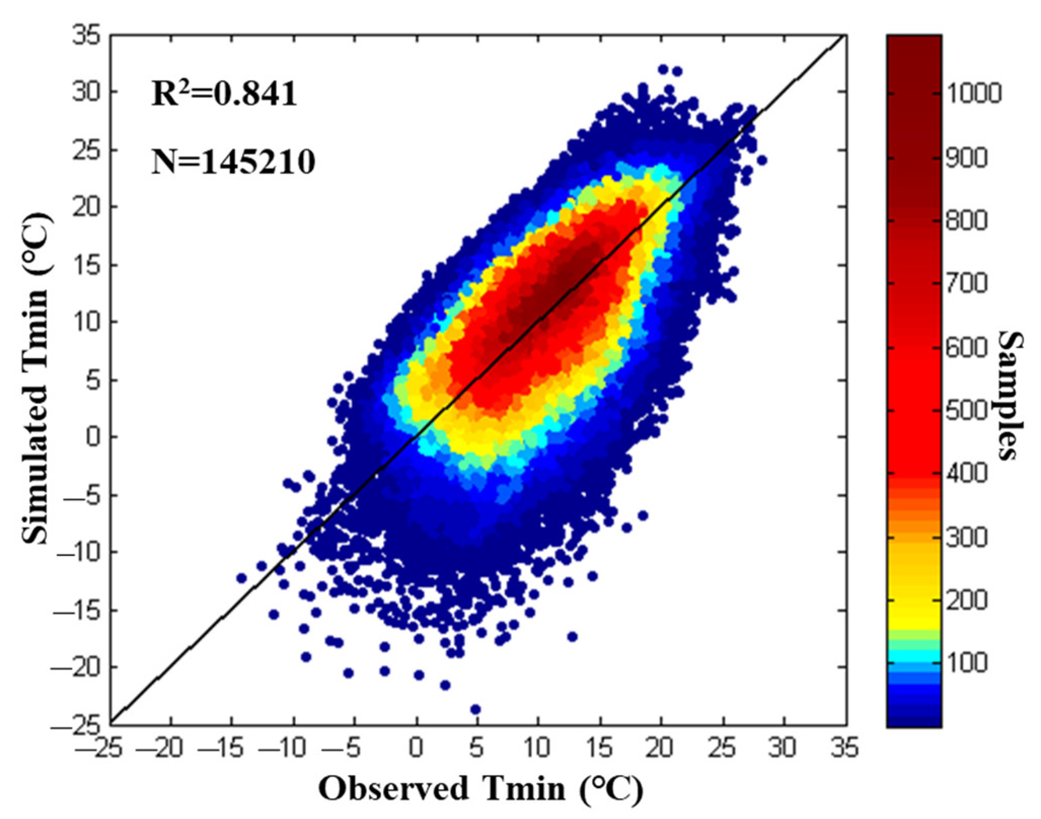
After the three-step process described in Section 3.3, the Tmin estimation model was established based on MODIS reconstructed LST of nighttime MYD11A1 and digital elevation data in the MLRYR. The scatter plot of observed Tmin at ground meteorological stations and Tmin simulated by the established estimation model is displayed in Figure 7. The rainbow colors in the figure show the distribution of the number of samples. Points in warm colors (red, orange) indicate more samples, and cool colors (blues) denote fewer samples. In order to assess the performance of the Tmin estimation model, the three statistics were calculated between 145,210 observed Tmin samples and their corresponding simulated values. The results showed that the R2 value between observed and simulated Tmin was 0.841, much higher than those obtained by different window scales for MYD11A1 nighttime LST products (Figure 3). Similarly, the Tmin estimation model had a lower MAE (1.66 °C) than the MAE values produced by the MYD11A1 nighttime LST products (4.05–5.51 °C). The RMSE values resulting from the Tmin estimation model were also significantly lower than the previously calculated RMSE values (2.15 °C versus 5.37–7.58 °C). Further evaluation for the Tmin estimation model was done by using with NRMSE and EF. Results showed that NRMSE and EF were 25.4% and 0.12, also indicating the model was acceptable.

4.3.2. Difference of Tmin between Observations and Simulations

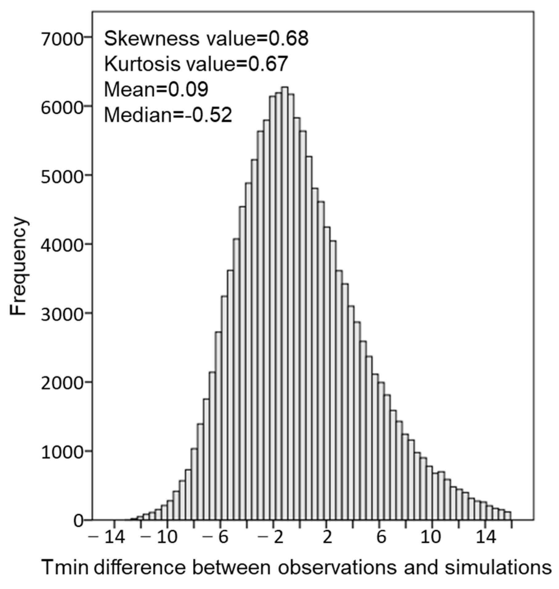
The differences between observed and simulated Tmin were quantified for the entire study area in 2003–2018 by analyzing the distribution shape of the differences. The frequency histogram of these Tmin differences, as well as the accuracy (median, mean, skewness, and kurtosis) are shown in Figure 8. The global distribution of the Tmin differences was centered at 0.09 °C, and the median was slightly left-shifted with a value of −0.52 °C. The frequency distribution of Tmin differences was observed to be bell shaped. Both skewness and kurtosis were greater than zero, indicating a positively skewed distribution with a steep peak.

4.3.3. Performance of the Tmin Estimation Model in Grouped Latitude and Altitude

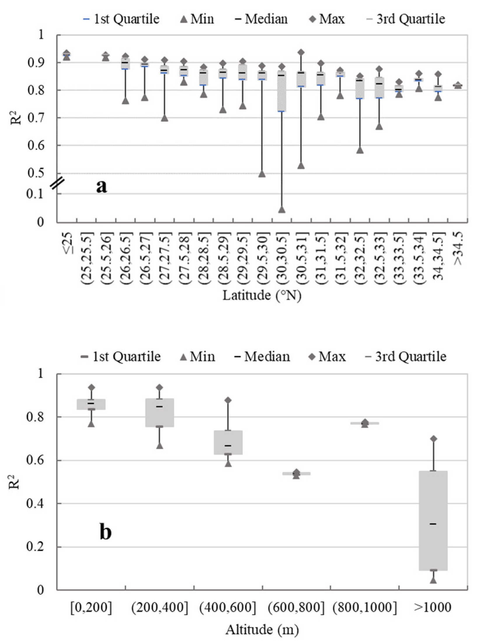
The performance of the Tmin estimation model was evaluated through computing the R2 in different latitudes and altitudes by grouping 163 ground meteorological stations. The latitude at about 0.5°N interval and the altitude at 200 m interval were grouped separately. The variance plots of R2 along with latitude and altitude were shown in Figure 9a,b. The quartiles of all R2 values in different latitudes between observed and simulated Tmin were between 0.70 and 0.95, and the median R2 showed a slightly fluctuant decreasing trend with the increasing of latitude (Figure 9a). The minimum R2 appeared in the latitude between 30 and 30.5° N, with the value of being less than 0.1. The majority reason for such a low R2 may be the high altitude, where the altitude is more than 1000 m. Meanwhile, the R2 values in different altitudes were also exhibited in Figure 9b, and it similarly showed the declining characteristics with the elevated altitude. The minimum R2, the minimum quartile, and the minimum median all appeared in the high-altitude areas above 1000 m. Fortunately, the tea gardens were mostly distributed in hills and mountains with an altitude of being 200–1000 m, and the R2 values were greater than 0.65 except for the altitude between 600 and 800 m. For the higher mountains with the altitude of above 1000 m, recommended lapse rates in different altitudes and aspects can be found in Meteorological Industry Standard [26].

4.4. Characteristics of SFD for Tea Plants in a Typical Frost Year

4.4.1. Temporal Characteristics of Tmin for a Typical Cooling Period

Average Tmin over the MLRYR from March to April in 2006 tended to increase gradually over time, with occasional periods of sharp decreases followed by rapid increases (Figure 10). The "Yearbook of Meteorological Disasters in China" (2007) [46] recorded the following observations: “The cold air was more active in the spring of 2006. From March to April, most regions of China were hit by cold waves from north to south. The temperature at nine individual stations dropped more than 12 °C (data not shown in our Figure 10). The minimum air temperature in the central and northern regions of Yangtze River dropped to about 0 °C. The lower temperatures were detrimental to the normal growth of overwintering crops and some early spring crops, such as early rice and tea plants, and those crops suffered frost damage.”
The temporal dynamics of Tmin over the MLRYR (Figure 10) showed two significant cooling periods around mid-March and mid-April. Several other periods of small fluctuations in Tmin were also observed from March to April (Figure 10). The two significant cooling periods occurring around mid-March and mid-April, and one slightly cooling period appearing at the end of March were mentioned in the "Yearbook of Meteorological Disasters in China" (2007) [46]. The percentage of meteorological stations with daily Tmin less than 4 °C (referred to as station ratio in Figure 10) displayed three small peaks (excluding the first three days of the record shown). The first cooling period in mid-March was the most significant, when more than 60% of the stations reported Tmin less than 4 °C for three consecutive days. Even though the temperature dropped significantly during the third cooling period (mid-April), the percentage of meteorological stations that had daily Tmin below the threshold of SFD (4°) was not high (<15%) due to the relatively higher temperatures in the previous days.

4.4.2. Spatial Distribution of Daily Minimum Air Temperature in Three Cooling Periods

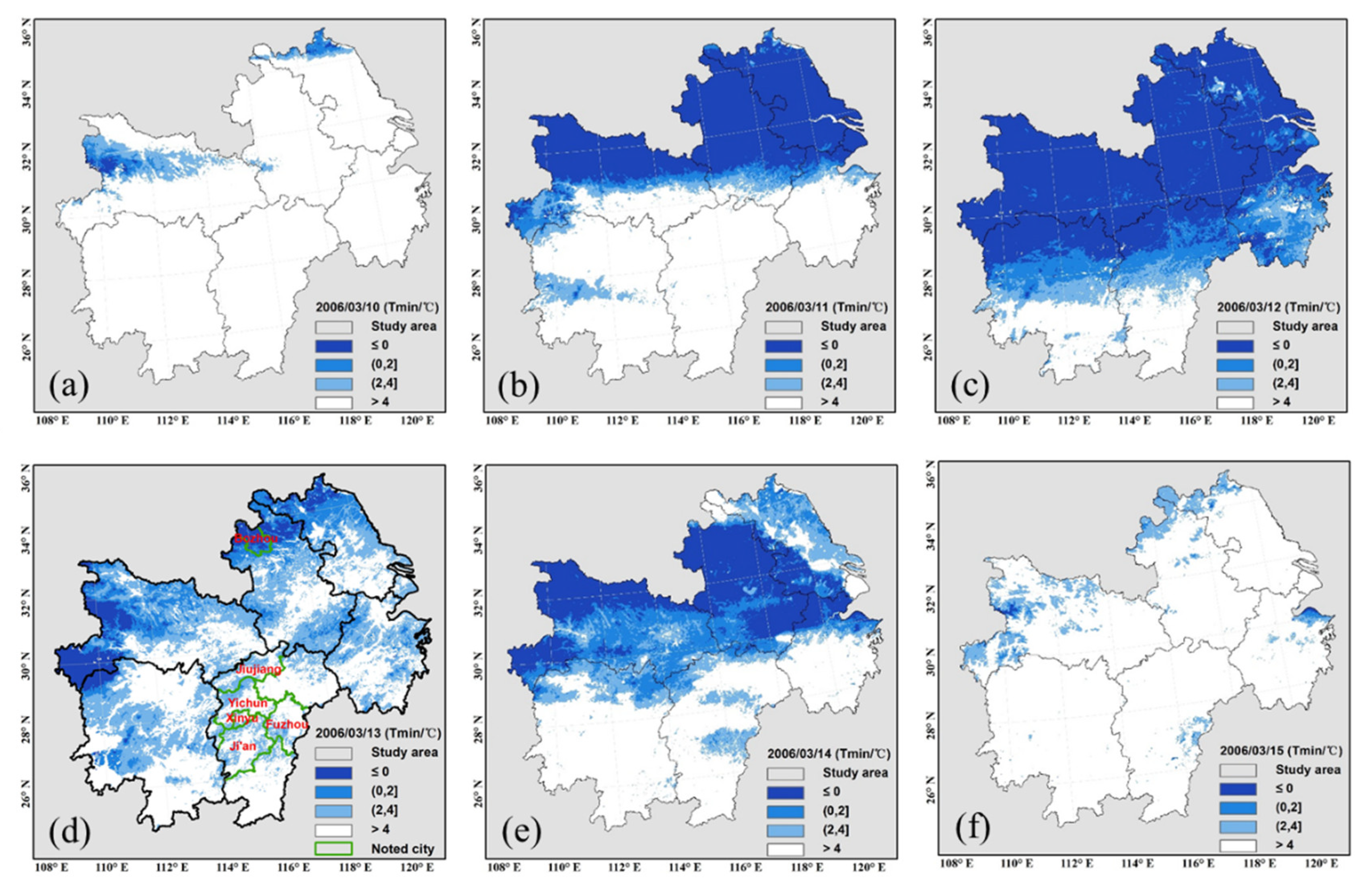
The spatial distributions of simulated daily Tmin during three cooling periods in March and April 2006 are shown in Figure 11, Figure 12 and Figure 13. The first cooling period appeared on 10–14 March 2006. The "Yearbook of Meteorological Disasters in China" (2007) [46] recorded: “A strong cold wave occurred on 10–14 March 2006. The temperature dropped by 12–18 °C during March 11–13, and snow appeared in more than 22 counties distributed in Yichun, Xinyu, Ji’an, Fuzhou, and Jiujiang cities in Jiangxi Province. This strong cooling process caused 119,000 hm2 of crops to be damaged, and its direct agricultural economic losses were more than 100 million RMB in Jiangxi Province. Meanwhile, in the northeastern part of Anhui Province, the minimum air temperature of Bozhou City dropped to −2 to −4 °C, and nearly 60,000 hm2 of crops suffered freezing damage.” Daily minimum air temperature simulated by the Tmin estimation model perfectly revealed the cooling progression over this period (Figure 11). On March 10, frost damage sporadically appeared in the northern portion of the study area (Figure 11a). As the cold wave moved to the south, the cooling intensity significantly increased, and the affected regions spatially enlarged from March 11 to March 14 (Figure 11b–e). All regions in the six cities referred to in the "Yearbook of Meteorological Disasters in China" (2007) were accurately identified as suffering SFD (Figure 11d, administrative boundaries marked in green). There were no disaster records for March 15 in public reports. Correspondingly, the regions suffering from SFD were significantly reduced compared with several days earlier (Figure 11f). Tmin simulated with the MODIS nighttime reconstructed LST product perfectly exhibited this cooling process occurring over several days.
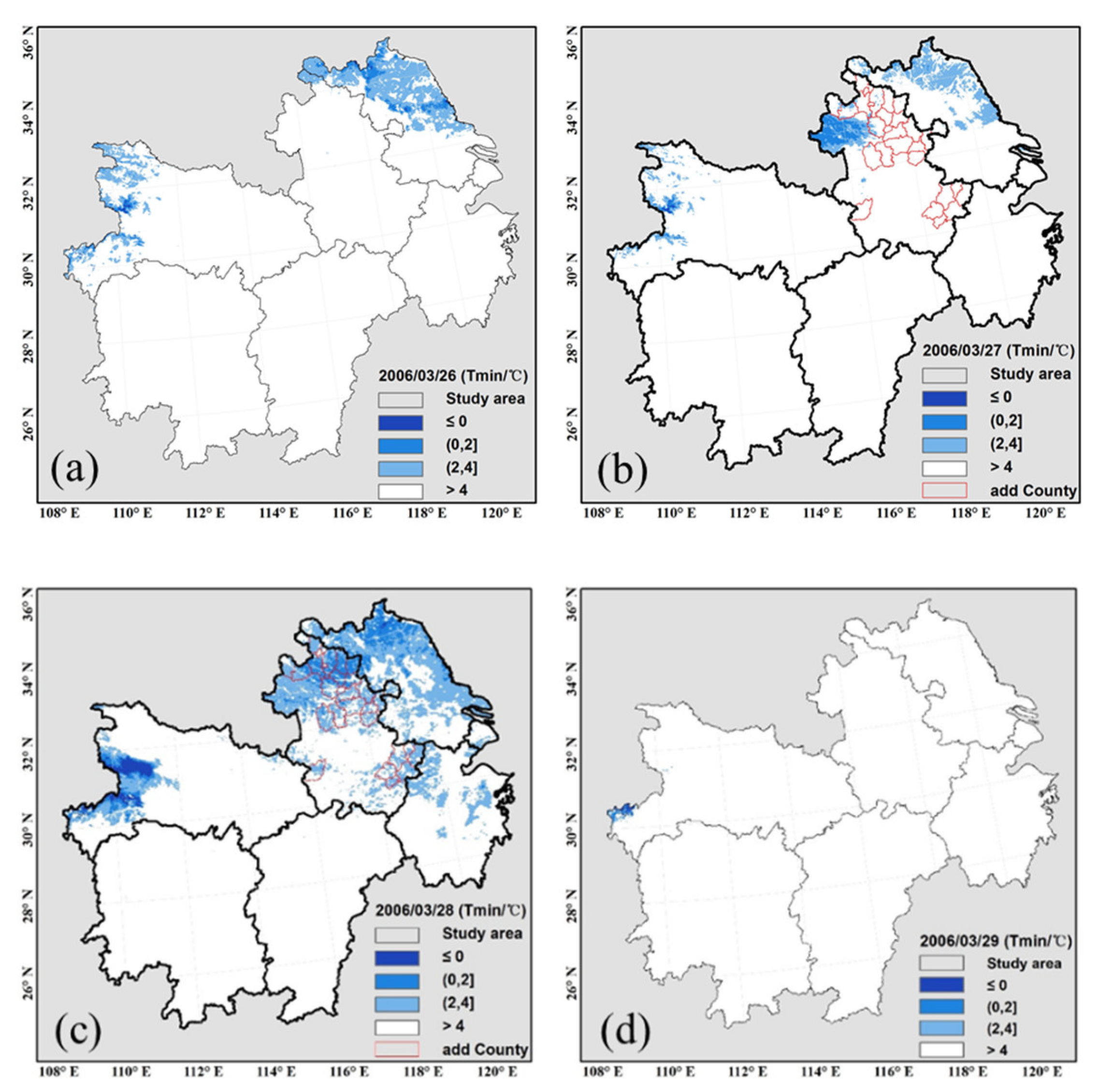
The second cooling period occurred on 26–28 March 2006. The "Yearbook of Meteorological Disasters in China" (2007) [46] recorded: “On March 27−28, strong northerly winds occurred in parts of Jiangsu Province, and the maximum cooling range reached to 10 °C. On the evening of March 27, there were about 27 counties in Anhui Province that experienced strong winds and cooling process. The areas affected by this cooling process were up to 17,000 hm2, and its direct economic loss reached up to 130 million RMB.” According to the disaster records, the regions affected by this cooling process were mainly in Anhui and Jiangsu Provinces. The spatial distribution of simulated daily Tmin from March 26 to 29 precisely exhibited this evolution process (Figure 12). From March 27 to 28, the cooling areas noticeably enlarged in Anhui and Jiangsu Provinces. Especially the counties identified by red boundaries (Figure 12b,c) in Anhui Province were exactly consistent with disaster records. The cooling period ended on March 29, and the regions in the MLRYR affected by SFD were almost gone.
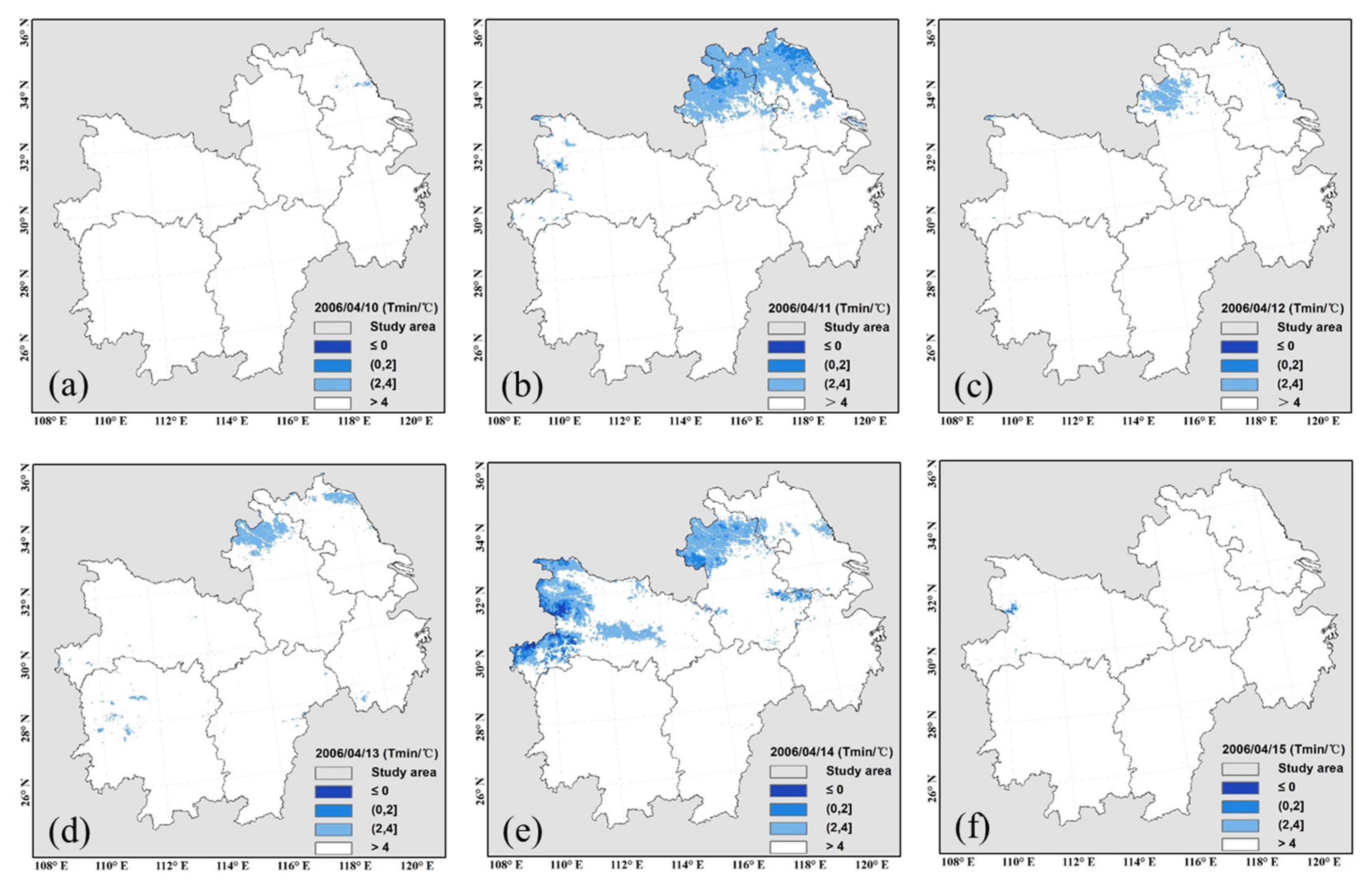
The last cooling period occurred on 10–15 April 2006. This cooling period affected Jiangsu and Hubei Provinces and was recorded in the "Yearbook of Meteorological Disasters in China" (2007) [46], as follows: “With the increase of temperature in April, there were fewer stations where the temperature dropped to the threshold for SFD to tea plant, and the impacted regions were also smaller.” There was only one day when the proportion of meteorological stations within the MLRYR with daily Tmin of less than 4 °C exceeded 10% during this cooling period (Figure 10). The regions with simulated daily Tmin being no higher than 4 °C were scattered in the northern part of MLRYR (Figure 13), and these observations were consistent with the station ratio values demonstrating the limited areal extent of the damaging cold temperatures.

4.4.3. Spatial Distribution of Different Frost Damage Levels for Tea Plants

Based on the spring frost indicator for tea plants in the MLRYR (Table 1), the spatial distributions of SFD for tea plants in the MLRYR during the three cooling periods in 2006 for locations identified as shrub PFT are shown in Figure 14. Overall, the impact of spring frost during the first cooling period was the greatest. The regions with severe spring frost, denoted by the dark blue color (Figure 14), were distributed mainly in the northern part of MLRYR. Areas categorized as having light SFD were relatively smaller and were concentrated in the southern parts of Zhejiang Province, and central parts of Hunan and Jiangxi Provinces. There were almost no areas suffering moderate SFD. These areas were scattered in the border area of Jiangxi and Zhejiang Provinces. Although the area influenced by damaging frost was extensive during the first cooling period, there were still small regions located in the southern part of the study area that were not affected by SFD. The damaging effects of frost during the other two cooling periods were relatively smaller. The affected areas of SFD were mainly concentrated in the northwestern part of the study area. In particular, the regions affected by severe spring frost were found to be scattered in the northwestern part of the study region, corresponding to parts of the Daba Mountains and Wushan Mountains.

5. Discussion and Limitations

5.1. Factors Influencing the Minimum Air Temperature Estimation Model

The major weather-related hazard to tea plant production is SFD caused by low temperatures. Research regarding SFD to tea plants has been limited by the number of meteorological stations and their distribution. Temperature observations at ground meteorological stations are often difficult to monitor and evaluate precisely over a large spatial extent. Previous research mainly focused on the spatiotemporal distribution and risk assessment of SFD in provincial scale during several decades [23,60,61]. High-resolution impact assessment of SFD on tea plants over a large-scale region is hard to do based on ground-based meteorological observations. Remotely sensed land surface temperature products are one of the most suitable choices to monitor and evaluate the effects of SFD to tea plants. However, neither the Terra satellite nor the Aqua satellite had overpass times that corresponded to the time of lowest daily temperature, i.e., around sunrise. Therefore, it was necessary to develop a minimum air temperature estimation model based on high spatial resolution LST products. Although the validation results evaluated by R2, MAE, RMSE, NRMSE, and EF showed that the Tmin estimation model was reasonable and credible, there were still several limitations that restricted simulation accuracy.

5.1.1. Weather Conditions

One of the limitations of the Tmin estimation model was that the relationship between Tmin observations at ground meteorological stations and MODIS LST products retrieved from the generalized split window algorithm [43] was restricted by weather conditions. It is well documented that the soil emits longwave radiation energy during nighttime hours. During this radiative cooling process, the land surface temperature becomes lower and lower. Longwave radiation energy emitted by the soil is affected by the processes of thermal conduction and water phase change before sunrise [62]. The minimum air temperature appears around sunrise when the thermal energy emitted by the ground surface is balanced by incoming solar radiation. In actuality, the longwave radiation energy emitted from soil will vary with weather conditions, such as sunny, cloudy, and rainy days. The MODIS LST products were retrieved under clear-sky conditions [63]. Therefore, the minimum air temperature estimated based on nighttime LST products, theoretically, may have small underestimation or overestimation errors due to the influence of weather conditions.

5.1.2. Land Cover Types

Another limitation of the Tmin estimation model was that the impacts of land cover type and their components on minimum air temperature in mixed pixels were not considered. Previous studies have shown that the diurnal temperature variation of component temperatures for different land cover types were distinct, especially for different fractional vegetation cover [59,64,65]. In this study, the land cover types surrounding meteorological stations were not considered either at 1-km scale (central pixel for MODIS LST products) or at 3-km (3 × 3 pixels) scale. Although ground meteorological stations and their surroundings were covered by grassland in China, fields are fragmented in the MLRYR, and their land cover types are diverse over more than 1-km scale. There may exist large numbers of mixed pixels in tea planting areas, even at a spatial resolution of 1 km. Furthermore, some uncertainties with regard to Tmin estimation will be inevitable because of the variation of the diurnal temperature range due to the combined effects of vegetation cover fraction, land cover types, and soil moisture [59,66].

5.1.3. DEM

An additional limitation of the Tmin estimation model was that the effects of elevation on minimum air temperature were not considered. Turbulent exchange depends largely on the changes of terrain. Compared with flat and concave land areas, convex land areas have greater air movement and strong turbulent exchange. Therefore, temperatures can fall more rapidly after sunset than temperatures over flat and concave lands (Means, Tiffany. “Understanding Diurnal Temperature Range.” httpa://thoughtco.com/diurnal-temperature-range-3444244. Last visited on 26 August 2020). As such, the diurnal temperature variation was different over different terrain conditions. Tea plantations in MLRYR are mainly located in hilly areas with gentle slope. The impacts of DEM, theoretically, on SFD for tea plants were relatively limited. Even though, more work should be done in the future to improve the Tmin estimation accuracy by considering the impacts of aspect on Tmin.

5.2. Indicators of SFD for Tea Plants

Damage indicators are the basis for monitoring disaster, forecasting risk, and evaluating impact. Previous studies have classified SFD to tea plants into three categories according to data sources: morphological indicators, physiological indicators, and meteorological indicators. Moreover, meteorological indicators can be further subdivided into daily scale and hourly scale indicators based on the meteorological data availability [67]. In this study, minimum air temperatures at daily scale were used to study SFD to tea plants. This indicator was established based on the dynamic process of frost damage rate [54], taking Longjing 43 (a kind of shrub tea plant with medium and small leaves) as an example. Actually, a similar spring frost process may result in different damage levels for different tea varieties. Therefore, more work should be done to refine the indicators of SFD for more tea varieties, more tea leaf shapes, and more complex terrain. Fortunately, shrub tea plants with medium and small leaves are the dominant type of tea plants in the MLRYR. We believe that the indicator used in this study was suitable for evaluating spatiotemporal characteristics of SFD to tea plants in the MLRYR.
In terms of the time scale of the indicators, meteorological industry standards [26] have established the indicator of SFD for medium and small leaf tea plants based on hourly Tmin and its duration. Hourly scale indicators of SFD have been successfully used to quantitatively evaluate the impacts of SFD on tea plants in Quzhou city, Zhejiang Province. The evaluation results indicated that the individual cases of SFD from 2005 to 2015 were consistent with the actual disaster situation [68]. Tao et al. [69] evaluated the economic losses caused by the SFD to tea plants in northern Jiangxi Province in 2018 based on hourly scale indicators, which was also consistent with the actual disaster losses. From an application point of view, frost damage assessment over a small region requires finer indicators at tiny time scale and more refined temperature data at high spatial resolution. Consequently, hourly LST at high spatial resolution is essential in evaluating SFD over a small area. Research on reconstructing hourly LST data based on remotely sensed LST products will become the focus of follow-up work.

5.3. Tea Planting Area

The MLRYR region, including six provinces and one municipality, was analyzed as a single area. The total land area in the MLRYR exceeds 1,010,000 km2, and the tea plantation area was only 10,541 km2 in 2019 [70], accounting for 1.04% of the total land area. However, the areas of shrub extracted by the PFT legend in the MODIS MCD12Q1 product accounted for 4.99% of the total area, and this was much higher than the proportion of the MLRYR planted to tea. Therefore, the spatial distribution of different SFD levels shown and discussed in Section 4.4.3 in this study may include other plants to some degree, such as Camellia oleifera Abel., Forsythia suspensa, Jasminum nudiflorum Lindl., and so on. In the previous studies, Google high-resolution satellite data was used to extract the refined tea plantations over a country [71]. If the study area is expanded to the municipal, provincial, or regional scale, it will become very difficult to preciously extract tea plantation. Almost all publications divided the regional frost levels over the whole study area, without marking the distribution of tea plantation [68,69]. Therefore, additional work should be done to exactly distinguish the tea plantation area in the future, so as to accurately monitor and objectively evaluate the impacts of SFD on tea plants.

6. Conclusions

This study established a minimum air temperature estimation model based on MODIS nighttime reconstructed LST values and digital elevation, and further analyzed the spatiotemporal characteristics of SFD by referring to the indicators of SFD for tea plants in the MLRYR of China. Results showed that the best correlation between Tmin and two LST nighttime products at six window scales was found using the MYD11A1 product at the 3 × 3 pixel window, for which the R2, RMSE, and MAE were 0.782, 5.37 °C, and 4.05 °C, respectively. The Tmin estimation model used a very simple expression to achieve relatively accurate simulations. The RMSE and MAE of estimated Tmin were 2.15 °C and 1.66 °C, respectively, when using more than 100,000 observations at ground meteorological stations. The analysis in a typical frost year (2006) revealed that the estimated Tmin values closely aligned with written historical disaster records. The primary cooling periods recorded in the "Yearbook of Meteorological Disasters in China" were exactly identified, especially for several highlighted cities and counties during the first two cooling periods. This study confirmed that estimated Tmin based on MYD11A1 nighttime products and DEM is a useful way to monitor and evaluate SFD to tea plants in the MLRYR. The MODIS LST products are easy to obtain via EOSDIS and can be used to research and timely quantify SFD over a large spatial extent. The Tmin estimates in detailed temporal and spatial characteristics will be an important consideration for taking effective frost prevention measures at the appropriate time and precise region.

Author Contributions

Conceptualization, P.W. and Z.H.; methodology, P.W.; software and data curation, Y.M. and D.W.; validation, J.T., H.C. and Z.J.; writing—original draft preparation, P.W.; writing—review and editing, P.W.; funding acquisition, P.W. All authors have read and agreed to the published version of the manuscript.

Funding

The research was financially supported by the National Key Research and Development Program of China (2019YFD1002203) and the National Natural Science Foundation of China (31771672).

Informed Consent Statement

Informed consent was obtained from all subjects involved in the study.

Data Availability Statement

All data used during the study area available at http://data.cma.cn/site/index.html, https://earthdata.nasa.gov/ (accessed on 17 March 2021).

Conflicts of Interest

The authors declare no conflict of interest.

References

  1. Roy, S.; Das, S.; Handique, G.; Mukhopadhysy, A.; Muraleedharan, N. Ecology and management of the black inch worm, Hyposidra talaca Walker (Geometridae: Lepidoptera) infesting Camellia sinensis (Theaceae): A review. J. Intergrative Agric. 2017, 16, 2115–2127. [Google Scholar] [CrossRef]
  2. Weng, K.; Xi, X.J.; Wan, X.C.; Zhao, Y.X.; Li, L.X.; Sun, W.J.; Zhang, Y.L. Classification of Tea; GB/T 30766-2014; State Administration for Market Regulation and Standardization Administration: Beijing, China, 2014. (In Chinese) [Google Scholar]
  3. Paiva, L.; Lima, E.; Motta, M.; Marcone, M.; Baptista, J. Variability of antioxidant properties, catechins, caffeine, L-theanine and other amino acids in different plant parts of Azorean Camellia sinensis. Curr. Res. Food Sci. 2020, 3, 227–234. [Google Scholar] [CrossRef] [PubMed]
  4. Jin, Z.F.; Yao, Y.P. Research on Key Technique of Meteorological Support for the Tea Production in Regions South of the Yangtze River; China Meteorological Press: Beijing, China, 2017. (In Chinese) [Google Scholar]
  5. FAO. FAOSTAT Database; FAO: Rome, Italy, 2020; Available online: http://www.fao.org/faostat/en/#data/QC (accessed on 19 August 2020).
  6. Sun, X.B.; Tao, S.H.; Tian, Q.; Cao, S.X.; Liu, R.N.; Wang, Z.Q.; Chen, X.X. Forecast of first plucking date of spring tea and evaluation of tea climate quality grade in Jingxian, Anhui. Chin. Agric. Sci. Bull. 2017, 33, 49–54, (In Chinese with English abstract). [Google Scholar]
  7. Wang, J.Z.; Huang, J.C.; Wang, S.; Chen, Y.Y.; An, X.J.; Zhang, L.J. Effects of light and temperature factors on quality tea of Meitancuiya in Spring. Guizhou Agric. Sci. 2019, 47, 108–112, (In Chinese with English abstract). [Google Scholar]
  8. Jin, J.; Diao, X.G.; Feng, H.Q. The status and development trend forecast of Zhejiang tea industry in 2019. China Tea. 2020, 3, 53–57. [Google Scholar]
  9. IPCC. Summary for policymakers. In Climate Change 2013: The Physical Science Basis. Contribution of Working Group I to the Fifth Assessment Report of the Intergovernmental Panel on Climate Change; Stocker, T.F., Qin, D., Plattner, G.-K., Tignor, M., Allen, S.K., Boschung, J., Nauels, A., Xia, Y., Bex, V., Midgley, P.M., Eds.; Cambridge University Press: Cambridge, UK; New York, NY, USA, 2013; p. 1535. [Google Scholar]
  10. Kodra, E.; Steinhaeuser, K.; Ganguly, A.R. Persisting cold extremes under 21st-century warming scenarios. Geophys. Res. Lett. 2011, 38, 99–106. [Google Scholar] [CrossRef] [Green Version]
  11. Augspurger, C.K. Reconstructing patterns of temperature, phenology, and frost damage over 124 years: Spring damage risk is increasing. Ecology 2013, 94, 41–50. [Google Scholar] [CrossRef] [PubMed]
  12. Rigby, J.R.; Porporato, A. Spring frost risk in a changing climate. Geophys. Res. Lett. 2008, 35, L12703. [Google Scholar] [CrossRef]
  13. Snyder, R.L. Principles of Frost Protection. 2000. Available online: http://biomet.ucdavis.edu/frostprotection/Principles%20of%20Frost%20Protection/FP005.html (accessed on 24 August 2020).
  14. Barlow, K.M.; Christy, B.P.; O’Leary, G.J.; Riffkin, P.A.; Nuttall, J.G. Simulating the impact of extreme heat and frost events on wheat crop production: A review. Field Crop. Res. 2015, 171, 109–119. [Google Scholar] [CrossRef] [Green Version]
  15. Zhao, L.C.; Li, Q.Z.; Zhang, Y.; Wang, H.Y.; Du, X. Normalized NDVI valley area index (NNVAI)-based framework for quantitative and timely monitoring of winter wheat frost damage on the Huang-Huai-Hai Plain, China. Agric. Ecosyst. Environ. 2020, 292, 106793. [Google Scholar] [CrossRef]
  16. Reinsdorf, E.; Koch, H.J. Modeling crown temperature of winter sugar beet and its application in risk assessment for frost killing in Central Europe. Agric. For. Meteorol. 2013, 182–183, 21–30. [Google Scholar] [CrossRef]
  17. Pulatov, B.; Linderson, M.; Hall, K.; Jönsson, A.M. Modeling climate change impact on potato crop phenology, and risk of frost damage and heat stress in northern Europe. Agric. For. Meteorol. 2015, 214–215, 281–292. [Google Scholar] [CrossRef]
  18. Vitasse, Y.; Schneider, L.; Rixen, C.; Christen, D.; Rebetez, M. Increase in the risk of exposure of forest and fruit trees to spring frosts at higher elevations in Switzerland over the last four decades. Agric. For. Meteorol. 2018, 248, 60–69. [Google Scholar] [CrossRef]
  19. Kotikot, S.M.; Flores, A.; Griffin, R.E.; Sedah, A.; Nyaga, J.; Mugo, R.; Limaye, A.; Irwin, D.E. Mapping threats to agriculture in East Africa: Performance of MODIS derived LST for frost identification in Kenya’s tea plantations. Int. J. Appl. Earth Obs. Geoinf. 2018, 72, 131–139. [Google Scholar] [CrossRef]
  20. Awaya, Y.; Tanaka, K.; Kodani, E.; Nishizono, T. Responses of a beech (Fagus crenata Blume) stand to late spring frost damage in Morioka, Japan. For. Ecol. Manag. 2009, 257, 2359–2369. [Google Scholar] [CrossRef]
  21. Bascietto, M.; Bajocco, S.; Mazzenga, F.; Matteucci, G. Assessing spring frost effects on beech forests in Central Apennines from remotely-sensed data. Agric. For. Meteorol. 2018, 248, 240–250. [Google Scholar] [CrossRef]
  22. Allevato, E.; Saulino, L.; Cesarano, G.; Chirico, G.B.; D’Urso, G.; Bolognesi, S.F.; Rita, A.; Rossi, S.; Saracino, A.; Bonanomi, G. Canopy damage by spring frost in European beech along the Apennines: Effect of latitude, altitude and aspect. Remote Sens. Environ. 2019, 225, 431–440. [Google Scholar] [CrossRef]
  23. Jin, Z.F.; Ye, J.G.; Yang, Z.Q.; Sun, R.; Hu, B.; Li, R.Z. Climate suitability for tea growing in Zhejiang Province. Chin. J. Appl. Ecol. 2014, 25, 967–973, (In Chinese with English abstract). [Google Scholar] [CrossRef]
  24. Wu, Y.; Jin, Z.F.; Ye, J.G.; Yang, Z.Q.; Hu, B.; Li, R.Z. Teleconnection analysis between spring frost damage on tea in Zhejiang Province and sea surface temperature in Pacific. Chin. J. Agrometeorol. 2014, 35, 434–439, (In Chinese with English abstract). [Google Scholar] [CrossRef]
  25. Li, R.Z.; Jin, Z.F.; Yang, Z.Q.; Wang, Z.H.; Yao, Y.P. Revision on meteorological indices of spring frost disaster for Camellia Sinensis in Zhejiang Province. Chin. J. Ecol. 2016, 35, 2659–2666, (In Chinese with English abstract). [Google Scholar]
  26. Jin, Z.F.; Yao, Y.P.; Gao, L.; Wang, Z.H.; Yu, L.Y.; Chen, H.; Li, R.Z. Grade of Frost Damage to Tea Plant; QX/T 410—2017; China Meteorological Administration: Beijing, China, 2017. (In Chinese) [Google Scholar]
  27. Hu, B.; Jin, Z.F.; Yan, J.Z.; Li, R.Z. Temporal and spatial distribution of early spring frost of Camellia Sinensic in Zhejiang Province based on FastICA. Chin. Agric. Sci. Bull. 2014, 30, 190–196, (In Chinese with English abstract). [Google Scholar]
  28. Lou, W.P.; Wu, L.H.; Ji, Z.W. The contribution of climate change to economic output of Wuniuzao spring tea in Shaoxing. Chin. J. Ecol. 2014, 33, 3358–3367, (In Chinese with English abstract). [Google Scholar] [CrossRef]
  29. Jin, Z.F.; Hu, B.; Yan, J.Z.; Yang, Z.Q.; Li, R.Z.; Ye, J.G. Agro-meteorological disaster risk evaluation of tea planting in Zhejiang Province. Chin. J. Ecol. 2014, 33, 771–777, (In Chinese with English abstract). [Google Scholar] [CrossRef]
  30. Zhu, W.B.; Lv, A.F.; Jia, S.F. Estimation of daily maximum and minimum air temperature using MODIS land surface temperature products. Remote Sens. Environ. 2013, 130, 62–73. [Google Scholar] [CrossRef]
  31. Vancutsem, C.; Ceccato, P.; Dunku, T.; Connor, S.J. Evaluation of MODIS land surface temperature data to estimate air temperature in different ecosystems over Africa. Remote Sens. Environ 2010, 114, 449–465. [Google Scholar] [CrossRef]
  32. Pouteau, R.; Rambal, S.; Ratte, J.P.; Gogé, F.; Joffre, R.; Winkel, T. Downscaling MODIS-derived maps using GIS and boosted regression trees: The case of frost occurrence over the Arid Andean Highlands of Bolivia. Remote Sens. Environ. 2011, 115, 117–129. [Google Scholar] [CrossRef] [Green Version]
  33. Lin, S.P.; Moore, N.J.; Messina, J.P.; Devisser, M.H.; Wu, J.P. Evaluation of estimating daily maximum and minimum air temperature with MODIS data in east Africa. Int. J. Appl. Earth Obs. Geoinf. 2012, 18, 128–140. [Google Scholar] [CrossRef]
  34. Zeng, L.L.; Wardlow, B.D.; Tadesse, T.; Shan, J.; Hayes, M.J.; Li, D.R.; Xiang, D.X. Estimation of Daily Air Temperature Based on MODIS Land Surface Temperature Products over the Corn Belt in the US. Remote Sens. 2015, 7, 951–970. [Google Scholar] [CrossRef] [Green Version]
  35. Fu, G.; Shen, Z.X.; Zhang, X.Z.; Shi, P.L.; Zhang, Y.J.; Wu, J.S. Estimating air temperature of an alpine meadow on the Northern Tibetan Plateau using MODIS land surface temperature. Acta Ecol. Sin. 2011, 31, 8–13. [Google Scholar] [CrossRef]
  36. Wang, P.J.; Gao, F.; Masek, J.G. Operational data fusion framework for building frequent Landsat-like imagery. IEEE Trans. Geosci. Remote Sens. 2014, 52, 7353–7365. [Google Scholar] [CrossRef]
  37. Rao, Y.H.; Liang, S.L.; Wang, S.D.; Yu, Y.Y.; Song, Z.; Zhou, Y.; Shen, M.G.; Xu, B.Q. Estimating daily average surface air temperature using satellite land surface temperature and top-of-atmosphere radiation products over the Tibetan Plateau. Remote Sens. Environ. 2019, 234, 111462. [Google Scholar] [CrossRef]
  38. Xu, Y.M.; Shen, Y. Reconstruction of the land surface temperature time series using harmonic analysis. Comput. Geosci. 2013, 61, 126–132. [Google Scholar] [CrossRef]
  39. Sun, L.; Chen, Z.X.; Gao, F.; Anderson, M.; Song, L.S.; Wang, L.M.; Hu, B.; Yang, Y. Reconstructing daily clear-sky land surface temperature for cloudy regions from MODIS data. Comput. Geosci. 2017, 105, 10–20. [Google Scholar] [CrossRef]
  40. Zhang, Y.F.; Chen, Y.H.; Li, Y.; Xia, H.P.; Li, J. Reconstructing One Kilometre Resolution Daily Clear-Sky LST for China’s Landmass Using the BME Method. Remote Sens. 2019, 11, 2610. [Google Scholar] [CrossRef] [Green Version]
  41. Zhao, W.; Duan, S.B. Reconstruction of daytime land surface temperatures under cloud-covered conditions using integrated MODIS/Terra land products and MSG geostationary satellite data. Remote Sens. Environ. 2020, 247, 111931. [Google Scholar] [CrossRef]
  42. Ding, Y.M.; Wang, W.G.; Song, R.M.; Shao, Q.X.; Jiao, X.Y.; Xing, W.Q. Modeling spatial and temporal variability of the impact of climate change on rice irrigation water requirements in the middle of lower reaches of the Yangtze River, China. Agric. Water Manag. 2017, 193, 89–101. [Google Scholar] [CrossRef]
  43. Wan, Z.M.; Zhang, Y.L.; Zhang, Q.C.; Li, Z.L. Validation of the land-surface temperature products retrieved from Terra Moderate Resolution Imaging Spectroradiometer data. Remote Sens. Environ. 2002, 83, 163–180. [Google Scholar] [CrossRef]
  44. Sulla-Menashe, D.; Friedl, M.A. User guide to collection 6 MODIS Land Cover (MCD12Q1 and MCD12Q2) Product. 2018. Available online: https://lpdaac.usgs.gov/documents/101/MCD12_User_Guide_V6.pdf (accessed on 7 January 2021).
  45. Abrams, M.; Crippen, R. User Guide of ASTER GDEM V3. 2019. Available online: https://catalog.data.gov/dataset/aster-global-digital-elevation-model-v003 (accessed on 17 March 2021).
  46. Dong, W.J. Yearbooks of Meteorological Disasters in China; China Meteorological Press: Beijing, China, 2007. [Google Scholar]
  47. Jamieson, P.D.; Porter, J.R.; Wilson, D.R. A test of the computer simulation model ARCWheat1 on wheat crops grown in New Zealand. Field Crop. Res. 1991, 27, 337–350. [Google Scholar] [CrossRef]
  48. Nash, J.E.; Sutcliffe, J.V. River flow forecasting through conceptual models part I—A discussion of principles. J. Hydrol. 1970, 10, 282–290. [Google Scholar] [CrossRef]
  49. Wang, E.L.; Martre, P.; Zhao, Z.G.; Ewert, F.; Maiorano, A.; Rötter, R.P.; Kimball, B.A.; Ottman, M.J.; Wall, G.W.; White, J.W.; et al. The uncertainty of crop yield projections is reduced by improved temperature response functions. Nat. Plants 2017, 3, 17102. [Google Scholar] [CrossRef] [Green Version]
  50. Yang, J.Y.; Huo, Z.G.; Wu, L.; Wang, T.Y.; Zhang, G.X. Indicator-based evaluation of spatiotemporal characteristics of rice flood in Southwest China. Agric. Ecosyst. Environ. 2016, 230, 221–230. [Google Scholar] [CrossRef]
  51. Wang, P.J.; Zhou, Y.Y.; Huo, Z.G.; Han, L.J.; Qiu, J.X.; Tan, Y.J.; Liu, D. Monitoring growth condition of spring maize in Northeast China using a process-based model. Int. J. Appl. Earth Obs. Geoinf. 2018, 66, 27–36. [Google Scholar] [CrossRef]
  52. Tang, Y.X.; Guo, J.P. Risk Assessment of Maize Chilling Injury in Northeast China. J. Appl. Meteorol. Sci. 2016, 27, 352–360, (In Chinese with English abstract). [Google Scholar] [CrossRef]
  53. Liu, L.L.; Ji, H.T.; An, J.P.; Shi, K.J.; Ma, J.F.; Liu, B.; Tang, L.; Cao, W.X.; Zhu, Y. Response of biomass accumulation in wheat to low-temperature stress at jointing and booting stages. Environ. Exp. Bot. 2019, 157, 46–57. [Google Scholar] [CrossRef]
  54. Wang, X.L. Risk Evaluation Technology Research of Spring frost Injury in Southern Yangtze Tea Areas. Master’s Thesis, Nanjing University of Information Science & Technology, Nanjing, China, 2015. (In Chinese with English abstract). [Google Scholar]
  55. Jiang, Y.M.; Jin, Z.F.; Li, R.Z.; Zhang, Y.H.; Yu, W.J. Temporal and spatial distribution of early spring frost for spring tea in southern Zhejiang. Meteorol. Sci. Technol. 2016, 44, 1066–1077, (In Chinese with English abstract). [Google Scholar]
  56. Xu, J.Q.; Qiu, X.F.; Zeng, Y.; Shi, G.P.; Wei, X.H. Analysis on the characteristics of climate change of spring frost damage on tea in Zhejiang. Jiangsu Agric. Sci. 2018, 46, 101–105, (In Chinese with English abstract). [Google Scholar]
  57. Meng, Z.; Yang, D.; Jin, Z.F.; Wang, Z.H.; Lu, D.B. Effect of low temperature and frost on April 1 on tea product in Zhejiang. J. Zhejiang Agric. Sci. 2019, 60, 1397–1400, (In Chinese with English abstract). [Google Scholar]
  58. Wolfe, R.E.; Nishihama, M. Trends in MODIS geolocation error analysis. In Proceedings of the Earth Observing Systems XIV, San Diego, CA, USA, 2–6 August 2009. [Google Scholar]
  59. Duan, S.B.; Li, Z.L.; Tang, B.H.; Wu, H.; Tang, R.L. Direct estimation of land-surface diurnal temperature cycle model parameters from MSG-SEVIRI brightness temperatures under clear sky conditions. Remote Sens. Environ. 2014, 150, 34–43. [Google Scholar] [CrossRef]
  60. Wang, J.; Kuai, Z.M.; Zhang, X.H. The impact of spatial and temporal evolution in climatology of spring frost on spring tea in Jiangsu Province. Chin. J. Agrometeorol. 2011, 32 (Suppl. 1), 222–226, (In Chinese with English abstract). [Google Scholar]
  61. Liu, R.N.; Chen, P. Occurrence regularity of tea spring frost and its risk distribution in Anhui Province. Meteorol. Sci. Technol. 2016, 44, 1060–1065, (In Chinese with English abstract). [Google Scholar]
  62. Cheruy, F.; Dufresne, J.L.; Mesbah, S.A.; Grandpeix, J.Y.; Wang, F. Role of soil thermal inertia in surface temperature and soil moisture-temperature feedback. J. Adv. Modeling Earth Syst. 2017, 9, 2906–2919. [Google Scholar] [CrossRef]
  63. Wan, Z.M. New refinements and validation of the collection-6 MODIS land-surface temperature/emissivity product. Remote Sens. Environ. 2014, 140, 36–45. [Google Scholar] [CrossRef]
  64. Hu, L.Q.; Sun, Y.; Collins, G.; Fu, P. Improved estimates of monthly land surface temperature from MODIS using a diurnal temperature cycle (DTC) model. ISPRS J. Photogramm. Remote Sens. 2020, 168, 131–140. [Google Scholar] [CrossRef]
  65. Liu, X.Y.; Tang, B.H.; Li, Z.L.; Zhou, C.H.; Wu, W.B.; Rasmussen, M.O. An improved method for separating soil and vegetation component temperatures based on diurnal temperature cycle model and spatial correlation. Remote Sens. Environ. 2020, 248, 111979. [Google Scholar] [CrossRef]
  66. Sun, D.; Pinker, R.T.; Kafatos, M. Diurnal temperature range over the United States: A satellite view. Geophys. Res. Lett. 2006, 33, L05705. [Google Scholar] [CrossRef] [Green Version]
  67. Wang, P.J.; Tang, J.X.; Jin, Z.F.; Ma, Y.P.; Chen, H. Review on Spring Frost Disaster for Tea Plant in China. J. Appl. Meteorol. Sci. 2021, 32, 129–145, (In Chinese with English abstract). [Google Scholar] [CrossRef]
  68. Yu, L.P.; Wang, C.; Wang, Z.H. Quantitative evaluation model of frost disaster in early spring tea in Zhejiang Province. Meteorol. Environ. Sci. 2017, 40, 70–74, (In Chinese with English abstract). [Google Scholar]
  69. Tao, Y.; Yang, A.P.; Duan, L.C.; Zhang, K. Quantitative evaluation of the effect of spring frost disaster on tea production in northern Jiangxi in 2018. Meteorol. Disaster Reduct. Res. 2019, 42, 70–74, (In Chinese with English abstract). [Google Scholar]
  70. National Bureau of Statistics. China Statistical Yearbook 2020; China Statistics Press: Beijing China, 2020.
  71. Shen, T.Q.; Qiu, X.F.; Wei, X.H.; Zhu, X.C.; Xu, J.Q. Risk assessment of tea spring frost disaster in detailed plantation area of tea tree—Taking Songyang County of Zhejiang Province as an example. Jiangsu Agric. Sci. 2019, 47, 262–268. (In Chinese) [Google Scholar]
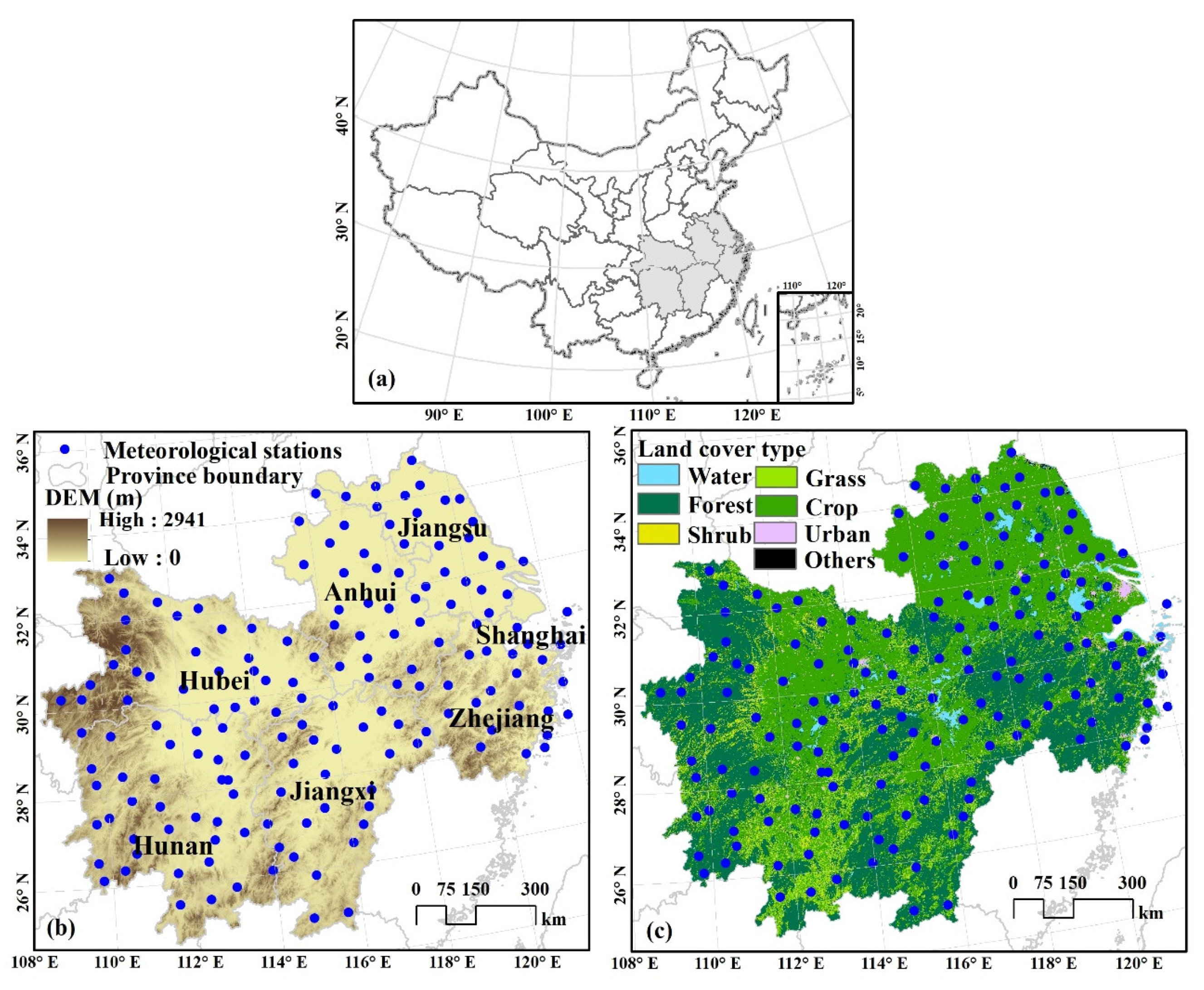
Figure 1. Study area (a), meteorological stations, digital elevation model (DEM) (b), and land cover types in the middle and lower reaches of the Yangtze River region, China (c).
Remotesensing 13 01177 g001
Figure 2. The pipeline and minimum air temperature (Tmin) estimation method. The input data includes meteorological data (describes in Section 2.2.1), MODIS land surface temperature (LST) products (in Section 2.2.2), digital elevation model (DEM) (in Section 2.2.3), and historical disaster records (in Section 2.2.4). The methodology concerns Tmin estimation is composed by MODIS LST reconstruction (in Section 3.1), best window scale selection (in Section 3.2), Tmin regression model based on the standard lapse rate of air temperature (in Section 3.3), and indicators of spring frost damage (SFD) for tea plants (in Section 3.4). The characteristics of SFD for tea plants were exhibited in Section 4.4. Here, T m i n , 0 is the converted Tmin (°C) at sea level, T m i n , 0 is the regressed Tmin (°C) at sea level, and T m i n , d is the estimated Tmin (°C) at local elevation.
Remotesensing 13 01177 g002
Figure 3. Comparison results (a). The coefficient of determination (R2); (b). The root mean square error (RMSE); (c). The mean absolute error (MAE)) between minimum air temperatures (Tmin) and reconstructed land surface temperature (LST) values from MOD11A1 and MYD11A1 nighttime products at different pixel-window scales in the Middle and Lower Reaches of the Yangtze River region, China.
Remotesensing 13 01177 g003
Figure 4. Temporal dynamics of daily minimum air temperature (Tmin) and land surface temperature (LST, from the reconstructed MYD11A1 MODIS LST) from March to April in 2003–2018 over 163 stations in the middle and lower reaches of the Yangtze River region, China.
Remotesensing 13 01177 g004
Figure 5. Daily dynamics of average MYD11A1 nighttime reconstructed land surface temperature (LST) and minimum air temperature (Tmin) from March to April in 2003–2018 over all stations in the middle and lower reaches of the Yangtze River region, China. Sample numbers are the reconstructed LST amounts in daily averaging calculations, and they are shown in the histogram with the right y-axis.
Remotesensing 13 01177 g005
Figure 6. Spatial distribution of extreme minimum air temperature (Tmin) from March to April in 2003–2018 over the middle and lower reaches of the Yangtze River region, China.
Remotesensing 13 01177 g006
Figure 7. Scatter plot of simulated and observed minimum air temperature values (Tmin) from March to April in 2003–2018 in the middle and lower reaches of the Yangtze River region, China.
Remotesensing 13 01177 g007
Figure 8. Frequency distribution of differences between observed and simulated minimum air temperatures (Tmin) from March to April in 2003–2018 in the middle and lower reaches of the Yangtze River region, China.
Remotesensing 13 01177 g008
Figure 9. The box plots of R2 between observed and estimated minimum air temperature (Tmin) grouped 163 ground meteorological stations by latitude (a) and altitude (b) at 0.5° N and 200 m interval separately. The upper and lower boundaries in the gray box represent the 25 and 75 percentiles, the solid line in the gray box represents the medians, and solid triangles and diamonds at the ends of the whiskers represent the minimum and maximum R2 values, respectively.
Remotesensing 13 01177 g009
Figure 10. Temporal dynamics of average minimum air temperatures (Tmin) over the Middle and Lower Reaches of the Yangtze River (MLRYR) region, China from March to April in 2006 (left y-axis). The black error bars denote maximum and minimum values at 163 ground meteorological stations. The hollow, blue-outlined histogram bars (right y-axis) are the percentage of MLRYR stations with daily Tmin less than 4 °C (refer to station ratio, denotes the percentage of meteorological stations with daily Tmin less than 4 °C).
Remotesensing 13 01177 g010
Figure 11. Spatial distribution of simulated daily Tmin on 10–15 March 2006 in the Middle and Lower Reaches of the Yangtze River region, China.
Remotesensing 13 01177 g011
Figure 12. Spatial distribution of simulated daily Tmin on 26–29 March 2006 in the Middle and Lower Reaches of the Yangtze River region, China.
Remotesensing 13 01177 g012
Figure 13. Spatial distribution of simulated daily Tmin on 10–15 April 2006 in the Middle and Lower Reaches of the Yangtze River region, China.
Remotesensing 13 01177 g013
Figure 14. Spatial distribution of different frost damage levels during three cooling periods in 2006 in the Middle and Lower Reaches of the Yangtze River region, China.
Remotesensing 13 01177 g014
Table 1. Definitions of spring frost damage (SFD) levels for tea plants in the Middle and Lower Reaches of the Yangtze River region, China.
Spring Frost DamageDaily Tmin (°C)Duration (d)
Light2–41–5
0–21–3
Moderate2–4≥5
0–23–5
Severe0–2≥5
0≥1
Publisher’s Note: MDPI stays neutral with regard to jurisdictional claims in published maps and institutional affiliations.