Article

Influence of the Low-Frequency Error of the Residual Orbit on Recovering Time-Variable Gravity Field from the Satellite-To-Satellite Tracking Mission

1
State Key Laboratory of Geodesy and Earth’s Dynamics, Innovation Academy for Precision Measurement Science and Technology, Chinese Academy of Sciences, Wuhan 430077, China
2
College of Earth Sciences and Planetary Sciences, University of Chinese Academy of Sciences, Beijing 100049, China
3
School of Geospatial Engineering and Science, Sun Yat-sen University, Zhuhai 519082, China
4
School of Land Science and Technology, China University of Geosciences (Beijing), Beijing 100089, China
5
School of Physics, Huazhong University of Science and Technology, Wuhan 430074, China
*
Author to whom correspondence should be addressed.
Remote Sens. 2021, 13(6), 1118; https://doi.org/10.3390/rs13061118
Submission received: 4 February 2021 / Revised: 4 March 2021 / Accepted: 9 March 2021 / Published: 15 March 2021
(This article belongs to the Special Issue GRACE Satellite Gravimetry for Geosciences)

Abstract

:
When using the dynamic approach to recover the time-variable gravity field, the reference orbit generated by the perturbation model and the non-conservative force observed from the accelerometer should be introduced at first, and then the observation equations of the residual orbit and the residual range rate are established. This introduces a perturbation model error and instrument noise. Thus, there are low-frequency errors in the residual orbit and the residual range rate. Currently, most studies only focus on the low-frequency error of the residual range rate, neglecting the influence of the low-frequency error in the residual orbit. Therefore, under the condition of the perturbation model error and instrument noise including the constant term and 1CPR term, the low-frequency error formulas of the residual orbit and residual range rate are derived according to the characteristics of the solution of the Hill equation. Then, the influence of the low-frequency error on the residuals is analyzed by using the simulation and the real data processing respectively. In the simulation and real data processing, the accuracy of the recovered gravity field can maintain a good consistency for different arc lengths by removing the low-frequency error in the residual orbit. Finally, the time-variable gravity field model UCAS-IGG (University of Chinese Academy of Sciences-Institute of Geodesy and Geophysics) was solved from January 2005 to February 2010 by removing the low-frequency error of the residual orbit and residual range rate. Compared with the official institutions, the UCAS-IGG presents a good consistency in the estimating time-variable gravity field signal. This study demonstrates how the effect of the low-frequency error of the residual orbit should be taken into consideration when the longer arc length is used to recover a time-variable gravity field. Using a long arc length can reduce the variables of the initial state and recover the influence of the small force.

Graphical Abstract

1. Introduction

Since the successful launch of the Gravity Recovery And Climate Experiment (GRACE) mission, research on the time-variable gravity field has made unprecedented achievements [1,2]. The GRACE is mainly equipped with a GNSS receiver, an accelerometer, and microwave ranging to obtain the orbit, the non-conservative acceleration, and the range-rate, respectively to determine the time-variable gravity field model. The methods of recovering the time-variable gravity field mainly include a dynamic approach [3,4,5,6,7,8,9,10], a short arc approach (short arc approach, modified short arc approach, optimized short-arc approach) [11,12,13,14,15], an acceleration approach (point-wise acceleration approach, average acceleration approach) [16,17,18,19], celestial mechanics [20,21] and an energy balance approach [22,23,24,25,26,27]. The accuracy of the time-variable gravity field, which is obtained based on different methods, is basically the same in spatial distribution [13]. The Center for Space Research (CSR) of University of Texas at Austin [4,6], the Jet Propulsion Laboratory (JPL) of National Aeronautics and Space Administration (NASA) [7,28], and the GeoForschungsZentrum (GFZ) [5] represent the three official agencies to deliver GRACE gravity field products.
The essence of the dynamic approach is to generate the reference orbit and reference range rate by using the conservative force model (N-body perturbation, Solid Earth tides, Ocean tide, and so on) and the non-conservative force data observed by the accelerometer, to then obtain the residual orbit and residual range rate by the differences between the GRACE data and the reference data, and build the observation equations of the residual orbit and residual range rate to recover the time-variable gravity field. In fact, the used perturbation model and the non-conservative force are not consistent with the real forces on the satellite. This leads to the perturbation model error and instrument noise. Thus, the residual range rate includes the low-frequency error [29]. The low-frequency error can propagate globally during orbit integration and accelerometer calibration procedure, and could cause errors at low degrees [30]. For the low-frequency error, Tapley et al. [3], Visser [31], Bruinsma et al. [32], Liu et al. [18,19], Meyer et al. [33], Ditmar et al. [34], Hashemi Farahani et al. [35], Wang et al. [36], Luo et al. [37], and Zhou et al [8]. used an empirical formula to absorb the low-frequency error of the residual range rate. For utilizing this method, Zhao et al. [30] pointed out that the co-estimated empirical parameters and the coefficients of the gravity field have the minimum influence on the time-variable gravity field; Zhou et al. [8] pointed out that the low-frequency error is simultaneously removed on both sides of the observation equations by using empirical formulas, which also has a minimal effect on the time-variable gravity field. In fact, the residual orbit also includes the low-frequency error and affects the accuracy of the recovered gravity field. However, most studies mainly focus on the low-frequency error of the residual range rate and ignore the low-frequency error of the residual orbit.
The forms of the low-frequency error of the residual orbit and residual range rate are related to the solutions of the Hill Equation [29]. Colombo [38] solved the Hill equation based on the Laplace Transform. There are characteristic roots 0 and ± ω i ( i = 1 is a complex unit, ω is the satellite’s mean angular velocity) in the homogeneous Hill equation. If the inhomogeneous term (perturbation model error and instrument noise) of the Hill Equation has a constant term and 1CPR (Cycle Per Revolution) term, there are t , t 2 , t cos ω t and t sin ω t (where t is time), which are resonance terms and belong to the low-frequency form, in the special solution of the Hill Equation according to the differential Equation solution rule. Besides, Seo et al. [39] pointed out that the order 15 and multiples of 15 of the design matrix of the coefficients of the disturbing potential also have the same resonance terms according to Kaula’s [40] orbital resonance theory. For a longer arc length, the resonance terms will increase rapidly and the accuracy of the recovered time-variable gravity field becomes worse, especially the accuracy of the multiples of the order 15, when least-squares is used to recover the time-variable gravity field. Colombo [38] gives the general solution of the homogeneous Hill Equation based on the Laplace Transform, but this method is in an algebraic form to solve the differential equation, and it is difficult to find the physical meaning, thus it is not convenient for practical applications. For this purpose, we re-derive the solution of the Hill Equation in the satellite moving frame, which gives the low-frequency error formulas of the residual orbit and the residual range rate.
The outline of this study is as follows. In Section 2, we establish the observation equations of the residual orbit and the residual range rate with the non-linear corrections based on the orbital perturbation differential equations. In addition, the solutions of the Hill Equation are re-derived based on the coordinate transformation. In Section 3, we do the simulation and real data processing to illustrate that the low-frequency error of the residual orbit should be considered. In Section 4, the time-variable gravity field model entitled UCAS_IGG is solved from January 2005 to February 2010 by removing the low-frequency error of the residual orbit and residual range rate. Finally, the conclusions are summarized in Section 5.

2. Methodology

2.1. Non-Linear Correction

The dynamic approach is derived based on Taylor’s expansion, where the linear form is kept and the non-linear term is ignored [41,42,43]. Due to using the longer arc length (i.e., 48 h) to recover the time-variable gravity field model, the impact of the non-linear term should be considered. For using a longer arc length to recover the time-variable gravity field, Yu et al [44]. and Xu [45] gave the analysis. Xu [45] pointed out that the error caused by linearization increases rapidly as the arc length increases for the dynamic approach, and proposed that the satellite’s observation position (Satellite to Satellite Trace) is used as a reference orbit to make sure the linearization errors do not accumulate largely and prolong the arc length. However, at this time the Volterra’s integral equation is introduced to establish the observation equations. Yu et al. [44] introduces the non-linear corrections to compensate for the rapid increase of the residual, which greatly relaxes the application limits of the dynamic approach and prolongs the arc length of the recovered time-variable gravity field. This section chooses the dynamic approach with the non-linear correction to build the observation equations of the residual orbit and residual range rate since the Volterra’s integral equation is more difficult to calculate.
For the convenience of description, without special declarations, mathematical notations are defined as follows: r is the position vector of the satellite (r is module of r), v or r ˙ is the velocity vector of the satellite, the corresponding subscript “0” indicates the initial state of the satellite, the subscript “1” denotes the real position of the satellite, the subscript “2” is the reference position of the satellite, the superscript “(A)” and “(B)” indicate the GRACE-A and GRACE-B respectively. For example: r ˙ 2 ( A ) represents the velocity vector of the reference orbit of GRACE-A.
The orbital perturbation differential equations of the single satellite with the non-linear corrections can be written [44]:
β ¨ = H 3 × 3 t β + b 1 t + k = 2 K T k b k t β | t = 0 = ξ 0 β ˙ | t = 0 = η 0
where β = r 1 r 2 is the vector of the residual orbit, H 3 × 3 t is the Hessian matrix of the reference gravity field on the reference orbit, b 1 t is the non-linear correction term, T k is the coefficient of the disturbing potential, and b k t k 2 is the value of the spherical harmonic function of the different degree and order along the orbit. In Equation (1), the T k needs to be estimated.
The system of differential Equation (1) can be solved by using the superposition principle of the solution because Equation (1) is linear with respect to β . Then, it can be decomposed into the following three equations:
β ¨ = H 3 × 3 t β β t = 0 = I 3 β ˙ t = 0 = O 3
β ¨ = H 3 × 3 t β β t = 0 = O 3 β ˙ t = 0 = I 3
and
β ¨ = H 3 × 3 t β + b k ( t ) β t = 0 = 0 β ˙ t = 0 = 0 k = 1 , 2 ...
where O 3 and I 3 are the three-order zero matrix and the identity matrix, respectively. The solution is the non-linear correction term when k = 1 in the system of Equation (4). The system of differential Equations (2) and (3) are usually called state transition equations, and the system of the differential Equations (4) are usually called variation equations in the satellite precise orbit theory. Of course, b k t not only indicates the spherical harmonic function and non-linear correction term in the inertial coordinate system, but also indicates the perturbation model error and the instrument noise in the inertial coordinate system. Therefore, the solution of the system of differential equations (4) is the low-frequency error of residual orbit when b k t is the perturbation model error and instrument noise.
Because the differential equations are linear about their initial problem, their solutions exist and are unique. If their solutions are denoted by Φ 3 × 3 t , Φ 3 × 3 t , Ψ 3 × 3 t and B k t k = 1 , 2 ... , the solution of the orbital perturbation differential equations (1) can be written as
β t = Φ 3 × 3 t ξ 0 + Ψ 3 × 3 t η 0 + B 1 t + k = 2 K T k B k t
Since Equations (2)–(4) are solved based on numerical integration, we can simultaneously obtain:
β ˙ t = Φ ˙ 3 × 3 t ξ 0 + Ψ ˙ 3 × 3 t η 0 + B ˙ 1 t + k = 2 K T k B ˙ k t
The above is the observation equation of the residual orbit with a non-linear correction term for a single satellite. Next, we will establish the observation equation of the residual range rate with a non-linear correction term. In fact, the range rate of GRACE can be written ρ ˙ 1 ( t ) = α ˙ 1 α 1 α 1 , where α 1 = r 1 ( A ) r 1 ( B ) is the position difference between GRACE-A and GRACE-B, α 1 is the corresponding mode, and α ˙ 1 = r ˙ 1 ( A ) r ˙ 1 ( B ) is the velocity difference between GRACE-A and GRACE-B. About the range rate ρ ˙ 1 ( t ) , the corresponding observation equation can be established as follows:
ρ ˙ 1 ( t ) = ρ ˙ 2 ( t ) + α ˙ 2 ( t ) ε ( t ) + α 2 ( t ) ε ˙ ( t ) α 2 ( t ) [ α ˙ 2 ( t ) α 2 ( t ) ] [ α 2 ( t ) ε ( t ) ] α 2 3 ( t )
where
ε ( t ) = Φ 3 × 3 A ( t ) ξ 0 ( A ) + Ψ 3 × 3 B ( t ) η 0 ( A ) Φ 3 × 3 B ( t ) ξ 0 ( B ) Ψ 3 × 3 B ( t ) η 0 ( B ) + B 1 ( A ) ( t ) B 1 ( B ) ( t ) + k = 2 K T k B k ( A ) ( t ) B k ( B ) ( t )
ε ˙ t is its corresponding time derivative.
ε ˙ ( t ) = Φ ˙ 3 × 3 A ( t ) ξ 0 ( A ) + Ψ ˙ 3 × 3 B ( t ) η 0 ( A ) Φ ˙ 3 × 3 B ( t ) ξ 0 ( B ) Ψ ˙ 3 × 3 B ( t ) η 0 ( B ) + B ˙ 1 ( A ) ( t ) B ˙ 1 ( B ) ( t ) + k = 2 K T k B ˙ k ( A ) ( t ) B ˙ k ( B ) ( t )
In the observation Equation (7), the variables with the subscript “2” are obtained from the known reference orbit, ρ ˙ 1 ( t ) is the observation value of the range rate, T k is the coefficient of the disturbing potential that needs to be estimated, where the variables contained in ε ( t ) and ε ˙ ( t ) are from the solution of the system Equation (1).

2.2. The Low-Frequency Error

The system Equation (4) is the Hill Equation when the b k t represents the perturbation model error and instrument noise. To solve the Hill Equation, we first need to solve the general solutions of the differential equation β ¨ = H 3 × 3 β .
For GRACE, its orbit is a near-circular polar orbit. The zero-order term G M r (where G M is the gravitational constant of the Earth, r = x 2 + y 2 + z 2 , x , y , z is the components of the coordinate system of the satellite orbit plane) of the gravity field is the main term for generating the reference orbit [46,47]. Therefore, under the condition of neglecting the influence of the term J 2 ( J 2 is the oblateness of the Earth and the order of magnitude is about 10 3 ), the Hessian matrix can be written as [44]
H = GM r 3 1 + x 2 r 2 3 x y r 2   3 x z r 2 3 x y r 2 1 + y 2 r 2   3 y z r 2 3 x z r 2 3 y z r 2 1 + z 2 r 2
and the satellite’s position in the coordinate system of the satellite orbit plane can be written as
x = a cos ω t y = 0 z = a sin ω t
where a is the mean orbit radius of satellite, ω = GM a 3 is the average angular velocity of satellite. From Equation (11), the O - x z plane is the orbit plane of the satellite and the y-axis is the normal direction of the orbit plane. Substituting (10) and (11) into the state transition Equation (2) or (3), the state transition equation can be written in the following simplified form:
β ¨ ( t ) = ω 2 1 + 3 cos 2 ω t 0 3 cos ω t sin ω t 0 1   0 3 cos ω t sin ω t 0 1 + 3 sin 2 ω t β ( t )
Let β = ( β 1 , β 2 , β 3 ) T be the component form in the coordinate system O-xyz, then
β ¨ 1 β ¨ 3 = ω 2 1 3 cos 2 ω t cos ω t sin ω t cos ω t sin ω t 1 3 sin 2 ω t β 1 β 3
and
β ¨ 2 = ω 2 β 2
Obviously, the general solution to Equation (14) is
β 2 = C 1 cos ω t + C 2 sin ω t
This solution reflects the characteristics of the residual orbit in the normal direction of the orbit plane. Using the matrix diagonalization method for Equation (13), we can obtain
1 3 cos 2 ω t cos ω t sin ω t cos ω t sin ω t 1 3 sin 2 ω t = cos ω t sin ω t sin ω t cos ω t 2 0 0 1 cos ω t sin ω t sin ω t cos ω t
Let
η 1 η 3 = cos ω t sin ω t sin ω t cos ω t β 1 β 3
Thus, the system of Equation (13) is reduced to
η ¨ 1 2 ω η ˙ 3 3 ω 2 η 1 = 0 η ¨ 3 + 2 ω η ˙ 1 = 0
By a further simplification, we can obtain
η 1 + ω 2 η ˙ 1 = 0 η 3 + ω 2 η ¨ 3 = 0
In the system of Equation (19), there are characteristic roots 0 and ± ω i for η 1 and there are characteristic roots ± ω i and double roots 0 for η 3 . Therefore, the general solution can be found as
η 1 = 2 3 ω C 4 + 1 2 C 5 sin ω t 1 2 C 6 c o s ω t η 3 = C 3 + C 4 t + C 5 cos ω t + C 6 sin ω t
In the transformation Formula (17), η 1 is the radial component of the residual orbit (outer normal direction r 0 ), and η 3 is the moving direction component of the residual orbit (tangential direction τ ). Thus, according to Equation (15) and Equation (17), we know that ( η 3 , β 2 , η 1 ) is the component of the residual orbit in the satellite tangential coordinate system (because GRACE is a near-circular polar orbit, the tangential coordinate system is basically the same as the radial coordinate system). Let n represent the normal direction of the orbital plane, then { τ , n, r 0 } constitutes the satellite’s moving coordinate system, and r ˙ 0 τ , τ ˙ r 0 . So far, we have solved the homogeneous Hill Equation, and ( η 3 , β 2 , η 1 ) is the component of the residual orbit in the satellite moving coordinate system { τ , n, r 0 }.
Now, we will discuss the structure of the Hill Equation solution. Assuming that the components of the perturbation model error and instrument noise are { F 1 , F 2 , F 3 } in the satellite moving coordinate system { τ , n, r 0 }, the Hill Equation in the moving coordinate system can be written as [29,38,48] follows:
η ¨ 1 2 ω η ˙ 3 3 ω 2 η 1 = F 3 β ¨ 2 + ω 2 β 2 = F 2 η ¨ 3 + 2 ω η ˙ 1 = F 1
If the perturbation model error and the instrument noise include a constant term and 1CPR term in the satellite moving coordinate system { τ , n, r 0 }, the special solution of the Hill equations can be written as follows:
η 1 * = b 1 t + c 1 + D 1 cos ω t + E 1 sin ω t + F 1 t cos ω t + G 1 t sin ω t β 2 * = c 2 + D 2 cos ω t + E 2 sin ω t + F 2 t cos ω t + G 2 t sin ω t η 3 * = a 3 t 2 + b 3 t + c 3 + D 3 cos ω t + E 3 sin ω t + F 3 t cos ω t + G 3 t sin ω t
where c k , D k , E k , F k , G k k = 1 , 2 , 3 , b 1 , b 3 , a 3 are constants and need to be estimated, η 1 , β 2 , η 3 are residual orbit components caused by the perturbation model error and instrument noise. Formula (22) is defined as the low-frequency error of the residual orbit. Actually, the design matrix of the coefficients of the disturbing potential contains the general solution of the Hill Equation, and the design matrix also includes the same resonance terms as Formula (22) in the multiples of the order 15 [39,49]. If the low-frequency error of the residual orbit is not processed, the low-frequency error will accumulate faster when the longer arc is used to recover the time-variable gravity field. This leads to a decrease in the accuracy of the recovered gravity field in using least-squares to solve the observation equations. Therefore, we suggest that the low-frequency error of the residual orbit need to be processed using the orbit data to recover the time-variable gravity field. At the same time, the low-frequency error of the residual range rate can be derived. For the range rate, we can get
η 1 * r 0 + ρ 2 * n + η 3 * τ r 0 A r 0 B / r 0 A r 0 B
For the GRACE, satellite A and B are close. Therefore, the unit vector r 0 A r 0 B / r 0 A r 0 B and tangent τ are approximately equal, the Equation (23) can be simplified as
η 1 * r 0 + ρ 2 * n + η 3 * τ r A r B 0 = η 1 * r 0 + ρ 2 * n + η 3 * τ τ = η ˙ 1 * r 0 + ρ 2 * n + η ˙ 3 * τ + η 1 * r ˙ 0 + η 3 * τ ˙ τ = η ˙ 1 * r 0 + ρ 2 * n + η ˙ 3 * τ + η 1 * τ η 3 * r 0 τ = η ˙ 3 * + η 1 *
Substituting Formula (22) into Formula (24), we can derive the low-frequency error of the residual range rate:
ρ ˙ b t = a 0 + a 1 t + a 2 t 2 + a 3 cos ω t + a 4 sin ω t + a 5 t cos ω t + a 6 t sin ω t
where ρ ˙ b t is the low-frequency error of the residual range rate caused by perturbation model error and instrument noise, a k k = 1 , 2...6 are constant terms that can be estimated by using least-squares.
Compared with the solutions of the Hill Equation with Colombo [38], our solutions are more convenient for the practical application. For the low-frequency error processing of the residual orbit, the observation equations of the residual orbit are first converted into the satellite moving coordinate system according to Formula (17), and then the low-frequency error of the residual orbit is removed according to Formula (22). The low-frequency error of the residual range rate is directly processed according to Formula (25). For processing the low-frequency error method, Zhao et al. [30] and Zhou et al. [8] both gave the empirical parameter processing method and the results were basically the same. In this study, we chose to remove the low-frequency error on both sides of the observation equations for every 1.5 h, and then recover the time-variable gravity field.

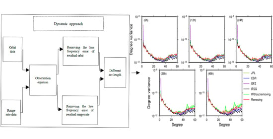
3. The Low-Frequency Error Processing

We will illustrate whether the low-frequency error of the residual orbit needs to be processed on the recovering gravity field by using simulation and real data processing.

3.1. Simulation

In the simulation, the real position and velocity of GRACE at 00:00 h on January 1 2010 are chosen as the initial position and velocity of the simulation. The first degree and order 60 of EGM08 and GIF48 are selected as the real gravity field and reference gravity fields, respectively. The difference between the EOT11A and FES2004 tide model is used as the perturbation model error. In addition, we also assume that there is a deviation of 3 cm and 0.05 cm/s in the initial position and velocity, respectively. Furthermore, there are 2 cm and 1.0 × 10 7 m / s random errors in the orbit and range rate, respectively. The arc lengths of the recovered gravity field are 6, 12, 24, and 48 h respectively. The running time of the satellite is 30 days. The green line expresses the low-frequency error is removed and the magenta line expresses the low-frequency error is not removed. The degree variance and the logarithm of the formal errors are calculated according to Appendix A and Appendix B, respectively. In the inverted triangles, the first row indicates that the low-frequency error of the residual orbit is not removed, while the second row is removed.
The orbit data are used to recover the gravity field. The degree variance of the recovered gravity field for different arc lengths is shown in Figure 1. The accuracy of the gravity field model can be improved by removing the low-frequency error of the residual orbit, that is, the green line is slightly lower than the magenta line. For different arc lengths, the degree and order of the recovered gravity field model orbit is about 45, without removing the low-frequency error of the residual, while the degree and order is about 50 by processing the low-frequency error of the residual orbit. The logarithm of the formal errors of the recovered spherical harmonic coefficient in the form of inverted triangle plots are shown in Figure 2 for different arc lengths. It can be seen that the accuracy can be improved in the second row compared with the first row.
We present the results for the different arc lengths by using the range rate data to recover the gravity field. In Figure 3, the accuracy of the recovered gravity field by removing the low-frequency error is better than the one that does not remove the low-frequency error. The gravity field models are presented by inverted triangles as shown in Figure 4. Compared with the first row, the accuracy of the low-order part of each degree of the recovered gravity field, especially within the order 15, is mainly improved in the second row, and there are obvious blue band areas.
Combine the orbit data and the range rate data to recover the gravity field, where the low-frequency error of the residual range rate is removed. The degree of variance of the recovered gravity field for different arc lengths is shown in Figure 5. Whether or not the low-frequency error of the residual orbit is removed, the accuracy of the first degree and order 50 of the recovered gravity field is basically the same, at 6, 12, and 24 h arcs. But after the degree and order 50, the accuracy of the recovered gravity field by removing the low-frequency error of the residual orbit is better. For 48 h arcs, we can see that the large jump appears around the 30th degree when the low-frequency of the residual orbit is not removed. However, the large jump does not appear when removing the low-frequency error of the residual orbit.
The degree variance of the recovered gravity field for different arc lengths in Figure 5 is plotted in Figure 6 according to whether or not we are processing the low-frequency error of the residual orbit. It can be seen that the degree of variance of the gravity field obtained by removing the low-frequency error of the residual orbit has a good consistency. However, the recovered gravity field without processing the low-frequency error of residual orbit has a good consistency at 6, 12 and 24 h arcs, while the degree variance has a large jump at 48 h arcs, which cannot maintain a good consistency.
The logarithm of the formal errors of the recovered spherical harmonic coefficient for different arc lengths in the form of inverted triangle plots are shown in Figure 7. It can be seen that the accuracy of the multiples of the order 15 of the recovered gravity field and the low order (within the order 15) can be improved. There are obvious blue band areas in the second row of inverted triangles, while the first row does not show such blue bands. In addition, the accuracy of higher-order parts is also improved, just as the red areas on both sides of the inverted triangle are reduced.
In the case of combining the orbit and the range rate to recover gravity field, when removing the low-frequency error of the residual orbit, the advantage of the low-frequency error processing of the residual range rate in Figure 4 is retained in Figure 7, that is, the same blue band region is displayed in the second row of Figure 7. However, this advantage cannot be retained when only the low-frequency error of the residual rate is removed.
From the simulation, we proved that this method can be used to recover the gravity field, the accuracy of the recovered gravity field can be improved, especially the accuracy of the multiples of the order 15, and the accuracy of the recovered gravity field has a good consistency for different arc lengths.

3.2. Real Data Processing

3.2.1. Background Model

According to Formulas (5) and (7), the observation equations of the residual orbit and the residual range rate are established to recover the time-variable gravity field. The reference orbit is required to remove the time-variable signal caused by the N-body perturbations (International Earth Rotation Service (IERS) 2010 conventions), the solid tides (IERS 2010 conventions), the ocean tides (EOT11a, Nmax = 100), the solid earth pole tides (IERS 2010 conventions, C21&S21), the ocean pole tides (Desai model, Nmax = 100), the atmosphere and oceanic variability (AOD1B RL06, Nmax = 180), and the general relativistic perturbations (IERS 2010 conventions). The background field model selected for this purpose is shown in Table 1. In order to reduce the high-frequency signal noise, the first degree and order 180 of the GGM05C model [50] is selected as the static gravity field model. The degree and order of the recovered time-variable gravity field model is 60.

3.2.2. Different Arc Length Processing

GRACE Level-1b data is processed and released by JPL, and the released version is from RL01 to RL03, where every new inversion of GRACE Level-1b data consistently brought clear improvements to gravity field estimates [51]. The latest version currently released is RL03, which improves the quality of the star camera and range rate data comparing with RL02 [52]. Accelerometer calibration is involved in the GRACE data processing. For the accelerometer calibration, we chose to calibrate the hourly biases [11,53]. The process of the recovered time-variable gravity field model is as follows. Firstly, the accelerometer parameters are calibrated according to the existing static gravity field model. Then, we recalculated the reference orbit based on the calibrated accelerometer parameters, and constructed the observation equations of the residual orbit and residual range rate. Finally, we recovered the time-variable gravity field by using the least-squares [20].
In order to ensure that there was enough data to establish the observation equations when the longer arc length is used to recover the time-variable gravity field model, we choose the GRACE data of January 2010 which has fewer discontinuities to recover time-variable gravity fields by using 6, 12, 24, 36, and 48 h arcs, respectively. We present the results according to processing the low-frequency error of the residual range rate or not, where the low-frequency error of the residual range rate is removed. In addition, we select the RL06 model released by CSR, GFZ and JPL, and ITSG-2018 model for comparison. The degree variance of the recovered time-variable gravity field is shown in Figure 8.
In Figure 8, whether or not the low-frequency error of the residual orbit is removed, the accuracy of the recovered time-variable gravity field by using 6, 12 and 24 h arcs is basically the same. However, the difference of the degree variance of the recovered time-variable gravity field gradually increases after 36 h arcs. When removing the low-frequency error of the residual orbit, it can be seen that the degree variance of the recovered time-variable gravity field for different arc lengths has a good consistency with CSR, JPL, GFZ and ITSG-2018.

4. The Monthly Time-Variable Gravity Field Analysis

According to the above simulation, the accuracy of the recovered gravity field can be improved, especially the accuracy of the multiples of the order 15. From the real data processing, the accuracy of the recovered time-variable gravity field models can maintain a good consistency for different arc lengths. In order to further evaluate the performance of solutions derived utilizing this method to consider low-frequency errors, we solved the monthly gravity field model from the periods January 2005 to February 2010, and compared them with the official agencies in terms of the annual amplitude of the mass change and the time series of the characteristics of typical basins. Due to the gaps in the GRACE data and in order to ensure that there are enough data to recover time-variable gravity fields [14], it is not guaranteed to use 48 h arcs to recover time-variable gravity field. Therefore, we used a shorter arc length to recover the time-variable gravity field in some months. According to the statistics, about 35% of the time-variable gravity field is used over 24 h arcs (where 30% is 48 h arcs and 5% is 36 h arcs), about 46% uses 24 h arcs, and about 19% uses less than 24 h arcs (where 6% is 6 h arcs and 13% is 12 h arcs). Because the time-variable gravity field models have exceeded the degree and order 60 provided by CSR, JPL, and GFZ, they are truncated to the degree and order 60 in order to ensure a fair comparison. To get the global mass changes, the post-process of time-variable gravity, including: (1) the C20 is replaced by the result of SLR [54]; (2) the effect of north-south stripes is processed proposed by Swenson and Wahr [55]; (3) the high-frequency noise is filtered by Gaussian smoothing with a radius of 300km; (4) the spherical harmonic coefficients are converted into a global mass changes equivalent water height [56].
In Figure 9, we show the annual amplitudes of the global mass changes from UCAS_IGG, CSR, GFZ, and JPL, respectively. From the spatial distribution, similar large amplitudes are shown, such as in the Amazon basin, central Africa, Tibet Plateau, and north Australia. The correlation coefficients of the mean annual amplitudes of the global mass change among UCAS_IGG and CSR, GFZ, JPL is 0.9942, 0.9933, and 0.9940, respectively.
For further comparisons, we chose the Amazon Basin, Yangtze Basin, Greenland, and Sahara Desert as the study areas [57,58]. The time series are shown in Figure 10, the UCAS_IGG has a good agreement with other models. The correlation coefficients between UCAS_IGG and CSR, GFZ, JPL are shown in Table 2. The correlation coefficients are roughly above 0.9 in the Yangtze River Basin, Greenland, and the Amazon Basin. In Sahara Desert, the standard deviations are 1.58 cm, 1.48 cm, 1.51 cm, and 1.54 cm, respectively. The four institutions are basically at the same level.

5. Discussion

In this study, we analyzed the influence of the low-frequency error of the residual orbit on recovering the time-varying gravity field model by the dynamic approach. According to the results of simulation and real data processing, removing the low-frequency error of the residual orbit or not is related to the arc length used. For the long arc length (such as 48 h arcs), there would be less variables in the initial state when establishing the observation equations, which made the solutions of the observation equations easier. Besides, the method of using the longer arc length could minimize the influence of random errors and means that some small force can be captured [59]. Due to the errors existing in the background model, there are low-frequency errors in the residual orbit and the residual range rate [30,39], which are usually neglected for the shorter arc length. However, this should be modeled for the longer arc length, such as an arc length of more than 24 h. In fact, the low-frequency terms of the residual orbit generated by the time-varying signal and perturbation model error are the same according to formulas (2)–(3), thus it is difficult to separate the perturbation model error and the time-varying signal from the low-frequency part of the residual orbit (within 2CPR) [30,60]. The low-frequency error removing method proposed in this paper not only removes the influence of the perturbation model errors, but also removes the influence of the time-varying signals. However, this method is feasible in terms of the accuracy of the existing background field model, and the arc length of the recovered time-varying gravity field can be prolonged and the time-varying signal can be accurately obtained. In the future, we will need to focus on evaluating the relationship between the accuracy of the background model and the low-frequency error removal method.

6. Conclusions

Based on the orbital perturbation differential equation, we deduced the observation equations of the residual orbit and the residual range rate with the non-linear corrections, respectively. The general solution of the Hill Equation is solved by neglecting the influence of the magnitude of the J 2 term in the satellite moving coordinate system. Under the condition of the perturbation model error and the instrument noise that includes a constant term and 1CPR term, the low-frequency error of the residual orbit is derived in the satellite moving coordinate system. Then, the low-frequency error of the residual range rate is also derived according to the low-frequency error of the residual orbit. There are resonance terms in the low-frequency error formulas of the residual orbit and the residual range rate. As the arc length increases, these resonance terms rapidly enlarge, and thus affect the accuracy of the recovered time-variable gravity field, especially the accuracy of the multiples of the order 15. We recommend that the low-frequency error processing of the residual orbit and residual range rate should both be taken into consideration on recovering time-variable gravity field, especially for the longer arc length.
We use the simulation and real data processing to explain the influence of the low-frequency error of the residual orbit. In the simulation, the accuracy of the recovered gravity field can be improved by removing the low-frequency error, whether only the orbit data or combined orbit data and range rate data are used. In the real data processing, the time-variable gravity field models are recovered by using 6, 12, 24, 36, and 48 h arcs respectively based on January 2010 GRACE data. The accuracy of the recovered time-variable gravity field models by removing the low-frequency error of the residual orbit can always maintain a good consistency for different arc lengths.
We developed the time-variable gravity field model UCAS_IGG from January 2005 to February 2010 by removing the low-frequency error of the residual orbit and the residual range rate. By comparing the mean amplitudes of the global mass changes and the time series of the characteristics of the basin, our recovered time-variable signal levels have a good consistency with the international agencies.

Author Contributions

J.Y., L.L. designed the research; L.L. performed the research, analyzed the data and wrote the paper; M.Z., C.W. revised the paper; L.L., J.Y., C.W., M.Z., W.F., X.W., W.C., and Y.Y. reviewed and edited the writing. All authors have read and agreed to the published version of the manuscript.

Funding

This work is funded jointly by the Major Research Plan of China (No. 2016YFB0501702), the National Nature Science Foundation of China (41774089; 41704013; 42004073), Funded by State Key Laboratory of Geo-Information Engineering (No. SKLGIE2019-M-1-2), the Open Research Fund of Qian Xuesen Laboratory of Space Technology, CAST (No. GZZKFJJ2020006) and the Strategic Priority Research Program of the Chinese Academy of Sciences (No. XDA15017700).

Data Availability Statement

The GRACE Level-1B data are publicly available from the ftp size: ftp://isdcftp.gfz-potsdam.de/grace/Level-1B (accessed on 4 February 2021). The static gravity field models (EGM96, EGM08, and GGM05C) and monthly gravity field solutions (CSR RL06, GFZ RL06, JPL RL06, ITSG-2018, and Tongji-GRACE02) are publicly available from the International Center for Global Earth Model website: http://icgem.gfz-potsdam.de/tom_longtime (accessed on 4 February 2021). The monthly solutions UCAS-IGG are available from the corresponding author upon request.

Conflicts of Interest

The authors declare no conflict of interest.

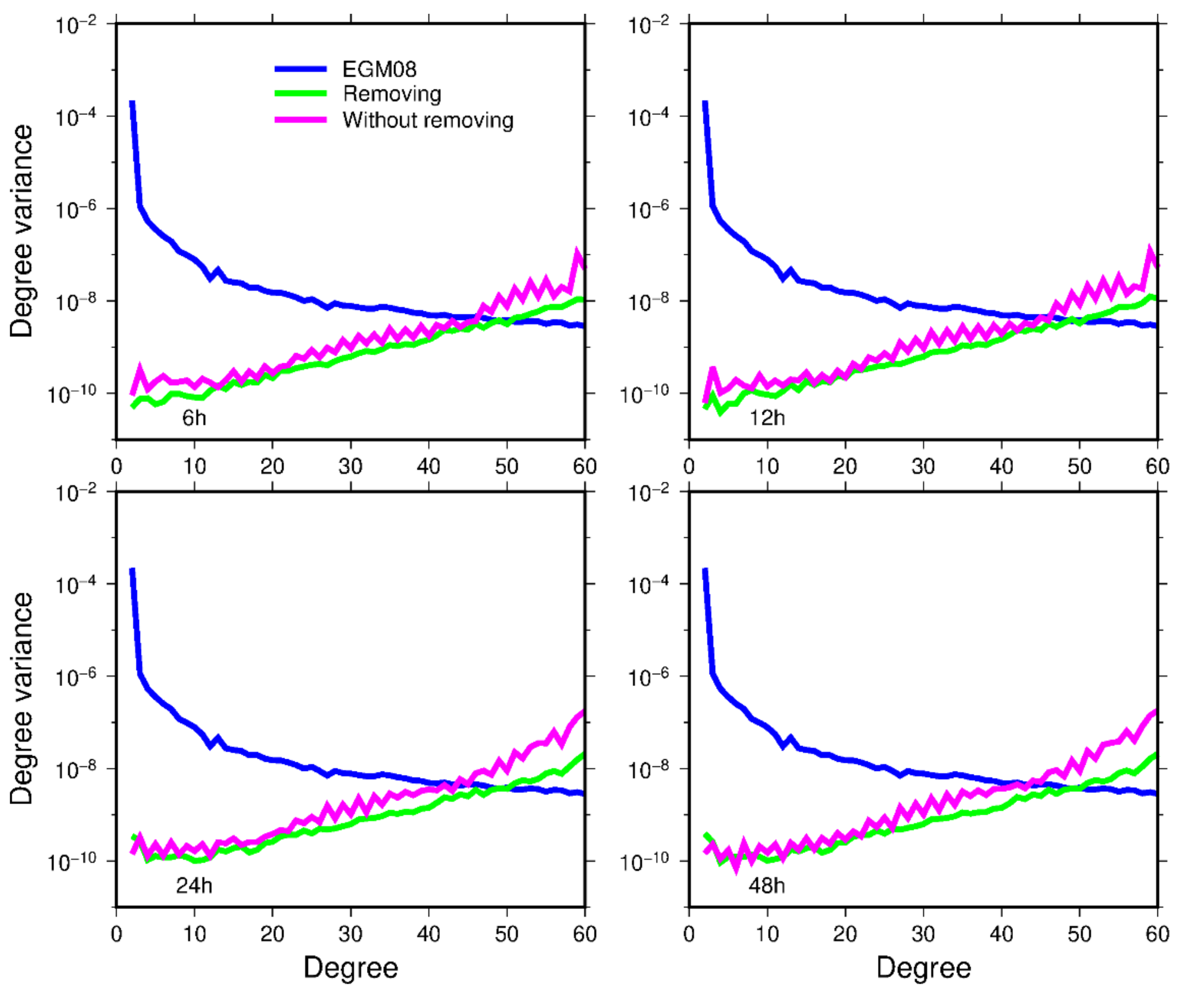
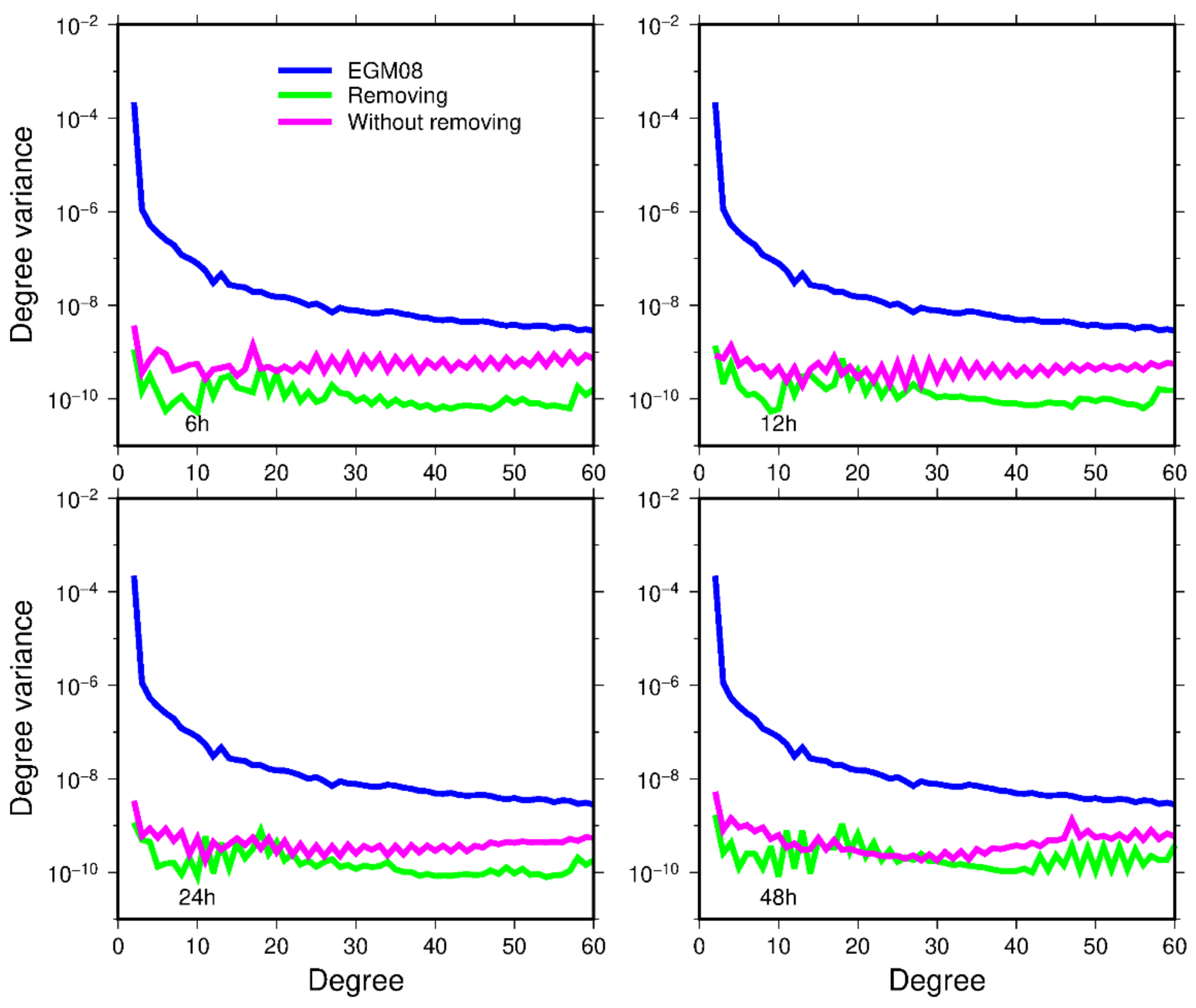
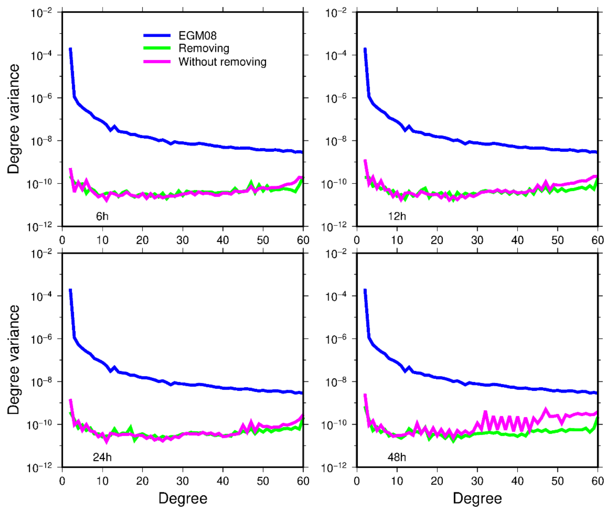
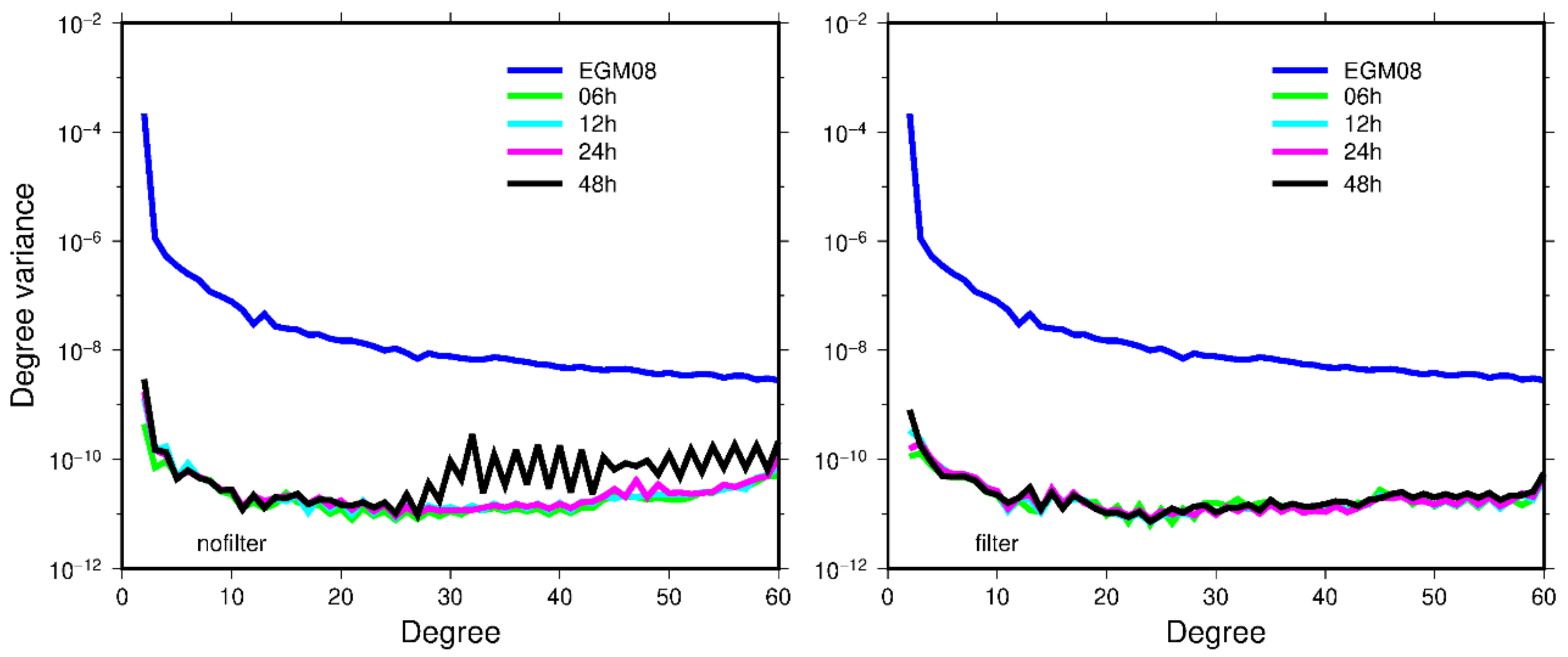
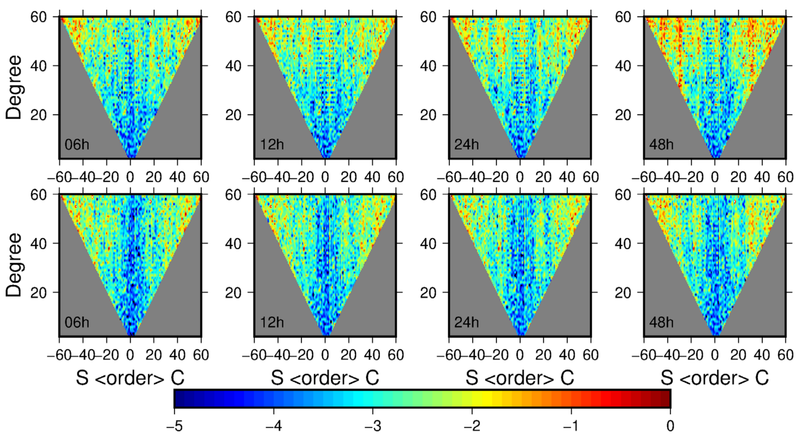
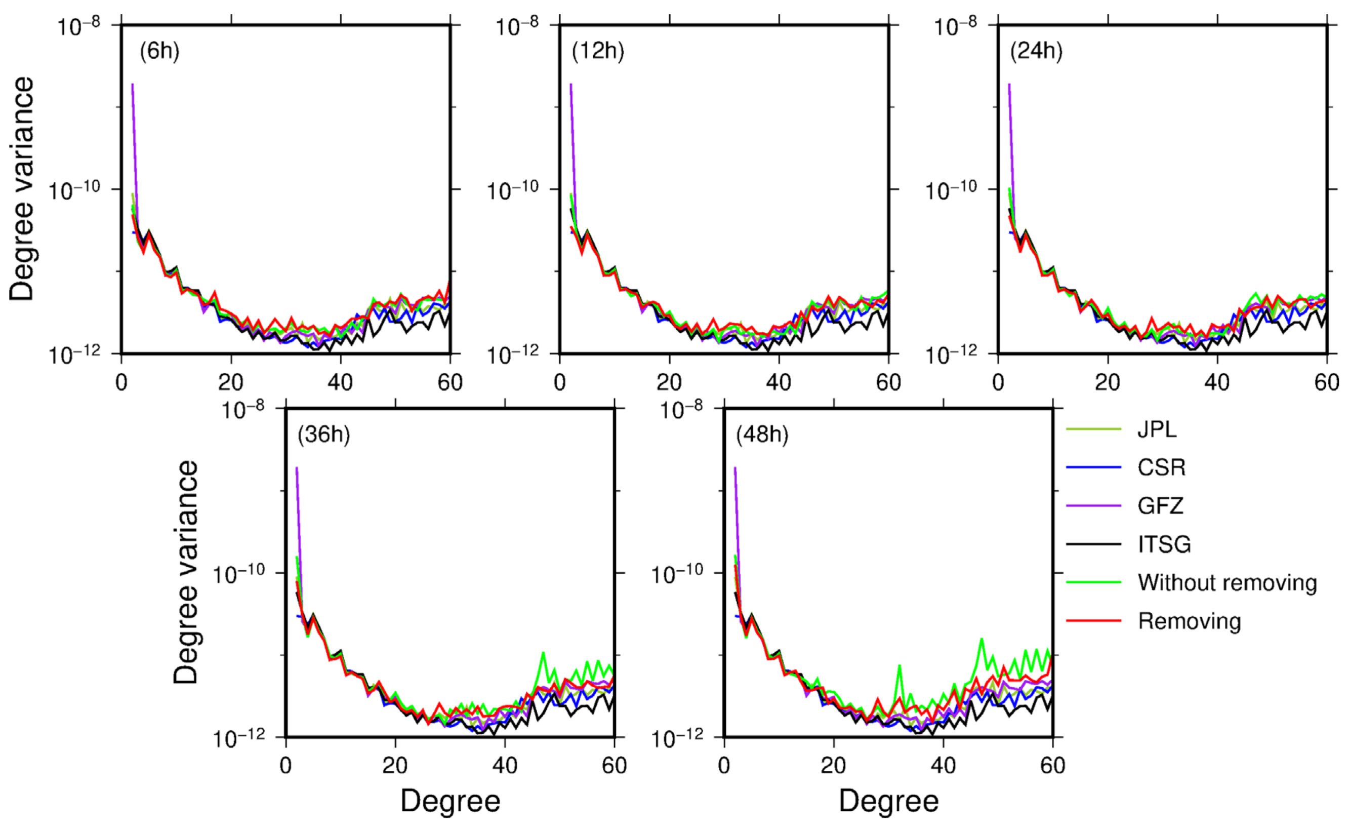
Appendix A. Degree Variance

The n-th degree variance defined by the coefficients of the reference field and estimated gravity field is
Δ n = m = 0 n Δ C ¯ n m 2 + Δ S ¯ n m 2
where
Δ C ¯ n m = C ¯ n m e s t i m a t e C ¯ n m r e f e r e n c e Δ S ¯ n m = S ¯ n m e s t i m a t e S ¯ n m r e f e r e n c e
The subscripts n and m represent the degree and order of the gravity field model, respectively.

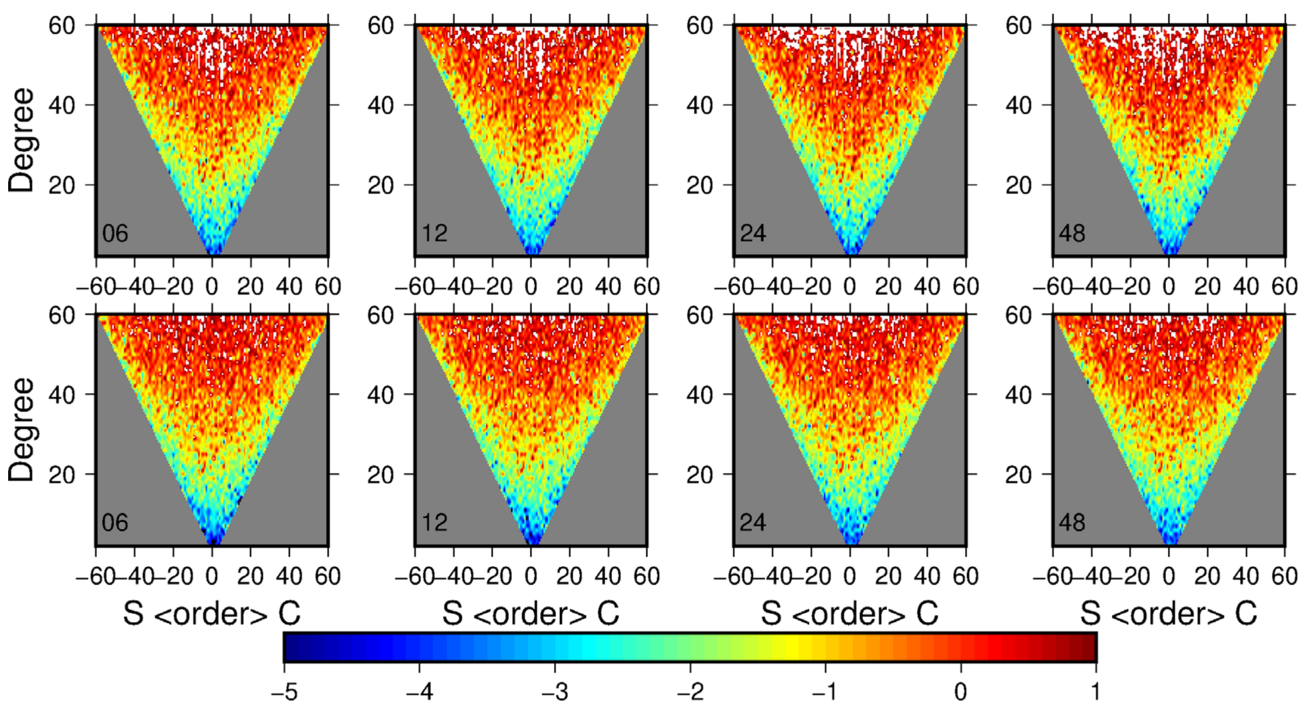
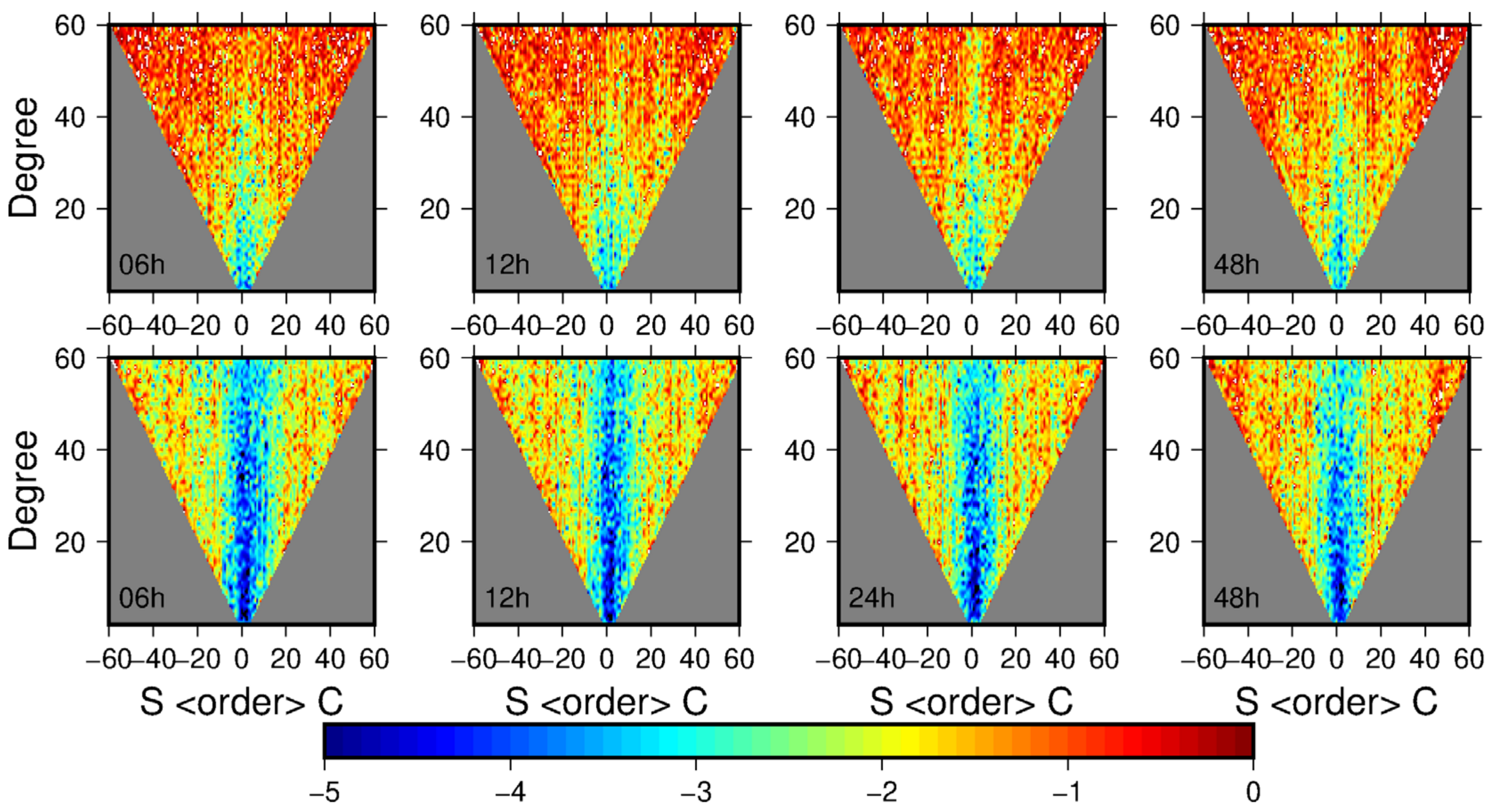
Appendix B. The Logarithm of Formal Errors

The logarithm of formal errors defined by the coefficients of the reference field and the estimated gravity field is
e r r o r n m = lg C ¯ n m e s t i m a t e C ¯ n m r e f e r e n c e C ¯ n m r e f e r e n c e , m 0 lg S ¯ n m e s t i m a t e S ¯ n m r e f e r e n c e S ¯ n m r e f e r e n c e , m < 0
The subscripts n and m represent the degree and order of the gravity field model, respectively.

References

  1. Tapley, B.D.; Bettadpur, S.; Ries, J.C.; Thompson, P.F.; Watkins, M.M. GRACE measurements of mass variability in the Earth system. Science 2004, 305, 503–505. [Google Scholar] [CrossRef] [PubMed] [Green Version]
  2. Tapley, B.D.; Bettadpur, S.; Watkins, M.; Reigber, C. The gravity recovery and climate experiment: Mission overview and early results. Geophys. Res. Lett. 2004, 31, L09607. [Google Scholar] [CrossRef] [Green Version]
  3. Tapley, B.D.; Ries, J.; Bettadpur, S.; Chambers, D.; Cheng, M.; Condi, F.; Gunter, B.; Kang, Z.; Nagel, P.; Pastor, R.; et al. GGM02- an improved earth gravity field model from GRACE. J. Geod. 2005, 79, 467–478. [Google Scholar] [CrossRef]
  4. Bettadpur, S. Gravity Recovery and Climate Experiment UTCSR Level-2 Processing Standards Document for Level-2 Product Release 005. Available online: https://www.researchgate.net/publication/289630299_UTCSR_Level-2_Processing_Standards_Document_for_Level-2_Product_Release_0005_Center_for_Space_Research_Technical_Report_GRACE (accessed on 4 February 2021).
  5. Dahle, C.; Flechtner, F.; Gruber, C.; König, D.; König, R.; Michalak, G.; Neumayer, K.H. GFZ GRACE level-2 processing standards document for level-2 product release 0005. Sci. Tech. Rep. Data 2012, 12, 1–21. [Google Scholar]
  6. Save, H.; Bettadpur, S.; Tapley, B.D. High-resolution CSR GRACE RL05 mascons. J. Geophys. Res. Solid Earth 2016, 121, 7547–7569. [Google Scholar] [CrossRef]
  7. Watkins, M.M.; Wiese, D.; Yuan, D.N.; Boening, C.; Landerer, F.W. Improving methods for observing Earth’s time variable mass distribution with GRCE using spherical cap mascons. J. Geophys. Res. Solid Earth 2015, 120, 2648–2671. [Google Scholar] [CrossRef]
  8. Zhou, H.; Luo, Z.C.; Zhou, Z.B.; Li, Q.; Zhong, B.; Lu, B.; Hsu, H.Z. Impact of different kinematic empirical parameters processing strategies on temporal gravity field model determination. J. Geophys. Res. Solid Earth 2018, 123, 1–25. [Google Scholar] [CrossRef]
  9. Guo, X.; Zhao, Q.L.; Ditmar, P.; Sun, Y.; Liu, J.N. Improvements in the monthly gravity field solutions through modeling the colored noise in the GRACE data. J. Geophys. Res. Solid Earth 2018, 123, 7040–7054. [Google Scholar] [CrossRef]
  10. Liang, L.; Yu, J.H.; Zhu, Y.C.; Wan, X.Y.; Chang, L.; Huan, X.; Wang, K. Recovered GRACE time-variable gravity field based on dynamic approach with the non-linear corrections. Chin. J. Geophys. 2019, 62, 3259–3268. (In Chinese) [Google Scholar]
  11. Mayer-Gürr, T. Gravitationsfeldbestimmung aus der Analyse kurzer Bahnbögen am Beispielder Satellitenmissionen CHAMP und GRACE; University of Bonn: Bonn, Germany, 2006. [Google Scholar]
  12. Kurtenbach, E.; Mayer-Gürr, T.; Eicker, A. Deriving daily snapshots of the Earth’s gravity field from GRACE L1B data using Kalman filtering. Geophys. Res. Lett. 2009, 36, L17102. [Google Scholar] [CrossRef]
  13. Chen, Q.J.; Shen, Y.Z.; Chen, W.; Zhang, X.F.; Hsu, H.Z. An improved GRACE monthly gravity field solution by modeling the non-conservative acceleration and attitude observation errors. J. Geod. 2016, 90, 503–523. [Google Scholar] [CrossRef]
  14. Chen, Q.J.; Shen, Y.Z.; Olivier, F.; Chen, W.; Zhang, X.F.; Hsu, H.Z. Tongji-Grace02s and Tongji-Grace02k: High-precision static GRACE-only global Earth’s gravity field models derived by refined data processing strategies. J. Geophys. Res. Solid Earth 2018, 123, 6111–6137. [Google Scholar] [CrossRef]
  15. Chen, Q.J.; Shen, Y.Z.; Chen, W.; Olivier, F.; Zhang, X.F.; Chen, Q.; Li, W.W.; Chen, T.Y. An optimized short-arc approach: Methodology and application to develop refined time series of Tongji-Grace2018 GRACE monthly solutions. J. Geophys. Res. Solid Earth 2019, 124, 6010–6038. [Google Scholar] [CrossRef]
  16. Ditmar, P.; Sluijs, A.A.V.E.V.D. A technique for modeling the Earth’s gravity field on the basis of satellite accelerations. J. Geod. 2004, 78, 12–33. [Google Scholar] [CrossRef]
  17. Ditmar, P.; Kuznetsov, V.; van der Sluijs, A.V.A.; Schrama, E.; Klees, R. ‘DEOS_CHAMP-01C_70’: A model of the Earth’s gravity field computed from accelerations of the CHAMP satellite. J. Geod. 2006, 79, 586–601. [Google Scholar] [CrossRef] [Green Version]
  18. Liu, X. Global Gravity Field Recovery from Satellite-to-Satellite Tracking Data with the Acceleration Approach; Delft University of Technology: Delft, The Netherlands, 2008. [Google Scholar]
  19. Liu, X.; Ditmar, P.; Siemes, C.; Slobbe, D.C.; Revtova, E.; Klees, R.; Riva, R.; Zhao, Q. DEOS Mass Transport model (DMT-1) based on GRACE satellite data: Methodology and validation. Geophys. J. Int. 2010, 181, 769–788. [Google Scholar] [CrossRef] [Green Version]
  20. Beutler, G.; Jäggi, A.; Mervart, L.; Meyer, U. The celestial mechanics approach: Theoretical foundations. J. Geod. 2010, 84, 605–624. [Google Scholar] [CrossRef] [Green Version]
  21. Beutler, G.; Jäggi, A.; Mervart, L.; Meyer, U. The celestial mechanics approach: Application to data of the GRACE mission. J. Geod. 2010, 84, 661–681. [Google Scholar] [CrossRef] [Green Version]
  22. Jekeli, C. The determination of gravitational potential differences from satellite-to-satellite tracking. Celest. Mech. Dyn. Astron. 1999, 75, 85–100. [Google Scholar] [CrossRef]
  23. Han, S.C.; Shum, C.K.; Jekeli, C. Precise estimation of in situ geopotential differences from GRACE low-low satellite-to-satellite tracking and accelerometer data. J. Geophys. Res. 2006, 111, B04411. [Google Scholar] [CrossRef] [Green Version]
  24. Ramillien, G.; Biancale, R.; Gratton, S.; Vasseur, X.; Bourgogne, S. GRACE-derived surface water mass anomalies by energy integral approach: Application to continental hydrology. J. Geod. 2011, 6, 313–328. [Google Scholar] [CrossRef]
  25. Tangdamrongsub, N.; Hwang, C.; Wang, L. Regional surface mass anomalies from GRACE KBR measurements: Application of L-curve reqularinzation and a priori hydrological knowledge. J. Geophys. Res. 2012, 117, B11406. [Google Scholar]
  26. Zeng, Y.Y.; Guo, J.Y.; Shang, K.; Shum, C.K.; Yu, J.H. On the formulation of gravitational potential difference between the GRACE satellites based on energy integral in earth fixed frame. Geophys. J. Int. 2015, 202, 1792–1804. [Google Scholar] [CrossRef]
  27. Shang, K.; Guo, J.Y.; Shum, C.K.; Dai, C.L.; Luo, J. GRACE time-variable gravity field recovery using an improved energy balance approach. Geophys. J. Int. 2015, 203, 1773–2786. [Google Scholar] [CrossRef]
  28. Watkins, M.M.; Yuan, D.N. GRACE JPL Level-2 Processing Standards Document for Level-2 Product Release 05; GRACE 327-744(v 5.0); 2012; Available online: ftp://isdcftp.gfz-posdam.de/grace/ (accessed on 4 February 2021).
  29. Kim, J. Simulation Study of a Low-Low Satellite-to-Satellite Tracking Mission; The University of Texas at Austin: Austin, TX, USA, 2000. [Google Scholar]
  30. Zhao, Q.L.; Guo, J.; Hu, Z.G.; Shi, C.; Liu, J.N.; Cai, H.; Liu, X.L. GRACE gravity field modeling with an investigation on correlation between nuisance parameters and gravity field coefficients. Adv. Space Res. 2011, 47, 1833–1850. [Google Scholar] [CrossRef]
  31. Visser, P. Low-low satellite-to-satellite tracking: A comparison between analytical linear orbit perturbation theory and numerical integration. J. Geod. 2005, 79, 160–166. [Google Scholar] [CrossRef]
  32. Bruinsma, S.; Lemoine, J.M.; Biancale, R.; Valeś, N. CNES/GRGS 10-day gravity field models (release 2) and their evaluation. Adv. Space Res. 2010, 45, 587–601. [Google Scholar] [CrossRef]
  33. Meyer, U.; Jäggi, A.; Beutler, G. Monthly gravity field solutions based on GRACE observations generated with the Celestial Mechanics Approach. Earth Planet Sci. Lett. 2012, 345–348, 72–80. [Google Scholar] [CrossRef]
  34. Ditmar, P.; da Encarnação, J.T.; Farahani, F.F. Understanding data noise in gravity field recovery on the basis of inter-satellite ranging measurements acquired by the satellite gravimetry mission GRACE. J. Geod. 2012, 86, 441–465. [Google Scholar] [CrossRef] [Green Version]
  35. Hashemi Farahani, H.; Ditmar, P.; Klees, R.; Liu, X.; Zhao, Q.; Guo, J. The static gravity field model DGM-1S from GRACE and GOCE data: Computation, validation and an analysis of GOCE mission’s added value. J. Geod. 2013, 87, 843–867. [Google Scholar] [CrossRef]
  36. Wang, C.Q.; Xu, H.Z.; Zhong, M.; Feng, W.; Ran, J.J.; Yang, F. An investigation on GRACE temporal gravity field recovery using the dynamic approach. Chin. J. Geophys. 2015, 58, 756–766. (In Chinese) [Google Scholar]
  37. Luo, Z.C.; Zhou, H.; Li, Q.; Zhong, B. A new-time-variable gravity field model recovered by dynamic integral approach on the basis of GRACE KBRR data alone. Chin. J. Geophys. 2015, 59, 1994–2005. (In Chinese) [Google Scholar]
  38. Colombo, O.L. The Global Mapping of Gravity with Two Satellite; Publications on Geodesy, New Series; Netherlands Geodetic Commission: Delft, Switzerland, 1984. [Google Scholar]
  39. Seo, K.W.; Wilson, C.R.; Chen, J.L.; Waliser, D.E. GRACE’s spatial aliasing error. Geophys. J. Int. 2008, 172, 41–48. [Google Scholar] [CrossRef] [Green Version]
  40. Kaula, W.M. Theory of Satellite Geodesy: Applications of Satellites to Geodesy; Blaisdell: Waltham, MA, USA, 1966. [Google Scholar]
  41. Montenbruck, O.; Gill, E. Satellite Orbits; Springer: Berlin/Heidelberg, Germany, 2000. [Google Scholar]
  42. Reigber, C. Gravity field recovery from satellite tracking data. In Theory of Satellite Geodesy and Gravity Field Determination—Lecture Notes in Earth Sciences; Sansό, F., Rummel, R., Eds.; Springer: Berlin/Heidelberg, Germany, 1989; pp. 197–234. [Google Scholar]
  43. Tapley, B.D. Fundamentals of orbit determination. In Theory of Satellite Geodesy and Gravity Field Determination—Lecture notes in Earth Sciences; Sansό, F., Rummel, R., Eds.; Springer: Berlin/Heidelberg, Germany, 1989; pp. 235–260. [Google Scholar]
  44. Yu, J.H.; Zhu, Y.C.; Meng, X.C. Orbital perturbation differential equations with non-linear corrections for Champ-like satellite. Chin. J. Geophy. 2017, 60, 286–299. [Google Scholar]
  45. Xu, P. Position and velocity perturbations for the determination of geopotential from space geodetic measurements. Celest. Mech. Dyn. Astron. 2008, 100, 231–249. [Google Scholar] [CrossRef]
  46. Heiskanen, W.A.; Moritz, H. Physical Geodesy; Freeman, W.H. and company: San Fracisco, CA, USA, 1967; pp. 1–32. [Google Scholar]
  47. Petit, G.; Luzum, B. IERS Conventions; Bonifatius GmbH: Paderborn, Germany, 2010. [Google Scholar]
  48. Kaplan, M.H. Modern Spacecraft Dynamics & Control; Wiley: New York, NY, USA, 1976. [Google Scholar]
  49. McCullough, G.M. Gravity Field Estimation for Next Generation Satellite Missions; University of Texas at Austin: Austin, TX, USA, 2007. [Google Scholar]
  50. Ries, J.; Bettadpur, S.; Eanes, R.; Kang, Z.; Ko, U.; McCullough, C.; Nagel, P.; Pie, N.; Poole, S.; Richter, T.; et al. The Combination Global Gravity Model GGM05C; The University of Texas at Austin: Austin, TX, USA, 2016. [Google Scholar]
  51. Bandikova, T.; Flury, J. Improvement of the GRACE star camera data based on the revision of the combination method. Adv. Space Res. 2014, 54, 1818–1827. [Google Scholar] [CrossRef]
  52. Bandikova, T. The Role of Attitude Determination for Inter-Satellite Ranging. Ph.D. Thesis, Leibniz University of Hannover, Hannover, Germany, 2015. [Google Scholar]
  53. Chen, Q.J.; Shen, Y.Z.; Zhang, X.F.; Hsu, H.Z.; Chen, W.; Ju, X.L.; Lou, L.Z. Monthly gravity field models derived from GRACE Level 1B data using a modified short-arc approach. J. Geophys. Res. Solid Earth 2015, 120, 1804–1819. [Google Scholar] [CrossRef]
  54. Cheng, M.K.; Tapley, B.D. Variations in the Earth’s oblateness during the past 28 years. J. Geophys. Res. 2004, 109, B09402. [Google Scholar] [CrossRef]
  55. Swenson, S.; Wahr, J. Post-processing removal of correlated errors in GRACE data. Geophys. Res. Lett. 2006, 33, L08402. [Google Scholar] [CrossRef]
  56. Wahr, J.; Swenson, S.; Zlotnicki, V.; Velicogna, I. Time-variable gravity from GRACE: First results. Geophys. Res. Lett. 2004, 31, L11501. [Google Scholar] [CrossRef] [Green Version]
  57. Yang, F.; Wang, C.Q.; Hus, H.Z.; Zhong, M.; Zhou, Z.B. Towards a more accurate temporal gravity model from GRACE observations through the kinematic orbits. Chin. J. Geophys. 2017, 60, 37–49. (In Chinese) [Google Scholar]
  58. Ran, J.J.; Xu, H.Z.; Zhong, M.; Feng, W.; Shen, Y.Z.; Zhang, X.F.; Yi, W.Y. Global temporal gravity field recovery using GRACE data. Chin. J. Geophys. 2014, 57, 1032–1040. (In Chinese) [Google Scholar]
  59. Shen, Y.Z. Algorithm characteristics of dynamic approach-based satellite gravimetry and its improvement proposals. Acta Geod. Cartogr. Sin. 2017, 46, 1308–1315. [Google Scholar]
  60. Ray, R.D.; Luthcke, S.B. Tide model errors and GRACE gravimetry: Towards a more realistic assessment. Geophys. J. Int. 2006, 167, 1055–1059. [Google Scholar] [CrossRef] [Green Version]
Figure 1. The degree variance of the recovered gravity field by using 6, 12, 24, and 48 h arcs, when using orbit data to recover gravity field.
Remotesensing 13 01118 g001
Figure 2. The logarithm of formal errors (comparing the EGM08) in the spherical harmonic coefficients of the recovered gravity field by using 6, 12, 24, and 48 h arcs, when using the orbit data to recover the gravity field.
Remotesensing 13 01118 g002
Figure 3. The degree variance of the recovery gravity field by using 6, 12, 24 and 48 h arcs, when using the range rate data to recover the gravity field.
Remotesensing 13 01118 g003
Figure 4. The logarithm of formal errors (comparing the EGM08) in the spherical harmonic coefficients of the recovered gravity field by using 6, 12, 24, and 48 h arcs, when using the range rate data to recover gravity field.
Remotesensing 13 01118 g004
Figure 5. The degree variance of the recovered gravity field by using 6, 12, 24 and 48 h arcs, when combining the orbit data and the range rate data to recover the gravity field.
Remotesensing 13 01118 g005
Figure 6. The degree variance of the recovered gravity field by using 6, 12, 24, and 48 h arcs, respectively. (The left expresses do not process the low-frequency error of residual orbit; the right expresses the process of the low-frequency error of residual orbit.).
Remotesensing 13 01118 g006
Figure 7. The logarithm of formal errors (comparing the EGM08) in the spherical harmonic coefficients of the recovered gravity field by using 6, 12, 24, and 48 h arcs, when combining the orbit and range rate to recover the gravity field.
Remotesensing 13 01118 g007
Figure 8. The degree variance of the recovered time-variable gravity field model based on the GRACE data of Jan. 2010.
Remotesensing 13 01118 g008
Figure 9. Annual amplitude of global mass change from January 2005 to February 2010 by different time-variable gravity field models (equivalent water height, unit: cm). (a) UCAS_IGG; (b) CSR; (c) GFZ; (d) JPL.
Remotesensing 13 01118 g009
Figure 10. From January 2005 to February 2010, time series of land water changes based on the time-variable gravity field model in (a) Sahara Desert, (b) Yangtze River Basin, (c) Greenland Island, and (d)Amazon Basin (Equivalent water height, unit: cm) based on the different time-variable gravity field models.
Remotesensing 13 01118 g010
Table 1. Perturbation model.
Force ModelDescription
Static gravity field modelGGM05C(180*180)
N-body perturbationJPL DE421
Solid Earth tidesIERS 2010 Conventions
Solid Earth pole tidesIERS mean pole
Ocean tidesEOT11a(100*100)
Ocean pole tideDesai model(100*100)
Atmospheric and Oceanic de-aliasingAOD1B RL06(180*180)
General RelativisticIERS 2010 conventions
Non-gravitational forcesOnboard accelerometer data
Table 2. Correlation coefficients between UCAS_IGG and CSR, GFZ, JPL.
Correlation CoefficientsCSRGFZJPL
Sahara desert0.850.800.87
Yangtze River Basin0.990.980.99
Greenland Island0.950.910.96
Amazon Basin0.990.990.99
Publisher’s Note: MDPI stays neutral with regard to jurisdictional claims in published maps and institutional affiliations.

