Article

High-Resolution SMAP-Derived Root-Zone Soil Moisture Using an Exponential Filter Model Calibrated per Land Cover Type

by
Vivien-Georgiana Stefan
1,*,
Gianfranco Indrio
1,
Maria-José Escorihuela
1,
Pere Quintana-Seguí
2 and
Josep Maria Villar
3
1
isardSAT SL, 08042 Barcelona, Spain
2
Observatori de l’Ebre, 43520 Roquetes, Spain
3
Department of Environment and Soil Sciences, Universitat de Lleida, 25198 Lleida, Spain
*
Author to whom correspondence should be addressed.
Remote Sens. 2021, 13(6), 1112; https://doi.org/10.3390/rs13061112
Submission received: 26 January 2021 / Revised: 27 February 2021 / Accepted: 9 March 2021 / Published: 15 March 2021

Abstract

:
Root-zone soil moisture (RZSM) plays a key role for most water and energy budgets, as it is particularly relevant in controlling plant transpiration and hydraulic redistribution. RZSM data is needed for a variety of different applications, such as forecasting crop yields, improving flood predictions and monitoring agricultural drought, among others. Remote sensing provides surface soil moisture (SSM) retrievals, whose key advantage is the large spatial coverage on a systematic basis. This study tests a simple method to retrieve RZSM estimates from high-resolution SSM derived from SMAP (Soil Moisture Active Passive). A recursive exponential filter using a time constant τ is calibrated per land cover type, which uses as an intermediate step a long-term ISBA-DIF (Interaction Soil Biosphere Atmosphere—Diffusion scheme) dataset over an area located in Catalonia, NE of Spain. The τ values thus obtained are then used as an input to the same recursive exponential filter, to derive 1 km resolution RZSM estimates from 1 km SMAP SSM, which are obtained from the original data by downscaling to a 1 km resolution, through the DISPATCH (DISaggregation based on a Physical and Theoretical scale CHange) methodology. The results are then validated with scaled in situ observations at different depths, over two different areas, one representative of rainfed crops, and the other of irrigated crops. In general, the estimates agree well with the observations over the rainfed crops, especially at a 10 cm and 25 cm depth. Nash–Sutcliffe (NS) scores ranging between 0.33 and 0.58, and between 0.37 and 0.56 have been found, respectively. Correlation coefficients for these depths are high, between 0.76 and 0.91 (10 cm), and between 0.71 and 0.90 (25 cm). For the irrigated sites, results are poorer (partly due to the extremely high heterogeneity present), with NS scores ranging between −2.57 and 0.16, and correlations ranging between −0.56 and 0.48 at 25 cm. Given the strong correlations and NS scores found in the surface, the sensitivity of the filter to different τ values was investigated. For the rainfed site, it was found, as expected, with increasing τ , increasing NS and correlations with the deeper layers, suggesting a better coupling. Nevertheless, a strong correlation with the surface (5 cm) or shallower depths (10 cm) observed over certain sites indicates a certain lack of skill of the filter to represent processes which occur at lower levels in the SM column. All in all, a calibration accounting for the vegetation was shown to be an adequate methodology in applying the recursive exponential filter to derive the RZSM estimates over large areas. Nevertheless, the relative shallow surface at which the estimates correlate in some cases seem to indicate that an effect of evapotranspiration in the profile is not well captured by the filter.

1. Introduction

Among existing hydrological variables, soil moisture (SM) is essential to land-atmosphere interactions, through its influence on energy and moisture fluxes in the boundary layer [1,2]. Moreover, it plays a crucial role in the climate system, through its impact on evaporation, infiltration and run-off [3]. SM data are needed at a range of different spatial scales, depending on the application domain. Therefore, climatological and meteorological applications use rather coarse resolution data, hydrological applications are usually focused on the watershed scale, while agricultural applications require high (at least 1 km) data.
With the advent of remote sensing, the past ten years have seen a significant focus given to passive microwave and active sensors to provide spatially distributed SM data on a global level [4,5]. In particular, passive L-band microwave sensors are widely used to derive SM, due to their strong physical link between the brightness temperature and the SM present in the top layer [6,7]. However, the spatial resolution of L-band microwave sensors is coarse (40 – 60 km), which is not enough when it comes to using the data within agricultural applications. On the other hand, the active sensors have the advantage of providing data at high spatial resolutions. Several studies have investigated the potential of using Synthetic Aperture Radar (SAR) data, in particular C-band and L-band, to derive SM products [8,9]. However, difficulties are encountered when taking into account the soil roughness and the vegetation backscattering effects in the SM modeling.
Among the existing satellite missions, there are two dedicated specifically to the measuring of SM: the Soil Moisture and Ocean Salinity (SMOS, [4]), launched by the European Space Agency (ESA) in 2009, and  the Soil Moisture Active Passive (SMAP, [10]), launched by the US National Aeronautics and Space Administration (NASA) in 2015. They both provide surface soil moisture (SSM) observations, characteristic to the first 5 cm of the soil [4], at similar spatial resolutions:  40 km (SMOS), 36 km (SMAP). However, the soil moisture information needed for most energy and water budgets pertains to a deeper layer [11,12,13]. The SM characteristic to this layer is also known as root-zone soil moisture (RZSM) and it is particularly relevant as it controls plant transpiration and hydraulic redistribution [14].
RZSM estimates are particularly important in a range of different applications such as: forecasting agricultural productivity [15], providing better representation of evapotranspiration for climate change projections [16], improving flood predictions [17], assisting in predicting the severity of wildfires [18], and monitoring agricultural drought [19]. An analytical relationship between the SSM and the SM in the lower layers is therefore needed [20].
Remote sensing SSM observations have been assimilated or used as forcing into different land surface models (LSM) and crop models, in order to derive RZSM, with the model errors being partially reduced [21,22,23,24,25,26]. Nevertheless, the studies reported that using SSM alone is limited by the disconnection between surface and subsurface dynamics, which in turn leads to uncertainties in the root-zone model. Estimating RZSM from SSM and integrating it into hydrological models impacts the water and weather forecasting systems [27]. Current techniques of deriving RZSM from SSM include methodologies based on field measurements [28,29,30], satellite observations [31,32,33,34,35] and data assimilation [36,37,38].
Data assimilation methods are widely used, due to their capability of providing RZSM predictions, while accounting for uncertainties between observed data and model outputs [27]. SSM is linked to RZSM through diffusion, which makes it possible to use assimilation algorithms to derive RZSM from SSM data [39,40,41,42,43,44]. Data assimilation has been widely used in recent years to derive RZSM estimates by integrating SSM measurements into land surface models (LSM, [35,45,46,47,48,49]). It is generally regarded that the Ensemble Kalman Filter is well suited for the estimation of profile SM [43], as it is an optimal sequential method that has been extensively used. However, the main drawbacks to the Ensemble Kalman Filter are the strong limitations in the case of nonlinear systems [50], as well as its high computational demands. Overall, data assimilation methods are limited by several factors, including the uncertainties linked to the physical description of the energy and water balance, as well as the lack of high-quality information on the model parameters on a global scale [51]. In addition, the RZSM estimates provided by LSM are model dependent, particularly because the estimation is highly linked to the soil texture and vegetation coverage [41].
Regression approaches are used to bypass the computationally heavy aspect linked with data assimilation within LSM [52]. Ref. [53] have proposed using an ensemble of artificial neural networks for the derivation of RZSM from SSM, based on the notion that the modeled relationship is derived from data, accounting for soil water transmission as well as the impact of surface fluxes in a representative way for the unknown SM interactions.
An exponential filter was proposed [54] to derive the amount of water moving from the surface into the root zone (also referred to as soil water index in the root-zone layer), using satellite SSM observations. The filter takes into consideration an empirically derived parameter, which can be regarded as a “pseudodiffusivity” constant that controls how much of the SSM content infiltrates in the root-zone layer and for how long it stays there, the unit being a period of days. The soil water index is considered instead of actual values of RZSM due to the large variability of the soil characteristics within the satellite footprint, which might not be represented in an accurate manner [51]. Therefore, the relative dynamic range of the soil moisture in the root-zone is instead represented [55]. Several studies applied the methodology to estimate RZSM and validate it with in situ measurements [56,57]. The exponential filter model has been previously used to derive RZSM from satellite SSM observations [51,56,58,59,60], as well as from in situ SSM measurements or modeled SSM [51,61]. An assumption made when using the exponential filter is that there is a hydrologic equilibrium within the soil profile [62], which makes it possible to derive RZSM estimates from SSM observations, provided that soil physical properties are known. This implies a reduced sensitivity over prolonged dry periods, when the plant uptake is the main driving force within RZSM movement [62]. Moreover, RZSM weakens with depth [63] for most soil types, meaning that the sensitivity of the exponential filter weakens at deeper layers [33], which in turn leads to the conclusion that the model provides relatively better results under humid conditions [19,64].
An important thing to keep in mind when applying the exponential filter to derive RZSM data is that the pseudodiffusivity parameter needs to be calibrated. Most studies [33,51,62,65] have calibrated this parameter by using either in situ data, modeled data, or remote sensing data collected over the respective study sites. However, if one is to take advantage of the global coverage of remote sensing data, without the need for site-specific calibration, a global map of the pseudodiffusivity parameter is needed. One possible step into achieving this is by calibrating the pseudodiffusivity parameter per land cover type. Such a calibration is reasonable, given that different land cover types have different root-zone layer depths, and hence might need a different pseudodiffusivity parameter to properly describe the water content at their specific root depth.
One of our study’s main goals is to investigate the potential of such a calibration in deriving reliable RZSM estimates. Another aspect our study aims to investigate is the assessment of the potential this exponential filter has in deriving RZSM at different depths. For example, Refs. [33,51] have implemented the exponential filter and compared the RZSM estimates with in situ measurements at specified depths: 30 and 25 cm, respectively. Our study aims at comparing the RZSM estimates with in situ measurements at different depths, in order to assess the most likely depth at which the filter’s estimates are most representative.
In this respect, the recursive formulation of the exponential filter in [66] is used to derive 1 km RZSM from SMAP data. The recursive formulation is chosen for implementation because it offers the advantage of handling data more easily than the original version. The horizontal discrepancy between the scale at which satellite observations are made and the scale at which natural processes occur within the SM profile is handled by first downscaling the SMAP data using the DISPATCH (DISaggregation based on a Physical and Theoretical scale Change, [67]) methodology. In order to calibrate the pseudodiffusivity parameter associated with the filter per land cover type, an intermediate step is performed, and a value is derived by using ISBA-DIF (Interaction Soil-Atmosphere-Biosphere-Diffusion scheme) SSM and RZSM. These values are then cross-referenced with the land cover type present within the study area, and a general map is obtained by averaging all the parameter values obtained previously that fall within each land cover type. The obtained pseudodiffusivity parameter values are then used to derive 1 km RZSM estimates over two areas in the NE of the Iberian Pensinsula, which are consequently validated against in situ measurements located in rainfed and irrigated crops. The filter is then tested over the same area, with different pseudodiffusivity parameter values, in order to assess its influence on the depth at which the estimates are most representative of.
The article is structured as follows: a description of the study area and datasets used is offered in Section 2, Section 3 explains the methodology behind the exponential filter model and the pseudodiffusivity parameter calibration, while Section 4 offers a presentation of the in situ validation, as well as a study on the influence of the parameter at different depths.

2. Data Description

2.1. Validation Sites and In Situ Data

The study area (40–43 N, 0–4 E) is in the North-East of the Iberian Peninsula, where the approach to derive the 1 km resolution RZSM is applied. For validation purposes, we focus our attention on two regions in particular: the Terres de l’Ebre region and the Algerri Balguer irrigation district, both representative of Mediterranean climate, but with different land-use practices and landforms. Figure 1 is a visual representation of the extended study area, as well as the two validation sites.
The Terres de l’Ebre region presents hot summers and mild winters, with a mean yearly temperature of 24 C in summer and 6 C in winter, and a mean yearly precipitation of 545 mm. The main crops cultivated in the area include rainfed crops (olive trees, vineyards, almond trees), while the main irrigated crops include rice and fruit trees (peach trees in particular). Five soil moisture stations were installed in the Terres de l’Ebre region in 2019, in the rainfed vineyard fields, namely: one in Gandesa, one in Pobla de Massaluca, two in Horta de Sant Joan and one in Batea. One soil moisture station was installed in 2018 in Observatori de l’Ebre (Roquetes), in a small pine forest. The climate characteristic to the Observatori de l’Ebre is very similar to the one in Terres de l’Ebre, albeit with slightly warmer winters, with an average temperature of 9 C. The Teros-10 and ECHO EC-5 sensors manufactured by Decagon Devices Inc. (now Meter Group) continuously measure the soil moisture content every hour. The sensors at each location provide measurements at nominal depths of 5 cm (one sensor), 10 cm (one sensor), 25 cm (one sensor), 50 cm (one sensor) and 75 cm (100 cm in the case of Observatori de l’Ebre—one sensor). The validation periods covering each location are as follows:
  • Batea, Horta de Sant Joan and Poble de Massaluca: July 2019–June 2020
  • Gandesa: July 2019–May 2020
  • Observatori de l’Ebre: July 2018–June 2019
Hot summers and slightly colder winters are characteristic of the Algerri Balaguer irrigation district, with a mean temperature of 23 C in summer and 6 C in winter, and a mean yearly precipitation of 500 mm registered over the area. Various irrigated crops are present within the region (wheat, barley, maize, alfalfa, apple and pear trees), as well as legumes, fallow and pasture. Two soil moisture stations were installed in the Algerri Balaguer irrigation district in 2017: AB3 and AB4. 5-TM and EC-5 sensors manufactured by Decagon Devices Inc. (now Meter Group) continuously measure the soil moisture content every 30 min. The sensors provide soil moisture measurements at different nominal depths: 5 cm (two sensors), 25 cm (one sensor) and 50 cm (one sensor). The data collected between 2017 and September 2020 are used for validation purposes. During these years, bi-annual cereal crops (barley, followed by corn) are presents at each location, with the exception of AB3 in 2020, where peas have been sown, followed by corn. Since the sensors at both locations have been removed and then re-installed after each field work took place in the corresponding field, the validation periods are split as follows:
  • For AB3: March 2017–December 2017 (hereby referred to as AB3_2017), January 2018–December 2018 (hereby referred to as AB3_2018), February 2020–September 2020 (hereby referred to as AB3_2020)
  • For AB4: June 2017–November 2017 (hereby referred to as AB4_2017), January 2018– November 2018 (hereby referred to as AB4_2018), July 2019–December 2019 (hereby referred to as AB4_2019)
Considering the locations of the in situ sensors, we will be validating our approach to derive RZSM with a parameter based on land cover type over two main covers: rainfed and irrigated crops. More details can be found in the Results section.

2.2. Remote Sensing Data

Soil moisture products from the SMAP mission were used in this study: the Enhanced Level 3 Radiometer Global Daily 9 km EASE-Grid Soil Moisture, version 3 (covering the period until 26 August 2020) and version 4 (covering the period 27 August 2020–September 2020), downloaded from the NASA National Snow and Ice Data Center Distributed Active Archive Center (NSIDC DAAC), through the EARTHDATA (https://search.earthdata.nasa.gov/search) portal (accessed on 15 October 2020). SMAP SM products were used as an input to a disaggregation algorithm, DISPATCH (DISaggregation based on a Physical and Theoretical scale Change, [67]), in order to obtain near surface soil moisture at 1 km resolution, which is then used to derive the 1 km RZSM products. DISPATCH disaggregates low-resolution SSM to 1 km SSM by using a soil evaporative efficiency (SEE) term at 1 km to model the spatial variability within a low-resolution pixel. SEE, defined as the ratio of actual to potential evaporation, is derived using Land Surface Temperature (LST) and Normalized Difference Vegetation Index (NDVI) data from MODIS (MODerate resolution Imaging Spectroradiometer). The distribution of the high-resolution SSM around the mean value of the low-resolution SSM products is possible through the spatial link between the optical-derived SEE and SSM [68]. The MODIS version-6 LST products onboard Terra (MOD11A1, [69]) and Aqua (MYD11A1, [70]) and NDVI product onboard Terra (MOD13A [71]) were used to derive the 1 km SEE fields. All MODIS products were downloaded through the Land Processes Distributed Active Archive Center (LP DAAC) at the U. S. Geological Survey (USGS) EROS Data Center (EDC) (USGS EROS EDC (https://e4ftl01.cr.usgs.gov/), accessed on 15 October 2020). DISPATCH also uses elevation data extracted from the GTOPO30 digital elevation model (DEM, downloaded through the USGS EROS (https://www.usgs.gov/centers/eros/science/usgs-eros-archive-digital-elevation-global-30-arc-second-elevation-gtopo30?qt-science_center_objects=0#qt-science_center_objects), accessed on 15 October 2020) to correct the LST data for topographic effects. A more detailed description of the disaggregation methodology can be found in [67].

2.3. Land Surface Model Data

This study uses surface and root-zone soil moisture simulations between 1979 and 2014 from the ISBA (Interaction Soil-Biosphere-Atmosphere, [72,73,74]) LSM as an intermediate calibration step (before the calibration per land cover type, see Section 3.2). More specifically, data from the ISBA multi-layer diffusion version (ISBA-DIF), at 5 km resolution, is used [75].
ISBA is a soil-vegetation-atmosphere (SVAT) scheme developed by CNRM (Centre National de Recherches Météorologiques, Toulouse, France), in collaboration with various research teams, and is one component of the SURFEX (SURFace EXternalisée) modeling platform [74], being developed for both operational forecast and climate modeling. It includes several modules simulating heat and water transfers in the soil, vegetation, snow and surface hydrology (run-off). SM dynamics are modeled within a multi-layer model with vegetation and soil parameters derived from a global database of soils and ecosystems (ECOCLIMAP). The parameters provided by ECOCLIMAP are originally provided at 1 km resolution and aggregated to the model resolution of 5 km. It also uses an atmospheric forcing, i.e., SAFRAN (Systeme d’analyse fournissant des renseignements atmosphériques pour la nivologie), which is a reanalysis dataset, initially developed to improve snowfall and avalanche forecasting. More details about SAFRAN can be found in [76] for its application in France and in [77,78] for its application in Spain.
The ISBA-DIF scheme used in our study solves the Richard’s equation, allowing consideration of the vertical profile of the temperature, liquid water and ice content, over as many layers as needed. In our case, 14 layers are used. This is done by solving the one-dimensional Fourier law and the mixed form of the Richards equation [75,79,80]. The RZSM estimates it provides are characteristic to the integrated profile.

3. Methodology

3.1. Filter Model

Given a simplified two-layer water balance model, in which the first layer represents the observed layer, and the second layer—the “reservoir” below, one can derive RZSM by using an exponential filter, through convolution with SSM [54]. The water balance equation (Equation (1)) links the two layers, by assuming that the water flux between the two levels is proportional to the difference in SM content between them:
D × d S M 2 ( t ) d t = C × [ S M 1 ( t ) S M 2 ( t ) ]
where D is the constant depth of the second layer, S M 1 the observed surface SM, S M 2 the target SM (corresponding to the reservoir), t the time, and C a diffusivity properties constant, specific to the study area. Equation (1) can be re-written as:
S M 2 ( t ) = 1 τ × t S M 1 ( x ) e t x τ d x
where τ = D C and is a characteristic time scale of soil moisture variations (units of day, [56]), and t is considered to be a proxy for the processes affecting SM from a time-wise perspective (run-off, evaporation, texture, density, thickness, soil hydraulic properties).
The recursive and discrete (due to remote sensing data being available at irregular time intervals) formulation in [66] is implemented in this study:
S M 2 ( n ) = S M 2 ( n 1 ) + K ( n ) × [ S M 1 ( n ) S M 2 ( n 1 ) ]
where S M 1 ( n ) is the surface soil moisture at time instance n, S M 2 ( n ) the root-zone soil moisture estimate at time instance n, S M 2 ( n 1 ) the root-zone soil moisture estimate at time instance n 1 , and  K ( n ) the gain at time n. The range of the gain is between 0 and 1. The gain at time n is given by:
K ( n ) = K ( n 1 ) K ( n 1 ) + e t ( n ) t ( n 1 ) τ
where K ( n 1 ) is the gain at time instance n 1 , and  t ( n ) t ( n 1 ) is the time interval between two consecutive observations.
The filter is initialized with the following values: K ( 1 ) = 1 , and  S M 2 ( 1 ) = S M 1 ( 1 ) . The reason the recursive discrete formulation given by [66] is chosen in this study is given by its ability to handle data with more ease than the original exponential filter in Equation (1), eliminating the need for defining an integration interval and storing past time series; in order to calculate S M 2 ( n ) , it only requires new S M 1 observations at time n, the previous stored K ( n 1 ) and S M 2 ( n 1 ) , and the time interval since the last observation.
In our study, we have used the SMAP SSM data (disaggregated to 1 km resolution through DISPATCH, using MODIS LST and NDVI, as well as DEM data) as an input to the exponential filter, in order to derive 1 km RZSM data. Prior to applying the filter to the 1 km resolution SMAP SSM, the  τ parameter was calibrated using the historical ISBA dataset, as explained in Section 3.2.

3.2. Calibration of τ

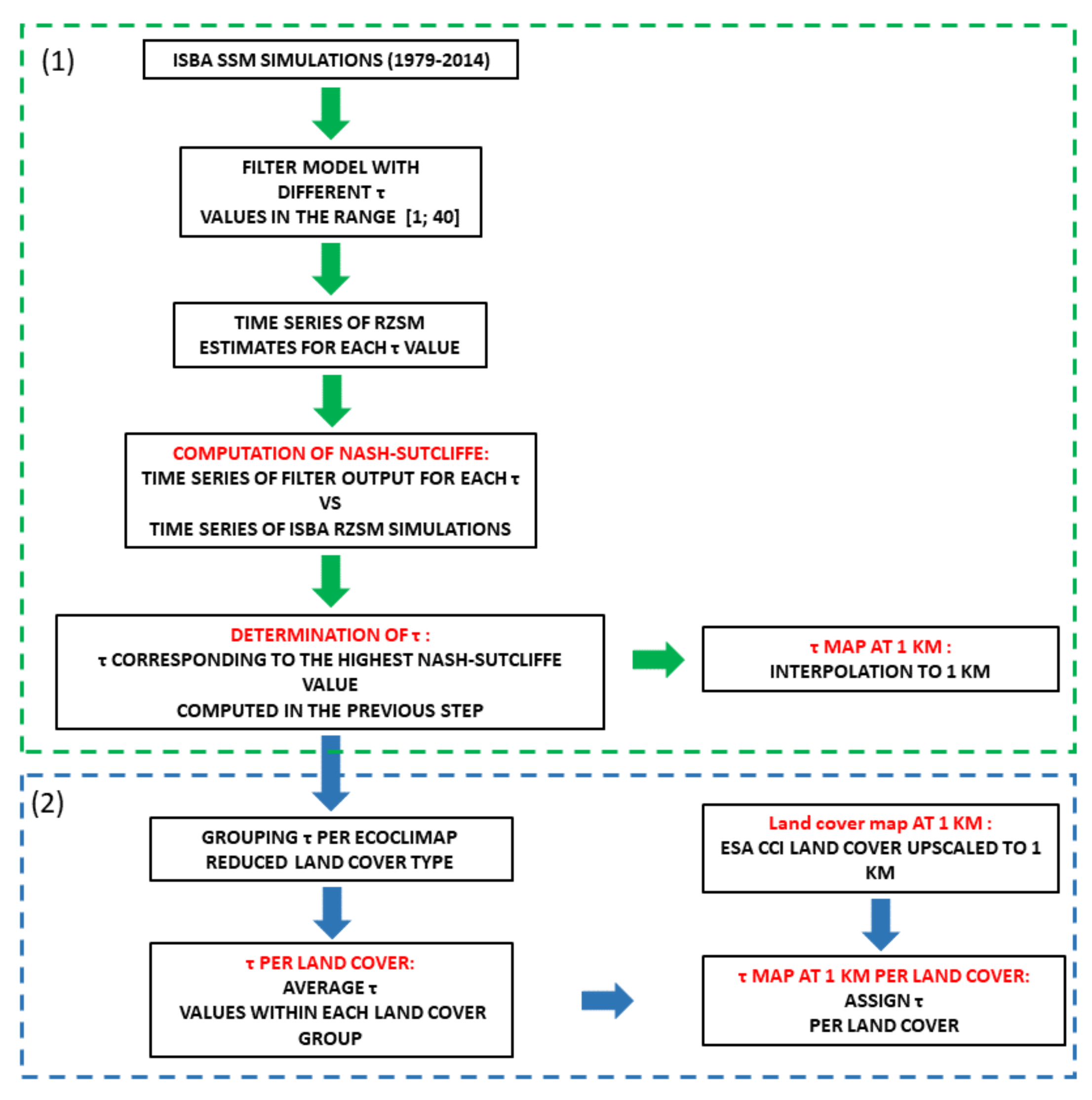
One of the main goals of this study is to obtain a map of the τ parameter, calibrated per land cover type (hereby referred to as τ L C ), values which can then be used regardless of the validation site, provided the land cover type is known. To do so, τ values are first obtained by calibrating it with ISBA-DIF data, hereby referred to as τ I S B A . The steps are detailed below, while a schematic can be found in Figure 2.
As a first step, the ISBA surface soil moisture simulations spanning 1979–2014 are used as an input to the filter model, with different τ parameter values in the range [1; 40]. Since the output of the filter is a measure of the water index rather than the volumetric water content, the ISBA simulations were scaled between [0; 1] prior to using them as input. Root-zone soil moisture estimates are hence obtained for all τ parameter values considered. These estimates are then compared with the ISBA RZSM simulations, and the τ value corresponding to the highest Nash–Sutcliffe (NS) efficiency coefficient obtained is then chosen. The Nash–Sutcliffe efficiency was chosen to evaluate the prediction accuracy. It is defined as one minus the ratio of the error variance of the estimated time series, divided by the variance of the observed time series. NS is equal to 1 in the case of a perfect match between estimations and observations. A value of 0 implies that the estimation error variance is equal to the variance of the observations, while a negative value implies that the estimation error variance is significantly larger than the observation variance. Therefore, values of NS closer to 1 suggest a model with more predictive skill. As the ISBA resolution is 5 km, a table of calibrated τ values was obtained at this resolution. For validation purposes at 1 km resolution, these values were later interpolated to 1 km using a linear interpolation.
The final step consists of obtaining the τ L C values. In order to do so, the  τ I S B A values (at the ISBA native resolution) are used. The values are then grouped depending on the land cover types found within the area, and a mean τ value is then obtained per land cover type, by performing a simple average of the values within the respective class. The land cover types within the study area have been simplified from the ECOCLIMAP dataset (at the ISBA 5 km resolution) into the following six categories: bare areas, urban areas, forests, grass and shrubs, rainfed crops and irrigated crops. A table of τ L C values is hence obtained at the ISBA resolution (5 km).
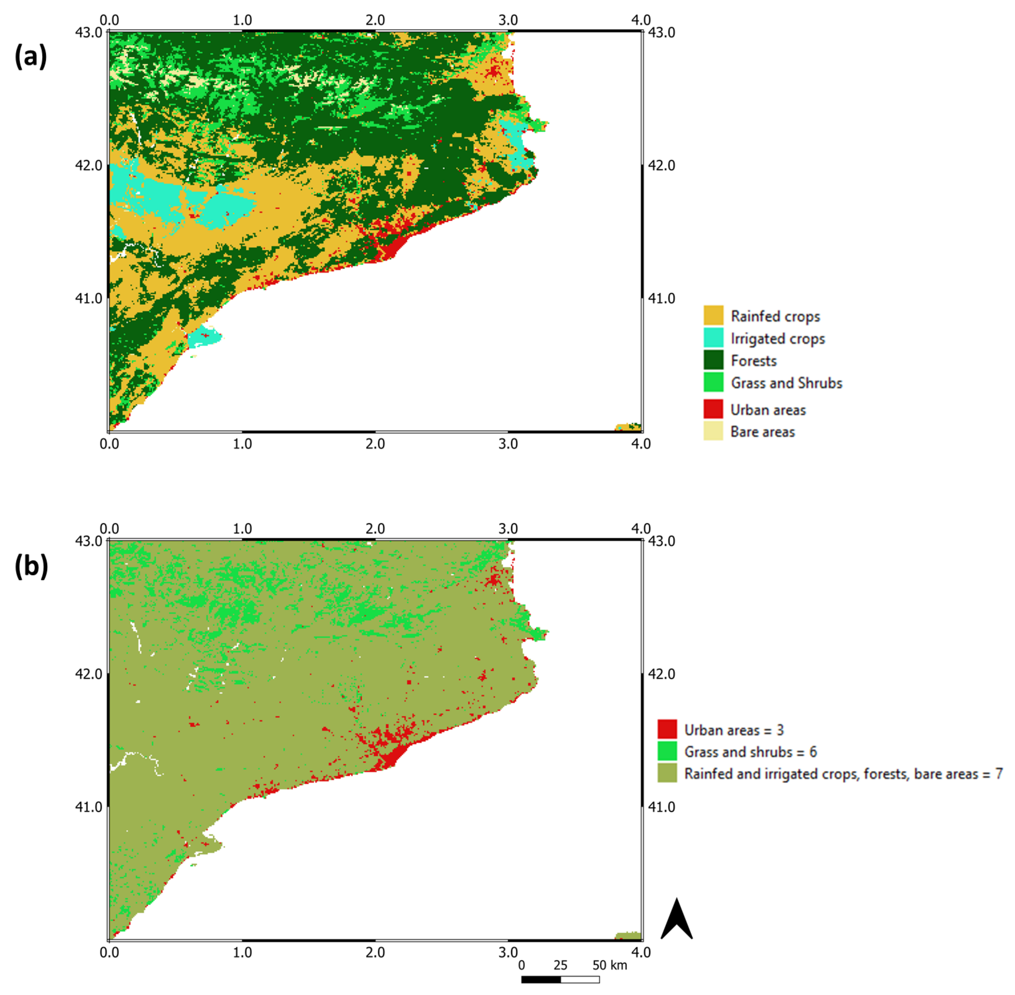
To apply the exponential filter to 1 km-derived SMAP data, a  τ map at 1 km has been created by assigning the corresponding τ value when cross-referenced with a 1 km-derived ESA CCI Land Cover map. Since the original CCI land cover (v2.1.1 2018) is available at a 300 m resolution, the original data has been upscaled to 1 km by using the “mode” method. This method selects the value which appears most often within the selected pixels for the interpolation, which in our opinion, reduces the introduction of further uncertainty at 1 km compared to results obtained if another interpolation method were used.
Figure 3 presents a 1 km resolution map of the reduced ESA CCI land cover, alongside the 1 km resolution map of the τ L C values obtained, within the extended study area.
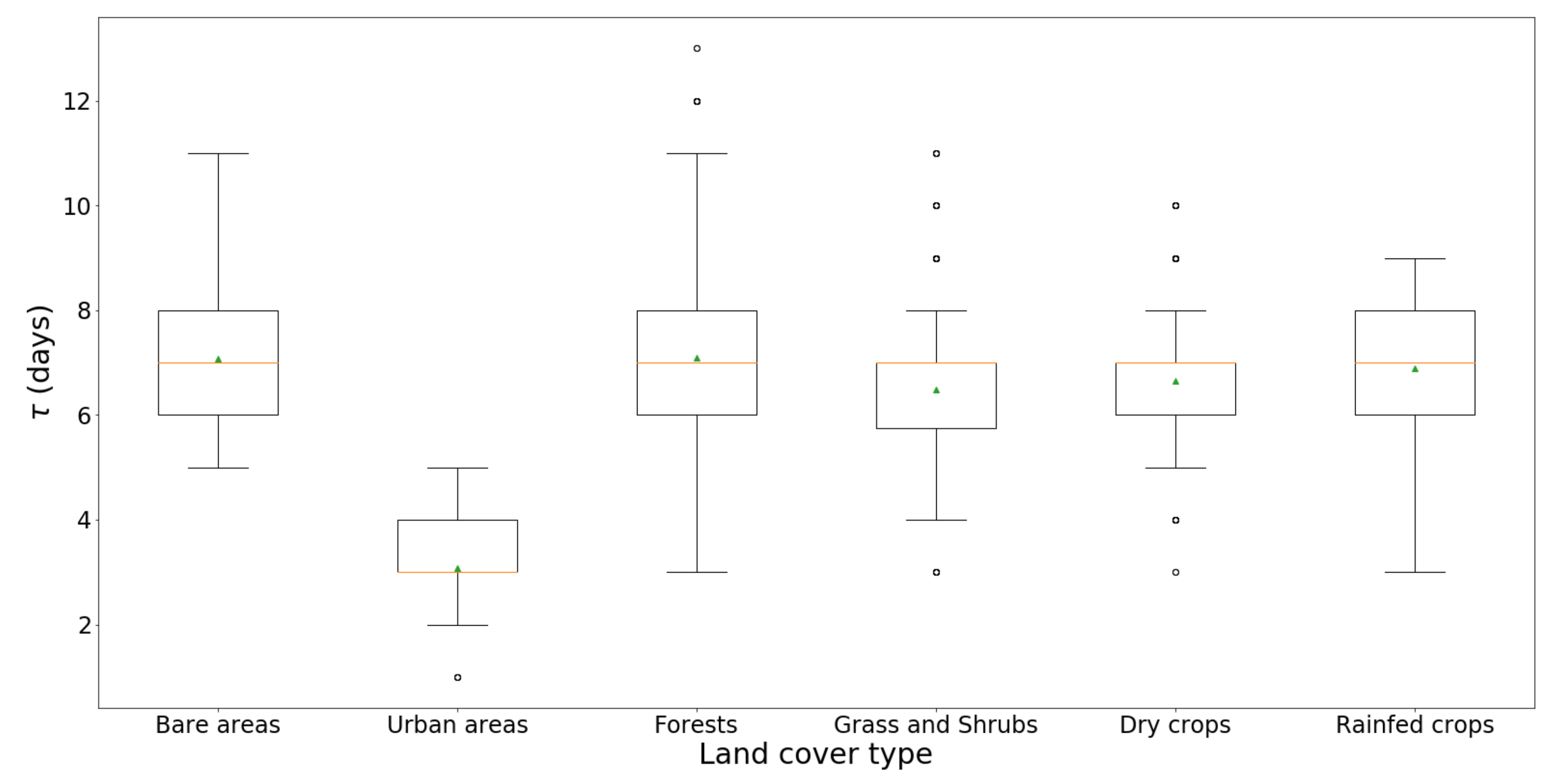
The following τ values (and corresponding standard deviation) were obtained according to the six land cover types considered: 3.08 (1.13) for urban areas, 6.48 (1.36) for grass and shrubs, 6.64 (1.26) for rainfed crops, 6.89 (1.14) for irrigated crops, 7.08 (1.44) for bare areas and 7.09 (1.77) for forests. Figure 4 presents boxplots of the τ L C values. For the application of the filter over the study area, only rounded values (i.e., in terms of days) of the τ parameter have been considered, i.e.: 3 (urban areas), 6 (grass and shrubs), 7 (rainfed crops, irrigated crops, bare areas and forests).

4. Results

In this section, the calibration strategy is first validated, by comparing 1 km SMAP-derived RZSM against in situ measurements over the Terres de l’Ebre and the Algerri Balaguer sites. We focus our attention on the τ L C calibration, as it is one of the goals of this study. Nevertheless, for comparison purposes and to assess the adequacy of this calibration, results obtained from the τ I S B A calibration are also presented (in terms of statistics only). Second, an investigation is carried out on the adequacy of the exponential filter to derive RZSM estimates at different depths, by tuning the τ parameter.

4.1. Validation of τ Calibration

Following the calibration strategy described in Section 3.2, the  τ L C values were used when applying the exponential filter to 1 km SMAP-derived SSM to obtain 1 km RZSM estimates over the entire Spanish study area. The recursive form of the exponential filter in Equation (3) was applied to scaled 1 km SSM between [0; 1]. Since the RZSM estimated by the exponential filter is a measure of the water index more than the volumetric water content, the in situ data have also been scaled prior to comparison, in order to ensure that the error assessment is based solely on the co-variance of the datasets [33].
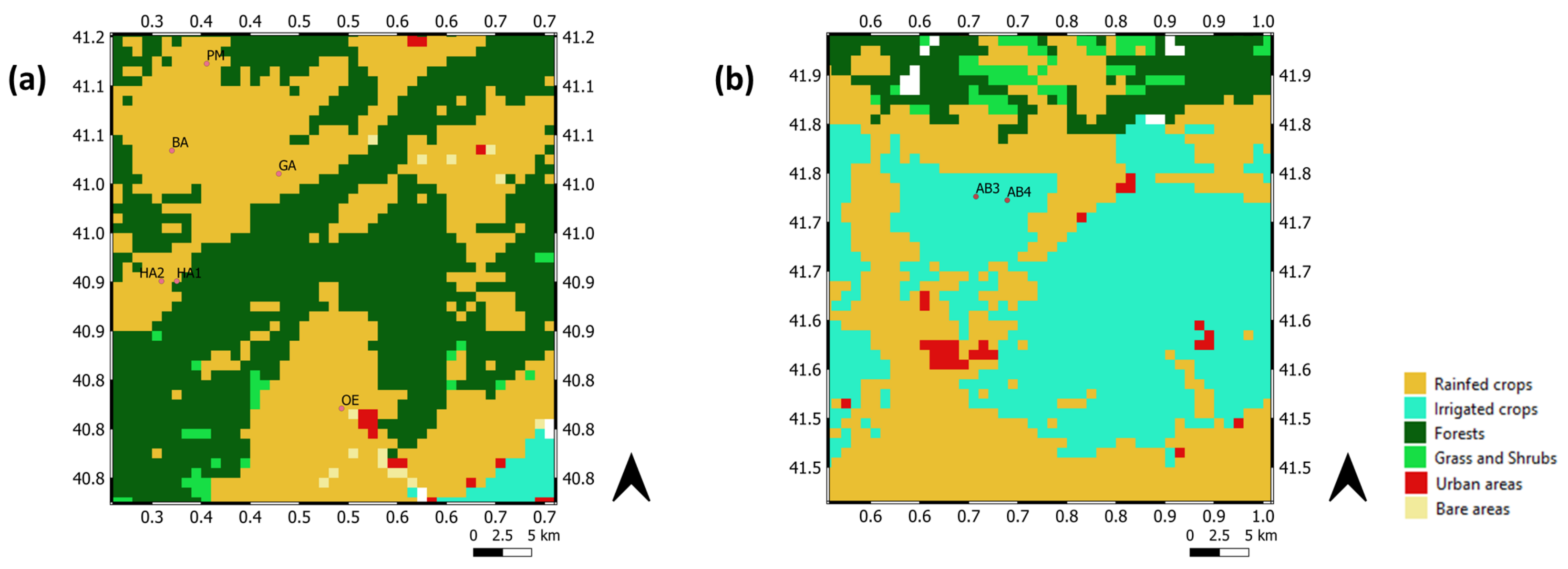
Figure 5 represents the reduced 1 km ESA CCI land cover over the validation areas, along with the validation sites. The sites located in Terres de l’Ebre are all identified as rainfed crops, with monitoring stations located at each of the following sites: Batea (BA), Gandesa (GA), Pobla de Massaluca (PM) and Horta de Sant Joan (HA1 and HA2). In the case of the Observatori de l’Ebre, the values recorded by the sole existing station are hereby referred to as OE. Even though, as mentioned in Section 2.1, the location of the sensor in OE is within a small pine forest, the dominant land cover type at the 1 km scale is rainfed crops. In fact, the small pine forest grew on top of old carob trees, and the surrounding land covers that are dominant within the area are shrubs and almond and olive trees. In Algerri Balaguer, the two sites AB3 and AB4 are identified as irrigated crops.
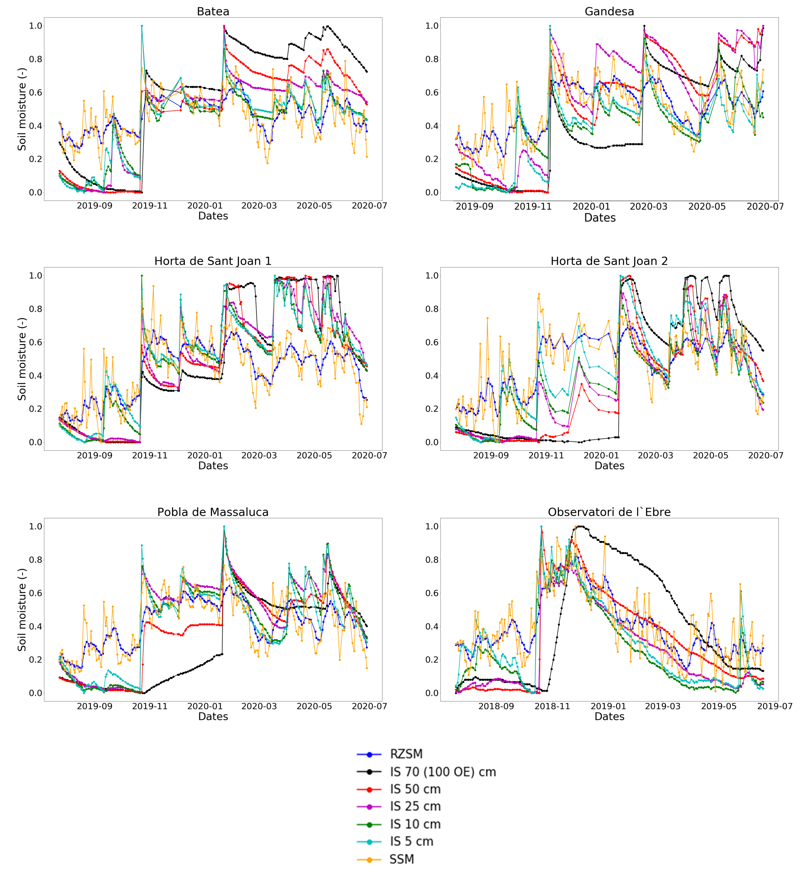
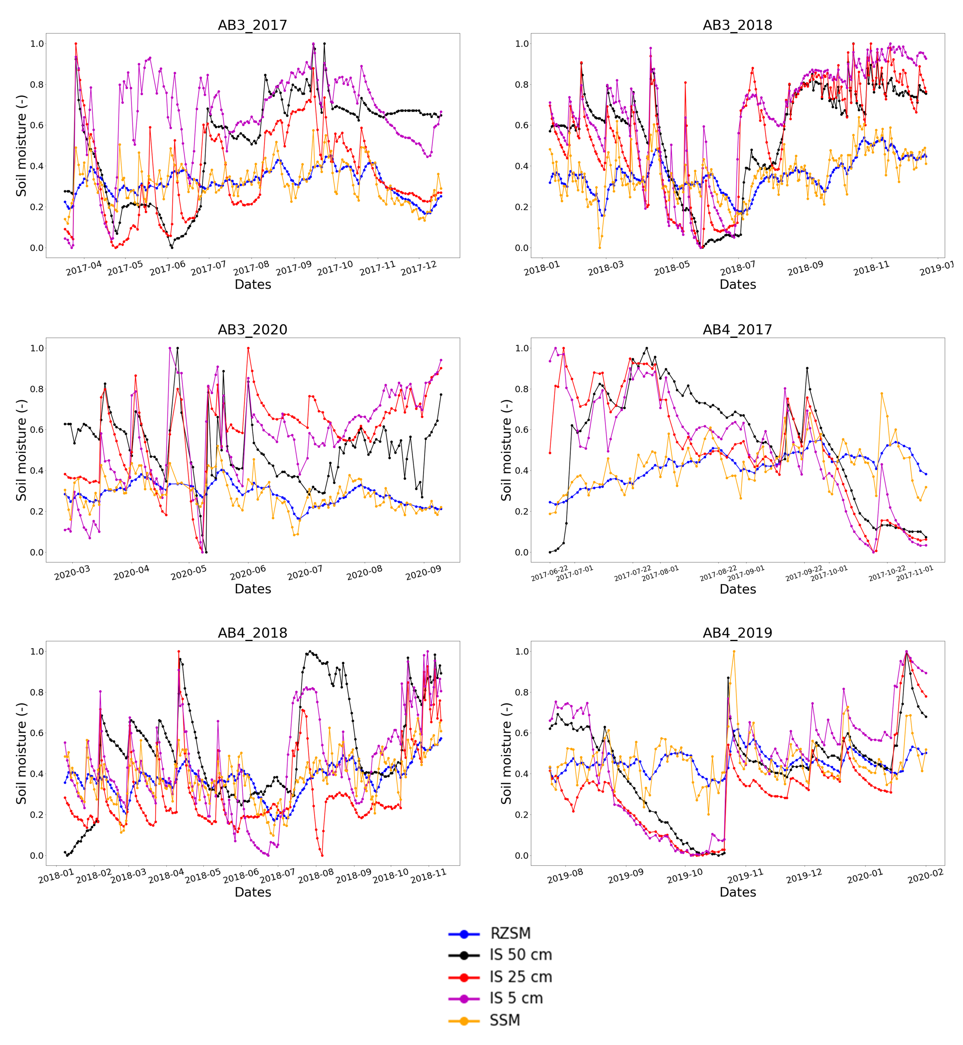
Figure 6 presents the comparison between the time series of the scaled in situ measurements with the SMAP-derived RZSM time series for the sites located in Terres de l’Ebre. In the same manner, Figure 7 presents the same comparison, for AB3 and AB4, for each of the three validation periods considered per site. For visualization purposes, the SMAP-derived SSM is also shown.
In each case, the predicted RZSM was compared with the scaled in situ SM registered by the various sensors located at all the depths: 5, 10, 25, 50 and 70 cm/100 cm (Terres de l’Ebre), and 5, 25 and 50 cm (Algerri Balaguer). For each site, only common days with registered data at all depths have been taken into account, in order to properly compare the datasets at the specified depths.
In both cases, one can see that the estimated RZSM presents a smoothened dynamics as opposed to the remote sensing SSM from which it was derived. Over Terres de l’Ebre, in general, the predicted RZSM can capture general episodes of wetting and drying, albeit with some delays in certain cases. For example, in the case of OE, there seems to be a delay in the response of the RZSM estimates and the observations at 100 cm, in November 2018. Nevertheless, this overlaps quite well with the measurements at other depths. For BA, in November 2019, there is a delay in the response of the predicted RZSM and the scaled in situ SM at 5 and 50 cm, but it overlaps with scaled measurements at the other depths. In the same manner, the same can be said for HA1, where there is a clear delay in the predicted RZSM and scaled measurements at all depths except 70 cm, in December 2019. An example of this delay with respect to all depths, albeit less for 70 cm, is also present for HA2 in February 2020. For PM, in November 2019, for example, the predicted RZSM presents a delay with respect to scaled in situ measurements at 5, 10 and 25 cm, but it overlaps well with the 50 cm depth. All this can be an indication that the predicted RZSM is able, in some cases, to capture some of the delay characteristic to the flow of water content to deeper layers. In the case of Algerri Balaguer, even if the predicted RZSM can capture some episodes of wetting and drying, there is still a rather large difference between the predictions and the measurements. Nevertheless, it seems that the estimated RZSM adjusts more to the in situ observations during rain events. By looking at the time series, one can see that there is a relative difference between the RZSM estimates and the scaled in situ measurements in terms of amplitude: the satellite-derived RZSM have a smaller range of values than the in situ observations. One must keep in mind that the in situ observations have been normalized to be compared to the outputs of the exponential filter (hence ranging between 0 and 1). On the other hand, the exponential filter uses satellite SSM which has been scaled to derive RZSM estimates. This does not imply that the estimated RZSM must have a range between 0 and 1. Moreover, the predicted RZSM series present a higher variability than the in situ observations. A possible explanation for the high variability comes from the high variability of the satellite-derived 1 km SSM used to estimate the RZSM, which themselves present a higher variability than the in situ data.
Statistical results in terms of correlation coefficient, root mean square error (RMSE), bias, slope of the linear regression and the NS efficiency score between predicted RZSM (derived with τ L C and τ I S B A ) and scaled in situ measurements are offered in Table 1 for Terres de l’Ebre, and in Table 2 for Algerri Balaguer.
First, when looking into the statistics obtained when using τ L C as opposed to τ I S B A , one can see that they are very similar (or the same), which validates our approach of calibrating per land cover. The  τ L C values are 7 for all the sites (corresponding to values of both irrigated and rainfed crops). In contrast, the  τ I S B A values are: 6 (OE, AB4), 7 (BA, GA, HA1, HA2 and AB4), 8 (PM). This entails that the only differences are recorded for AB4, OE and PM. The RMSE and bias remain virtually unchanged, while the correlation, slope and NS score differ in some cases by a difference up to 0.02, which from a statistical point of view, is not very representative. In all three cases, the difference in the τ values is only one day, which for AB4 and PM entails slightly better results with τ I S B A , while for OE, it impacts the NS scores at shallower depth (better by 0.01 in the case of τ I S B A ), correlation and NS at 50 cm and 100 cm (better by up to 0.02 and 0.03 respectively with τ L C ). This indicates that the τ L C seems to be a better fit for OE at deeper layers.
One must keep in mind two aspects when trying to interpret the results obtained with the τ L C calibration as opposed to the τ I S B A calibration: (i) even if the sensor is located in a specific cover type, if this cover type is representative at the 1 km scale and (ii) the uncertainty introduced at 1 km when upscaling the reduced original 300 m resolution product. A validation should be carried out in the other land cover types (grass and shrubs, bare areas and forests) to fully assess the potential of the calibration. Unfortunately, we do not have sensors installed in locations representative of these land covers. Nevertheless, referring strictly to the calibration strategy and considering the very subtle difference in statistics, one can conclude that the calibration per land cover type is a viable and adequate method of calibration.
Focusing solely on the results obtained when using τ L C , for Terres de l’Ebre, high values of the NS scores have been registered over the areas, at 10, 25 and 50 cm: 0.51 (25 cm GA) and 0.54 (10 cm HA1) and 0.57 (50 cm OE). In the case of BA, HA2 and PM, however, the highest NS score was registered at 5 cm: 0.44, 0.63 and 0.62, respectively. For BA and PM, there is little difference with the second highest score obtained, at 10 cm: 0.41 (a difference of 0.03) and 0.58 (a difference of 0.04), respectively. However, for HA2, the second highest NS score obtained (at 10 cm), is of 0.49, with a rather significant difference of 0.14. In general, it seems that the lowest NS scores are obtained at the deepest layer, 70 or 100 cm, respectively. This can be an indication of a decoupling occurring at deeper levels. An important thing to note however, is that for all the sites except GA, the RZSM estimates presents the highest correlation with observations at shallower depths of 5 and 10 cm (ranging from 0.77 to 0.88 and from 0.76 to 0.91, respectively), indicating a strong relationship between the surface and the layer immediately below. In general, the RMSE is below 0.20 at 5 and 10 cm for all the sites, and it increases with depth. In terms of bias, BA, GA, HA1 and OE registered the lowest values at deeper layers: 0.001 (BA, 25 cm), 0.001 (GA, 50 cm), 0.025 (HA1, 50 cm), −0.003 (OE, 100 cm). HA2 registers the lowest bias at 5 cm, −0.006, while PM at 10 cm, 0.002. The slope of the linear regression can provide complimentary information on the efficiency of the predictions, as compared to observations [81]. The slope presents higher values at shallower depths of 5 and 10 cm (except OE). Values of 0.35 and 0.54 have been registered at 10 cm (BA, HA2, respectively), 0.53, 0.47 and 0.46 at 10 cm (GA, HA1 and PM, respectively). This is again an indication of the strong relationship between the surface and layers immediately adjacent. For OE, the highest value of the slope has been registered at 25 cm: 0.66.
In the case of Algerri Balaguer, results are contrasting depending on the time period considered. For example, in the case of AB3, the period which yields the best NS scores is 2017, with the highest NS score (0.16) registered at 25 cm. Overall, for 2017, the best statistics are registered at this depth, with a correlation of 0.48, RMSE of 0.20, low bias (0.040), and a slope equal to 0.14. The NS scores registered at all depths for AB3_2018 and AB3_2020 are negative, with the best results obtained at 50 cm in 2018 (NS = −0.39) and at 5 cm in 2020 (NS = −1.31). However, in contrast, the highest correlations at all depths were obtained for 2018, ranging between [0.47; 0.54], as opposed to [0.21; 0.48] for 2017, and [−0.16; 0.33] for 2020. The range of the RMSE is rather high regardless of the depth, ranging between 0.20–0.38 (AB3_2017), 0.30–0.37 (AB3_2018) and 0.26–0.37 (AB3_2020). The bias is rather high as well, regardless of the period, ranging overall between 0.196 and 0.327 (except for 0.040, the lowest value, obtained for AB3_2017 at 25 cm). Very low values of the slope have also been obtained, with the best results obtained at 25 cm (AB3_2017, slope = 0.14) and 50 cm (AB3_2018, slope = 0.18, AB3_2020, slope = 0.11). As a general conclusion, it seems that the 25 cm yields the best results for AB3_2017, 50 cm for AB3_2018, and while the best NS score for AB3_2020 is obtained at 5 cm, the rest of the statistics are better at 50 cm as well.
In the case of AB4, some of the same contrasting results can be observed. However, in contrast, it seems 2017 is the worst period for this location, with negative values obtained for NS (the highest being −0.26 at 50 cm), for the correlation (the highest being −0.02 at 50 cm) and the slope (the highest being −0.00 at 50 cm). For AB4_2018 however, results improve in terms of correlation and NS (although the NS scores remain low). A strong dependence is observed between the predicted RZSM and the surface layer, with the highest correlation, slope and NS scores obtained at 5 cm: 0.48, 0.17 and 0.13, respectively. In the case of AB4_2019, it seems that the lower depths provide a better correspondence in terms of correlation (0.28 at 25 cm), slope (0.07 at 25 cm), and NS score (0.06 at 50 cm). The RMSE for AB4, remains, in general, high, ranging overall between 0.19 and 0.34, while the bias is ranges overall between −0.137 and 0.148.
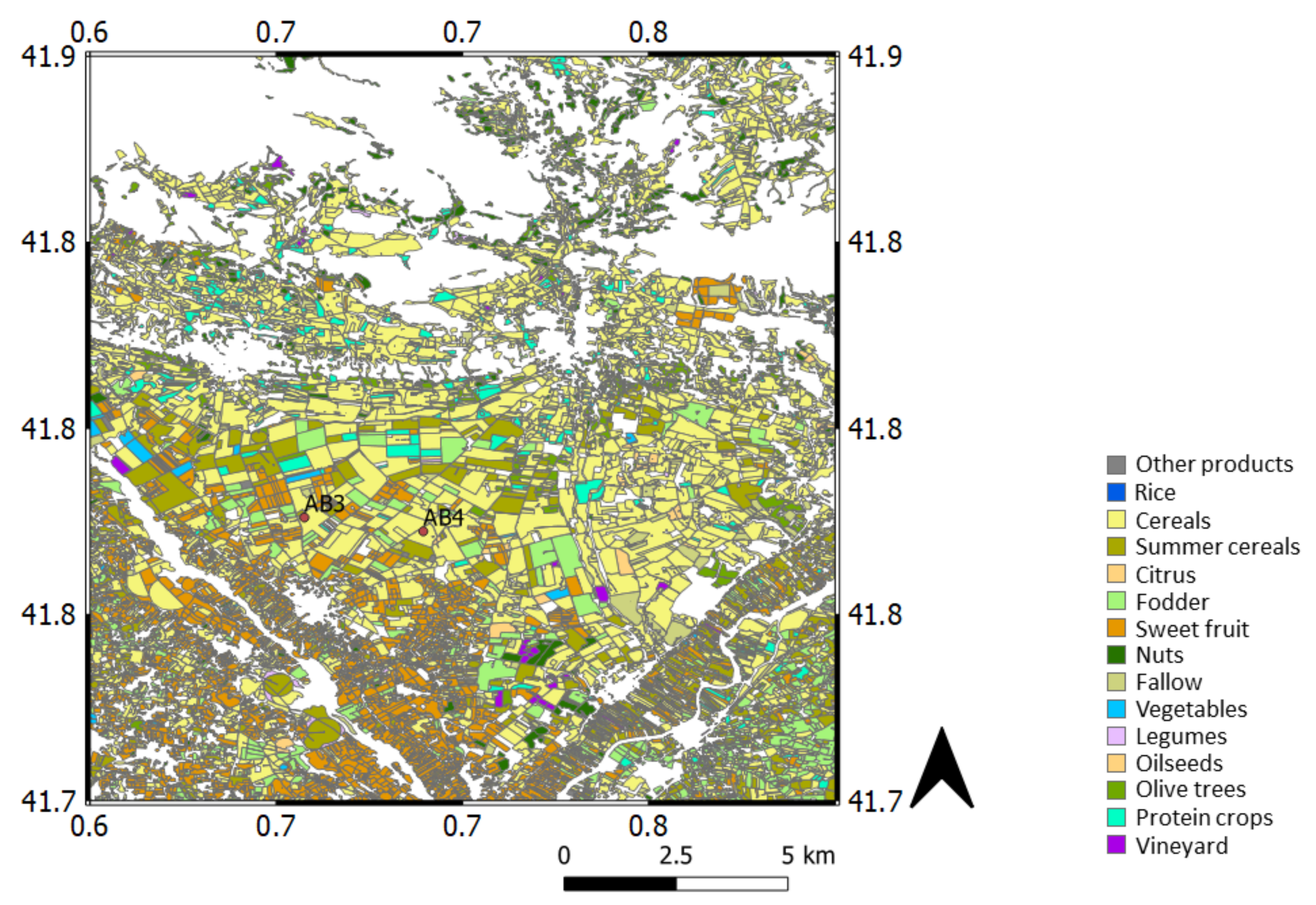
The results are poorer for Algerri Balaguer, especially when looking at the NS scores overall, and the correlation in some cases. In order to try and find a possible explanation to these varying and contrasting results, we have taken a look at the main crops present within the Algerri Balaguer area, as seen in Figure 8. The map was downloaded from the Catalan Geographical Information System of Agricultural Parcels (Sistema de Información Geográfica de Parcelas Agrícolas, SIGPAC (http://sig.gencat.cat/visors/Cultius_DUN_SIGPAC.html), accessed on 3 January 2021) and presents, at parcel scale, the main crops found within the entire Catalonia. As can be seen, there is a very high heterogeneity present within the area. This can be a possible explanation for the poor results obtained for Algerri Balaguer, coupled with different irrigation practices present within the 1 km pixel. Therefore, the RZSM present in the area is actually rather “non-homogeneous”, so when compared to an estimated RZSM assumed homogeneous at the 1 km scale, discrepancies appear, as reflected in our results. This effect is not visible when precipitation takes place though, where, as seen from the time series, the estimated RZSM adjusts more to the in situ observations. This implies conditions over the area become homogeneous at the 1 km scale, and, as seen from Terres de l’Ebre, it translates into a better correspondence being obtained.

4.2. τ —Depth Sensitivity Study

A study regarding the filter’s sensitivity to the τ parameter has been carried out, by varying the parameter to take values between [10; 90], with a time-step of 10 days. The main motivation behind this study was generated by a mismatch between the depth of the SSM used to initially calibrate τ (before averaging the values per land cover type) and the sensing depth of the SMAP sensor. More specifically, the remote-sensing-derived SSM might have a shallower depth than the SSM estimated by the ISBA-DIF land surface model. This would implicate than when deriving the RZSM estimates from remote sensing, these could be representative of “shallower” depths. This seems to be corroborated by almost all the sites (especially the ones in Terres de l’Ebre) providing the best correlation and NS score at 10 and 5 cm. Therefore, the main insight this sensitivity study aims to provide is whether the RZSM estimates would correlate better with in situ observations at deeper level, as well as if the NS score increases with τ for deeper layers. Each τ value in the interval was used as input to the exponential filter, and RZSM estimates were obtained by using the SMAP-derived 1 km SSM.
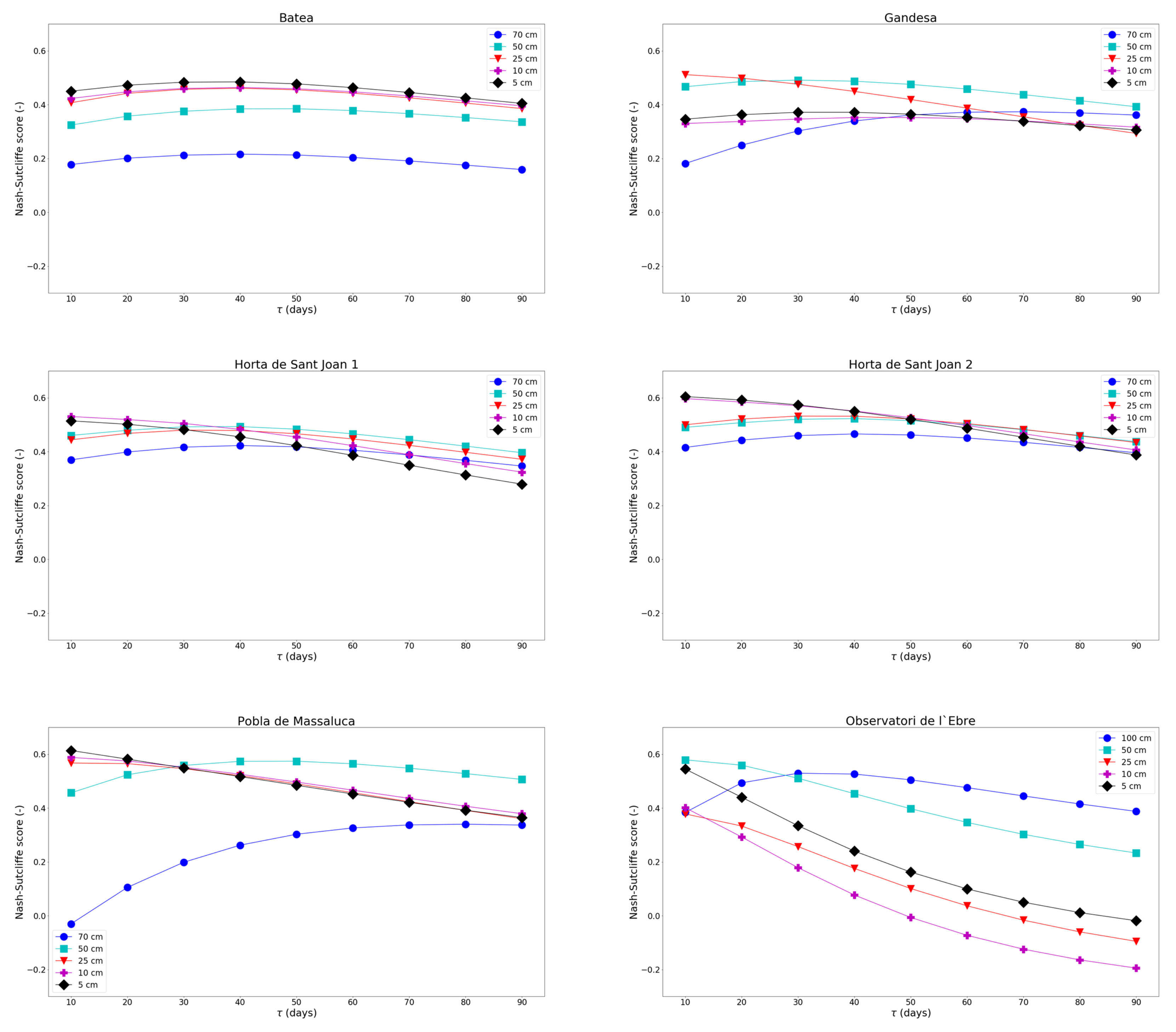
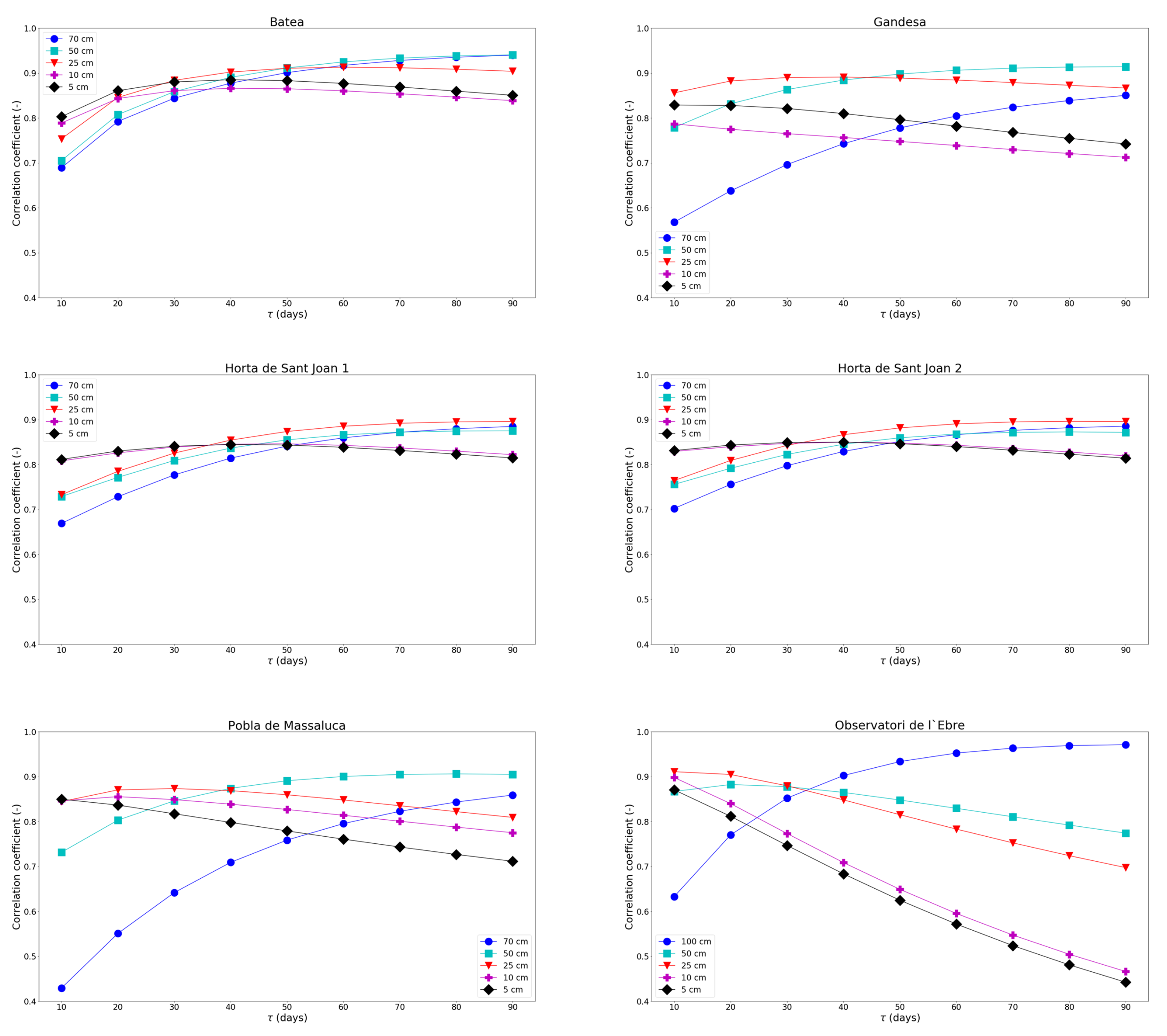
Figure 9 and Figure 10 present the evolution of the NS score and correlation at different depths, with respect to the evolution of τ , for the sites located in Terres de l’Ebre.
When looking at the influence of τ on the two statistics for Terres de l’Ebre, several general comments can be made. The NS score increases with τ at deeper levels (70/100 cm and 50 cm) for all the validation sites, up to a value, and then it starts decreasing, while the correlation at the same levels also increases with τ up to a certain value, but then it tends to stabilize. It seems (at the root-zone layers) that there is an optimal value for τ at which the NS reaches a highest score, after which there is a decoupling, with the same not being true for the correlation, as it constantly increases.
More specifically, in the case of BA, the NS score at all depths constantly increases until τ = 40(50), and then it slowly decreases. The best NS registered at BA is always found at 5 cm, regardless of the variation of τ , followed by 10 and 25 cm respectively, which show very little difference.
In the case of GA, the best NS is registered at 25 cm for τ between 10 and 20, after which the best NS scores are found for the 50 cm depth. For the 5, 10 and 50 cm depths, it seems the optimal τ is around 40, while for the 70 cm depth, an optimal value of 70 is found.
HA1 and HA2 present strong dependence with the shallower depths, which, even though they possess a NS value which decreases with τ , still provide the best NS scores overall. For HA1, there is a shift from 10 cm (best NS score until τ = 30) to 50 cm (best NS scores from τ = 40). A similar shift is observed for HA2, with the 5 cm providing the best NS scores until τ = 40, after which the 25 cm depth yields the best results (from τ = 60).
The same trend is observed at PM, where the shift occurs from τ > 20, switching from 5 cm to 50 cm. BA, HA2 and PM have been previously identified as sites where there is a strong dependence observed with the surface layers, dependence which seems to be valid up to large values of τ .
OE (alongside GA) is a good example where a strong dependence is found from the start at lower layers (50 and 25 cm, respectively). The NS score at all depths except 100 cm decrease with τ , while for 100 cm, the optimal τ is 40. The best NS values for OE are found at 50 cm for τ < 30, after which a switch is made to 100 cm.
In conclusion, in order to obtain a strong dependence with the root-zone layers (except BA), the optimal τ values for each site are: 30 (GA, 50 cm), 40 (HA1, 50 cm), 60 (HA2, 25 cm) and 40 (PM, 50 cm).
Correlation-wise, for all the sites in Terres de l’Ebre at shallower depths (5, 10 cm), it either increases up until a value of τ and then decreases, or decreases from the start. Hence, correlation for GA, OE and PM decrease with τ at these depths, while for BA, HA1 and HA2, it increases up to τ = 30, after which it decreases. At 25 cm, for OE, correlation decreases with τ , while at PM and GA it increases only up to 30. At 50 and 70 cm, for all sites except OE (where this effect is observed only at 100 cm), correlation steadily increase, regardless of the τ value. Therefore, even if it seems, correlation-wise, the higher the τ , the better with respect to the correspondence at lower layers, there is a trade-off with the NS score which must be taken into consideration (NS decreasing after a certain threshold).
The same analysis (not shown) was done over the sites in Algerri Balaguer; however, regardless of the τ variation, the high heterogeneity present in the study area cannot be accounted for, and poor results were still predominant. This is to be expected, since the 1 km SSM used to derive the RZSM is not able to capture said heterogeneity. The NS score was predominantly negative, the only exception being AB3_2017 (for the 25 cm depth), where it varied very little with τ , and with low values around 0.03–0.14. In terms of correlation, the analysis showed that in general, it decreased with τ , with a notable exception being AB3_2017 (for the 50 cm depth), where it increased with τ , from 0.23 to 0.63. Nevertheless, it seems difficult to draw a common conclusion with respect to the influence of the τ parameter on the evolution of the correlation and NS score for Algerri Balaguer, which can partly, as explained before, be due to the very high heterogeneity present within the area, and also to the in situ observations not being representative of the 1 km scale of the estimated RZSM.
This sensitivity study has shown that the filter is rather sensitive to changes in the τ parameter, and that in general, the NS score and correlation increase at lower depths with the increase of τ over homogeneous sites, such as Terres de l’Ebre. Three sites in particular show a very strong relationship with the 5 and 10 cm layers, until  τ switches to high values (>30). Even though these sites have been classified as rainfed crops, the same as two other sites where this dependence is not seen, there seems to be an indication that there might be other factors that influence rather strongly the filter model. Moreover, there seems to be an optimal τ value at which the estimated RZSM shows strong NS scores with the root-zone layers, after which there seems to be a decoupling. Therefore, even though the τ derived from ISBA (and then averaged per land cover type) seems to correspond largely to the surface layer, there is evidence (over the rainfed fields at least) that a larger τ (30–40) is needed to obtain better correspondence in the root zone.

5. General Discussion

This study provides several insights into the exponential filter methodology [54] of deriving RZSM from downscaled SMAP SSM data. The main goal is to assess the validity of a calibration per land cover type, which would be a powerful asset in calibrating the filter independently of the SSM given at the filter input (whether it might be in situ, model or satellite-derived). The calibration has yielded values of 3 (corresponding to urban areas), 6 (corresponding to grass and shrubs) and 7 (corresponding to rainfed crops, irrigated crops, forests and bare areas). The methodology was validated in rainfed (Terres de l’Ebre) and irrigated crops (Algerri Balaguer). This latter value is consistent to the average τ values found in other studies: 6 [51], 8 and 9 [33].
Previous studies [33,51,61,82] reported good correspondence between the predicted RZSM and the root-zone observations at 30 cm, which is mostly corroborated by our study as well (when comparing at 25 cm). The correlation coefficient (at 25 cm) retrieved over the sites in Terres de l’Ebre ranges between 0.71 and 0.90. For Algerri Balaguer, the correlation coefficient at 25 cm ranges between 0.28 and 0.48 (excluding two negative values of −0.56 and −0.16). For example, [51] found a correlation coefficient between estimated RZSM (from in situ data corresponding to SMOSMANIA and SMOSREX datasets) and observations at a 30 cm depth between 0.49 and 0.97 over the South of France. The high correlations obtained by [51] could be explained by the fact that they used the in situ SSM to derive the RZSM over their study sites. In our case, we used the SMAP SSM, downscaled at 1 km through DISPATCH [67], in order to derive 1 km resolution RZSM estimates, which were subsequently compared to the in situ observations in the root zone. This results in a bigger difference between the estimations and the observations, due to the already inherent difference between the remote sensing SSM and in situ SSM observations. Moreover, our retrieved RZSM presents higher variability than the in situ observations, which is explained by the high variability present in the remote sensing SSM products. A possible explanation for the poor results obtained in Algerri Balaguer is the very high heterogeneity found within the area (within the 1 km pixels), as opposed to the more homogeneous sites located in Terres de l’Ebre. This effect seems to be toned down during large-scale homogeneous events such as rainfall, where a better adjustment is obtained between estimations and observations. This could prove an interesting point, and would serve to evaluate the effective precipitation.
On the other hand, [33] have found correlation coefficients between 0.57 and 0.24 when comparing their estimates with the observations of two stations located in the United States. In the case of [33], they have used SMOS SSM at its native resolution (40 km) to derive RZSM estimates. The coarse resolution of the native SSM product can explain the poorer results in terms of correlation, since there is a large-scale mismatch between the SMOS observations and the in situ data. In our study, we have showed that using downscaled 1 km resolution SMAP SSM is more representative of the study area, and subsequently yields better correlations than by using the native SMAP resolution. Since the current remote sensing products have a resolution that proves too coarse for agricultural and hydrological applications, using a downscaling methodology before deriving RZSM from satellite SSM can significantly improve the results.
However, an important aspect to point out in our study is the strong correlation found with the surface layers (5 and 10 cm, for BA, HA1, HA2 and PM, with  τ calibrated per land cover). The correlation at 5 cm ranged between 0.77 and 0.84, while the correlation at 10 cm between 0.76 and 0.83. This is an indication of the very strong coupling between the surface represented by the satellite-derived product and the layers immediately adjacent to it. The same observation is made by [62], who have done a performance evaluation of the exponential filter and of an entropy-based model at different depths (10, 20, 50 and 100 cm), and have found that the highest correlation for the exponential filter is at 10 cm. As the depth increases, the correlation decreases, indicating the limitations of the model to estimate RZSM solely from surface observations. This is consistent with literature [63,83], which stated that the surface and root zone get decoupled and exhibit very weak relationships.
In terms of the NS score, we have obtained adequate and good values at 25 cm for Terres de l’Ebre, ranging between 0.39 and 0.56. Ref. [33] have reported values (at 20 cm) ranging between 0.45 and 0.91 and between −1.82 and 0.60, for their two study areas, while [51] have reported values (at 30 cm) between 0.56 and 0.93, and between 0.37 and 0.88 (with some negative values also recorded), for their respective study areas. Ref. [62] have registered poorer results in terms of the NS score at a 20 cm depth, ranging between −0.42 and 0.73 over their respective study sites. Nevertheless, they have found better NS scores at shallower depths (10 cm), ranging between 0.04 and 0.91. This supports our findings as well, with a higher registered NS score at 10 cm depth (as compared to 25 cm) for four sites in Terres de l’Ebre, ranging between 0.41 and 0.58. Moreover, we have found an even stronger coupling with the surface (5 cm) for these sites, with NS ranging between 0.44 and 0.63. For the Algerri Balaguer sites, poor NS scores have been obtained, ranging between −2.57 and 0.16, with mostly negative values, regardless of the site and time period considered.
In the case of the stations located in Terres de l’Ebre, there is a constant overestimation observed in summertime 2019, which, depending on the site, can last until January/February 2020. Ref. [65] have also reported large overestimations when comparing their RZSM estimates (from ERS-scat) with ISBA data over the SW of France, in summertime, which corroborated part of our findings. Ref. [62] have also noted poor performance of the filter in summertime, which they explained as the filter model being directly related to surface soil evaporation; at lower layers, the relationship should take into consideration the vegetation evapotranspiration as well, a fact which it is not able to capture well. This translates into summertime drying events (little rainfall and a strong evapotranspiration) decoupling the surface and lower layers, with the filter model failing to distribute the moisture properly.
All things considered, the strategy of calibrating per land cover type has proven adequate, as it was able, in general, to capture the dynamics and provide high NS scores and good correlations at 10 and 25 cm, respectively, when validating over rainfed crops. Even though poorer statistics have been observed over the irrigated sites, due to the high heterogeneity present, in general, the highest correlations and NS score have been obtained at 25 and 50 cm, indicating that the filter is able to estimate a RZSM value which corresponds better to deeper layers for irrigated fields as well. When interpreting the results, one must also keep in mind that τ L C was obtained from τ I S B A , by averaging those values per vegetation cover type at the native (5 km) ISBA resolution. On the one hand, calibrating τ with ISBA-DIF data is highly dependent on the accuracy of the LSM estimations, as these τ values were later averaged per land cover type. On the other hand, these averaged values were later assigned to 1 km pixels of a derived ESA CCI land cover product at a 1 km resolution. In order to obtain this land cover map at 1 km, the original 300 m resolution ESA CCI land cover product was upscaled by selecting at the 1 km scale the dominant land cover present at the original scale. This also represents a source of uncertainty, albeit we have chosen an upscaling method which reduced the uncertainties when upscaling to 1 km.
In addition to the main goal of assessing the adequacy of calibrating τ L C , a sensitivity study was performed, by tuning the τ parameter. This was prompted by a possible mismatch in the depth of the SSM estimated by ISBA-DIF and the SSM measured through remote sensing. This is important as the τ parameter was calibrated with ISBA-DIF data prior to averaging values per land cover type. Therefore, the  τ thus obtained might not be the same when using remote sensing SSM data as input to the filter. The remote sensing data is representative of a shallower depth than the LSM data, which would mean that using the τ calibrated (at an intermediary step) with LSM data might yield RZSM estimates corresponding to shallower depths. Hence, the  τ parameter increased with a 10-day time-step between [10; 90] to assess its influence on the RZSM estimates at different depths. Results are consistent over all sites in Terres de l’Ebre, in that as τ increases, so does the correlation and NS score at deeper levels (70/100 cm and 50 cm), while decreasing at the surface level. This is an indication that the filter presents certain sensitivity to τ , and a better coupling can be obtained at deeper levels for higher values of τ . However, for three of the study sites in Terres de l’Ebre, the overall best results in terms of NS score were still obtained for surface depths (5 cm and 10 cm respectively), which would suggest these locations in particular, the coupling is very strong with the surface and the filter is not able to overcome this effect. However, two other sites in Terres de l’Ebre sites, in contrast, constantly obtain the best results at lower depths (25 and 50 cm) with the increase of τ . In particular, for OE, there is a very strong coupling with the 50 and 25 cm layer, even for τ L C . Even though the assigned land cover at 1 km is rainfed crops, the sensor is in a small pine forest. The  τ value obtained for forest and rainfed crops is the same (7); however, the estimated RZSM has a stronger link with the in situ data from forest rather than the in situ data from cropland. Hence, it would seem that a “real” validation (as in more representative of the actual conditions in the field), yields better results at deeper layers in forests rather than in croplands.

6. Conclusions

This paper assesses the adequacy of a pseudodiffusivity parameter τ calibrated per land cover type in the use of the recursive form [66] of an exponential filter [54] to retrieve scaled RZSM estimates from 1 km downscaled SMAP SSM data. The recursive form is chosen due to its capability of lowering computational time.
The “pseudodiffusivity” parameter τ of the filter is calibrated over an area in Catalonia, Spain, by land cover type. First of all, the ISBA-DIF scaled SSM simulations are used as an input to the filter, for  τ values ranging between 1 and 40. The resulted RZSM is then compared to the ISBA-DIF RZSM simulations, and the τ value which yields the best Nash–Sutcliffe score is then kept, resulting in a map over the entire study area at the native ISBA resolution (5 km). The second step of the calibration strategy consists of averaging the τ values obtained previously per different land cover types, using the ECOCLIMAP map at the ISBA resolution, reduced to six main classes: rainfed crops, irrigated crops, forests, grass and shrubs, bare areas, urban areas. Once these values have been computed for each land cover type considered, a map is created at 1 km resolution, by assigning the τ value corresponding to the 1 km ESA CCI-derived land cover. This map is obtained from the original 300 m resolution product, by upscaling it to 1 km.
The SMAP SSM is downscaled to 1 km by using the DISPATCH [67] methodology prior to using it as input to the filter. The estimated RZSM is then compared to scaled in situ observations, at different depths, over two areas: Terres de l’Ebre (five sites–BA, GA, HA1, HA2, PM and OE, corresponding to rainfed crops) and Algerrri Balaguer (two sites–AB3 and AB4, corresponding to irrigated crops). Good results are obtained at 10 and 25 cm (50 cm for OE) in terms of the Nash–Sutcliffe score for Terres de l’Ebre: 0.41 (10 cm BA), 0.51 (25 cm GA), 0.54 (10 cm HA1), 0.49 (10 cm HA2), 0.58 (10 cm, PM) and 0.57 (50 cm, OE). For Algerri Balaguer, the NS scores obtained are poorer, with the best reported values being 0.16 (AB3_2017, 25 cm) and 0.13 (AB4_2018, 5 cm). Strong correlations have been observed in general over all sites at the shallower depths of 5 and 10 cm, indicative of a strong coupling of the surface to the layers adjacent. Moreover, for BA, HA2 and PM the best NS value is obtained at 5 cm: 0.44, 0.63 and 0.62, respectively.
To assess the adequacy of the calibration strategy, RZSM estimates obtained with τ L C have been compared against estimates obtained with τ I S B A . No significant differences in terms of statistics have been registered, leading to the conclusion that the calibration per land cover type is an adequate calibration strategy.
Given the strong dependence found at 10 (and 5) cm, a sensitivity study was carried out, by varying τ values between 10 and 90, with a 10-day time-step. It has been found that in general, with increasing τ , the NS score and correlation increases with the depth, for Terres de l’Ebre. Except three sites in particular, which show very strong correspondence to the 5 and 10 cm layers, the study has shown that the correspondence shifts to a deeper layer once τ reaches a certain high value.
This study underlines the potential of the recursive formulation of the exponential filter to retrieve high-resolution RZSM estimates from downscaled SMAP SSM data. Satellite measurements of SM are valuable presently especially due to their global spatial coverage, which makes the application of the exponential filter easier at any given location, as opposed to using in situ observations. However, their coarse resolution means a large-scale mismatch is present when the application domain is agriculture or hydrological, where SM is needed at high-resolution. By using DISPATCH to downscale SMAP SSM, and using it as an input to the filter, we address this scale mismatch, obtaining RZSM estimates which are more representative of the study domain. Moreover, in order to fully take advantage of the global coverage of satellite data and eliminate the need for site-specific calibration, an independent calibration, per land cover type, proves a useful resource. The adequate results that are obtained provide confidence in the applied approach. Nevertheless, there are some things to be kept in mind when interpreting said results. First, as an intermediate step, τ is calibrated from ISBA-DIF data, meaning τ is calibrated with RZSM simulations which are integrated over the entire profile (and it introduces a model dependency), and at the ISBA resolution. The best results were obtained when comparing the estimated RZSM with the 5 cm, 10 cm and 25 cm scaled in situ observations, with the results then decreasing with depth. This is an indication that the obtained τ is better suited for that depth, with larger values being needed to obtain better correlations and NS scores at lower depths. Another aspect to be taken into consideration is related to the second step of the calibration strategy, which attributes τ values per land cover type at the original ISBA resolution. In order to obtain a map of τ at the 1 km resolution need for our study, we have derived a 1 km land cover map from the original 300m ESA CCI land cover product, by upscaling it, which can introduce some uncertainty with respect to the actual land cover type present.
This study shows the potential of retrieving high-resolution RZSM estimates from remote sensing data, with a calibration depending solely on the land cover type present within the area. As for potential future studies, the application and validation of the methodology over other land cover types and in other climatic zones than the ones presented in this study can be investigated. Moreover, the influence of the soil texture in the calibration of the filter can be a further potential perspective worth considering. Additionally, one can investigate the use of a global τ map with the values obtained in the present study, which would facilitate the application of the exponential filter regardless of the study area. Furthermore, the 1 km resolution can sometimes be too “coarse” if the actual validation sites are in a highly heterogeneous area (as in the case of Algerri Balaguer). Future research can investigate using higher resolution (e.g., several hundreds of meters) remote-sensing-derived SSM, coupled with a corresponding higher resolution land cover map to estimate high-resolution RZSM that can be more representative of these heterogeneous areas.

Author Contributions

Conceptualization, V.-G.S., G.I. and M.-J.E.; methodology, V.-G.S. and G.I.; software, V.-G.S. and G.I.; validation, V.-G.S.; formal analysis, V.-G.S.; investigation, V.-G.S. and G.I.; resources, V.-G.S. and G.I.; data curation, V.-G.S., G.I., P.Q.-S. and J.M.V.; writing—original draft preparation, V.-G.S.; writing—review and editing, V.-G.S., G.I., M.-J.E., P.Q.-S. and J.M.V.; visualization, V.-G.S.; supervision, M.-J.E.; project administration, M.-J.E.; funding acquisition, V.-G.S. All authors have read and agreed to the published version of the manuscript.

Funding

This research was funded by the Torrres Quevedo program of the Spanish Science Ministry, MICINN (grant number PTQ-16-08766).

Institutional Review Board Statement

Not applicable.

Informed Consent Statement

Not applicable.

Data Availability Statement

Not applicable.

Acknowledgments

This study was supported by the HUMID project (CGL2017-85687-R, AEI/FEDER, UE) and the European Commission ERA-NET COFUND WATERWORKS 2015 Program (Water4Ever project).

Conflicts of Interest

The authors declare no conflict of interest.

References

  1. Pal, J.S.; Elthair, E.A.B. Pathways relating soil moisture conditions to future summer rainfall within a model of the land-atmosphere system. J. Clim. 2001, 14, 1227–1242. [Google Scholar] [CrossRef]
  2. Basara, J.B.; Crawford, K.C. Linear relationships between root-zone soil moisture and atmospheric processes in the planetary boundary layer. J. Geophys. Res. 2002, 107, 4274. [Google Scholar] [CrossRef] [Green Version]
  3. Daly, E.; Porporato, A. A Review of Soil Moisture Dynamics: From Rainfall Infiltration to Ecosystem Response. Environ. Eng. Science 2005. [Google Scholar] [CrossRef]
  4. Kerr, Y.H.; Waldteufel, P.; Wigneron, J.P.; Delwart, S.; Cabot, F.; Boutin, J.; Escorihuela, M.J.; Font, J.; Reul, N.; Gruhier, C.; et al. The SMOS Mission: New Tool for Monitoring Key Elements of the Global Water Cycle. Proc. IEEE 2010, 98, 666–687. [Google Scholar] [CrossRef] [Green Version]
  5. Entekhabi, D.; Njoku, E.G.; O’Neill, P.E.; Kellogg, K.H.; Crow, W.T.; Edelstein, W.N.; Entin, J.K.; Goodman, S.D.; Jackson, T.J.; Johnson, J.; et al. The Soil Moisture Active Passive (SMAP) Mission. Proc. IEEE 2010, 98, 704–716. [Google Scholar] [CrossRef]
  6. Kerr, Y.H. Soil moisture from space: Where are we? Hydrogeol. J. 2007, 15, 117–120. [Google Scholar] [CrossRef]
  7. Wagner, W.; Bloschl, G.; Pampaloni, P.; Calvet, J.C.; Bizzari, B.; Wigneron, J.P.; Kerr, Y. Operational readiness of microwave remote sensing of soil moisture for hydrologic applications. Nord. Hydrol. 2007, 38, 1–20. [Google Scholar] [CrossRef]
  8. El Hajj, M.; Baghdadi, N.; Bazzi, H.; Zribi, M. Penetration analysis of SAR signals in the C and L bands for wheat, maize, and grasslands. Remote Sens. 2018, 11, 31. [Google Scholar] [CrossRef] [Green Version]
  9. El Hajj, M.; Baghdadi, N.; Zribi, M. Comparative analysis of the accuracy of surface soil moisture estimation from the C-and L-bands. J. Appl. Earth Obs. Geoinf. 2019, 82, 101888. [Google Scholar] [CrossRef]
  10. Colliander, A.; Jackson, T.J.; Bindlish, R.; Chan, S.; Das, N.; Kim, S.B.; Cosh, M.H.; Dunbar, R.S.; Dang, L.; Pasahaian, L.; et al. Validation of SMAP surface soil moisture products with core validation sites. Remote Sens. Environ. 2017, 191, 215–231. [Google Scholar] [CrossRef]
  11. Faridani, F.; Farid, A.; Ansari, H.; Manfreda, S. A modified version of the SMAR model for estimating root-zone soil moisture from time-series of surface soil moisture. Water SA 2017, 43, 492. [Google Scholar] [CrossRef] [Green Version]
  12. Deanmead, O.T.; Shaw, R.H. Availability of Soil Water to Plants as Affected by Soil Moisture Content and Meteorological Conditions. Agron. J. 1962, 54, 385–390. [Google Scholar] [CrossRef]
  13. Narasimhan, B.; Srinivasan, R. Development and evaluation of Soil Moisture Deficit Index (SMDI) and Evapotranspiration Deficit Index (ETDI) for agricultural drought monitoring. Agric. For. Meteorol. 2005, 133, 69–88. [Google Scholar] [CrossRef]
  14. Seneviratne, S.I.; Corti, T.; Davin, E.L.; Mirschi, M.; Jaeger, E.B.; Lehner, I.; Orlowsky, B.; Teuling, A.J. Investigating Soil Moistureclimate Interactions in a Changing Climate: A Review. Ph.D. Thesis, Wagenigen Univ., Wageningen, The Netherlands, 1986. [Google Scholar]
  15. Bolten, J.D.; Crow, W.T.; Zhan, X.; Jackson, T.J.; Reynolds, C.A. Evaluating the Utility of Remotely Sensed Soil Moisture Retrievals for Operational Agricultural Drought Monitoring. IEEE J. Sel. Top. Appl. Earth Obs. Remote Sens. 2010, 3, 57–66. [Google Scholar] [CrossRef] [Green Version]
  16. Seneviratne, S.I.; Nichols, N.; Easterling, D.; Goodess, C.M.; Kane, S.; Kossin, J.; Luo, Y.; Marengo, J.; McInnes, K.; Rahimi, M.; et al. Changes in Climate Extremes and their Impacts on the Natural Physical Environment. In Managing the Risks of Extreme Events and Disasters to Advance Climate Change Adaptation; Cambridge University Press: Cambridge, UK, 2012; pp. 109–230. [Google Scholar]
  17. Bindlish, R.; Crow, W.T.; Jackson, T.J. Role of Passive Microwave Remote Sensing in Improving Flood Forecasts. In Proceedings of the IEEE International Geoscience and Remote Sensing Symposium, Anchorage, AK, USA, 20–24 September 2004; pp. 112–116. [Google Scholar]
  18. Bartsch, A.; Baltzer, H.; George, C. The influence of regional surface soil moisture anomalies on forest fires in Siberia observed from satellites. Environ. Res. Lett. 2009, 4, 045021. [Google Scholar] [CrossRef] [Green Version]
  19. Tobin, K.J.; Torres, R.; Crow, W.T.; Bennett, M.E. Multi-decadal analysis of root-zone soil moisture applying the exponential filter across CONUS. Hydrol. Earth Syst. Sci. 2017, 21, 4403–4417. [Google Scholar] [CrossRef] [Green Version]
  20. Ochsner, T.E.; Cosh, M.H.; Cuenca, R.H.; Draper, W.A.; Draper, C.S.; Hagimoto, Y.; Kerr, Y.H.; Njoku, E.G.; Small, E.E.; Zreda, M. State of the art in large-scale soil moisture monitoring. Soil Sci. Soc. Am. J. 2013, 77, 1888–1919. [Google Scholar] [CrossRef] [Green Version]
  21. Bolten, J.D.; Crow, W.T. Improved prediction of quasi-global vegetation conditions using remotely-sensed surface soil moisture. Geohpys. Res. Lett. 2012, 39. [Google Scholar] [CrossRef] [Green Version]
  22. Ridler, M.E.; Madsen, H.; Stisen, S.; Bircher, S.; Fensholt, R. Assimilation of SMOS-derived soil moisture in a fully integrated hydrological and soil vegetation-atmosphere transfer model in Western Denmark. Water Resour. Res. 2014, 50, 8962–8981. [Google Scholar] [CrossRef]
  23. Lievens, H.; Tomer, S.K.; Al Bitar, A.; De Lannoy, G.J.; Drusch, M.; Dumedah, G.; Hendricks Franssen, H.-J.; Kerr, Y.H.; Martens, B.; Pang, M.; et al. SMOS soil moisture assimilation for improved hydrologic simulation in the Murray Darling Basin, Australia. Remote Sens. Environ. 2015, 168, 142–162. [Google Scholar] [CrossRef]
  24. Yang, K.; Zhu, L.; Chen, Y.; Zhao, L.; Qin, J.; Lu, H.; Tang, W.; Han, M.; Ding, B.; Fang, N. Land surface model calibration through microwave data assimilation for improving soil moisture simulations. J. Hydrol. 2016, 533, 266–276. [Google Scholar] [CrossRef]
  25. Baldwin, D.; Manfreda, S.; Keller, K.; Smithwick, E.A.H. Predicting root zone soil moisture with soil properties and satellite near-surface moisture data across the conterminous United States. J. Hydrol. 2017, 546, 393–404. [Google Scholar] [CrossRef]
  26. Baldwin, D.; Manfreda, S.; Lin, H.; Smithwick, E.A. Estimating root zone soil moisture across the Eastern United Stateswith passive microwave satellite data and a simple hydrologic model. Remote Sens. 2019, 11, 2013. [Google Scholar] [CrossRef] [Green Version]
  27. Dumedah, G.; Walker, J.P.; Merlin, O. Root-zone soil moisture estimation from assimilation of downscaled Soil Moisture and Ocean Salinity data. Adv. Water Res. 2015, 84, 14–22. [Google Scholar] [CrossRef]
  28. Smith, A.B.; Walker, J.P.; Western, A.W.; Young, R.I.; Ellett, K.M.; Pipunic, R.C.; Grayson, R.B.; Siriwardena, L.; Chiew, F.H.S.; Richter, H. The Murrumbidgee soil moisture monitoring network data set. Water Resour. Res. 2012, 48. [Google Scholar] [CrossRef]
  29. Teuling, A.J.; Uijlenhoet, R.; Hupet, F.; van Loon, E.E.; Troch, P.A. Estimating spatial mean root—Zone soil moisture from point-scale observations. Hydrol. Earth Syst. Sci. 2006, 10, 1447–1485. [Google Scholar] [CrossRef] [Green Version]
  30. Vereecken, H.; Huisman, J.A.; Bogena, H.; Vanderborght, J.; Vrugt, J.A.; Hopmans, J.W. On the value of soil moisture measurements in vadose zone hydrology: A review. Water Resour. Res. 2008, 44. [Google Scholar] [CrossRef] [Green Version]
  31. Calvet, J.C.; Noilhan, J.; Bessemoulin, P. Retrieving the root-zone soil moisture from surface soil moisture or temperature estimates: A feasibility study based on field measurements. J. Appl. Meteorol. Climatol. 1998, 37, 371–386. [Google Scholar] [CrossRef]
  32. Dumedah, G.; Berg, A.A.; Wineberg, M. An integrated framework for a joint assimilation of brightness temperature and soil moisture using the non-dominated sorting genetic algorithm-II. J. Hydrometeorol. 2011, 12, 1596–1609. [Google Scholar] [CrossRef]
  33. Ford, T.W.; Harris, E.; Quiring, S.M. Estimating root zone soil moisture using near-surface observations from SMOS. Hydrol. Earth Syst. Sci. 2014, 18, 139–154. [Google Scholar] [CrossRef] [Green Version]
  34. Margulis, S.A.; McLaughlin, D.; Entekhabi, D.; Dunne, S. Land data assimilation and estimation of soil moisture using measurements from the southern great plains 1997 field experiment. Water Resour. Res. 2002, 38, 35-1–35-18. [Google Scholar] [CrossRef]
  35. Ragab, R. Towards a continuous operational system to estimate the root-zone soil moisture from intermittent remotely sensed surface moisture. J. Hydrol. 1995, 173, 1–25. [Google Scholar] [CrossRef]
  36. Dumedah, G.; Walker, J.P. Evaluation of model parameter convergence when using data assimilation in soil moisture estimation. J. Hydrometeorol. 2014, 15, 359–375. [Google Scholar] [CrossRef] [Green Version]
  37. Lia, F.; Crow, W.T.; Kustas, W.P. Towards the estimation root-zone soil moisture via the simultaneous assimilation of thermal and microwave soil moisture retrievals. Adv. Water Resour. 2010, 33, 201–214. [Google Scholar] [CrossRef]
  38. Walker, J.P.; Willgoose, G.R.; Kalma, J.D. Three-dimensional soil moisture profile retrieval by assimilation of near-surface measurements: Simplified kalman filter covariance forecasting and field application. Water Resour. Res. 2002, 38, 1301. [Google Scholar] [CrossRef] [Green Version]
  39. Entekhabi, D.; Nakamura, H.; Njoku, E.G. Solving the inverse problem for soil moisture and temperature profiles by sequential assimilation of multifrequency remotely sensed observations. IEEE Trans. Geosci. Remote Sens. 1994, 32, 438–448. [Google Scholar] [CrossRef]
  40. Houser, P.R.; Shuttleworth, W.J.; Famiglietti, J.S.; Gupta, H.V.; Syed, K.H.; Goodrich, D.C. Integration of Soil Moisture Remote Sensing and Hydrologic Modelling Using Data Assimilation. Water Resour. Res. 1998, 34, 3405–3420. [Google Scholar] [CrossRef] [Green Version]
  41. Calvet, J.C.; Noilhan, J. 2000: From Near-Surface to Root-Zone Soil Moisture Using Year-Round Data. J. Hydrometeor. 2000, 1, 393–411. [Google Scholar] [CrossRef]
  42. Walker, J.P.; Willgoose, G.R.; Kalma, J.D. One-dimensional soil moisture profile retrieval by assimilation of near-surface observations: A simplified soil moisture model and field application. J. Hydrometeorol. 2001, 2, 356–373. [Google Scholar] [CrossRef]
  43. Walker, J.P.; Willgoose, G.R.; Kalma, J.D. One-dimensional soil moisture profile retrieval by assimilation of near-surface observations: A comparison of retrieval algorithms. Adv. Water Resour. 2001, 24, 631–650. [Google Scholar] [CrossRef] [Green Version]
  44. Kumar, S.V.; Reichle, R.; Koster, R.T.; Crow, W.T.; Peters-Lidard, C.D. Role of subsurface physics in the assimilation of surface soil moisture observations. J. Hydrometeorol. 2010, 10, 1534–1547. [Google Scholar] [CrossRef]
  45. Sabater, J.M.; Jarlan, L.; Calvet, J.C.; Bouyssel, F.; De Rosnay, P. From near surface to root zone soil moisture using different assimilation techniques. J. Hydrometeorol. 2007, 8, 94–206. [Google Scholar] [CrossRef]
  46. Das, N.; Mohanty, B.P. Root zone soil moisture assessment using remote sensing and vadose zone modeling. Vadose Zone J. 2006, 5, 296–309. [Google Scholar] [CrossRef] [Green Version]
  47. Lu, H.; Li, X.; Yu, Z.; Horton, R.; Zhu, Y.; Hao, Z.; Xiang, L. Using a H1 filter assimilation procedure to estimate root zone soil water content. Hydrol. Process. 2010, 24, 3648–3660. [Google Scholar] [CrossRef]
  48. Dumedah, G.; Coulibaly, P. Evolutionary assimilation of streamflow in distributed hydrologic modeling using in-situ soil moisture data. Adv. Water Resour. 2012, 53, 231–241. [Google Scholar] [CrossRef]
  49. Reichle, R.; Crow, W.T.; Koster, R.T.; Kimball, J.; De Lannoy, G. Algorithm Theoretical Basis Document (ATBD) SMAP Level 4 Surface and Root Zone Soil Moisture (L4_SM) Data Product. 2018. Available online: https://nsidc.org/sites/nsidc.org/files/files/data/smap/pdfs/l4_sm_initrel_v1_9.pdf (accessed on 25 May 2020).
  50. Clark, M.P.; Rupp, D.E.; Woods, R.A.; Zheng, X.; Ibbitta, R.P.; Slater, A.G.; Schmidta, J.; Uddstroma, M.J. Hydrological data assimilation with the ensemble Kalman filter: Use of streamflow observations to update states in a distributed hydrological model. Adv. Water Resour. 2008, 31, 1309–1324. [Google Scholar] [CrossRef]
  51. Albergel, C.; Rudiger, C.; Pellarin, T.; Calvet, J.C.; Fritz, N.; Suquia, D.; Petipa, A.; Piguet, B.; Martin, E. From near-surface to root-zone soil moisture using an exponential filter: An assessment of the method based on in-situ observations and model simulations. Hydrol. Earth Syst. Sci. 2008, 12, 1323–1337. Available online: https://hess.copernicus.org/articles/12/1323/2008/ (accessed on 25 May 2020). [CrossRef] [Green Version]
  52. Srivastava, S.K.; Yograjan, N.; Jayaraman, V.; Rao, P.N.; Chandrasekhar, M.G. On the relationship between ERS-1 SAR/backscatter and surface/sub-surface soil moisture variations in vertisols. Acta Astronaut. 1997, 40, 693–699. [Google Scholar] [CrossRef]
  53. Kornelsen, K.C.; Coulibaly, P. Root-zone soil moisture estimation using data-driven methods. Water Resour. Res. 2014, 50, 2946–2962. [Google Scholar] [CrossRef]
  54. Wagner, W.; Lemoine, G.; Rott, H. A method for estimating soil moisture from ERS scatterometer and soil data. Remote Sens. Environ. 1999, 70, 191–207. [Google Scholar] [CrossRef]
  55. Rüdiger, C.; Calvet, J.C.; Gruhier, C.; Holmes, T.R.; De Jeu, R.A.; Wagner, W. An Intercomparison of ERS-Scat and AMSR-E Soil Moisture Observations with Model Simulations over France. J. Hydrometeorol. 2009, 10, 431–448. [Google Scholar] [CrossRef] [Green Version]
  56. Ceballos, A.; Scipal, K.; Wagner, W.; Martínez-Fernández, J. Validation of ERS scatterometer-derived soil moisture data in the central part of the Duero Basin, Spain. Hydrol. Process. 2005, 19, 1549–1566. [Google Scholar] [CrossRef]
  57. De Lange, R.; Beck, R.; Van De Giesen, N.; Friesen, J.; De Wit, A.; Wagner, W. Scatterometer-Derived Soil Moisture Calibrated for Soil Texture with a One-Dimensional Water-Flow Model. IEEE Trans. Geosci. Remote Sens. 2008, 46, 4041–4049. [Google Scholar] [CrossRef]
  58. Brocca, L.; Melone, F.; Moramarco, T.; Wagner, W.; Naeimi, V.; Bartalis, Z.; Hasenauer, S. Improving runoff prediction through the assimilation of the ASCAT soil moisture product. Hydrol. Earth Syst. Sci. 2010, 14, 1881–1893. [Google Scholar] [CrossRef] [Green Version]
  59. Brocca, L.; Hasenauer, S.; Lacava, T.; Moramarco, T.; Wagner, W.; Dorigo, W.; Matgen, P.; Fernández, J.M.; Llorens, P.; Latron, J.; et al. Soil moisture estimation through ASCAT and AMSR-E sensors: An intercomparison and validation study across Europe. Remote Sens. Environ. 2011, 15, 3390–3408. [Google Scholar] [CrossRef]
  60. Brocca, L.; Tarpanelli, A.; Moramarco, T.; Melone, F.; Ratto, S.M.; Caduro, M.; Ferraris, S.; Berni, N.; Ponziani, F.; Wagner, W.; et al. Soil moisture estimation in alpine catchments through modeling and satellite observations. Vadose Zone Hydrol. 2013, 12, 1–10. [Google Scholar] [CrossRef]
  61. Barbu, A.L.; Calvet, J.C.; Mahfouf, J.F.; Albergel, C.; Lafont, T.S. Assimilation of Soil Wetness Indes and Leaf Area Index into the ISBA-A-gs land surface model: Grassland case study. Biogeosciences 2011, 8, 1971–1986. [Google Scholar] [CrossRef] [Green Version]
  62. Mishra, V.; Lee Ellenburg, W.; Markert, K.N.; Limaye, A.S. Performance evaluation of soil moisture profile estimation through entropy-based and exponential filter models. Hydrol. Sci. J. 2020, 65, 1036–1048. [Google Scholar] [CrossRef]
  63. Carlson, T.N.; Gillies, R.R.; Schmugge, T.J. An interpretation of methodologies for indirect measurement of soil water content. Agric. For. Meteorol. 1995, 77, 191–205. [Google Scholar] [CrossRef]
  64. Mahmood, R.; Hubbard, K.G. Relationship between soil moisture of near surface and multiple depths of the root zone under heterogeneous land uses and varying hydroclimatic conditions. Hydrol. Process. 2007, 21, 3449–3462. [Google Scholar] [CrossRef]
  65. Pellarin, T.; Calvet, J.C.; Wagner, W. Evaluation of ERS scatterometer soil moisture products over a half-degree region in southwestern France. Geophys. Res. Lett. 2006, 33, L17401. [Google Scholar] [CrossRef] [Green Version]
  66. Stroud, P. A Recursive Exponential Filter for Time-Sensitive Data. Los Alamos National Laboratory LAUR-99-5573. Available online: public.lanl.gov/stroud/ExpFilter/ExpFilter995573.pdf (accessed on 25 May 2020).
  67. Merlin, O.; Escorihuela, M.J.; Mayoral, M.A.; Hagolle, O.; Al Bitar, A.; Kerr, Y. Self-calibrated evaporation-based disaggregation of SMOS soil moisture: An evaluation study at 3 km and 100 m resolution in Catalunya, Spain. Remote Sens. Environ. 2013, 130, 25–38. [Google Scholar] [CrossRef] [Green Version]
  68. Merlin, O.; Rüdiger, C.; Al Bitar, A.; Richaume, P.; Walker, J.; Kerr, Y. Disaggregation of SMOS soil moisture in southeastern Australia. IEEE Trans. Geosci. Remote Sens. 2012, 50, 1556–1571. [Google Scholar] [CrossRef] [Green Version]
  69. Wan, Z.; Hook, S.; Hulley, G. MOD11A1 MODIS/Terra Land Surface Temperature/Emissivity Daily L3 Global 1 km SIN Grid V006. NASA EOSDIS Land Process. DAAC 2015. [Google Scholar] [CrossRef]
  70. Wan, Z.; Hook, S.; Hulley, G. MYD11A1 MODIS/Aqua Land Surface Temperature/Emissivity Daily L3 Global 1 km SIN Grid V006. NASA EOSDIS Land Process. DAAC 2015. [Google Scholar] [CrossRef]
  71. Didan, K. MOD13A2 MODIS/Terra Vegetation Indices 16-Day L3 Global 1 km SIN Grid V006. NASA EOSDIS LP DAAC 2015. [Google Scholar] [CrossRef]
  72. Noilhan, J.; Planton, S. A simple parameterization of land surface processes for meteorological models. Mon. Weather Rev. 1989, 117, 536–549. [Google Scholar] [CrossRef]
  73. Mahfouf, J.F.; Noilhan, J. Inclusion of gravitationnal drainage in a land surface scheme based on the force-restore method. J. Appl. Meteor. 1996, 35, 987–992. [Google Scholar] [CrossRef] [Green Version]
  74. Masson, V.; Le Moigne, P.; Martin, E.; Faroux, S.; Alias, A.; Alkama, R.; Belamari, S.; Barbu, A.; Boone, A.; Bouyssel, F.; et al. The SURFEXv7.2 land and ocean surface platform for coupled or offline simulation of earth surface variables and fluxes. Geosci. Model Dev. 2013, 6, 929–960. [Google Scholar] [CrossRef] [Green Version]
  75. Boone, A. Modelisation des processus hydrologiques dans le schema de surface ISBA: Inclusion d’un Reservoir Hydrologique, du gel et Modelisation de la Neige. Ph.D. Thesis, University Paul Sabatier, Toulouse, France, 2000. [Google Scholar]
  76. Quintana-Segui, P.; Le Moigne, P.; Durand, Y.; Martin, E.; Habets, F.; Baillon, M.; Canellas, C.; Franchisteguy, L.; Morel, S. Analysis of near-surface atmospheric variables: Validation of the SAFRAN analysis over France. J. Appl. Meteorol. Climatol. 2008, 47, 92–107. [Google Scholar] [CrossRef]
  77. Quintana-Segui, P.; Peral, M.C.; Turco, M.; Llasat, M.C.; Martin, E. Meteorological Analysis Systems in North-East Spain: Validation of SAFRAN and SPAN. J. Environ. Inform. 2016, 27, 116–130. [Google Scholar] [CrossRef] [Green Version]
  78. Quintana-Segui, P.; Turco, M.; Herrera, S.; Miguez-Macho, G. Validation of a new SAFRAN-based gridded precipitation product for Spain and comparisons to Spain02 and ERA-Interim. Hydrol. Earth Syst. Sci. 2017, 21, 2187–2201. [Google Scholar] [CrossRef] [Green Version]
  79. Decharme, B.; Boone, A.; Delire, C.; Noilhan, J. Local evaluation of the Interaction between Soil Biosphere Atmosphere soil multilayer diffusion scheme using four pedotransfer functions. J. Geophys. Res. Atmos. 2011, 116. [Google Scholar] [CrossRef]
  80. Decharme, B.; Martin, E.; Faroux, S. Reconciling soil thermal and hydrological lower boundary conditions in land surface models. J. Geophys. Res. Atmos. 2013, 118, 7819–7834. [Google Scholar] [CrossRef]
  81. Merlin, O.; Malbéteau, Y.; Notfi, Y.; Bacon, S.; Er-Raki, S.; Khabba, S.; Jarlan, L. Performance Metrics for Soil Moisture Downscaling Methods: Application to DISPATCH Data in Central Morocco. Remote Sens. 2015, 7, 3783–3807. [Google Scholar] [CrossRef] [Green Version]
  82. Albergel, C.; Calvet, J.C.; Mahfouf, J.F.; Rudiger, C.; Barbu, A.L.; Lafont, S.; Roujean, J.L.; Walker, J.P.; Crapeau, M.; Wigneron, J.P. Monitoring of water and carbon fluxes using a land data assimilation system: A case study for southwestern France. Hydrol. Earth Syst. Sci. 2010, 14, 1109–1124. [Google Scholar] [CrossRef] [Green Version]
  83. Capehart, W.J.; Carlson, T.N. Decoupling of surface and near-surface soil water content: A remote sensing perspective. Water Resour. Res. 1997, 33, 1383–1395. [Google Scholar] [CrossRef]
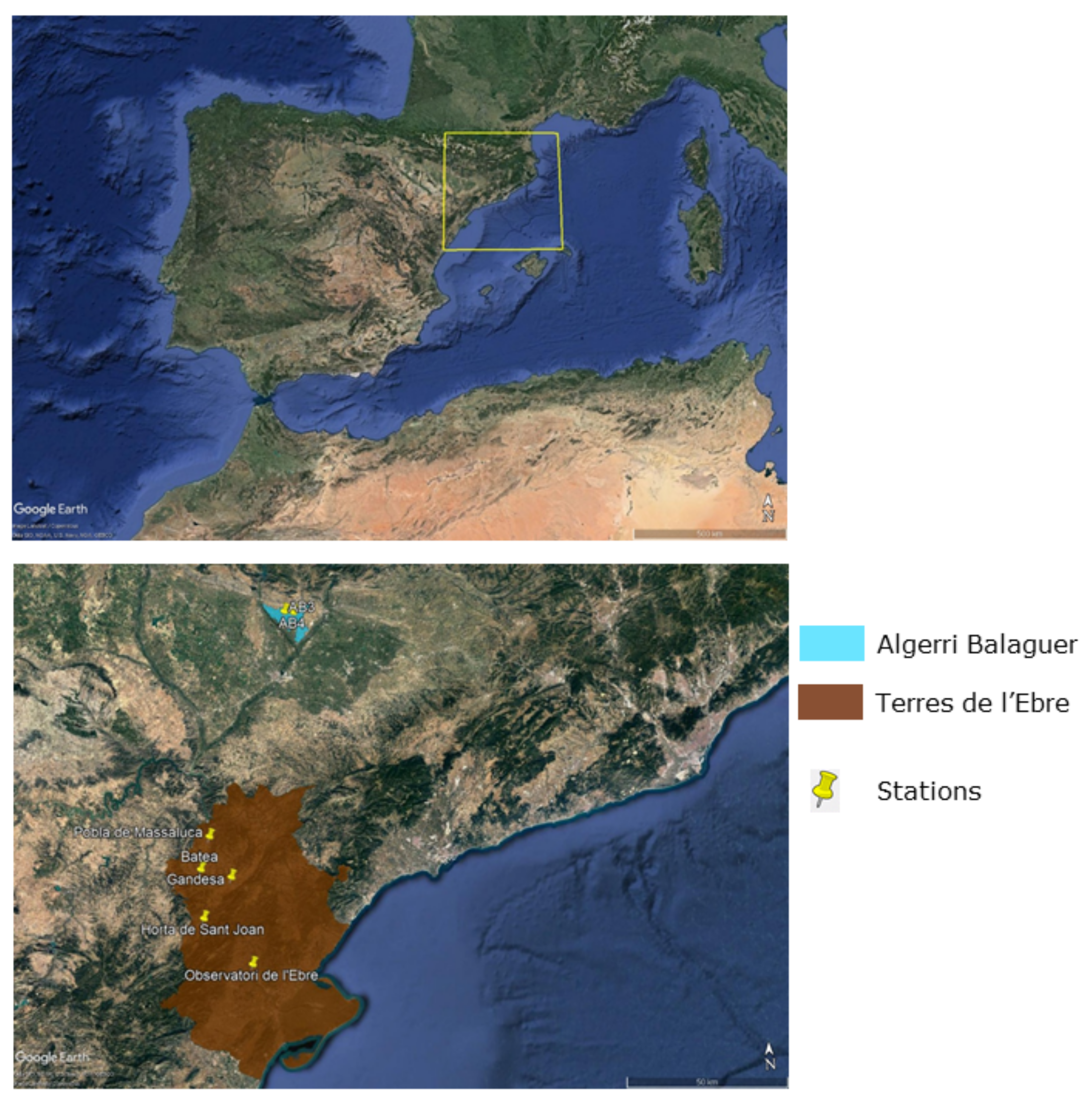
Figure 1. The study area, delimited by a yellow square, located in the NE of the Iberian Peninsula. The Algerri Balaguer and Terres de l’Ebre focus areas are presented in the bottom picture, along with the in situ stations.
Remotesensing 13 01112 g001
Figure 2. The two-step calibration scheme of τ : (1) τ I S B A and (2) τ L C .
Remotesensing 13 01112 g002
Figure 3. (a) 1 km resolution map of ESA CCI reduced land cover, (b) 1 km resolution map of τ L C values.
Remotesensing 13 01112 g003
Figure 4. Boxplots of τ L C values.
Remotesensing 13 01112 g004
Figure 5. 1 km resolution ESA CCI reduced land cover zoomed over the validation areas: (a) Terres de l’Ebre and (b) Algerri Balaguer. The location of the validation sites are represented by circles.
Remotesensing 13 01112 g005
Figure 6. Time series of scaled in situ and SMAP-derived 1km resolution RZSM and SSM estimates. The images refer to data collected over the Terres de l’Ebre region in the following order: BA, GA, HA1, HA2, PM and OE.
Remotesensing 13 01112 g006
Figure 7. Time series of scaled in situ and SMAP-derived 1km resolution RZSM and SSM estimates. The images refer to data collected over the Algerri Balaguer region in the following order: AB3_2017, AB3_2018, AB3_2020, AB4_2017, AB4_2018, AB4_2019.
Remotesensing 13 01112 g007
Figure 8. Map of land use over the Algerri Balaguer area.
Remotesensing 13 01112 g008
Figure 9. Evolution of the NS score at different depths with respect to τ values for Terres de l’Ebre.
Remotesensing 13 01112 g009
Figure 10. Evolution of the correlation at different depths with respect to τ values for Terres de l’Ebre.
Remotesensing 13 01112 g010
Table 1. Correlation coefficient (R), root mean square error (RMSE), bias, slope of the linear regression and Nash–Sutcliffe efficiency score between SMAP-derived 1 km RZSM (with τ L C ) and scaled in situ measurements over Terres de l’Ebre. In parentheses, for comparison purposes, the same statistical results are presented, but taking into account τ I S B A .
SiteDepth (cm)RRMSEBiasSlopeNS
BA700.640.330.1190.170.16
(0.64)(0.33)(0.119)(0.17)(0.16)
500.650.260.0160.200.31
(0.65)(0.26)(0.016)(0.20)(0.31)
250.710.210.0010.260.39
(0.71)(0.20)(0.001)(0.26)(0.39)
100.760.16−0.0580.350.41
(0.76)(0.16)(−0.058)(0.35)(0.41)
50.770.17−0.0470.340.44
(0.75)(0.17)(−0.047)(0.34)(0.44)
GA700.540.28−0.1120.250.16
(0.54)(0.28)(−0.112)(0.25)(0.16)
500.750.280.0010.310.45
(0.75)(0.28)(0.001)(0.31)(0.45)
250.840.250.0630.370.51
(0.84)(0.25)(0.063)(0.37)(0.51)
100.790.18−0.1140.520.33
(0.79)(0.18)(−0.114)(0.52)(0.33)
50.830.18−0.1250.530.35
(0.83)(0.18)(−0.125)(0.53)(0.35)
HA1700.640.290.0460.280.36
(0.64)(0.29)(0.046)(0.28)(0.36)
500.710.240.0250.350.45
(0.71)(0.24)(0.025)(0.35)(0.45)
250.710.240.0510.350.43
(0.71)(0.24)(0.051)(0.35)(0.43)
100.800.190.0610.440.54
(0.80)(0.19)(0.061)(0.44)(0.54)
50.800.190.0760.470.52
(0.80)(0.19)(0.076)(0.47)(0.52)
HA2700.620.32−0.0240.250.34
(0.62)(0.32)(−0.024)(0.25)(0.34)
500.710.26−0.0940.350.37
(0.71)(0.26)(−0.094)(0.35)(0.37)
250.790.21−0.1110.450.42
(0.79)(0.21)(−0.111)(0.45)(0.42)
100.810.17−0.0920.540.49
(0.81)(0.17)(−0.092)(0.54)(0.49)
50.840.17−0.0060.480.63
(0.84)(0.17)(−0.006)(0.48)(0.63)
PM700.380.27−0.1200.20−0.08
(0.39)(0.27)(−0.072)(0.20)(−0.06)
500.700.18−0.0480.380.42
(0.71)(0.18)(−0.048)(0.38)(0.43)
250.820.180.0290.410.56
(0.83)(0.18)(0.029)(0.41)(0.56)
100.830.170.0020.420.58
(0.83)(0.17)(0.003)(0.42)(0.59)
50.840.15−0.0100.460.62
(0.85)(0.15)(−0.010)(0.45)(0.62)
OE1000.570.28−0.0030.300.33
(0.55)(0.28)(−0.003)(0.29)(0.30)
500.850.19−0.0900.520.57
(0.84)(0.19)(−0.090)(0.52)(0.56)
250.900.19−0.1550.660.37
(0.89)(0.19)(−0.155)(0.66)(0.37)
100.910.19−0.1490.650.42
(0.91)(0.19)(−0.149)(0.66)(0.43)
50.880.16−0.1060.630.57
(0.88)(0.16)(−0.106)(0.63)(0.58)
Table 2. Same as Table 1, but for Algerri Balaguer.
SiteDepth (cm)RRMSEBiasSlopeNS
AB3_2017500.210.310.1960.05−0.59
(0.21)(0.31)(0.196)(0.05)(−0.59)
250.480.200.0400.140.16
(0.48)(0.20)(0.040)(0.14)(0.16)
50.480.380.3270.14−2.13
(0.48)(0.38)(0.327)(0.14)(−2.13)
AB3_2018500.540.300.2030.18−0.39
(0.54)(0.30)(0.203)(0.18)(−0.39)
250.470.320.2080.15−0.41
(0.47)(0.32)(0.208)(0.15)(−0.41)
50.540.370.2870.17−0.86
(0.54)(0.37)(0.287)(0.17)(−0.86)
AB3_2020500.330.260.2170.11−1.93
(0.33)(0.26)(0.217)(0.11)(−1.93)
25−0.160.370.301−0.04−2.57
(−0.16)(0.37)(0.301)(−0.04)(−2.57)
5−0.010.350.259−0.00−1.31
(−0.01)(0.35)(0.259)(−0.00)(−1.31)
AB4_201750−0.020.320.118−0.00−0.26
(−0.01)(0.32)(0.117)(0.00)(−0.24)
25−0.560.340.101−0.16−0.54
(−0.52)(0.34)(0.100)(−0.16)(−0.54)
5−0.530.330.098−0.16−0.53
(−0.50)(0.33)(0.096)(−0.16)(−0.52)
AB4_2018500.460.280.1480.15−0.13
(0.47)(0.27)(0.147)(0.16)(−0.12)
250.370.19−0.0690.160.01
(0.39)(0.19)(−0.070)(0.17)(0.01)
50.480.210.0690.170.13
(0.51)(0.21)(0.068)(0.19)(0.15)
AB4_2019500.270.21−0.0250.060.06
(0.29)(0.21)(−0.026)(0.08)(0.07)
250.280.24−0.1370.07−0.35
(0.30)(0.24)(−0.137)(0.08)(−0.34)
50.190.270.0080.030.03
(0.20)(0.27)(0.007)(0.04)(0.04)
Publisher’s Note: MDPI stays neutral with regard to jurisdictional claims in published maps and institutional affiliations.