Article

Atmospheric Correction of Satellite Optical Imagery over the Río de la Plata Highly Turbid Waters Using a SWIR-Based Principal Component Decomposition Technique

by
Juan Ignacio Gossn
1,*,
Robert Frouin
2 and
Ana Inés Dogliotti
1
1
Instituto de Astronomía y Física del Espacio (IAFE), CONICET-Universidad de Buenos Aires, Pabellón IAFE, Ciudad Universitaria, Ciudad Autónoma de Buenos Aires C1428ZAA, Argentina
2
Scripps Institution of Oceanography, University of California San Diego, 8622 Kennel Way, La Jolla, CA 92037, USA
*
Author to whom correspondence should be addressed.
Remote Sens. 2021, 13(6), 1050; https://doi.org/10.3390/rs13061050
Submission received: 17 January 2021 / Revised: 22 February 2021 / Accepted: 28 February 2021 / Published: 10 March 2021
(This article belongs to the Special Issue Atmospheric Correction for Remotely Sensed Ocean Color Data)

Abstract

:
Estimating water reflectance accurately from satellite optical data requires implementing an accurate atmospheric correction (AC) scheme, a particularly challenging task over optically complex water bodies, where the signal that comes from the water prevents using the near-infrared (NIR) bands to separate the perturbing atmospheric signal. In the present work, we propose a new AC scheme specially designed for the Río de la Plata—a funnel-shaped estuary in the Argentine–Uruguayan border—highly scattering turbid waters. This new AC scheme uses far shortwave infrared (SWIR) bands but unlike previous algorithms relates the atmospheric signal in the SWIR to the signal in the near-infrared (NIR) and visible (VIS) bands based on the decomposition into principal components of the atmospheric signal. We describe the theoretical basis of the algorithm, analyze the spectral features of the simulated principal components, theoretically address the impact of noise on the results, and perform match-ups exercises using in situ measurements and Moderate Resolution Imaging Spectrometer (MODIS) and Visible Infrared Imaging Radiometer Suite (VIIRS) imagery over the region. Plausible water reflectance retrievals were obtained in the NIR and VIS bands from both simulations and match-ups using field data—with better performance (i.e., lowest errors and offsets, and slopes closest to 1) compared to existing AC schemes implemented in the NASA Data Analysis Software (SeaDAS). Moreover, retrievals over images in the VIS and NIR bands showed low noise, and the correlation was low between aerosol and water reflectance spatial fields.

Graphical Abstract

1. Introduction

In atmospheric correction (AC) of optically complex waters such as the Río de la Plata (RdP), the black water assumption in the near-infrared (NIR) bands on which traditional AC schemes rely [1,2] is usually invalid due to the high backscattering produced by the high concentration of suspended particulate matter (SPM) present in the water [3,4,5]. Furthermore, over RdP, the iterative schemes based on the NIR bands—such as [6,7]—usually do not provide good estimates in Moderate Resolution Imaging Spectrometer (MODIS) images due to either the saturation of NIR bands or limitations in the bio-optical model used to estimate the water reflectance in the NIR and visible (VIS) bands. Although other strategies based on the black water assumption in the shortwave infrared (SWIR) bands have already been proposed [8,9], in this work we explore the possibility of implementing this strategy but with a different extrapolative scheme based on the principal component analysis (PCA) of a set of radiative transfer simulations in which only the atmosphere and the air–water interface effects are considered (i.e., where water reflectance, ρw, is equal to zero). The main difference with existing AC schemes is that the quantities used for extrapolation are obtained from the variance–covariance matrix of the set of simulations and not from non-linear estimators such as the ratio of the signals at the correction bands, ε(λ1, λ2). Other authors such as Gross et al. 2007 [10] have implemented a PCA-based AC, but they used a full-spectrum decomposition on both the atmospheric and water reflectance. This approach imposes spectral constraints on the latter, as other full-spectrum approaches such as POLYMER [11] do. Contrary to this, our scheme does not depend on any assumption on the water reflectance except over the far SWIR where we assume negligible water-leaving radiance. This is considered a robust assumption even for extremely high suspended sediment concentrations, given the very strong absorption of liquid water in these bands, [12,13,14]. Our AC also relies on the assumption of spectral smoothness of the atmospheric (Rayleigh-corrected) reflectance, i.e., a high correlation between the SWIR and NIR atmospheric signals, an assumption that strongly holds, especially at long wavelengths [15,16,17]. Although this AC was intended to be applied to the NIR bands and then be coupled to a conventional extrapolative method from the NIR, in this paper we analyzed the possibility of estimating the water reflectance in the VIS by applying a direct extrapolation from the SWIR to the VIS.
In the present study, the performance of our approach—hereafter referred to as the PCA-SWIR approach—was theoretically tested from a set of radiative transfer simulations combining various atmospheric conditions and in situ measurements of water reflectance collected in the RdP. Additionally, various PCA-SWIR schemes were analyzed using different combinations of far-SWIR bands present in the MODIS, Visible Infrared Imaging Radiometer Suite (VIIRS), and future Satélite Argentino-Brasileño para Información Ambiental del Mar (SABIA-Mar) sensors. The degradation of the AC performance when applied to MODIS/Aqua images due to sensor noise was addressed by a geostatistical approach combined with radiative transfer simulations. The PCA-SWIR AC was then applied to VIIRS and MODIS imagery over RdP and a match-up exercise was performed using in situ data from RdP. Results obtained using the PCA-SWIR13 scheme, i.e., SWIR bands tagged as 1 and 3, were compared to other existing ACs. Finally, a spatial analysis of the retrieved aerosol and water reflectance was performed using different ACs.

2. Materials and Methods

2.1. Algorithm Description

The PCA-SWIR AC starts from assuming a negligible contribution of the water-leaving radiance over the total radiance budget received by the satellite sensor at top-of-atmosphere (TOA) in the SWIR bands and assuming a high correlation of the aerosol signal between the SWIR bands and the VIS/NIR bands. Consider the following expression for the Rayleigh-corrected (RC) reflectance at top-of-atmosphere (TOA),   ρ RC , [1]:
ρ RC = ρ a + T ρ g + t ρ w ,
where ρa, Tρg, and tρw are the aerosol, glint, and water reflectance contributions at TOA, and T and t are the direct and total (direct + diffuse) transmittance factors, respectively. In this equation, ρ RC is defined as π L RC / [ F 0 cos ( θ s ) ] where L RC is the respective Rayleigh-corrected radiance, F 0 the extra-terrestrial solar irradiance, and θ s the solar zenith angle, and ρ w is defined as π L w / E d where L w is the water-leaving radiance and E d the downwelling solar irradiance just above the surface. Assuming that the water reflectance in the SWIR is negligible (the so-called black pixel assumption) and selecting regions that are not affected by direct sun glint, the RC reflectance in the SWIR and VIS–NIR bands (subscript “VN”) can be expressed as:
ρ RC ( λ SWIR )     ρ a (   λ SWIR ) ,
ρ RC ( λ VN ) ρ a ( λ VN ) + t ( λ VN ) ρ w ( λ VN ) .
We propose to model the aerosol term as a combination of principal components of a set of radiative transfer simulations in which the water reflectance is set to zero (ρw = 0) (see Section 2.2). The principal components correspond as usual to an orthogonal basis of eigenvectors of the variance–covariance matrix of the set of simulated RC reflectance values. Assuming that most of the explained variance is expected to be contained in the first two or three principal components, the aerosol reflectance in the VIS/NIR bands, ρaVN), can be obtained as:
ρ a ( λ VN )     a 1 e 1 , VN PCA + a 2 e 2 , VN PCA + ρ a ( λ VN ) ,
where e j , VN PCA represents the VN component of the j-th principal component of the set of simulations, a1 and a2 represent the projections of the first N components, and <⬝> represents the mean value of the aforementioned ensemble of simulations.
Notice that the total number of eigenvectors is N + 1, i.e., the number of SWIR bands (N = 2 or N = 3 depending on the scheme) plus the VIS/NIR band to be corrected, meaning that the last principal component is assumed to have negligible contribution to the aerosol signal in Equation (4). Given that the N first components explain >95% of the variance in the considered set of simulations (see Section 4.1.1), this assumption is considered as reasonable. The projections of the N first principal components (hereafter N = 2 for brevity), a1 and a2, can then be obtained by inverting the linear system composed of Equation (2) specified at the two SWIR bands and assuming the same decomposition as in Equation (4):
( e 1 , SWIR 1 PCA e 2 , SWIR 1 PCA e 1 , SWIR 2 PCA e 2 , SWIR 2 PCA ) ( a 1 a 2 ) = ( ρ RC ( λ SWIR 1 ) ρ RC ( λ SWIR 2 ) ) - ( RC ( λ SWIR 1 ) ρ RC ( λ SWIR 2 ) ) .
The N × N matrix (2 × 2 in this example) that appears on the left hand side of Equation (5) is a subset of the variance–covariance matrix of size (N + 1) × (N + 1) and is the fundamental matrix of the scheme, herein M, being M j , λ =   e j , λ PCA (j = 1,…,N, and λ = SWIR1,…,SWIR-N). Any error in the right-hand side of Equation (5) (sensor noise, calibration error, or error introduced in the obtention of ρ RC ), is potentially amplified by the linear inversion and the bound to such error amplification is measured by the condition number of M:
Cond ( M )   =   M M 1 ,
where M = max x 0 { M . x 2 x 2 } , being x an N-tuple and · 2 the conventional Euclidean norm.
Once a1 and a2 are obtained from Equation (5), they are replaced in Equation (4) and the aerosol reflectance at the band of interest, ρ a ( λ VN ) , is subtracted from the Rayleigh-corrected signal, leaving the term t(λVNwVN) in Equation (3). Finally, the water reflectance is obtained using the following simplified expression to calculate the total transmittance, t(λVN), proposed by Tanré et al., 1979 [18]:
t ( λ ) = e - ( 1 2 τ r ( λ ) + 1 6 τ a ( λ ) ) . m .
where m = sec(θs) + sec(θv) is the air mass factor and where an average anisotropy factor of ⅔ is assumed for aerosols. To estimate the transmittance factor, the following aerosol optical thickness τa(λ) was used:
τ a ( λ ) = 0 . 06 ( λ 500   nm ) - 1 .
This expression is a power law where the Angstrom exponent is fixed at 1, as in Steinmetz et al., 2011 [11], and the value at τa(500 nm) = 0.06 corresponds to the mode of the set of values measured at the CEILAP-BA AERONET station located in Buenos Aires (approximately 3 km from RdP northwest coast). Naturally, the anisotropy factor and the aerosol optical thickness are not fixed in nature, but this simplified expression for the transmittance is preferred in this work given that the focus is on the PCA extrapolation procedure and the fact that the approximations used to obtain the transmittance factor typically have a low impact over the total error budget of the AC in comparison to other sources of error. It must be reinforced that these constraints are posed only over the transmittance factor (a second order correction factor) and not over the set of simulations from which e j , λ PCA is derived. Figure 1 schematizes the steps performed to calibrate the algorithm and to apply it to both images and simulated data.

2.2. Radiative Transfer Simulations

To simulate the top-of-atmosphere (TOA) reflectance in the spectral bands of the sensors listed in Table 1, the Centre National d’Études Spatiales/Successive Orders of Scattering (CNES-SOS) radiation transfer code v5.0 [19,20] was used to produce two sets of simulations:
Set 0: This set was used to calibrate the principal components of the atmospheric signal, i.e., the eigenvectors of the variance–covariance matrix of the set in the VIS/NIR/SWIR bands. It was composed of CNES-SOS simulations with null water reflectance (ρw = 0).
Set W: This set was used to theoretically evaluate the performance of the AC in the VIS/NIR bands. It was composed of CNES-SOS simulations where a subset of 22 water reflectance spectra measured with an Analytic Spectral Device (ASD) was used as input instead of the black water condition of Set 0 (Figure 2). The inclusion of water reflectance to the CNES-SOS code is done through the addition of a Lambertian (isotropic non-polarized) term in the surface Mueller matrix, which also contains the Fresnel reflectance term (for further detail see [19]). This subset of 22 measurements was selected in order to span a large range of measured water reflectance in the RdP with a pseudo-uniform step, i.e., trying to cover in the most uniform possible way all the range of water reflectance values that were measured in the region of interest in order to avoid sampling biases in the retrievals. The reflectance in each band of interest (Table 1) was calculated using the spectral response functions (SRFs) that are available from the NASA Ocean Biology Processing Group (OBPG) webpage [21] in the cases of MODIS and VIIRS, and using square-shaped SRFs defined by the centers and bandwidths reported by CONAE in the case of the SABIA-Mar sensor (Dr. Carolina Tauro, Principal Investigator of the SABIA-Mar mission, personal communication).
The remaining parameters used as input to CNES-SOS are detailed in Table 2. The Rayleigh scattering due to air molecules was parameterized following the optical thicknesses and molecular depolarization ratio reported by Bodhaine et al., 1999 [22], using an e-folding molecular height scale of 8 km, i.e., assuming an isothermal-barotropic atmosphere. The aerosol physical properties, characterized by their granulometry and complex refractive index, were parameterized assigning linear combinations of the continental, maritime, and urban scenarios proposed by the World Meteorological Organization [23]. Assuming no prior information regarding aerosol type, we considered equally all the 15 combinations produced by combining these three types of scenarios in quarters, e.g., maritime 25%, continental 25%, urban 50%, or maritime 25%, continental 75%, urban 0%. An e-folding height scale of 2 km was assumed for aerosols. Their concentrations were parameterized by the aerosol optical thickness at surface and at a reference wavelength of 500 nm, τa(500 nm), log-normally distributed with a mode of 0.06, determined from sun-photometric measurements made at the CEILAP-BA AERONET station in the 1999–2013 period [24]. The range of surface wind speeds (used by the SOS code to calculate surface roughness) was selected based on the wind measurements at the Aeroparque Meteorological Station—located just by the RdP river in the city of Buenos Aires—for the period 1976–2014. The values of 0, 2, 4, 8, and 16 m/s were chosen, geometrically distributed, given that the most probable wind speeds were within the range of 4 to 6 m/s, and winds greater than 14 m/s were recorded in much less than 1% of the measurements. In the simulations, the effect of whitecaps was not considered, given their negligible contribution in the highly reflective waters of interest in this study.
Rayleigh correction was performed over both sets of TOA simulations (Sets 0 and W) before computing the associated eigenvectors to Set 0 and applying the PCA scheme to Set W. To achieve this, the code was run twice for each subset to compute the TOA reflectance ( ρ TOA SOS ) with two conditions: (i) using the input values specified by Table 2, and (ii) assuming a black marine environment (ρw = 0) and no aerosol content (τa = 0). The results from (ii) were subtracted from those from (i) to yield the RC signal, both in Sets 0 and W:
ρ RC SOS = ρ TOA SOS [ Air + Aerosols + Surf + Water ]   -   ρ TOA SOS [ Air + Surf ] ,
where Surf stands for the air–water interface. To prevent an overrepresentation of sun glint on the PCA eigenvectors, we discarded the subset of sun-observation geometries and wind speed combinations—in both Sets 0 and W—where the reflectance due to sun glint exceeded the threshold of 0.005. To perform this pre-selection, the sun glint reflectance, ρg, was computed separately by generating a set of simulations with null water-leaving radiance reflectance and no atmosphere (ρw = 0 and τr = τa = 0).
The PCA-SWIR AC over the simulated RC reflectance ensemble (Set W) was applied using the four possible SWIR band combinations (see Table 1), i.e., PCA-SWIR12 when using SWIR bands 1 and 2, and the same for PCA-SWIR13, PCA-SWIR23, and PCA-SWIR123.

2.3. Other AC Algorithms and Match-up Procedure

We applied the PCA-SWIR scheme and other existing ACs on MODIS (onboard Aqua and Terra) and VIIRS (onboard Suomi-NPP and NOAA20 platforms) imagery over RdP for the dates when field measurements were collected within the period 2012–2020 (Section 3.1). Even though we tested all the four possible PCA-SWIR schemes over the imagery, in the current paper we only show the global intercomparison between existing ACs and PCA-SWIR13, since this is the only option that does not make use of the band SWIR2, which is no longer operational in MODIS/Aqua. Apart from PCA-SWIR13, the following ACs implemented in the SeaDAS/L2Gen ocean color Level2 processor [21] were also applied and considered in the match-up exercise (also summarized in Table 3):
  • NIR multi-scattering extrapolative approach (GW94-NIR): This AC was proposed by Gordon and Wang 1994 [1] and computes the aerosol signal accounting for multiple scattering effects and assuming black water in the NIR. It was the standard AC implemented for Sea-viewing Wide Field-of-View Sensor (SeaWIFS) imagery and is suitable for open waters;
  • Iterative scheme in the NIR (ITER-NIR): This AC is based on an iterative procedure to subtract the non-zero contribution of the water to the NIR signal based on a convergence strategy and on a semi-empirical model for the water reflectance in the NIR and VIS. It is described in [6,7]. This AC has been shown to underestimate water reflectance and even fail to produce any retrieval in RdP’s maximum turbidity front [5,17], but it is considered here because it is the standard AC implemented by L2Gen in SeaDAS;
  • SWIR multi-scattering extrapolative approach (GW94-SWIR): This AC computes the aerosol signal accounting for multiple scattering effects and assuming black water in two specified bands in the SWIR. It is similar to the Gordon and Wang 1994 [1] approach, except it is adapted to SWIR bands [4,5,8];
  • Rayleigh correction scheme (RC): This AC only removes the effect of Rayleigh scattering and molecular absorption, i.e., it does not correct the contribution of aerosols to the TOA reflectance. This AC was considered because it is reasonable to test the extent to which an aerosol correction is necessary over the RdP’s highly reflective waters.
All the aforementioned ACs were run without applying the bidirectional reflectance distribution function (BRDF) correction (brdf_opt = 0), which accounts for the directionality of the upwelling radiance. This correction was not applied given that it generally degrades performance in turbid waters [25]. The gaseous absorption correction was set to account for ozone, carbon dioxide, nitrogen dioxide, and water vapor (gas_opt = 15). The land and clouds were masked (using a cloud threshold of 0.018 at the SWIR3 band) as well as pixels with high sun zenith angle (θs > 60°) and view zenith angle (θv > 70°). The sun glint mask was not applied (to eventually test the robustness of the PCA-SWIR schemes in sun glint conditions). Additionally, the HILT and STRAYLIGHT standard masks were switched off since they usually mask turbid water pixels erroneously. The spatial resolution was fixed at 1000 m.
For every VIIRS and MODIS scene that corresponded to a quasi-simultaneous field measurement (a maximum time difference of 30 min was considered), a window of 3 × 3 pixels was extracted, with its central pixel the closest to the reported coordinates of the field data. In the case of the coastal site at Buenos Aires located at the end of a 500 m long pier (black dot in Figure 3), the window was intentionally shifted away from land (1 pixel North, 1 pixel East in sensor geometry) to reduce the impact of land on the window.
Once the window was selected, a filtering protocol was performed on a band-by-band basis:
  • If the number of AC-failure pixels (i.e., with NaN) was more than 4 out of 9 (>44.4%), the window was discarded (no match-up). Otherwise, the median and the standard deviation of the remaining pixels were taken as the reported value (x) and the absolute error (ux) of the window, respectively;
  • If the coefficient of variation (CV = ux/x) exceeded 20% at a given band, the station was discarded (no match-up).

2.4. Evaluation Metrics

To analyze the performance of the ACs, linear regressions between predicted (remotely estimated or simulated) and observed (in situ) reflectance were performed using a Theil–Sen linear regressor [26,27], which is less affected by outliers than least-squares regressors. From these regressions the usual linear regression statistics were obtained, i.e., slope, offset, and coefficient of determination R2. For the match-up exercise, the root mean square error (RMSE), the mean absolute difference (MAD), the mean difference (MD) and the mean absolute percentage difference (MAPD) were also computed as follows:
RMSE = 1 N m i = 1 N m ( ρ w , i sat - ρ w , i field ) 2 ,
MAD = 1 N m i = 1 N m | ρ w , i sat - ρ w , i field | ,
MAPD = 100 % × 1 N m i = 1 N m | ρ w , i sat - ρ w , i field ρ w , i field | ,
MD = 1 N m i = 1 N m ( ρ w , i sat - ρ w , i field ) ,
where the subscript i accounts for each individual match-up, and Nm is the total number of match-ups. Given that the selection criteria mentioned in Section 2.3 might yield different Nm values for different ACs, the absence of effective retrieval in the computation of the absolute statistics (i.e., RMSE, MAD, and MAPD) was penalized in the following way: when the i-th station for a given AC was missing, its value was replaced by the worst value retrieved by the remaining ACs in the absolute sense (i.e., the one with highest |ρw,isatw,ifield|). This was done to minimize biases caused by different Nm among ACs. The total number of real match-ups, Nm, will also be shown as a general indicator of performance of the ACs.

3. Field Data

3.1. Study Area

The Río de la Plata (RdP) is a funnel-shaped estuary located at Eastern-Central South America (Figure 3) and drains the second largest basin in South America, transporting between 80 and 160 million tons of sediments every year. Several measurements of suspended particulate matter (SPM) concentration were taken during field campaigns over the period 2012–2020, with values varying from 4.38 g/m3 to 940.00 g/m3 (median: 61.40 g/m3, interquartile range: 48.56 g/m3). The RdP has a stationary maximum turbidity front associated with a saline front where the fresh waters of the estuary meet the South Atlantic salty waters [28,29]. The position of this front is mainly controlled by the bathymetry and coincides with the “La Barra del Indio” shoal in the north sector and with the 5 m isobath in the Samborombón Bay to the south. The RdP transports large amounts of sediments whose behavior is relevant for a number of applications in coastal areas. Several studies that make use of ocean color imagery have been conducted to determine the area of influence of the Rio de la Plata turbid plume over coastal waters of the Southwest Atlantic adjacent to the estuary [30,31,32,33]. The high-SPM and highly reflective waters of RdP and its extension (42 km to 220 km wide and 275 km long) make the estuary an excellent site to test ACs over moderate resolution ocean color radiometers such as MODIS and VIIRS.

3.2. Radiometric Measurements

A total of 55 in situ above-surface radiometric measurements collected during several field campaigns between 2012 and 2020 in the RdP (Figure 2a) were used both as input to radiative transfer simulations to theoretically test the PCA-SWIR AC and to perform match-ups with satellite data. From these 55 measurements, made over waters with SPM concentration ranging between 6 g/m3 and 522 g/m3 and nephelometric turbidity between 9 FNU and 708 FNU (measured using a portable HACH 2100P ISO), 28 were acquired using a set of three RAMSES/TriOS hyperspectral spectroradiometers (spectral range 350 nm to 950 nm, spectral resolution 3.3 nm, spectral discretization 2.5 nm), two measuring upwelling and downwelling radiances just above surface (L0+u and L0+d, respectively) at a relative azimuth angle from the sun of either 135° or 90° and reciprocal zenithal angles of θ = ±40°, respectively, and one pointing toward zenith to measure downwelling irradiance, E0+d. The remaining 27 measurements were acquired with an Analytic Spectral Device (ASD FieldSpec FR) spectroradiometer (spectral range 350 nm to 2500 nm, spectral resolution 3 nm between 350 nm and 900 nm and of 10 nm to 12 nm in the range 900 nm to 2500 nm, with a spectral discretization of 1 nm) that consisted of a single radiometer connected to an optical fiber of 8° aperture that was sequentially pointed to water and sky to determine L0+d and L0+u using the same sun-viewing geometry as with TriOS and pointed to a quasi-Lambertian Spectralon plaque to determine E0+d by multiplying the nadir radiance leaving the plaque by π. The reflectance of the plaque (>0.99 in the range 400–1500 nm) was assumed equal to 1. These measurements were combined to calculate the water reflectance ρw according to
ρ w ( λ ) = π ( L u 0 + ( λ ) - ρ M ( W ) L d 0 + ( λ ) ) E d 0 + ( λ ) ,
where ρM(W) is the surface radiance reflectance factor taken from Mobley 1999 [34], which depends on the wind speed, W. Since many of these measurements were taken at coastal sites or close to the coast, the relation between the surface roughness and the wind speed used to parametrize the surface radiance reflectance in Mobley 1999 no longer holds. In those cases, we fixed ρM at 0.0256, i.e., at null wind speed. The protocols used with both radiometers followed the generic “Above-water Method 2” of the NASA 2003 Ocean Optics Protocols (Mueller et al., 2003 [35]) and followed the recommendations issued by Ruddick et al., 2019 [36,37]. The details of the measurement protocols are described by Knaeps et al., 2012 [38] for ASD and Tilstone et al., 2001 [39] for TriOS and are thoroughly described in Gossn 2020 [40].

4. Results

4.1. Theoretical Performance

4.1.1. PCA Eigenvectors

The results presented in this and in several of the following sections vary slightly among the considered sensors, so they will not be shown for all of them. A set of PCA eigenvectors is displayed in Figure 4, calculated from SOS simulations (Set 0) in different bands/sensors for the model that used VIIRS 1241 nm, 1602 nm, and 2257 nm SWIR bands (PCA-SWIR123). Note that the eigenvectors have dimension N + 1, with N equal to the number of correction bands used in the corresponding model.
Similar to what was shown by Gross et al., 2007 [10], the first PCA eigenvector has a smooth spectral shape, showing that the magnitude—spectrally close to white—of the signal is the first cause of variability between different spectra. This eigenvector is mainly representing the different concentrations of aerosols and the residual component of the water surface Fresnel reflection, strongly dependent on the geometry of observation-illumination and the surface wind. The second eigenvector has a blue signature, which is mainly due to multiple Rayleigh-aerosol scattering, ρra, highly variable depending on aerosol type, and more effective in the blue due to a larger Rayleigh optical thickness in that range. The third and fourth eigenvectors are associated with very small (<5% in the blue and <2% in the NIR) fractions of explained variance and represent high-order departures from the spectral shape of the main principal components. Even though they are not easily interpretable in basic physical terms, their marked spectral features suggest they are associated to the only physical component of our system whose spectral shape varies, i.e., aerosols (either through differential granulometry or chemical composition). As expected, the first two eigenvectors are associated with more than 95% of the variance, as is shown in Table 4. As an example, Table 5 shows the components of the eigenvectors of the PCA-SWIR13 AC scheme for sensors MODIS/Aqua and VIIRS/Suomi-NPP.
The error amplification factors, i.e., the conditional numbers (Equation (6)) of the inversion matrices (left-hand side of Equation (5)) of each scheme, are reported for each band in Table 4. Large numbers are associated with matrices closer to non-invertibility and also with weaker error bounds after inversion (i.e., potentially larger error amplification). This means that the PCA-SWIR123 scheme, given the high conditional numbers in the blue (389.3 vs. 4.8), is likely to produce worse retrievals when compared to the two-SWIR-band schemes, even if the total variance explained by the total used N components is higher in the PCA-SWIR123 case (99.43 vs. 95.42).

4.1.2. Aerosol Signal Estimation (SOS Set 0: Black Water)

The aerosol reflectance retrieved by the PCA-SWIR12 AC applied to the SABIA-Mar BLUE and NIR1 bands in the conditions used to generate the PCA eigenvectors (Set 0), ρ a PCA , is displayed in Figure 5. This exercise allows a first evaluation of the aerosol reflectance estimation prior to the diffuse transmittance correction. In concomitance with what has been discussed in the previous sections, the performance is markedly worse in the BLUE than in the NIR due to a higher spectral distance to the SWIR spectral region. It must be noticed that the PCA-SWIR12 scheme was implemented—with no intermediate steps involving the NIR bands—to estimate ρ a PCA ( 412   nm ) .
In the case of VIIRS bands (Figure 6 and Figure 7), a better performance is observed with PCA-SWIR123 in the NIR when compared to two-band models (slope closer to 1 and lower MAD). On the contrary, we observe worse retrievals in the blue, i.e., for ρa(489 nm), using the three-band model. This is also evident from an abrupt increase in the conditional number of the inversion matrix, as the band to be corrected is spectrally further away from the SWIR bands. The larger conditional number in the blue than in the NIR occurs for all models (both with N = 2 and N = 3, although markedly larger in the latter case (see Table 4), indicating that the inversion matrix of the system of Equation (5) is closer to non-invertibility, which in turn is associated with a low correlation between the bands in the blue and those in the SWIR. It may be seen as counter-intuitive that adding information (i.e., adding a band) can degrade the performance of the algorithm, but it must be emphasized that this only occurs in the blue bands where the correlation to the SWIR is lower than at higher wavelengths. In the case of the model with three corrective bands, this lack of correlation and the addition of a component leads to an overrepresentation of the variability of the reflectance in the blue, implying larger propagation errors.

4.1.3. NIR Water Reflectance Retrieval (SOS Set W)

The retrieved (PCA-SWIR) vs. observed (ASD) water reflectance values in the SABIA-Mar and VIIRS NIR bands are shown in Figure 8 and Figure 9 using all the PCA-SWIR possible combinations of SWIR bands, i.e., one in the case of SABIA-Mar (lacking the SWIR3 band) and four in the case of VIIRS. The results obtained for each of the 22 field reflectance measurements used in the computation of Set W are displayed as the mean values of retrieved ρwPCA (red dots) and the interquartile ranges (IQRs) are represented with red vertical bars. In general, a good correspondence is observed between the estimated and measured reflectance values, with low biases and slopes and correlation coefficients close to 1. Similarly to what was found for the estimates of the aerosol reflectance using the simulations of Set 0, Figure 9 shows that the three-band model presents lower IQRs, i.e., less sensitivity to atmospheric variability, and slopes closer to 1 compared to the two-band schemes.

4.1.4. Effect of Noise on MODIS/Aqua Imagery

In order to study the impact of noise on the performance of the PCA-SWIR scheme, we estimated a noise-equivalent RC reflectance (NEρRC) from MODIS/Aqua imagery. We decided not to use the classic homogeneous area approach of Duggin et al., 1985 [41] given that it supposes a homogeneous “real” field (the field at zero noise) in the selected area, a condition that is never met in the Río de la Plata at the VIS/NIR bands. Instead, we implemented a geostatistical method, which was first applied to satellite (AVIRIS) images by Curran and Dungan 1989 [42]. This method assumes a Gaussian noise model, a null autocorrelation of the noise field, and a null correlation between the noise and the “real” field. After having verified the geostatistical method on synthetic images of known noise, it was applied to a set of RC reflectance rasters (L2 product ρs using SeaDAS v7.5) of 20 MODIS/Aqua images of the Río de la Plata over the period 2013–2019 over a small subregion between 35.26°S and 35.52°S and between 57.05°W and 56.70°W (windows of 40 × 40 pixels approximately, see Figure 3).
Taking the mean of the noise amplitudes in each of the selected subscenes described in the Methods section, the absolute value of the noise, σ, was obtained (Table 6) by estimating the nugget of the associated semi-variogram of each subscene, following [42]. These values were used to theoretically evaluate the impact of noise on the AC performance on MODIS/Aqua. It was assumed that the noise in the individual bands was not correlated spectrally.
The effect of noise in the MODIS/Aqua bands on the performance metrics of the PCA-SWIR algorithm over the set of radiative transfer simulations was found to be low, if taking into account the low signal-to-noise ratios of the SWIR bands (Table 7).
It should be noted that, as already known, a normally distributed noise—of mean 0—is propagated through a linear system into a normally distributed noise—of mean 0—of the retrieved quantity, with the amplification of the noise regulated by the conditional number of the inversion matrix of the scheme. In our case, the output quantity is the aerosol—and eventually, the water—reflectance in the NIR bands. We consider this method to be more robust statistically under the effect of noise in comparison to the standard procedure of using ratios such as ε(λ1, λ2), given that ratios of variables with normally distributed errors are prone to magnifying the effect of noise over the outputs (especially under low mean values of the denominator, i.e., under clear atmospheric conditions). This will be also discussed in the following section.

4.2. Application to Satellite Imagery

4.2.1. Match-ups

The global scatterplots of the match-up exercise are shown for the NIR1 ~750 nm (Figure 10) and NIR2 ~860 nm (Figure 11) bands of all the sensors, and the global performance metrics are shown in Table 8. We decided not to differentiate TriOS and ASD field reflectance measurements graphically since no systematic bias was observed between them. Inside each inset, the satellite-derived water reflectance (ρwsat) was compared with the field-measured water reflectance ( ρ w field ) for ITER-NIR, RC, GW94-SWIR13 and PCA-SWIR13 in the NIR bands) (see Table 3 for a description of these acronyms). It should be noticed that different total numbers of effective match-ups are obtained for each AC given the different AC failure and acceptance ratios after following the quality control criteria described in Section 2.3. The NIR-iterative (ITER-NIR, a) and standard NIR-black-water (GW94-NIR, b) ACs tend to underestimate water reflectance at all wavelengths and especially at high field-reflectance values, frequently failing to retrieve numerical values (seen as lower N values) or otherwise retrieving negative reflectance.
On the other hand, even if the results of the PCA-SWIR13 scheme in the blue and green show general overestimation (MD = 0.019 and MD = 0.011, respectively, see Table 8), they still show better agreement with field data in comparison with those of the GW94-SWIR13 approach (slopes closer to 1, less negative retrievals, and higher N—i.e., fewer AC failures).
In the NIR bands, the Rayleigh correction approach (RC, Figure 10b and Figure 11b) tends to overestimate water reflectance (with intercepts of 0.012 and 0.014 and MD of 0.0103 and 0.0103 in bands NIR1 and NIR2, respectively) in comparison with the other schemes, all of which intend to remove the aerosol effect. The PCA-SWIR13 AC clearly shows an improved performance over the standard NIR procedures. When compared to GW94-SWIR13, a slightly better performance is attained in the NIR1 band—considering the obtained RMSE, MAD, MD, MAPD, slope, and R2, and a clear improvement is observed in the NIR2 band, with retrieved slope and R2 close to 1 and RMSE, MAD, MAPD, and MD closer to 0.
A subset of field water reflectance spectra together with the corresponding satellite-derived reflectance spectra from sensors MODIS/Terra (MT) and VIIRS/Suomi-NPP (VSNPP) is shown in Figure 12. These examples show general agreement in spectral magnitude and shape between field and PCA-SWIR13 spectra, with a tendency to achieve better performance in the green-red-NIR region of the spectrum when compared to ITER-NIR, GW-NIR, and GW-SWIR13 ACs. In the blue region, even though the PCA-SWIR13 scheme comparatively performs better than the other schemes, with fewer AC failures and negative retrievals, it tends to overestimate reflectance in the blue. This overestimation may be associated with a magnification of the error produced by higher condition numbers of inversion (Equation (6)) and the simple model of the diffuse transmittance factor expressed in Equation (7) (see Discussion section).

4.2.2. Spatial Analysis of Water and Aerosol Patterns

Another way of evaluating the quality of an AC is to compare the spatial patterns of the water and aerosol reflectance. If the algorithm is capable of decoupling both signals spectrally on a pixel-by-pixel basis, it is also expected that it will do so spatially, even though water properties/processes may partly affect local aerosol production. When comparing the performance of PCA-SWIR13 with other ACs (Table 3), we found lower spatial correlations and lower percentages of AC failures and negative water reflectance pixels, as well as less noisy aerosol retrievals in the VIS/NIR with the PCA-SWIR13 AC. This is exemplified in Figure 13 and Figure 14, which display the water and aerosol reflectance maps produced for the MODIS/Aqua scene of 2014-05-16T17:35:00Z using the PCA-SWIR13, GW94-NIR, ITER-NIR, and GW94-SWIR13 ACs in the blue (443 nm) and NIR2 (859 nm) bands, respectively. In both bands, the PCA-SWIR13 AC yields the least cross-contamination of the water and aerosol reflectance, fewer AC failures (shown in white), negative reflectance pixels, and lower slopes on the ρa vs. ρw relation. Even though a lower slope is observed for GW94-SWIR13 than for PCA-SWIR13 at 443 nm, this may be associated with the much shorter range of retrieved water reflectance. In general, the performance is markedly improved when compared to standard NIR approaches (GW94-NIR and ITER-NIR). Note that the GW94-NIR AC is not shown in Figure 14 because this scheme retrieves trivially zero water reflectance in the NIR bands. When comparing PCA-SWIR13 with GW94-SWIR13, the slightly lower slope on ρa vs. ρw indicates that in the selected region (shown inside squared contours), where the maximum turbidity front of Río de la Plata is located [43], there is a slightly better water reflectance estimation. Additionally, a markedly lower percentage of negative reflectance pixels (0.00% vs. 7.11% in the BLUE band; 1.26% vs. 5.72% in the NIR2 band), lower percentage of AC failures (0.45% vs. 2.31% in the blue band; 0.45% vs. 0.71% in the NIR2 band) is observed. It is worth noting that PCA-SWIR13 aerosol reflectance maps are less noisy compared to the traditional extrapolative approach (compare insets (c) and (f) in both figures).

5. Discussion

The new AC presented here has multiple advantages. First of all, it relies on simple and plausible physical hypotheses which, given the simplicity of the algorithm, can be tracked and tested with ease. It also has the advantage that the generalization of the inversion procedure to the use of multiple sets of SWIR correction bands is straightforward, which is not the case of standard extrapolative procedures that rely on ratios over pairs of bands. Additionally, given the linear nature of the inversion scheme, this AC keeps the structure of the noise and also tends to bound the noise better than in the case of band ratios. This is a key point, since ratios of normally distributed random variables (i.e., assuming a Gaussian noise model), such as ε(λ1, λ2), might produce drastic amplifications of noise when the mean value of the denominator (i.e., the aerosol signal at λ2) approaches 0, i.e., in clear atmospheric conditions. This noise amplification combined with the error in the aerosol model produces frequent negative reflectances in spectrally distant bands, such as the blue. The PCA-SWIR AC has been able to show a considerable reduction of this undesired result. Although PCA-SWIR has shown general overestimation of the water reflectance in the blue, this might be easily circumvented in follow-up studies by enlarging or improving the radiative transfer simulation set (such as improving the quality of aerosol models or, e.g., assuming a spectrally dependent air–water relative refractive index, [44]) and revising the transmittance correction expression, whose error is amplified in the blue, given the Angstrom law specified for the aerosol optical thickness. The basic limitation in the blue, however, is that blue wavelengths are far from SWIR wavelengths, making the PCA representation of the atmospheric signal inaccurate. Reanalysis data (e.g., MERRA-2) could also be used to reduce uncertainties on aerosol transmittance.
The PCA-SWIR algorithm presents the main restriction that is only applicable to sensors containing at least two operational SWIR bands where the black water assumption is valid. This is an important constraint since many optical sensors lack these bands given their high marginal costs, and these bands tend to have lower associated signal-to-noise ratios when compared to the VIS and NIR bands. On the other hand, even though the performance of the AC was validated using several sources, it should be noted that the Río de la Plata field reflectance data used in the study are not evenly distributed among the complete range of expected values in the region; they are mostly representative of regimes with moderate suspended matter concentration. Therefore, the inclusion of a higher number of extremely high reflectance field measurements to the existing in situ database is highly desirable to assess the comparative performance of these ACs at extremely turbid regimes. Apart from these restrictions, the PCA-SWIR scheme(s) still has to be evaluated in optically complex waters under the effect of moderate to high sun glint. In follow-up studies it will be also necessary to perform intercomparisons between PCA-SWIR routines that make use of different SWIR band combinations and compare results over each specific band of each specific sensor. It will also be interesting to compare the PCA-SWIR scheme to a hybrid PCA and standard extrapolative scheme, in which water signal in the NIR is first estimated using the PCA-SWIR approach and water signal in the VIS is then computed using the standard approach (Gordon and Wang 1994) after subtracting the water signal in the NIR bands.

6. Summary and Conclusions

In this study an atmospheric correction algorithm (herein PCA-SWIR) is proposed to estimate the reflectance of Río de la Plata turbid waters in the NIR bands of moderate-resolution sensors such as MODIS, VIIRS, and SABIA-Mar, which possess high-quality far SWIR bands. The procedure is based on the decomposition into principal components of the atmospheric VIS-NIR-SWIR signal, which is a different approach from the traditional “epsilon” approach to extrapolate from the SWIR bands to the NIR bands. The weight of the eigenvectors of the variance–covariance matrix of the set of simulations is determined from the signal at the SWIR bands for each pixel. These weights are then used to calculate the aerosol signal in the VIS-NIR. A simple diffuse transmittance model is applied to correct the water signal and finally yield the water reflectance.
The algorithm was theoretically tested using a set of simulated Rayleigh-corrected reflectances for a wide range of expected atmospheric conditions and field reflectances of Río de la Plata turbid waters. A geostatistical method, previously tested on synthetic images, was used to estimate the noise-equivalent Rayleigh-corrected reflectance of MODIS/Aqua images to theoretically assess the effect of noise on the water reflectance retrieval. These results show that even though SWIR bands tend to have a low signal-to-noise ratio in comparison to NIR and VIS bands, the high levels of noise have a relatively low impact on the retrievals in comparison to traditional extrapolative ACs based on ratios. When considering the effect of noise in the bands involved in the scheme, the relationships between estimated and observed water reflectance tend to show slopes slightly farther from 1, slightly higher biases, and slightly lower correlation coefficients. Nonetheless, the overall observed degradation effect on the performance is acceptably low. This is also observed in the retrieved aerosol reflectance maps over Río de la Plata, which tend to show smoother noise patterns in comparison with the traditional extrapolative SWIR approach.
Although this algorithm was originally conceived to estimate the water signal in the NIR in order to subsequently subtract it from the total signal and proceed with the usual extrapolation schemes, its design is not strictly limited to the NIR, so its performance in visible bands was also tested. As expected, given the decreasing correlations between the aerosol signal of the SWIR bands and the bands of interest, as the spectral distance increases, the water reflectance retrievals are not as accurate as in the NIR but are still better in comparison to existing standard AC approaches.
The theoretical results obtained in the NIR bands are optimal, with low biases and slopes and correlation coefficients close to 1. In particular, the PCA-SWIR AC that uses three SWIR bands theoretically performs better in the NIR than those that use two bands, given that the former manages to represent the atmospheric signal better than the latter. The PCA-SWIR AC is therefore useful for estimating turbidity and suspended particulate matter concentration from water reflectance in NIR spectral bands. The reverse occurs in the blue bands, where the combination of a low correlation between the atmospheric signals in the blue and SWIR and the use of three main components leads to an overrepresentation of the variability of the signal in the blue (a phenomenon that is quantitatively determined with high condition numbers of the inversion matrixes).
The match-up exercise showed frequent failures and negative reflectance retrieval using the standard approaches and a general overestimation using the just-Rayleigh-correction approach in the NIR. The SWIR approaches that use the SWIR1 (~1240 nm) and SWIR3 (~ 2130 nm) bands show better general performance in comparison to other choices of SWIR bands. In particular, the PCA-SWIR13 performs markedly better in the NIR2 (~860 nm) band compared to the traditional SWIR approach, and slightly better in the case of the NIR1 (~750 nm) band.
The proposed AC can be applied to any sensor containing at least two bands in the far-SWIR (i.e., where the black water assumption holds), including Landsat-8/OLI and Sentinel-2/MSI imagers and is also applicable to optically complex waters other than Río de la Plata.

Author Contributions

Conceptualization, J.I.G., R.F. and A.I.D.; methodology, J.I.G., R.F. and A.I.D.; data curation, J.I.G.; writing—original draft preparation, J.I.G.; writing—review and editing, J.I.G., R.F. and A.I.D.; supervision, R.F. and A.I.D.; funding acquisition, A.I.D. All authors have read and agreed to the published version of the manuscript.

Funding

This research was funded partially by the National Agency for Scientific and Technological Research of Argentina (ANPCyT) under Grant PICT 2014-0455. R.F. was supported by NASA under various grants.

Data Availability Statement

The data presented in this study are not public but are potentially available on request from the corresponding author.

Acknowledgments

The NASA Ocean Biology Processing Group is acknowledged for providing MODIS and VIIRS imagery. The Argentinian National Agency of Spatial Activities (CONAE) is acknowledged for providing the ASD radiometer and technical support. The FIPCA foundation (Fundación Interactiva para Promover la Cultura del Agua), the Argentine Naval Prefecture (PNA), and the Fishermen’s Pier Club in Palermo are acknowledged for providing vessels/sites to perform the field campaigns. Bruno Lafrance, Didier Tanré, and Pablo Perna are acknowledged for providing useful help on the CNES/SOS code. Francisco Grings is acknowledged for providing useful discussions during the research process.

Conflicts of Interest

The authors declare no conflict of interest. The funders had no role in the design of the study; in the collection, analyses, or interpretation of data; in the writing of the manuscript, or in the decision to publish the results.

References

  1. Gordon, H.R.; Wang, M. Retrieval of Water-Leaving Radiance and Aerosol Optical Thickness Over the Oceans with SeaWIFS: A Preliminary Algorithm. Appl. Opt. 1994, 33, 443–452. [Google Scholar] [CrossRef]
  2. Antoine, D.; Morel, A. A Multiple Scattering Algorithm for Atmospheric Correction of Remotely Sensed Ocean Colour (MERIS Instrument): Principle and Implementation for Atmospheres Carrying Various Aerosols Including Absorbing Ones. Int. J. Remote Sens. 1999, 20, 1875–1916. [Google Scholar] [CrossRef]
  3. Ruddick, K.G.; Ovidio, F.; Rijkeboer, M. Atmospheric Correction of SeaWIFS Imagery for Turbid Coastal and Inland Waters. Appl. Opt. 2000, 39, 897–912. [Google Scholar] [CrossRef] [Green Version]
  4. Wang, M.; Shi, W. Estimation of Ocean Contribution at the MODIS Near-Infrared Wavelengths Along the East Coast of the Us: Two Case Studies. Geophys. Res. Lett. 2005, 32, L13606. [Google Scholar] [CrossRef] [Green Version]
  5. Dogliotti, A.I.; Ruddick, K.; Nechad, B.; Lasta, C. Improving Water Reflectance Retrieval from MODIS Imagery in the Highly Turbid Waters of La Plata River. In Proceedings of the Sentinel-3 for Science Workshop, Venice, Italy, 1–5 June 2015; Publishing House Nauka of RAS (Russian Federation): Moscow, Russia, 2011; Volume 734, p. 152. [Google Scholar]
  6. Stumpf, R.; Arnone, R.; W. Gould, R.; M. Martinolich, P.; Ransibrahmanakul, V. A Partially Coupled Ocean-Atmosphere Model for Retrieval of Water-Leaving Radiance from SeaWIFS in Coastal Waters. Nasa Tech. Memo 2003, 206892, 51–59. [Google Scholar]
  7. Bailey, S.W.; Franz, B.A.; Werdell, P.J. Estimation of Near-Infrared Water-Leaving Reflectance for Satellite Ocean Color Data Processing. Opt. Express 2010, 18, 7521–7527. [Google Scholar] [CrossRef] [PubMed]
  8. Shi, W.; Wang, M. Detection of Turbid Waters and Absorbing Aerosols for the MODIS Ocean Color Data Processing. Remote Sens. Environ. 2007, 110, 149–161. [Google Scholar] [CrossRef]
  9. Vanhellemont, Q.; Ruddick, K. Advantages of High Quality SWIR Bands for Ocean Colour Processing: Examples From LandSat-8. Remote Sens. Environ. 2015, 161, 89–106. [Google Scholar] [CrossRef] [Green Version]
  10. Gross, L.; Colzy, S.; Frouin, R.; Henry, P. A General Ocean Color Atmospheric Correction Scheme Based on Principal Components Analysis: Part I. Performance on Case 1 and Case 2 Waters. Spie Proc. 2007, 6680. [Google Scholar] [CrossRef]
  11. Steinmetz, F.; Deschamps, P.-Y.; Ramon, D. Atmospheric Correction in Presence of Sun Glint: Application to MERIS. Opt. Express 2011, 19, 9783–9800. [Google Scholar] [CrossRef] [Green Version]
  12. Pope, R.M.; Fry, E.S. Absorption Spectrum (380-700 Nm) of Pure Water. II. Integrating Cavity Measurements. Appl. Opt. 1997, 36, 8710–8723. [Google Scholar] [CrossRef] [PubMed]
  13. Kou, L.; Labrie, D.; Chylek, P. Refractive Indices of Water and Ice in the 0.65- to 2.5-µm Spectral Range. Appl. Opt. 1993, 32, 3531–3540. [Google Scholar] [CrossRef] [PubMed] [Green Version]
  14. Hale, G.M.; Querry, M.R. Optical Constants of Water in the 200-nm to 200-µm Wavelength Region. Appl. Opt. AO 1973, 12, 555–563. [Google Scholar] [CrossRef] [PubMed]
  15. Frouin, R.; Deschamps, P.-Y.; Gross-Colzy, L.; Murakami, H.; Nakajima, T.Y. Retrieval of Chlorophyll-a Concentration via Linear Combination of ADEOS-II Global Imager Data. J. Oceanogr. 2006, 62, 331–337. [Google Scholar] [CrossRef]
  16. Philpot, W. The Derivative Ratio Algorithm: Avoiding Atmospheric Effects in Remote Sensing. Geosci. Remote Sens. IEEE Trans. 1991, 29, 350–357. [Google Scholar] [CrossRef]
  17. Gossn, J.I.; Ruddick, K.G.; Dogliotti, A.I. Atmospheric Correction of OLCI Imagery over Extremely Turbid Waters Based on the Red, NIR and 1016 Nm Bands and a New Baseline Residual Technique. Remote Sens. 2019, 11, 220. [Google Scholar] [CrossRef] [Green Version]
  18. Tanre, D.; Herman, M.; Deschamps, P.Y.; Leffe, A. de Atmospheric Modeling for Space Measurements of Ground Reflectances, Including Bidirectional Properties. Appl. Opt. AO 1979, 18, 3587–3594. [Google Scholar] [CrossRef] [PubMed]
  19. Lenoble, J.; Herman, M.; Deuzé, J.L.; Lafrance, B.; Santer, R.; Tanre, D. A Successive Order of Scattering Code for Solving the Vector Equation of Transfer in the Earth’s Atmosphere with Aerosols. J. Quant. Spectrosc. Radiat. Transf. 2007, 107, 479–507. [Google Scholar] [CrossRef]
  20. Lafrance, B. Manuel Utilisateur Du Code Des Osd; CNES, Laboratoire de Optique Atmosphérique: Lille, France, 2002; pp. 1–147. [Google Scholar]
  21. OBPG. Ocean Color Biology Processing Group Official Webpage. Available online: http://oceancolor.gsfc.nasa.gov (accessed on 17 January 2021).
  22. Bodhaine, B.A.; Wood, N.B.; Dutton, E.G.; Slusser, J.R. On Rayleigh Optical Depth Calculations. J. Atmos. Ocean. Technol. 1999, 16, 1854–1861. [Google Scholar] [CrossRef]
  23. World Climate Research Programme A Preliminary Cloudless Standard Atmosphere for Radiation Computation; World Meteorological Organization: Boulder, CO, USA, 1986.
  24. Holben, B.N.; Eck, T.F.; Slutsker, I.; Tanré, D.; Buis, J.P.; Setzer, A.; Vermote, E.; Reagan, J.A.; Kaufman, Y.J.; Nakajima, T.; et al. AERONET—A Federated Instrument Network and Data Archive for Aerosol Characterization. Remote Sens. Environ. 1998, 66, 1–16. [Google Scholar] [CrossRef]
  25. Li, J.; Yin, Z.; Lu, Z.; Ye, Y.; Zhang, F.; Shen, Q. Regional Vicarious Calibration of the SWIR-Based Atmospheric Correction Approach for MODIS-Aqua Measurements of Highly Turbid Inland Water. Remote Sens. 2019, 11, 1670. [Google Scholar] [CrossRef] [Green Version]
  26. Theil, H. A Rank-Invariant Method of Linear and Polynomial Regression Analysis. In Henri Theil’s Contributions to Economics and Econometrics. Advanced Studies in Theoretical and Applied Econometrics; Raj, B., Koerts, J., Eds.; Springer: Berlin/Heidelberg, Germany, 1992; ISBN 978-94-010-5124-8. [Google Scholar]
  27. Sen, P.K. Estimates of the Regression Coefficient Based on Kendall’s Tau. J. Am. Stat. Assoc. 1968, 63, 1379–1389. [Google Scholar] [CrossRef]
  28. Guerrero, R.A.; Acha, E.M.; Framiñan, M.B.; Lasta, C.A. Physical Oceanography of the Río de La Plata Estuary, Argentina. Cont. Shelf Res. 1997, 17, 727–742. [Google Scholar] [CrossRef]
  29. Mianzan, H.W.; Acha, E.M.; Guerrero, R.A.; Ramírez, F.C.; Sorarrain, D.R.; Simionato, C.G.; Borús, R. South Brazilian Marine Fauna in the Río de La Plata Estuary: Discussing the Barrier Hypothesis. In Proceedings of the COLACMAR IX (Congreso Latinoamericano en Ciencias Marinas), San Andres Isla, Columbia, 16–20 September 2001. [Google Scholar]
  30. Carvalho, M. Ocean Color Study Suggests the Presence of the La Plata Plume in Santos Bay, Brazil. Braz. J. Oceanogr. 2014, 62, 01–04. [Google Scholar]
  31. Garcia, C.; Garcia, V. Variability of Chlorophyll-a From Ocean Color Images in the La Plata Continental Shelf Region. Cont. Shelf Res. 2008, 28, 1568–1578. [Google Scholar] [CrossRef]
  32. Piola, A.; Romero, S. Space-Time Variability of the Plata River Plume. Gayana (Concepción) 2004, 68. [Google Scholar] [CrossRef]
  33. Piola, A.; Romero, S.; Zajaczkovski, U. Space-Time Variability of the Plata Plume Inferred from Ocean Color. Cont. Shelf Res. Cont Shelf Res 2008, 28, 1556–1567. [Google Scholar] [CrossRef]
  34. Mobley, C.D. Estimation of the Remote-Sensing Reflectance from Above-Surface Measurements. Appl. Opt. 1999, 38, 7442–7455. [Google Scholar] [CrossRef]
  35. Mueller, L.J.; Morel, A.; Frouin, R.; Davis, C.; Arnone, R.; Carder, K.; Li, Z.; Steward, R.G.; Hooker, S.; Mobley, C.; et al. Ocean Optics Protocols for Satellite Ocean Color Sensor Validation, Revision 4, Volume III: Radiometric Measurements and Data Analysis Protocols; NASA Goddard Space Flight Center: Greenbelt, MD, USA, 2003; pp. 1–78.
  36. Ruddick, K.G.; Voss, K.; Boss, E.; Castagna, A.; Frouin, R.; Gilerson, A.; Hieronymi, M.; Johnson, B.C.; Kuusk, J.; Lee, Z.; et al. A Review of Protocols for Fiducial Reference Measurements of Water-Leaving Radiance for Validation of Satellite Remote-Sensing Data Over Water. Remote Sens. 2019, 11, 2198. [Google Scholar] [CrossRef] [Green Version]
  37. Ruddick, K.G.; Voss, K.; Banks, A.C.; Boss, E.; Castagna, A.; Frouin, R.; Hieronymi, M.; Jamet, C.; Johnson, B.C.; Kuusk, J.; et al. A Review of Protocols for Fiducial Reference Measurements of Downwelling Irradiance for the Validation of Satellite Remote Sensing Data over Water. Remote Sens. 2019, 11, 1742. [Google Scholar] [CrossRef] [Green Version]
  38. Knaeps, E.; Dogliotti, A.I.; Raymaekers, D.; Ruddick, K.; Sterckx, S. In Situ Evidence of Non-Zero Reflectance in the OLCI 1020nm Band for a Turbid Estuary. Remote Sens. Environ. 2012, 120, 133–144. [Google Scholar] [CrossRef]
  39. Tilstone, G.; Moore, G. Regional Validation of MERIS Chlorophyll Products in North Sea Coastal Waters. Available online: http://https://odnature.naturalsciences.be/downloads/publications/tilstone_esawpp233_revampprotocols330.pdf (accessed on 17 January 2021).
  40. Gossn, J.I. Corrección Atmosférica de Imágenes de Color del Mar en aguas Turbias del Río de la Plata. Ph.D. Thesis, Universidad de Buenos Aires, Buenos Aires, Argentina, 2020. [Google Scholar]
  41. Duggin, M.J.; Sakhavat, H.; Lindsay, J. The Systematic and Random Variation of Recorded Radiance in a LandSat Thematic Mapper Image. Int. J. Remote Sens. 1985, 6, 1257–1261. [Google Scholar] [CrossRef]
  42. Curran, P.J.; Dungan, J.L. Estimation of Signal-To-Noise: A New Procedure Applied to AVIRIS Data. IEEE Trans. Geosci. Remote Sens. 1989, 27, 620–628. [Google Scholar] [CrossRef]
  43. Framiñan, M.B.; Brown, O.B. Study of the Río de La Plata Turbidity Front, Part 1: Spatial and Temporal Distribution. Cont. Shelf Res. 1996, 16, 1259–1282. [Google Scholar] [CrossRef]
  44. Harmel, T.; Chami, M.; Tormos, T.; Reynaud, N.; Danis, P.-A. Sunglint Correction of the Multi-Spectral Instrument (MSI)-SENTINEL-2 Imagery over Inland and Sea Waters from SWIR Bands. Remote Sens. Environ. 2018, 204, 308–321. [Google Scholar] [CrossRef]
Figure 1. Global scheme of the methodology developed in this study. In red boxes are the sources/inputs: satellite data (Moderate Resolution Imaging Spectrometer (MODIS)/ Visible Infrared Imaging Radiometer Suite (VIIRS)), simulated data using the successive orders of scattering radiative transfer code (SOS) and field measurements (Analytic Spectral Device (ASD)/”Tri” Optical Sensors (TriOS)). In blue boxes the outputs: the principal component analysis (PCA) eigenvectors and the PCA-shortwave infrared (SWIR)-derived satellite and simulated water reflectance. Gray solid arrows symbolize each of the intermediate steps in each process, and the dashed black arrows show the comparisons that were performed to test the algorithm.
Remotesensing 13 01050 g001
Figure 2. Water reflectance spectra measured in the Río de la Plata (RdP) with ASD – (a), solid black lines - and spectral response functions (SRFs) of the ocean color sensors MODIS, VIIRS, and Satélite Argentino-Brasileño para Información Ambiental del Mar (SABIA-Mar) (squared SRFs) at the visible (VIS)/near-infrared (NIR) (a) and SWIR (b) bands considered in this study (see Table 1).
Remotesensing 13 01050 g002
Figure 3. Red-Green-Blue composite in Plate Carrée projection of the Río de la Plata Estuary as seen by MODIS/Aqua (2014-02-16T17:35:00Z). The location of the sites where the field radiometric measurements were performed are marked in magenta, except for the Fishermen Pier, which has a specific coastal match-up protocol and is marked in black (see Section 2.3). A red-dashed rectangle indicates the region used to apply the geostatistical approach to estimate the effect of sensor noise over the performance of the PCA-SWIR AC (see Section 4.1.4).
Remotesensing 13 01050 g003
Figure 4. PCA eigenvectors, ejPCA (computed using Set 0), at VIIRS VIS/NIR (ag) bands plus the SWIR bands at 1241 nm (SWIR1), 1602 nm (SWIR2), and 2257 nm (SWIR3), numbered in decreasing order of explained variance.
Remotesensing 13 01050 g004
Figure 5. Retrieved (ρaPCA) vs. true (ρaSOS) aerosol reflectance at 412 nm (a) and 865 nm (b) SABIA-Mar bands.
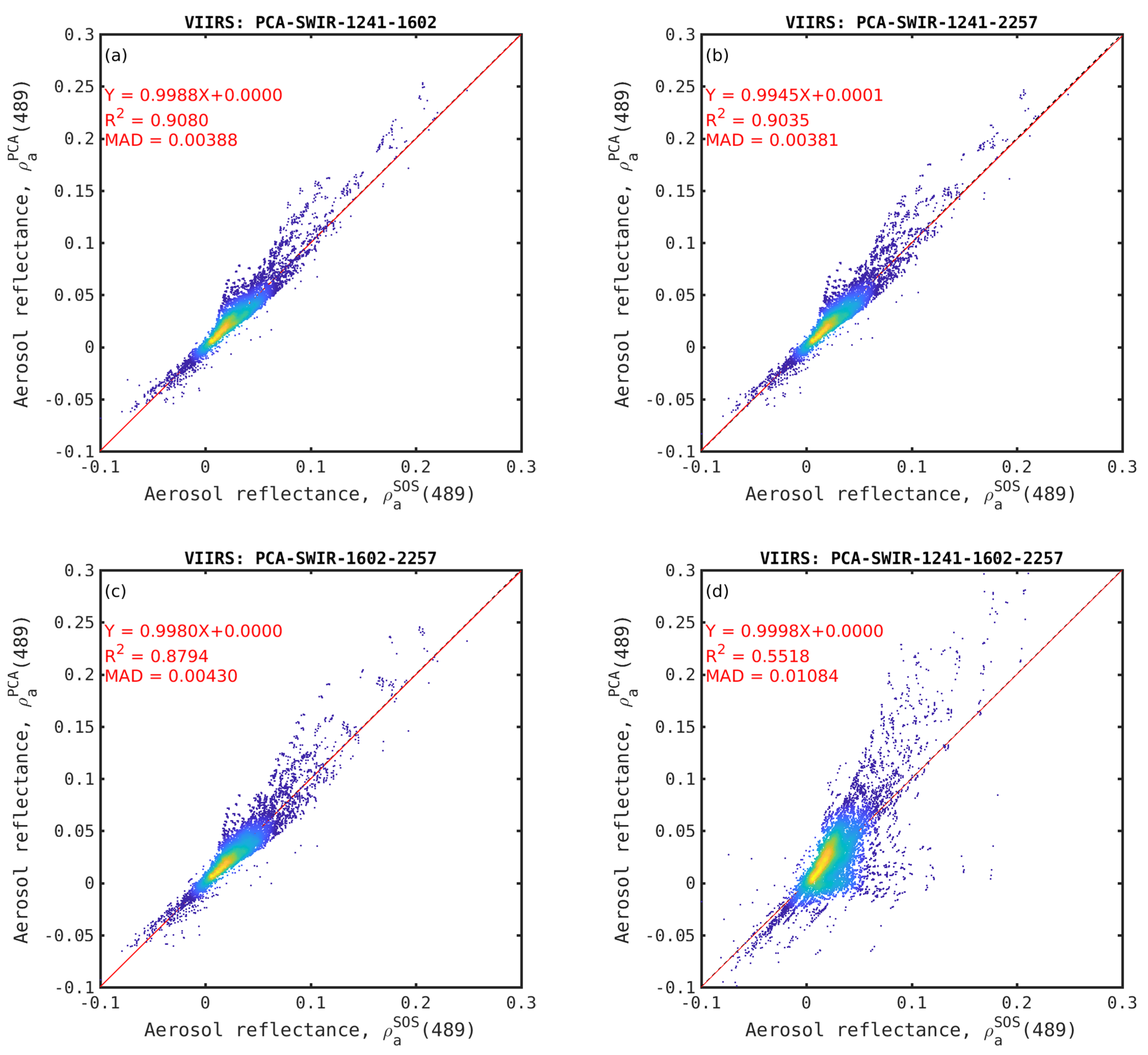
Remotesensing 13 01050 g005
Figure 6. Same as Figure 5 but for VIIRS 489 nm band using PCA-SWIR12 (a), PCA-SWIR13 (b), PCA-SWIR23 (c), PCA-SWIR123 (d) schemes.
Remotesensing 13 01050 g006
Figure 7. Same as Figure 6 but for 862 nm VIIRS band, (a), PCA-SWIR13 (b), PCA-SWIR23 (c), PCA-SWIR123 (d) schemes.
Remotesensing 13 01050 g007
Figure 8. Retrieved (ρwPCA) vs. field (ρwASD) water reflectance at SABIA-Mar (a) 765 nm (NIR1) and (b) 865 nm (NIR2) bands. Mean values are represented as red dots and vertical red bars correspond to the interquartile range (IQR).
Remotesensing 13 01050 g008
Figure 9. Retrieved (ρwPCA) vs. field (ρwASD) water reflectance at VIIRS 862 nm (NIR2) band using (a) PCA-SWIR12, (b) PCA-SWIR12, (c) PCA-SWIR12, and (d) PCA-SWIR12 schemes. Dots are mean values and bars are the interquartile range (IQR).
Remotesensing 13 01050 g009
Figure 10. Satellite-derived water reflectance ( ρ w sat ) vs. field water reflectance ( ρ w field ) in the BLUE band (~445 nm) for MODIS/Aqua (MA), MODIS/Terra (MT), VIIRS/NOAA20 (VNOAA20), and VIIRS/Suomi-NPP (VSNPP) sensors shown in red, green, blue, and magenta, respectively. Each inset corresponds to a different AC: (a) NIR iterative scheme (ITER-NIR), (b) Rayleigh correction AC, i.e., without aerosol correction (RC), (c) SeaDAS SWIR AC using bands SWIR1 and SWIR3 (GW94-SWIR13), and (d) PCA-SWIR13 AC (PCA-SWIR13).
Remotesensing 13 01050 g010
Figure 11. Same as Figure 10, but in the NIR2 band (~860 nm): (a) NIR iterative scheme (ITER-NIR), (b) Rayleigh correction AC, i.e., without aerosol correction (RC), (c) SeaDAS SWIR AC using bands SWIR1 and SWIR3 (GW94-SWIR13), and (d) PCA-SWIR13 AC (PCA-SWIR13).
Remotesensing 13 01050 g011
Figure 12. Satellite-derived vs. field reflectance (TriOS or ASD in black) using several AC schemes: ITER-NIR (blue), GW94-NIR (orange), GW94-SWIR13 (green), and PCA-SWIR13 (red) for different match-ups: (a) RdP_20130227_PP01-11 (VSNPP overpass), (b) RdP_20130430_PP02-03 (MT overpass), (c) RdP_20130430_PP02-12 (VSNPP), (d) RdP_20151118_St26 (VSNPP), (e) RdP_20160925_St12 (MT), and (f) RdP_20160925_St13 (MT). Solid dotted lines show mean values of the 3 × 3 pixel window and uncertainty areas are shaded. Missing values correspond to AC or match-up failures. Simultaneous field measured turbidity (obtained using a portable HACH 2100Qis turbidimeter) is indicated inside each panel.
Remotesensing 13 01050 g012
Figure 13. Comparison of spatial patterns of water and aerosol reflectance retrieved by PCA-SWIR13, GW94-SWIR13, GW94-NIR, and ITER-NIR ACs from MODIS/Aqua image of the Río de la Plata acquired on 2014-05-16T15:35:00Z. RGB composite (a), water (b,e,h,k), and aerosol (c,f,i,l) reflectance at 443 nm, retrieved using PCA-SWIR13 (b,c), GW94-SWIR13 (e,f), GW94-NIR (h,i), and ITER-NIR (k,l) schemes. Plots show aerosol vs. water reflectance in the Río de la Plata’s turbidity front region marked with squares (d,g,j).
Remotesensing 13 01050 g013
Figure 14. Same as Figure 13 but at 859 nm and not considering the performance of the GW94-NIR scheme, as it retrieves trivially null water reflectance in the NIR bands. RGB composite (a), water (b,e,h), and aerosol (c,f,i) reflectance at 748 nm, retrieved using PCA-SWIR13 (b,c), and GW94-SWIR13 (e,f), ITER-NIR (h,i). Plots show aerosol vs. water reflectance in the Río de la Plata’s turbidity front region marked with squares (d,g).
Remotesensing 13 01050 g014
Table 1. Spectral bands of the sensors used to theoretically test the SWIR-PCA algorithm. The bands in which the black water assumption is valid are marked in green. In yellow, the bands in which this assumption is affected only with very high sediment concentrations.
Band TagMODISVIIRSSABIA-Mar
BLUE443 nm443 nm443 nm
GREEN555 nm551 nm555 nm
RED645 nm667 nm665 nm
NIR1748 nm745 nm750 nm
NIR2859 nm862 nm865 nm
SWIR11240 nm1238 nm1240 nm
SWIR21640 nm1601 nm1640 nm
SWIR32130 nm2257 nm
Table 2. Atmospheric, surface, geometric, and optical parameters used as input to the sets of simulations using Centre National d’Études Spatiales/Successive Orders of Scattering (CNES-SOS).
CNES-SOS ParameterInput Value/Range
λ (Wavelength)400 nm to 2500 nm. step 2 nm (VIS/NIR) and 10 nm (far SWIR).
θs (Solar Zenith Angle, SZA)15° to 60° (step 15°)
θv (Viewing Zenith Angle, VZA)0° to 45° (step 15°)
ϕ (Relative Azimuth Angle, RAA)0° to 180° (step 15°)
ρw (Water reflectance)Set W: ASD in situ (RdP), see Figure 2
w (Wind speed)0, 2, 4, 8, 16 m/s
nw (Relative air–water interface)1.334
τr (Rayleigh optical thickness)Bodhaine et al., 1999 [22]
δr (Depolarization Factor)Bodhaine et al., 1999 [22]
Hr (e-folding height scale for molecules)8 km
τa (Aerosol optical thickness at 500 nm)0:0.1:0.4
dVa/dlnr (Aerosol granulometry)Continental, Marine, and Urban scenarios [23]
na + ima (Refractive index, aerosols)Continental, Marine, and Urban scenarios [23]
Ha (e-folding height scale for aerosols)2 km
nmax (Maximum scattering order)20
Ipol (Polarization index)1 (consider polarization)
Table 3. Specific inputs (aerosol correction type “aer_opt” and wavelengths of the corrector bands “aer_wave_short” and “aer_wave_long”) of each of the studied L2Gen atmospheric corrections (ACs). The band wavelengths used for aerosol calculations are here represented with the band tags of Table 1, since they depend on each sensor. General inputs to L2Gen that were not changed among ACs are mentioned in the text. GW94-NIR, NIR multi-scattering extrapolative approach; ITER-NIR, standard NASA’s iterative scheme in the NIR; GW94-SWIR, SWIR multi-scattering extrapolative approach; RC, Rayleigh correction.
Atmospheric Correction (AC)Aer_Opt (Description)Aer_Wave_ShortAer_Wave_Long
GW94-NIR−1 (Multi-scattering with 2-band model selection)NIR1NIR2
ITER-NIR−2 (Multi-scattering with 2-band, RH-based model selection and iterative NIR correction)NIR1NIR2
GW94-SWIR13−1 (Multi-scattering with 2-band model selection)SWIR1SWIR3
RC−99 (No aerosol correction)
Table 4. Cumulative variance explained with one, two, and three principal components of the simulated aerosol reflectance and inversion conditional numbers for the PCA-SWIR123 and PCA-SWIR13 schemes applied to VIIRS bands.
Band (nm) (Band Tag)PCA-SWIR123 (VIIRS) Explained Variance (%)Inversion Conditional NumberPCA-SWIR13 (VIIRS) Explained Variance (%)Inversion Conditional Number
1 Component2 Components3 Components (Total Used)1 Component2 Components (Total used)
443 (BLUE)69.0495.3699.43389.367.1495.424.8
551 (GREEN)73.5297.0499.5426.972.4697.284.0
667 (RED)77.0897.4999.6914.076.1697.703.4
74 (NIR1)79.4497.6999.7410.378.5097.922.9
862 (NIR2)82.8798.1099.816.281.9298.382.3
Table 5. (a). Eigenvector components of the PCA-SWIR13 AC scheme for MODIS/Aqua. Here, λtbc stands for the wavelength of the band to be corrected (i.e., either the BLUE, GREEN, RED, NIR1, or NIR2 band). (b). Same as Table 5a, but for VIIRS/Suomi-NPP.
Eigenvector ComponentBand to be Corrected
BLUEGREENREDNIR1NIR2
(a)
e1PCAtbc)0.567540.641030.647830.637710.62218
e1PCA(SWIR1)0.620190.579740.572760.57660.58281
e1PCA(SWIR3)0.541530.502970.502260.510740.52271
e2PCAtbc)0.800750.730230.708760.696810.66258
e2PCA(SWIR1)−0.26275−0.25892−0.2115−0.14924−0.03639
e2PCA(SWIR3)−0.53829−0.63223−0.673−0.70155−0.74811
e3PCAtbc)−0.19155−0.2363−0.27924−0.32829−0.41698
e3PCA(SWIR1)0.739140.772570.791970.803280.81179
e3PCA(SWIR3)−0.64574−0.58932−0.54297−0.49696−0.4088
(b)
e1PCAtbc)0.570840.641130.648760.63920.62309
e1PCA(SWIR1)0.622110.583090.575210.578710.58499
e1PCA(SWIR3)0.535830.498950.498240.506480.51918
e2PCAtbc)0.794390.725370.70050.687220.64802
e2PCA(SWIR1)−0.25348−0.24815−0.19558−0.13422−0.01441
e2PCA(SWIR3)−0.55199−0.64208−0.68633−0.71394−0.76149
e3PCAtbc)−0.20758−0.25057−0.29734−0.34518−0.43798
e3PCA(SWIR1)0.740760.773580.794280.804420.81091
e3PCA(SWIR3)−0.6389−0.58205−0.52981−0.48349−0.38806
Table 6. Noise-equivalent RC reflectance for each of the MODIS/Aqua sensor bands in the NIR and SWIR, obtained by applying the geostatistical method to the RC reflectance of the mentioned set.
Wavelength (nm) (Band Tag)Noise Equivalent Reflectance, NEρRC
748 (NIR1)0.001845
859 (NIR2)0.003686
1240 (SWIR1)0.000279
1640 (SWIR2)0.000178
2130 (SWIR3)0.000174
Table 7. Comparison between performance metrics of simulated water reflectance ρw (PCA) vs. ρw (field) at MODIS/Aqua 857 nm band (Set W) with and without noise added to simulations. MAD, mean absolute difference; Int, intercept.
AC/SensorNoise AddedMADSlopeIntR2
PCA-SWIR13 MODIS/AquaNo0.00050.984−0.00060.999
Yes0.00081.006−0.00080.998
Table 8. Performance metrics of satellite-derived water reflectance (ρwsat) vs. field water reflectance ( ρ w field ) in the BLUE, GREEN, RED, NIR1, and NIR2 bands of MODIS/Aqua (MA), MODIS/Terra (MT), VIIRS/NOAA20 (VNOAA20), and VIIRS/Suomi-NPP (VSNPP) sensors. Results are shown for ITER-NIR, GW94-NIR, GW94-SWIR13, and PCA_SWIR13 ACs. RMSE, root mean square error; MAD, mean absolute difference; MAPD, mean absolute percentage difference; MD, mean difference.
BandACN#NegRMSEMADMAPDMDSlopeIntR2
BLUEITER-NIR950.0370.03293.7−0.0260.0740.0000.000
GW94-NIR660.0390.035104.2−0.0511.011−0.0540.663
GW94-SWIR132050.0310.02570.0−0.016−0.1540.0360.170
PCA-SWIR133410.0270.02474.30.0190.3300.0410.061
GREENITER-NIR1600.0350.02734.6−0.0080.2140.0390.233
GW94-NIR1750.0430.03649.5−0.049−0.1410.0240.072
GW94-SWIR133600.0250.01722.2−0.0060.4260.0370.297
PCA-SWIR134000.0200.01723.90.0110.5360.0460.429
REDITER-NIR2770.0530.04040.8−0.0330.1470.0550.047
GW94-NIR3410.0480.03432.9−0.0330.5030.0140.161
GW94-SWIR134000.0190.01514.7−0.0020.6790.0260.656
PCA-SWIR134000.0230.01920.50.0130.8120.0270.671
NIR1ITER-NIR1700.0170.01326.9−0.0080.4900.0140.847
GW94-SWIR133400.0110.00716.4−0.0040.9350.0020.843
PCA-SWIR133700.0090.00716.00.0001.0290.0020.866
NIR2ITER-NIR2140.0220.01550.5−0.0140.1980.0120.113
GW94-SWIR133200.0160.00932.2−0.0030.9080.0010.882
PCA-SWIR133300.0150.00827.50.0000.9960.0000.920
Publisher’s Note: MDPI stays neutral with regard to jurisdictional claims in published maps and institutional affiliations.

