Two Independent Light Dilution Corrections for the SO₂ Camera Retrieve Comparable Emission Rates at Masaya Volcano, Nicaragua

Abstract

SO₂ cameras are able to measure rapid changes in volcanic emission rate but require accurate calibrations and corrections to convert optical depth images into slant column densities. We conducted a test at Masaya volcano of two SO₂ camera calibration approaches, calibration cells and co-located spectrometer, and corrected both calibrations for light dilution, a process caused by light scattering between the plume and camera. We demonstrate an advancement on the image-based correction that allows the retrieval of the scattering efficiency across a 2D area of an SO₂ camera image. When appropriately corrected for the dilution, we show that our two calibration approaches produce final calculated emission rates that agree with simultaneously measured traverse flux data and each other but highlight that the observed distribution of gas within the image is different. We demonstrate that traverses and SO₂ camera techniques, when used together, generate better plume speed estimates for traverses and improved knowledge of wind direction for the camera, producing more reliable emission rates. We suggest combining traverses and the SO₂ camera should be adopted where possible.

1. Introduction

Gas emissions from volcanoes are a key indicator of volcanic activity, as their release closely links to magma ascent dynamics [1,2,3]. The most common gas species in hot plumes are, in typical order of abundance, H₂O, CO₂ and SO_2, followed by halogen species [4,5]. Volcanologists commonly measure sulfur dioxide emission rate due to its high plume and low atmospheric concentration, as well as pronounced UV absorption [6]. It can be used as a proxy for total gas emissions through combination with in-plume gas ratio measurements made by instruments such as FTIR, Multi-GAS or alkali filter packs [7,8,9,10]. Trends in gas emission can be combined with other volcanological signals, such as seismic and surface deformation, to gain a more complete understanding of activity [11,12,13,14].

To obtain a single SO₂ emission rate, scientists must measure an SO₂ cross-section of the volcanic plume and estimate the plume speed. A cross-section can be obtained in a number of ways. Typically, a spectrometer measures a series of slant column densities (SCDs) through the plume, which combine to yield the cross-section. For short-term campaigns, traverses underneath the plume use a vertically pointing telescope moved by road vehicle, on foot or in the air by UAV or helicopter [15,16,17,18]. Longer deployments must use less personnel intensive techniques, such as permanent scanner networks (e.g., the NOVAC and FLAME networks) [18,19] or vertically pointing spectrometer arrays [20].

The SO₂ camera is another SO₂ emission rate measurement technique [21,22,23,24]. Rather than create a single cross-section over minutes, it instead captures many cross-sections through the plume with a single image. Its use has mostly been restricted to short campaigns [25,26,27], though has seen a growing number of longer deployments on Etna, Stromboli and Kīlauea [28,29,30,31]. It measures SO₂ emission rate with a high spatial [32] and temporal resolution [33]. The temporal resolution is significantly greater than standard monitoring capabilities, which are limited by the ~5 min scan duration [18] or the tens of minutes needed for a traverse (depending on plume size and terrain). This greater temporal resolution is well suited for imaging many rapid degassing processes occurring at volcanoes, such as puffs and Strombolian explosions [25,34]. Furthermore, the SO₂ camera is still useful at some volcanoes with less variable gas emissions, as plumes can become uneven through buoyant rising in turbulent ground-level wind fields [35].

Scattering of light in the atmosphere is a known issue that causes large errors in UV spectroscopic quantification of SO₂ emission rate. It can be particularly important for SO₂ cameras, as to get an optimum view they may be positioned several kilometers away from the plume. There are two different scattering regimes [36,37]. One is Mie scattering, which occurs when photons scatter off aerosol particles much larger than the wavelength of the light. On a clear day, with few clouds, the air between the plume and camera will be largely free of such aerosols, except where the hot volcanic plume begins to cool and condense. Under these optimal conditions, Mie scattering effects are small, so measurements several kilometers from the plume can instead consider Rayleigh scattering as dominant. Rayleigh scattering occurs due to light interacting with small gas molecules in the atmosphere. As the distance from the volcano increases, light that has not travelled through the plume increasingly replaces the light that has travelled through the plume. This leads to “light dilution” of the plume signal. The effect can easily cause a >50% underestimate in the SO₂ emission rate at a measurement range of a few kilometers [37,38,39], though long-term SO₂ flux trends from permanent deployments often show good agreement with other independent monitoring techniques [14].

One key decision for SO₂ camera operators is the calibration method. Unlike a spectrometer, SO₂ camera imagery does not directly retrieve SO₂ SCD. Instead, it retrieves optical depth, which is roughly proportional to SCD, but the constant of proportionality can change with different illumination conditions. The original calibration method places small gas containers containing known SO₂ SCDs, known as cells, in the path of the instrument, then records the optical depth response [21]. A later alternative suggests calibrating a small region of the camera using a co-located spectrometer pointing into the field of view of the camera [33]. Studies examining calibration differences between using spectrometers and cells suggest cell calibration can fail to account for the full effect of aerosols, artificially inflating the calibration by up to 20% [40].

Previous studies do not compare the two calibration methods, cell and spectrometer, when properly correcting for radiative transfer effects [40]. In this paper, we analyze three days of SO₂ camera imagery from Masaya volcano, Nicaragua, captured in January 2018. We show that an adapted version of the volcanic edifice image-based correction [41,42] and calibration using dual-waveband spectra correction [38,43] retrieve comparable SO₂ emission rates for the imagery but give different gas distributions in the plume. We highlight weaknesses in both methods, then suggest a combination of image-based and spectrometer corrections should be used for ideal measurements. We confirm our measured emission rates with simultaneous traverses, highlighting the increased reliability in measurements obtained from combining the strengths of each of these techniques.

2. Materials and Methods

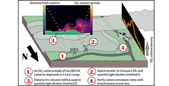
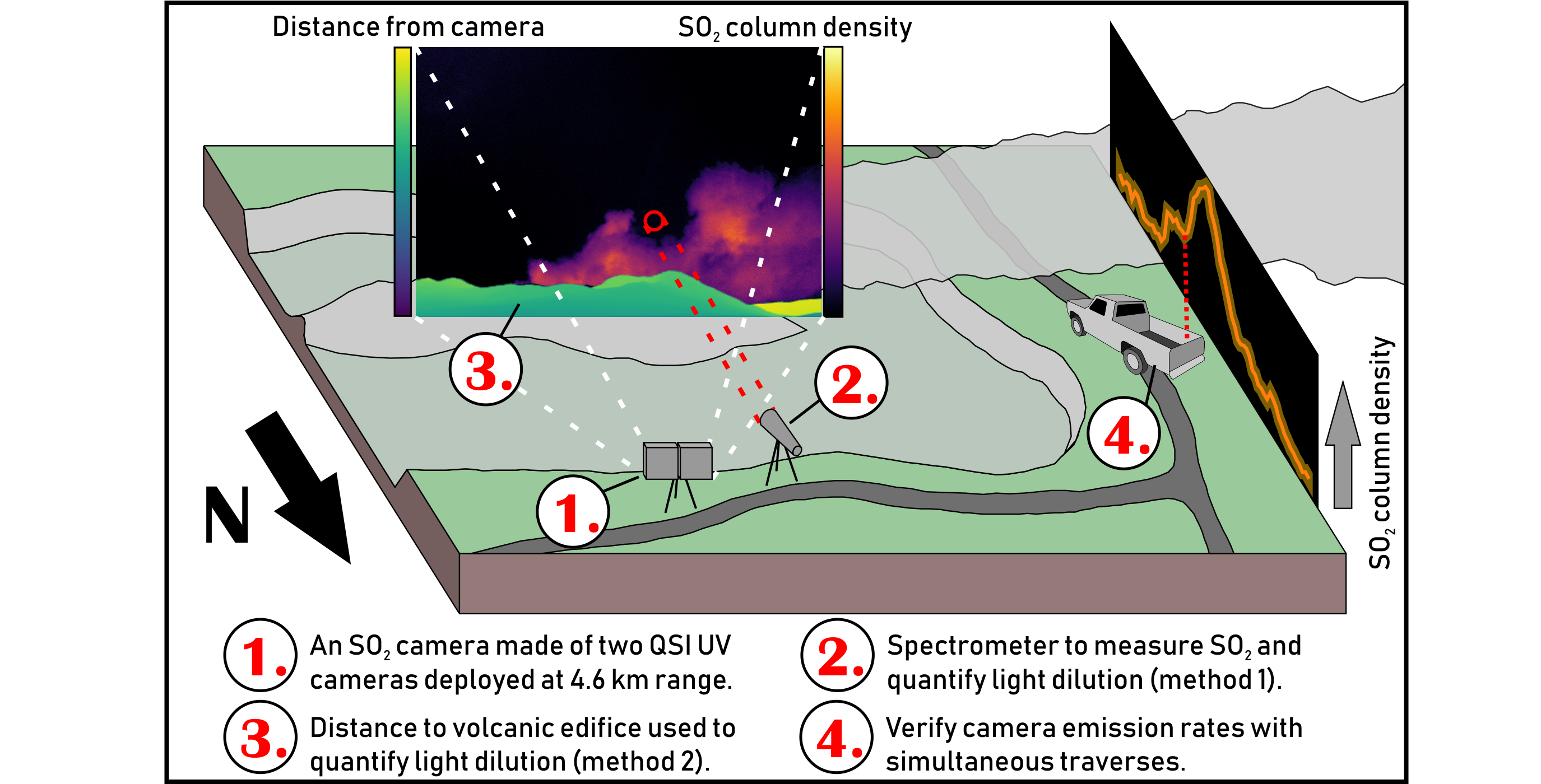
Our setup at Masaya volcano is described in Section 2.1, then a brief summary of the basic SO₂ camera principles is provided in Section 2.2. We describe three different methodologies that correct for light dilution and two that calibrate SO₂ camera-measured optical depths into SO₂ SCD images. First, we calibrate an SO₂ camera with a co-located spectrometer, correcting for dilution using dual-waveband modelling (Section 2.3 and Section 2.4). Second, we calibrate using SO₂ gas cells and correct for dilution using scattering efficiencies derived from reflected light from the volcanic edifice (Section 2.5). We also suggest a combined approach using the dilution-corrected co-located spectra and image-based dilution from the volcanic edifice. Third, we reuse these scattering efficiencies to create an extinction correction that assumes the falloff in SO₂ measured in roughly exponential with distance, again calibrating with SO₂ cells (Section 2.6). We outline the correlation method for plume-speed determination (Section 2.7). We then highlight methodological improvements that we can utilize because we simultaneously measure the plume by SO₂ camera and traverse (Section 2.8).

2.1. Setup

Our SO₂ camera consisted of two QSI RS2.0 UV cameras mounted in a metal frame. Each camera had an Edmunds Optics bandpass filter with a full-width half-maximum of approximately 10 nm, with the on-band filter centered at 310 nm and the off-band filter at 330 nm. The filter was mounted in front of the quartz lens (Universe Optics) due to equipment constraints, though this is suboptimal [33]. We fixed the exposure time for both cameras, with the 310 nm camera set to 0.4 s and the 330 nm camera set to 0.1 s.

We deployed our SO₂ camera on Masaya volcano on the 10th, 13th and 15th January 2018, capturing images at a framerate of 0.2 Hz. Conditions were generally favorable. Within the camera field of view there were generally few clouds, though on occasion they passed between the sun and terrain, changing the illumination. The camera was situated at the Mirador viewpoint (12.0245° N, 86.1795° W), some 4.6 km away from the vent. On the 15th January, we set up a collimated telescope with an attached Hoya U330 visible-cut filter to reduce stray light. It connected via fiber optic cable to an Ocean Insight (formerly Ocean Optics) FLAME-S-UV-VIS spectrometer, which was available from 10:47 to 11:54 local time (UTC-6). This spectrometer has a wavelength range from 255 to 405 nm. It recorded composite spectra made from 10 co-added spectra, each with a 500 ms integration time.

We also affixed an additional collimated telescope to a car to conduct traverses beneath the plume on all three days, aiming for them to coincide with the camera measurements. On the 13th, the FLAME spectrometer outlined above was used for the traverses with the same integration time and co-adding settings, but on the 10th and 15th, a different Ocean Insight FLAME-S-UV-VIS spectrometer was used instead. This spectrometer has a wavelength range from 298 to 436 nm and was set to an integration time of 400 ms on the 10th and 500 ms on the 15th, with 10 co-adds. The attached telescope was not visible-cut filtered on these days, so the spectra may be affected by stray light, though a correction for this is applied in the analysis. In all traverses, we drove along the Ticuantepe road, typically intersecting the plume some 5 km south-west of the volcanic vent. An overview of the measurement locations is given in Figure 1.

2.2. Camera Analysis in Brief

A single SO₂ camera is usually made from two individual UV cameras capturing images simultaneously, each with a different bandpass filter attached [21], though some versions use a single UV camera [22,25]. One bandpass filter is centered around 310–313 nm, which detects SO₂ absorption, whilst the second is centered at 330 nm, correcting for any flat light reduction that occurs in the same wavelength region due to influences such as clouds and aerosol.

Three image pairs are needed to make a single SO₂ camera image. Firstly, each of the two cameras simultaneously captures an image of the plume. A dark image for each camera, captured with a closed mechanical shutter, then corrects for the CCD having a non-zero response to zero light input. Also required are clear images, which show the intensity of light that arrives at the camera from each direction if the plume were not present. In practice, clear images are obtained by panning the camera to an area of plume-free sky as near to the plume as practicable. We captured clear images in small breaks in camera measurements, and at least once per hour. This means we have two sets of clear images on both the 10th and 13th, and four sets for the 15th.

The processing of the images can be summarized in the equation below, which yields an optical depth for each pixel:

$$O{D}_{\left(i,j\right)}=-\ln \left[\frac{\left(P{A}_{\left(i,j\right)}-D{A}_{\left(i,j\right)}\right)/\left(C{A}_{\left(i,j\right)}-D{A}_{\left(i,j\right)}\right)}{\left(P{B}_{\left(i,j\right)}-D{B}_{\left(i,j\right)}\right)/\left(C{B}_{\left(i,j\right)}-D{B}_{\left(i,j\right)}\right)}\right]$$

(1)

where $O{D}_{\left(i,j\right)}$ is the optical depth at the i-th row and j-th column of camera CCD pixels. Inside the logarithm, “A” and “B” represent the camera with the 310 and 330 nm filters, respectively. The first letters, “P”, “D” and “C” represent plume, dark and clear images.

Images of plume-free sky can only approximate the light intensity behind the plume. This leads to a residual in the optical depth images, which should be corrected [42]. The residual is spatially continuous, so studies should remove this residual with linear offsets or polynomials determined using areas of the camera image known not to contain SO₂. We first correct variations in the residual through time by subtracting the average optical depth of a plume- and cloud-free 100 × 100 pixel area in the top left of each image. We then correct the spatial distribution in the residual along only the integration lines used to calculate SO₂ emission rate (see Section 2.7). Polynomial fits were poorly constrained because there is no plume-free sky underneath the plume, and they often created substantial unphysical negative optical depths at the bottom of the plume close to the skyline. Instead, we use a 101 sample, 3rd order polynomial Savitzky–Golay filter on the integration line in each measurement period with the most plume-free pixels, using the last plume-free pixel optical depth residual, as determined by the filter, across the remaining section of plume. This gives the remaining optical depth residual along the integration line, which is then subtracted. This approach appears to be an effective compromise, accurately removing the known plume-free residual whilst avoidingnegative optical depths within the plume.

An SO₂ camera requires calibration to convert measured optical depths into SCDs. The calibration can change over time, varying by up to 20% over about 2.5 h either side of midday [44]. The calibration also varies with the angle at which light passes through the bandpass filters attached to the camera, creating a variation of up to 25% [33,40]. There are two common approaches to calibration, and each approach requires its own tailored light dilution correction method (Section 2.4 and Section 2.5).

The first approach is to correlate the optical depth values with SO₂ SCDs measured by a collimated co-located spectrometer. If the spectroscopy is accurate, this produces a reliable calibration within the field of view of the spectrometer [33], though it requires multiple SO₂ SCDs from the spectrometer and optical depths from the camera to produce a single calibration value [28]. The exact viewing spot for the spectrometer can be determined experimentally in the lab, but since our setup could move in transit, we chose to correlate the spectrometer time series with our image optical depth time series. We first find the pixel with the best correlation to the spectrometer SO₂ SCD time series, then independently vary the size of the spectrometer field of view [42]. We correlate using a simple average of the optical depth of all pixels within the field of view. This is an approximation and would be inaccurate if there is a large heterogeneity within the field of view [45]. However, our spectrometer field of view is small, at less than 1°, so there should not be much heterogeneity present.

A second calibration method uses a series of gas containers with known SO₂ column densities placed in turn into the camera’s field of view to define a calibration [21]. Ideally, these cells cover the entire field of view of the camera to allow correction of the angle dependency of the filters [33,40]. Our cells were too small for this, so we obtained a single optical depth for the entire field of view for each cell. This produces a single calibration value. We only obtained a single calibration value across all three days, performed between 21:05 and 21:09 UTC on 10th January, using five cells, with values of 93, 195, 482, 993 and 1802 ppm.m. The manufacture’s quoted error in the cell SO₂ column density is ± 10%.

2.3. Spectroscopy

Differential optical absorption spectroscopy (DOAS) is widely used to retrieve SO₂ SCD from a single spectrum, with many available implementations including QDOAS and DOASIS [46,47]. In this paper, we use an intensity fitting software called iFit [48] to analyze our spectra both from traverses and from the spectrometer co-located with the camera. The code is available online [49]. We fit for SO₂ at 295 K [50], O₃ at 233 K [51], Ring pseudo-absorber [52] and a background polynomial for broadband changes in intensity. To correct for pixel-to-pixel variation introduced in the manufacturing process, we include a pre-measured flat spectrum for the specific spectrometer. We also use fixed instrument line shape parameters for each measurement period, determined from SO₂-free spectra. We include a baseline offset in the fit for spectra captured without a visible-light filter correcting for stray light. We use two different overlapping wavelength windows for the spectroscopy [21,43], specifically 306–316 nm and 312–322 nm, to facilitate light dilution correction (Section 2.4).

2.4. Light Dilution and Correcting Spectra Analysis

Light dilution occurs when photons that travelled through the plume are scattered out of the instrument field of view, and when photons that did not travel through the plume are scattered into the instrument field of view. Assuming only a single scatter is occurring, we can make the following expression to describe the intensity of light, $I\left(\lambda \right)$, that arrives at the instrument at each wavelength [41,53]:

$$I\left(\lambda \right)=I_p\left(\lambda \right)·\exp \left(-\sigma \left(\lambda \right)·d\right)+I_A\left(\lambda \right)·\left(1-\exp \left(-\sigma \left(\lambda \right)·d\right)\right)$$

(2)

where $I_p$ is the original intensity of the light after passing through the plume but before dilution, $I_A$ is the intensity of the background sky and d is the distance between the plume and instrument. $\sigma \left(\lambda \right)$ is the scattering efficiency of the atmosphere, which will depend on atmospheric conditions, such as air pressure, temperature and composition [54]. It is proportional to λ⁻⁴ when Rayleigh scattering off small molecules dominates but is proportional to approximately λ^−1.3 when Mie scattering off larger aerosols dominates.

Some simplified corrections assume that the falloff in SO₂ column density with distance follows the falloff in intensity of light that has passed through the plume [55]. This correction with an extinction coefficient uses the following approximation:

$$S\approx S_O·\exp ·\left(-\sigma \left(\lambda \right)·d\right)$$

(3)

where $S$ is the measured SO₂ SCD, and $S_O$ is the actual SO₂ SCD present. The equation requires a scattering efficiency, which can be estimated by comparing the SCD measured at two different distances from the plume. Sometimes, it is instead estimated from measurements conducted at other volcanoes under similar conditions [40]. If used incorrectly, it is expected to cause an underestimation of SO₂ SCD, especially in the densest parts of the plume. Despite an acknowledgment that the approximation is incorrect at high SO₂ column densities, it has seen some use in correcting SO₂ camera SCDs [40,56].

Some studies use a more detailed correction to avoid the underestimation problem. Monte-Carlo simulations estimate the paths of all photons that contribute to the final intensity [37,57], allowing a very accurate correction where parameters such as plume conditions and geometry are known. Later work added the creation of lookup tables, facilitating automatic iteration of these parameters to fit the observed spectra [39], though the base simulations are still complex and are not in widespread use for ground-based volcanology [58].

In this paper, we correct our spectra using a third method, which uses the SO₂ SCD measured by a spectrometer at two different wavelength windows [38,43]. This avoids the need for Monte-Carlo simulations. It uses an altered version of iFit [48] to model and re-analyze spectra, creating a lookup table to correct the SO₂ SCD. Light dilution causes a greater underestimation in SO₂ SCD retrieved at lower wavelengths, where the SO₂ absorption is larger and UV scattering more efficient, allowing quantification of the dilution and hence correction. The method requires a number of additional assumptions, including that dilution dominates over other scattering effects in a largely aerosol-free sky.

The first of our SO₂ camera light dilution methods mentioned at the start of Section 2 uses this spectra correction. We correlate corrected SO₂ SCDs measured by the co-located spectrometer with raw optical depths measured by the SO₂ camera, producing a corrected calibration. This method has a weakness in using raw camera optical depths, as these depend on light dilution as well as SO₂ SCD. Therefore, large changes in light dilution during a measurement period will lead to an inaccuracy in the calibration. We use a single calibration for each measurement period but allow it to change after each acquisition of clear images.

2.5. Correct Optical Depth Images for Dilution

Rather than use a spectrometer to correct the camera for light dilution, it is possible to use only information available in an SO₂ camera image, directly correcting the image optical depth. These optical depths then convert into SCDs using the cell calibration described in Section 2.2. This can only be achieved if the scattering efficiency of the atmosphere is known in the wavelength range of each camera filter.

The first effort to correct light dilution in SO₂ camera measurements used multiple SO₂ camera locations to track the falloff in image contrast with distance [22], which could then be used to estimate the scattering efficiency. It makes use of an equation that is a simple rearrangement of Equation (2):

$$C_d=C_0·\exp \left(-\sigma \left(\lambda \right)·d\right)$$

(4)

where $C_d$ is the plume contrast at distance d, and $C_0$ is the actual plume contrast if no dilution was present. The plume contrast can be expressed as below:

$$C=\left(I_p-I_A\right)/I_A$$

(5)

where $I_p$ is the intensity of light from the plume measured on one camera, and $I_A$ is the intensity of light received by the camera if no plume was present.

These equations, however, first require an estimate of the scattering efficiency. This estimate can be obtained by simultaneously measuring the contrast of plume at two different distances. However, often, only a single SO₂ camera is available, so for such studies, the camera is deployed first at one distance then the next. As the measurements of the plume are not simultaneous, conditions likely change between the deployments, such as sunlight intensity, degassing strength or atmospheric visibility, which would introduce substantial uncertainties into this method.

Rather than measuring the plume from multiple distances, a single SO₂ camera can instead directly retrieve the scattering efficiency by examining how the intensity of light coming from the landscape changes with distance from the camera [41]. Most SO₂ camera images contain some volcanic edifice, which appears “washed out” in images taken at a distance of several kilometers from the volcano. Light reflected from more distant edifice has a greater path length for scattering to occur in, so shows more evidence of dilution. Currently, this image-based correction relies on lines of pixels in the volcanic edifice that have a constant slope and reflectivity. If such a line is identified, then the distance and intensity of a set of pixels can be substituted into Equation (2), but swapping the intensity of the edifice for the intensity of the plume. The process is repeated individually for each SO₂ camera image frame.

In the foreground of our images, however, we have a large area of ground covered in patchy vegetation, which can reflect light unevenly depending on the plant coverage. This is not ideal for the original image-based correction, as it restricts the area of the edifice we could use for the correction. As a result, it is challenging to calculate the distance to a set of pixels in the image. Instead, we use topography maps to calculate the distance to the part of the edifice in each pixel, though care must be taken to ensure the maps are of sufficient resolution. The available version of this method that we are aware of, however, requires knowledge of the exact location and viewing direction (i.e., pitch, roll and yaw) of each pixel in the camera [42], and this technique has been demonstrated for a single line of camera pixels only.

To overcome these issues, we expand and further develop the technique to create a full virtual 3D terrain using the NASA 1 arc second resolution (~30 m) Shuttle Radar Topography Mission (SRTM) data [59]. We project the topography onto the camera image plane, giving pixel coordinates for each topographic point to create a virtual image of the edifice, which is then compared to the measurement images. We manually iterate the viewing parameters of the camera to within ~1° of the correct viewing configuration, then run an automatic iteration of the viewing parameters using SciPy’s COBYLA minimization [60] to best match our virtual topography to the terrain in the image. Our code for this section is available online at https://github.com/matt-varnam/CalypSO. We then mask out both vegetated areas and areas in the plume shadow, using the remaining edifice to fit Equation (2) and retrieve the scattering efficiency independently for the on- and off-band cameras. Conceivably, at other volcanoes, the mask could be used to block areas of high reflectivity, such as a snow-capped peak.

The method has significant advantages compared to the DOAS calibration, as it does not require a spectrometer to be simultaneously pointing into the field of view. The correction can also be performed for each image pair, allowing a more dynamically varying correction through time. However, spectroscopy light dilution corrections are more widely applicable, as strong aerosol absorptions are thought to cause larger errors for the SO₂ camera, even when a second bandpass filter is used to correct for some of the aerosol effects [40].

As an additional methodology, we calibrate image-based corrected optical depth imagery, as outlined in this section, with dual-waveband corrected SO₂ SCDs measured by the collocated spectrometer. This combined approach should be the most robust, combining advantages from each.

2.6. Extinction Light Dilution Correction

As a comparison to our other light dilution corrections, we apply the extinction correction outlined in Equation (3) (Section 2.4) to our uncorrected cell-calibrated SCDs. We reuse the scattering efficiency measured by our 310 nm UV camera (Section 2.5) for this correction. This method is expected to cause an underestimation of SO₂ SCD, especially in the thickest parts of the plume, but we use it to determine the validity of the approximation in Equation (3) when applied to SO₂ camera measurements.

2.7. Plume Speed

The plume cross-section measured by the camera can be converted into an emission rate by multiplying by the apparent plume speed along an integration line. The simplest method is through cross-correlating two cross-sections at different locations in the image [21], but particle or flow tracking algorithms can more accurately determine the complex motion of a plume [28,44,61]. We use the simple correlation method as the plume is grounded in many of our images, making tracking the plume velocity more difficult [62]. The simple correlation assumes that the plume velocity is constant across the entire image and throughout a single measurement period. However, here, we simply want to compare the corrections, so assuming a uniform flow field also avoids the generation of additional differences between the calibration methods that are solely due to different wind profiles.

2.8. Complementarity of SO₂ Camera and Traverses

It is difficult to retrieve the wind direction directly from the SO₂ camera, though it is necessary to calculate the emission rate. Wind direction determines the distance to the plume in each camera pixel, required to convert SCD images into SO₂ cross-sections. Additionally, the increase in cross-section measured when the plume is not moving perpendicular to the camera viewing direction does not entirely cancel with the reduced plume speed observed [63]. This fact can be used to measure and correct for the wind direction. The discrepancy between SO₂ cross-sections as the plume travels across the camera field of view can be used to estimate wind direction, improving distance and, therefore, flux estimates.

However, traverses supply a reliable and more readily available measurement of the wind direction, provided the plume has travelled in approximately a straight line between the vent and traverse road. Wind directions for our traverses within each day are similar (±7°), so we use the average location of the plume center of mass across all traverses on a single day to estimate the wind direction for that day. This allows a more accurate estimate of the distance to the plume in each camera pixel, as well as correction for the up to 25° oblique angle of the measurements.

Measurements with the SO₂ camera can be used to improve the accuracy of traverse measurements. Traverses do not measure wind speed, so often use weather models or ground-based anemometers, both of which will often be inaccurate estimates of the actual plume speed [6]. Using the wind direction determined above and the apparent plume speed observed by the camera, we use geometry to calculate the actual plume speed. We then use this plume speed to convert our SO₂ traverse cross-sections into SO₂ emission rates.

Previous work has shown comparable emission rates through time between an SO₂ camera and scanners [29,56], though attempts to match camera measurements to traverses have not compared the short term temporal changes in the two methods [64].

3. Results

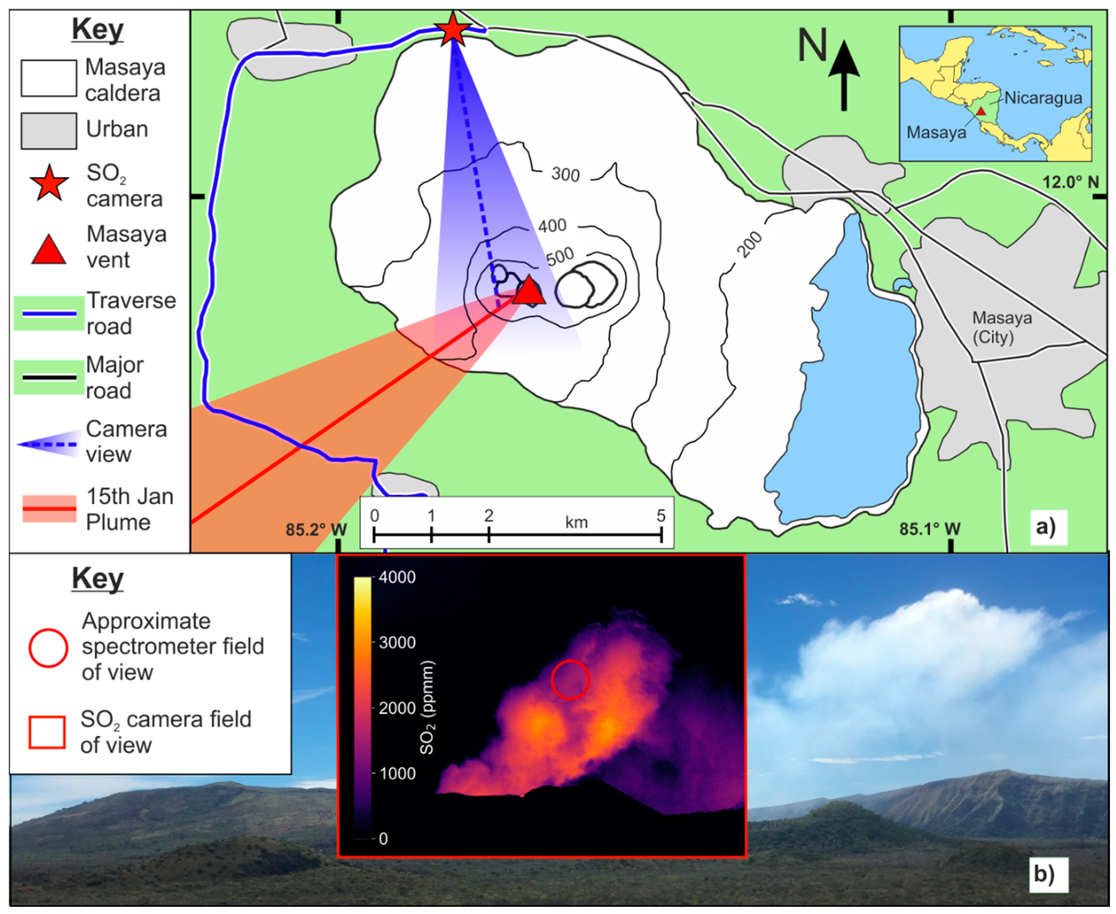
3.1. Estimates of Scattering Efficiency from the Improved Image-Based Technique

The synthetic skyline made using projected space-measured radar topography data closely matches the outline of the edifice in the real SO₂ camera imagery, confirming that the techniques used to transform the topography into the camera image plane have provided a true match for the camera images. In the projected topography, a distinct break in slope is visible at around 3.5 km away from the camera at the base of the closest cone (Figure 2a). The flat area in front of the cone is angled shallowly compared to the viewing direction of the camera, so would likely be subject to more error even if it were not vegetated. Beyond a distance of 4.0 km, the plume shadow affects the illumination of the edifice. We, therefore, retrieve the scattering efficiency (Figure 2b) using all pixels that lie between 3.5 and 4.0 km away from the camera, obtaining a good fit (Figure 2c,d).

This fit yields a moderately variable scattering efficiency between 0.070 and 0.150 km⁻¹ across all three days. In some data periods, there are abrupt jumps of up to 0.05 km⁻¹. The most abrupt changes measured in scattering efficiency are also seen in the intensities measured in the raw camera imagery. The probable explanation is that when passing clouds obscure the sun from the plume and edifice, the scattering efficiency will change due to the decrease in direct sunlight diluting the measurement.

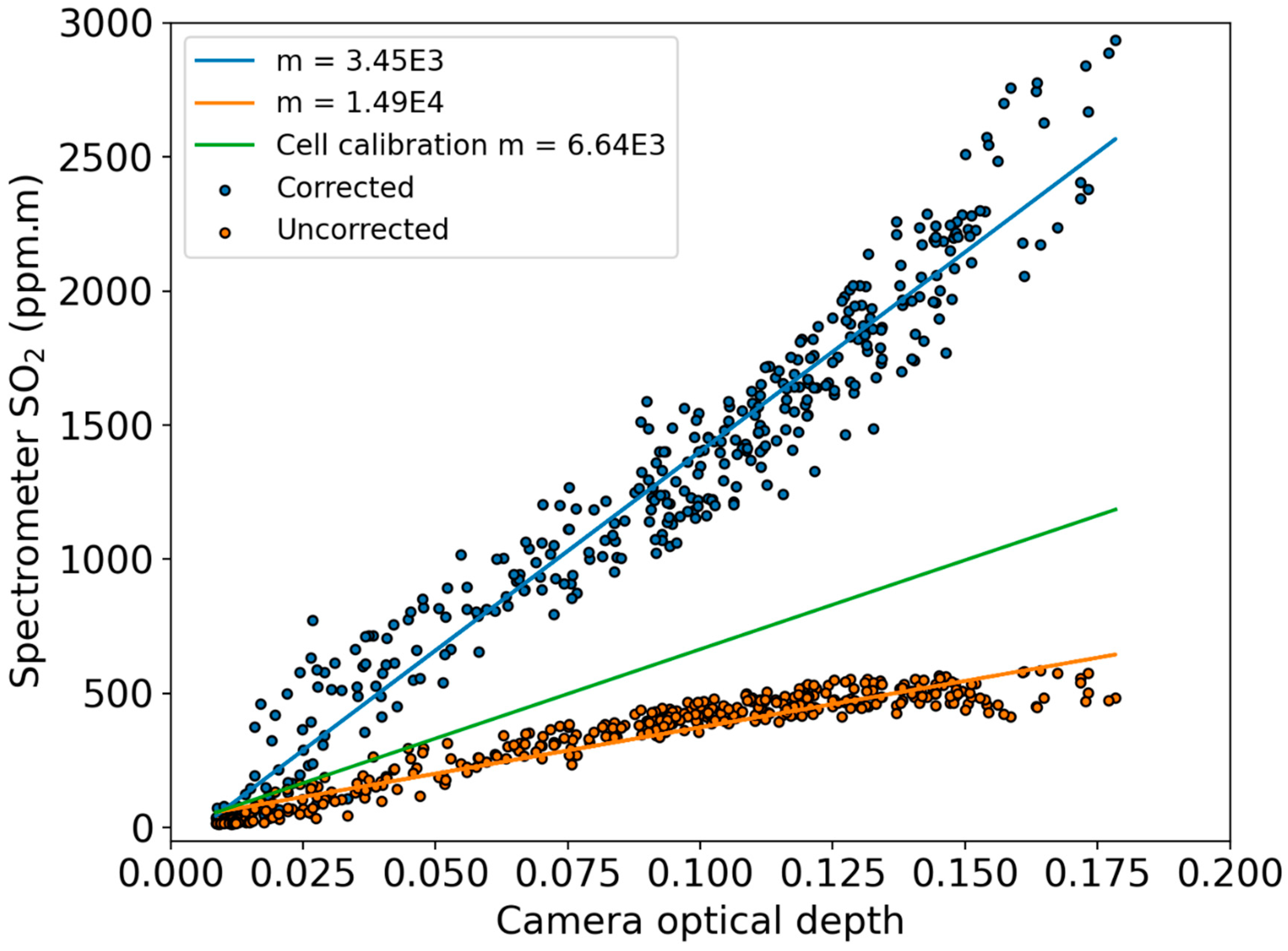
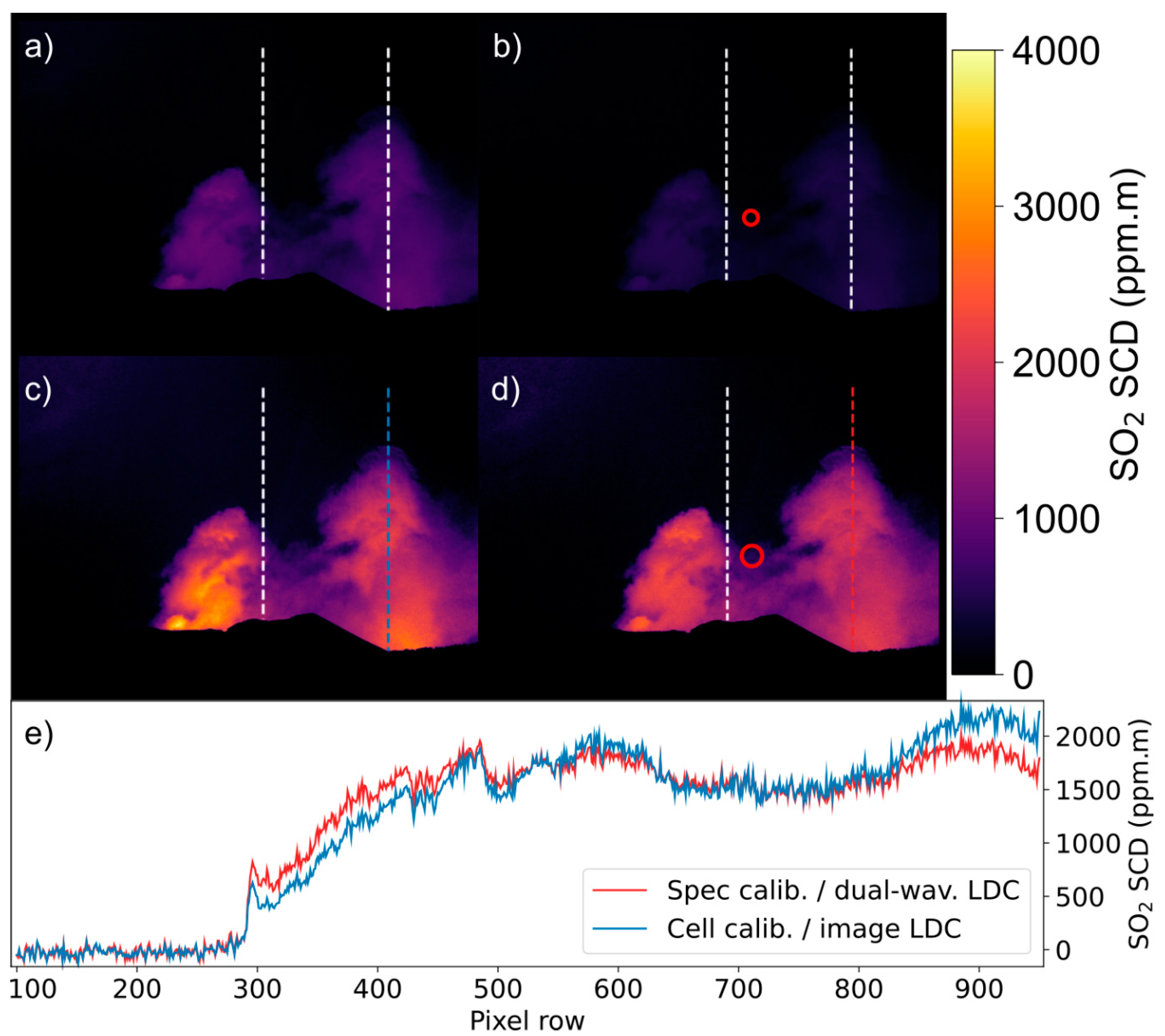
3.2. SO₂ Calibration and Column Density Images

Using our SO₂ cells of a known SCD, we get a calibration coefficient of 6640 ppm.m per unit of optical depth, assuming a linear relationship (Figure 3). This is very different to the calibration coefficient obtained from correlating the uncorrected camera optical depths with uncorrected spectrometer readings (between 2500 and 3800 ppm.m using the 306–316 nm wavelength window) on the 15th January, or even corrected spectrometer readings (between 14,000 and 18,000 ppm.m using the 306–316 nm wavelength window). This is despite obtaining a good correlation between the two variables (r ≈ 0.9), with a typical fit radius of the spectrometer field of view of around 25 pixels. This shows that light dilution is affecting the SO₂ camera and the spectrometer to a different extent, so we can predict that uncorrected fluxes for the spectrometer- and cell-calibrated methodologies will differ.

Images corrected for light dilution (Figure 4c,d) show much larger SO₂ SCDs than uncorrected images (Figure 4a,b), as would be expected. The largest SO₂ SCDs appear in plume images corrected using the image-based correction (Figure 4c). In these images, larger corrections apply to regions of the plume that already have large SO₂ SCDs, as previously noted [41]. This causes a different, and more correct, distribution of gas within the image. A more SO₂-rich plume core is present, compared to the more even distribution seen in the spectrometer corrected plume (Figure 4d). The default assumption of a linear calibration slope for the spectrometer does not account for the some of the effect of light dilution on the camera, causing the difference. Aerosol absorption that was not linear in the region of the two camera filter wavelengths would also lead to a difference.

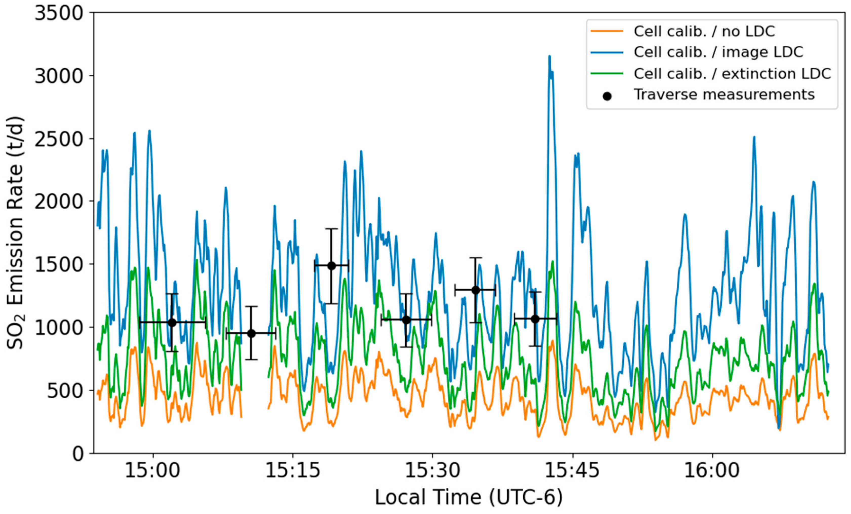
3.3. Results from 13 January 2018

Uncorrected cell-calibrated camera-measured emission rates average 436 metric tons per day (t/d) (

Table 1. Average SO₂ emission rates (in metric tons/day) as measured by camera methodologies, with different light dilution corrections (LDC) and traverses for 13 January 2018 for each traverse time interval. An overall average for all measurements from the day is also included.

	Camera Average during Traverse Number							All Data
	1	2	3	4	5	6	Mean Exl. 2	Full Average
Cell-calib./no LDC	446	-	392	456	383	361	408	436
Cell-calib./extinction LDC	781	-	669	779	654	617	700	617
Cell-calib./ image LDC	1357	-	1033	1267	1034	1306	1199	1295
Traverse	1037	954	1487	1056	1294	1065	1188	1149

, Figure 5), which would be low for Masaya volcano [17,65,66,67,68]. The extinction SO₂ exponential falloff model increases the measured emission rate 1.4 times to 617 t/d. Image-based corrected camera-measured emissions, however, are almost three times larger than uncorrected values, with a mean emission rate of 1295 t/d. Our six traverses are most comparable to the image-based correction, being 11% lower than the image-based correction methodology, but 86% larger than the extinction-based correction. They average 1149 t/d with a standard deviation of 201 t/d. However, the traverses do not cover the entire period of the camera measurements. We can instead compare the time-averaged SO₂ emission rate measured by the camera over the duration of each traverse, weighted to the center of the traverse, taking the travel time of the plume into account. In this comparison, individual traverses can differ from the image-based corrected camera-measured emissions by as much as 40%, though the overall average shows good agreement, within 1%.

Traverse emission rates show less variation than the camera based fluxes. This is expected, as the traverses take several minutes to complete, effectively averaging volcanic emissions over their duration. There are also far fewer traverse measurements than camera data points.

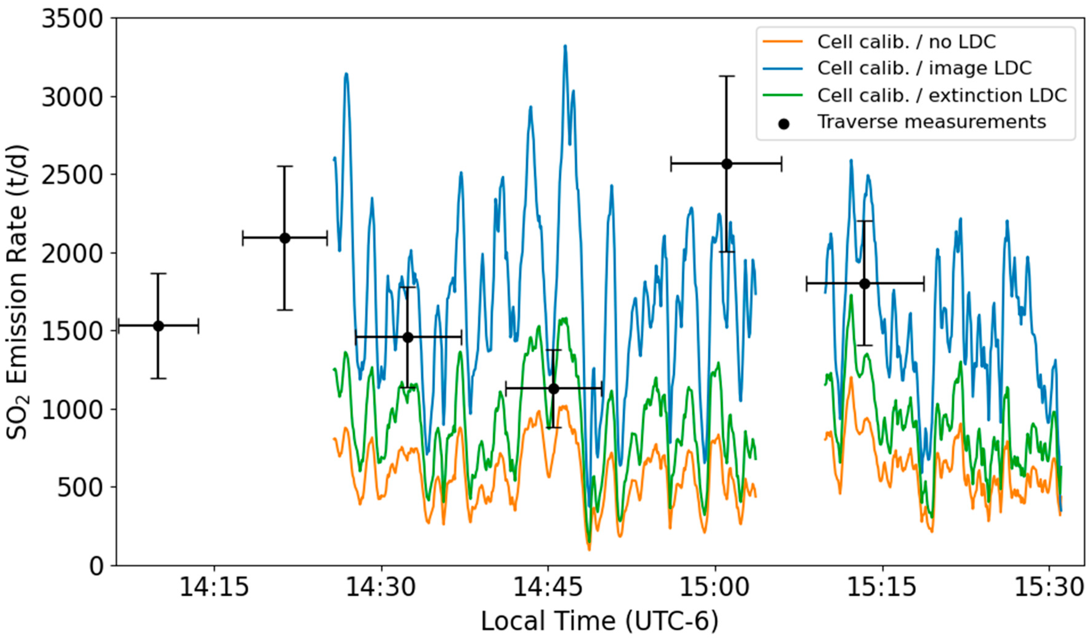
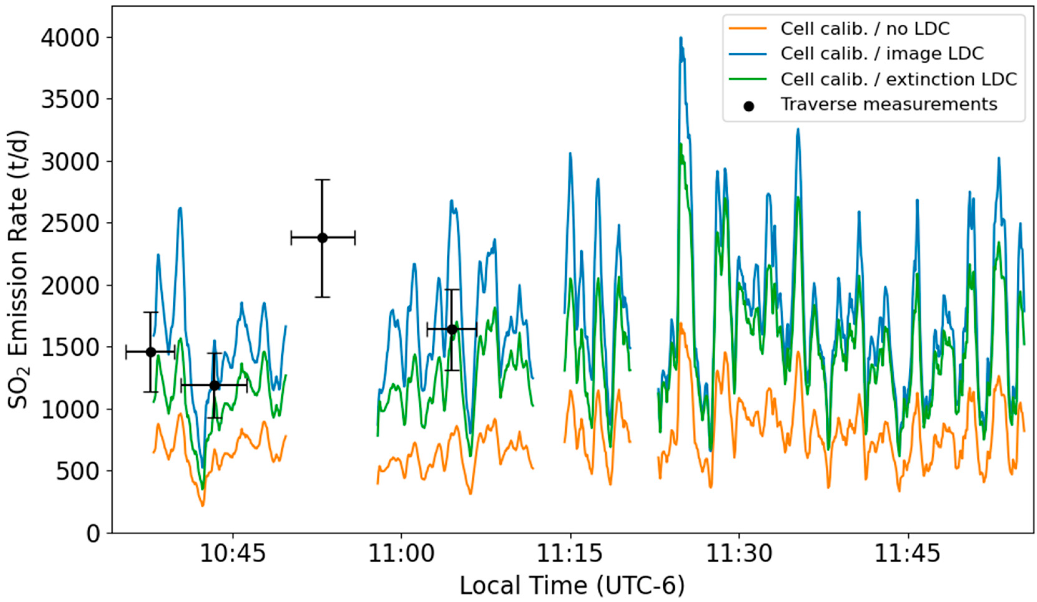
3.4. Results from 10 January 2018

Our measurements of emission rate were moderately higher on the 10th compared to the 13th. Uncorrected camera-measured emissions yielded 589 t/d, which was again much lower than both the average corrected camera-measured emission rates of 1662 t/d and our six traverse averages of 1761 ± 512 t/d (

Table 2. Average SO₂ emission rates (in metric tons/day) as measured by camera methodologies, with different light dilution corrections (LDC) and traverses for 10 January 2018 for each traverse time interval. An overall average for all measurements from the day is also included.

	Camera Average during Traverse Number							All Data
	1	2	3	4	5	6	Mean Exl. 1,2	Full Average
Cell-calib./ no LDC	-	-	583	750	524	756	653	589
Cell-calib./ extinction LDC	-	-	904	1164	813	1087	992	889
Cell-calib./ image LDC	-	-	1573	2072	1689	1788	1781	1662
Traverse	1528	2091	1455	1126	2566	1802	1737	1761

, Figure 6). When only looking at the SO₂ camera flux during the traverse period, the camera flux is again very similar, differing by only 2.5%. The extinction SO₂ corrected flux is significantly lower than both traverses and the image-based corrected fluxes. Variation is again much greater for the camera measurements than the traverse measurements.

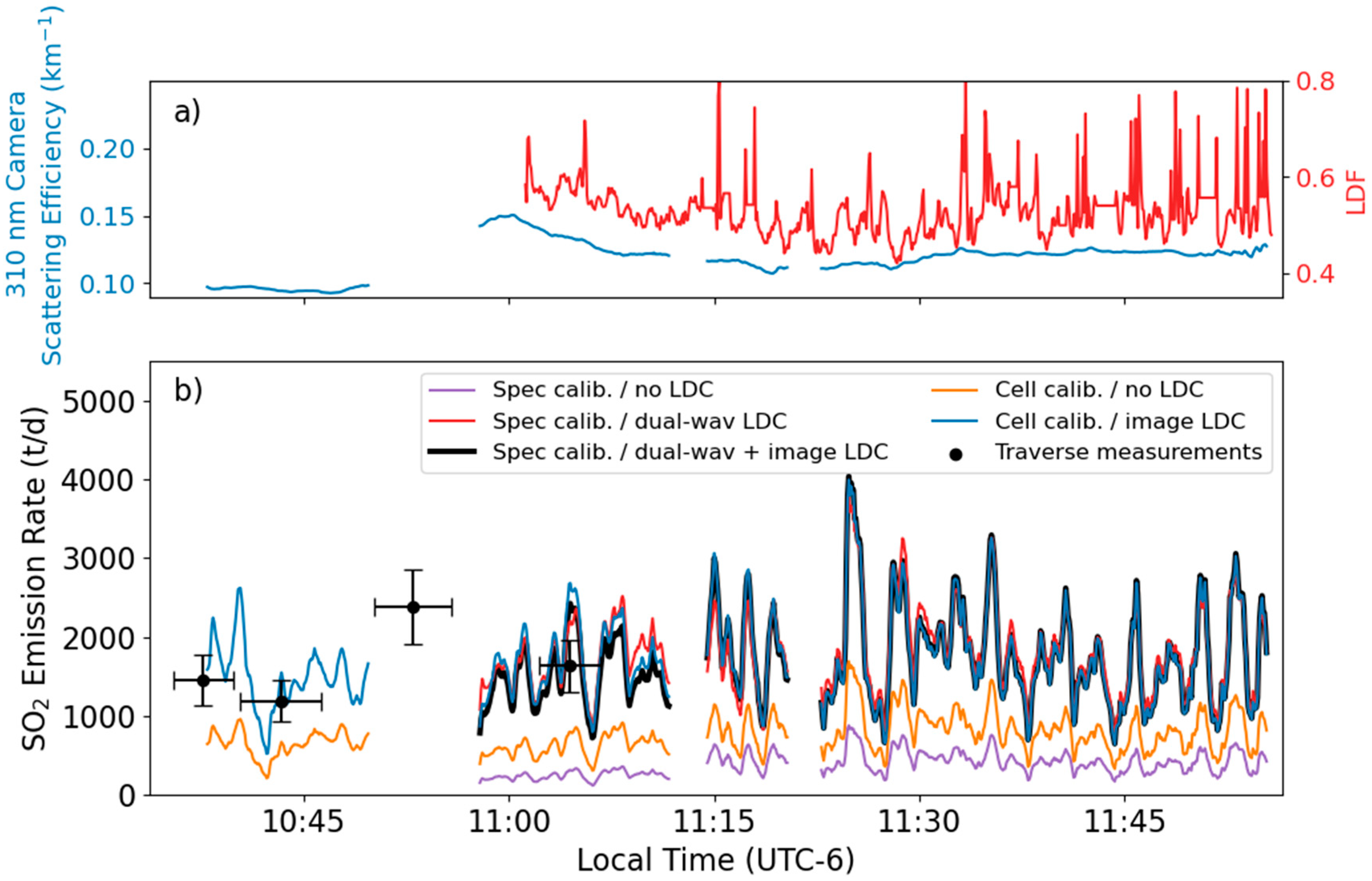
3.5. Results from 15 January 2018

Correction values (light dilution factor and scattering efficiency) show similar changes, though the spectrometer correction light dilution factor (LDF, a measure of scattering) also depends on SO₂ SCD [43], so it is subject to more variation (Figure 7a). A clear difference can be seen between the uncorrected cell-calibrated images (mean 750 t/d) and the spectrometer-calibrated images (mean 384 t/d) (

Table 3. Average SO₂ emission rates (in metric tons/day) as measured by camera methodologies, with different light dilution corrections (LDC) and traverses for 15 January 2018 for each traverse time interval. An overall average for all measurements from the day is also included.

	Camera Average during Traverse Number				All Data
	1	2	3	4	Average from 10:55	Average
Cell-calib./ no LDC	736	540	-	645	772	750
Cell-calib./ extinction LDC	1201	881	-	1278	1448	1376
Cell-calib./ image LDC	1846	1257	-	1914	1757	1709
Spec.-calib./ no LDC	-	-	-	254	384	384
Spec.-calib./ dual-wav LDC	-	-	-	1773	1802	1802
Spec.-calib./ dual-wav LDC + image LDC	-	-	-	1730	1722	1722
Traverse	1459	1186	2377	1637	2007	1665

, Figure 7b). Corrected measurements are more similar, with an overall difference between the methods of 2.5% (image-corrected give 1757 t/d whilst spectrometer-corrected give 1802 t/d for a comparable period). Combining the two light dilution correction techniques, which we suggest is the ideal approach, gives a slightly lower average of 1722 t/d, though still within 5% of the higher spectrometer-corrected only approach. Using the extinction correction, the SO₂ emission rate obtained is again much lower than these other methods (Figure 8). Traverse averages are closest to the combined correction method, giving 1665 ± 510 t/d. However, there were insufficient traverses on this day to adequately sample the plume variation, so it is difficult to definitively say which correction method is most accurate in this case.

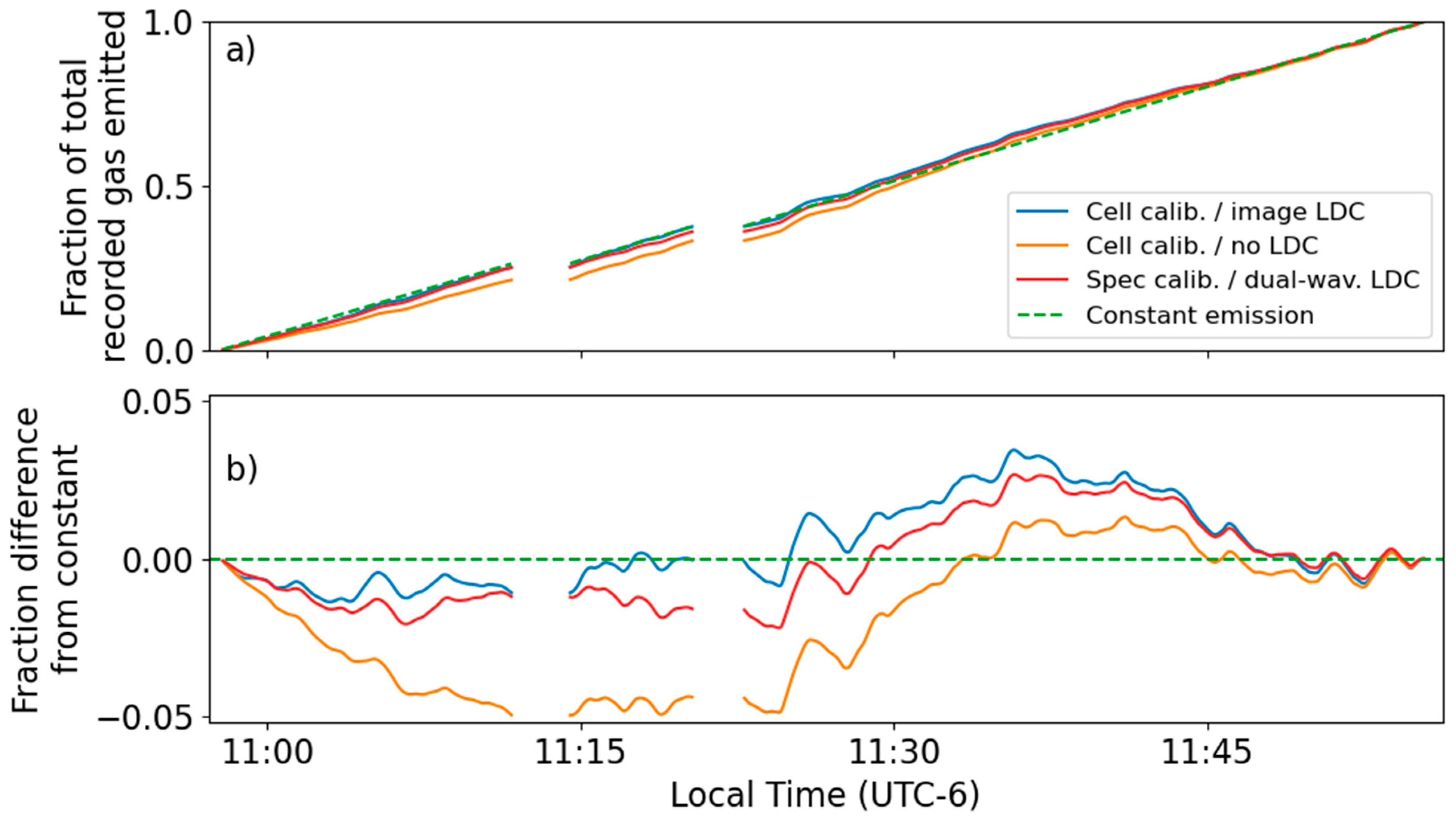
3.6. Cumulative Emissions

Cumulative emissions plots for the three measurement days show constant gradients, modulated by short-term increases and decreases in the flux (Figure 9a,b). This can be seen in both corrected and uncorrected SO₂ emission rates. However, there is a more pronounced curve in the uncorrected emission rate. This would suggest a small change in emission rate across the measurement period. When corrected for light dilution using either method, however, this change in flux is reduced, suggesting a more constant average emission rate.

4. Discussion

Without a light dilution correction, our spectrometer-calibrated SO₂ emission rates measured using the SO₂ camera underestimate the corrected values by approximately 80%. When using cell calibration, the underestimate is reduced to between 55% and 65%. Relative underestimates of the camera and spectrometer may differ in the setup of other researchers depending on the exact camera filters and spectrometer wavelength window used. The extinction light dilution-corrected fluxes also seems to underestimate our corrected values by between 20% to 55%. Our corrected average emission rates are in the range of traverses conducted by INETER within a year of our measurements (2017–2019), which were typically between 600 and 2000 t/d [66,67]. This range is similar to campaign traverse measurements by various groups in 2017, which typically recorded between 800 and 3500 t/d [17,68,69].

For our first two days of measurements (10th and 13th January), there is a good agreement between our camera measurement averages using the image-based correction and the simultaneous traverses (within 2.5%). Since we have used the plume speed as derived from the camera and the wind direction as determined by the traverses, the measurement errors for traverses and camera are likely to be more correlated than usual, making the comparison between the methodologies more accurate. We can, therefore, be confident that the extinction SO₂ correction produces fluxes that are significantly smaller than both traverses and the other corrections. This means the extinction correction does not fully correct for dilution in plumes with SCDs as high as at Masaya.

On the 15th January, we also directly compared the image-based correction with a spectrometer correction for light dilution. These two techniques show good agreement (within 2.5%). This is an encouraging result, since the two methods independently ascertain how diluted the SO₂ SCDs are in the plume. For ideal measurements, we combine both techniques. Explicitly, this means correcting both the camera optical depth and spectrometer SCD for light dilution, then correlating the corrected SCDs with the corrected optical depth to retrieve the correct calibration. As a result, the SO₂ images made with this method have the same SO₂ distributions as is present for the image-based correction. The technique also removes the need for a cell calibration step, and it should perform well even with changing dilution. Using this method, we get an average SO₂ emission rate of 1722 t/d on 15 January 2018.

The range of emission rates measured by the SO₂ camera is substantially larger than that of the traverses. This is because the traverses take time to conduct, so partially average the emission rate across their duration. The large variation in short-term emission rate may be volcanological “puffs”, though at Masaya, there is no link between measured SO₂ flux and lava lake bubble bursts [70]. Consequently, we repeat the possibility that the variation is caused by atmospheric processes, such as wind eddying around the volcanic cone and within the crater. However, the difference between the SO₂ average measured on the 10th and 15th compared to the 13th may be volcanological, though further work would be required to establish any periodicity and a possible cause.

Gas distributions observed by the camera were quite different between the correction methods, with the image-based correction showing a greater SO₂ SCD in the core of the plume and less at the edges. We suggest that the more accurate distribution is from the image-based correction, but the most accurate calibration of this imagery requires light dilution-corrected SO₂ SCDs from a co-located spectrometer. Our combined approach will be particularly useful for studies aiming to partition the SO₂ emission rate between multiple vents or different concurrent degassing styles. There are also differences in the plot of cumulative emission. When not using dilution corrections, the average emission rate appears to change across the measurement period. When using dilution corrections, however, time-averaged cumulative emissions are more consistent. Investigations into degassing periodicities must, therefore, ensure dilution is correctly accounted for to avoid any influence of the lighting or atmospheric conditions artificially creating change across the measurement period.

5. Conclusions

We successfully use traverses to correct the camera for wind direction and use the plume speed measured by the camera as the plume speed for the traverses, improving the reliability of both traverses and camera based flux measurements. Where possible, we recommend that other researchers should use this combined approach to reduce systematic error in their measurements.

We demonstrate a close agreement between two different, independent methods of calibrating the SO₂ camera when correcting for light dilution. These are an improved version of the image-based correction combined with SO₂ cells, and a spectrometer calibration, with the spectrometer readings corrected using dual-waveband modelling. These corrected measurements are larger than the uncorrected measurements by up to a factor of five. Both techniques also closely agree with simultaneous traverses and are significantly greater than simply assuming the SO₂ slant column density decays exponentially with distance.

These calibration methods, however, do produce differences in SO₂ slant column density images. The non-linear correction to optical depth images occurring in the image-based correction is responsible for this difference, producing greater SO₂ slant column densities in the center of the plume, which is of particular importance close to the vent. This difference will affect studies investigating the proportion of gas attributed to “puffing”, explosive and continuous degassing styles. It also affects the trends seen in the cumulative emission rate, here producing a more constant time-averaged flux, which has implications for the timescale of change in degassing at Masaya volcano.

References

1. Malinconico, L.L. Fluctuations in SO2 emission during recent eruptions of Etna. Nature 1979, 278, 43. [Google Scholar] [CrossRef]
2. Daag, A.S.; Tubianosa, B.S.; Newhall, C.; Tungol, N.; Javier, D.; Dolan, M.; Delos Reyes, P.; Arboleda, R.; Martinez, M.; Regalado, T. Monitoring Sulfur Dioxide Emission at Mount Pinatubo. Fire Mud: Erupt. Lahars Mt. Pinatubo Philipp. 1996, 409–414. Available online: https://www.researchgate.net/publication/283364456_Monitoring_sulphur_dioxide_emissions_at_Mount_Pinatubo_Philippines (accessed on 1 March 2021).
3. Burton, M.; Allard, P.; Muré, F.; La Spina, A. Magmatic gas composition reveals the source depth of slug-driven Strombolian explosive activity. Science 2007, 317, 227–230. [Google Scholar] [CrossRef] [Green Version]
4. Symonds, R.B.; Rose, W.I.; Bluth, G.J.S.; Gerlach, T.M. Volcanic-gas studies—Methods, results, and applications. Volatiles Magmas 1994, 30, 1–66. [Google Scholar]
5. Sigurdsson, H.; Houghton, B.; McNutt, S.; Rymer, H.; Stix, J. The Encyclopedia of Volcanoes; Elsevier: Amsterdam, The Netherlands, 2015. [Google Scholar]
6. Platt, U.; Bobrowski, N.; Butz, A. Ground-Based Remote Sensing and Imaging of Volcanic Gases and Quantitative Determination of Multi-Species Emission Fluxes. Geosciences 2018, 8, 44. [Google Scholar] [CrossRef] [Green Version]
7. Burton, M.R.; Oppenheimer, C.; Horrocks, L.A.; Francis, P.W. Remote sensing of CO2 and H2O emission rates from Masaya volcano, Nicaragua. Geology 2000, 28, 915–918. [Google Scholar] [CrossRef]
8. Aiuppa, A.; Giudice, G.; Gurrieri, S.; Liuzzo, M.; Burton, M.; Caltabiano, T.; McGonigle, A.; Salerno, G.; Shinohara, H.; Valenza, M. Total volatile flux from Mount Etna. Geophys. Res. Lett. 2008, 35. [Google Scholar] [CrossRef]
9. Martin, R.; Sawyer, G.; Spampinato, L.; Salerno, G.; Ramirez, C.; Ilyinskaya, E.; Witt, M.; Mather, T.; Watson, I.; Phillips, J. A total volatile inventory for Masaya Volcano, Nicaragua. J. Geophys. Res. Solid Earth 2010, 115. [Google Scholar] [CrossRef]
10. La Spina, A.; Burton, M.; Salerno, G.G. Unravelling the processes controlling gas emissions from the central and northeast craters of Mt. Etna. J. Volcanol. Geotherm. Res. 2010, 198, 368–376. [Google Scholar] [CrossRef]
11. Aiuppa, A.; Cannata, A.; Cannavò, F.; Di Grazia, G.; Ferrari, F.; Giudice, G.; Gurrieri, S.; Liuzzo, M.; Mattia, M.; Montalto, P. Patterns in the recent 2007–2008 activity of Mount Etna volcano investigated by integrated geophysical and geochemical observations. Geochem. Geophys. Geosyst. 2010, 11. [Google Scholar] [CrossRef] [Green Version]
12. Poland, M.P.; Miklius, A.; Sutton, A.J.; Thornber, C.R. A mantle-driven surge in magma supply to Kīlauea Volcano during 2003–2007. Nat. Geosci. 2012, 5, 295–300. [Google Scholar] [CrossRef]
13. Nadeau, P.A.; Werner, C.A.; Waite, G.P.; Carn, S.A.; Brewer, I.D.; Elias, T.; Sutton, A.J.; Kern, C. Using SO2 camera imagery and seismicity to examine degassing and gas accumulation at Kīlauea Volcano, May 2010. J. Volcanol. Geotherm. Res. 2015, 300, 70–80. [Google Scholar] [CrossRef]
14. Salerno, G.G.; Burton, M.; Di Grazia, G.; Caltabiano, T.; Oppenheimer, C. Coupling between magmatic degassing and volcanic tremor in basaltic volcanism. Front. Earth Sci. 2018, 6, 157. [Google Scholar] [CrossRef]
15. McGonigle, A.; Oppenheimer, C.; Galle, B.; Mather, T.; Pyle, D. Walking traverse and scanning DOAS measurements of volcanic gas emission rates. Geophys. Res. Lett. 2002, 29, 46-41–46-44. [Google Scholar] [CrossRef]
16. Edmonds, M.; Herd, R.A.; Galle, B.; Oppenheimer, C.M. Automated, high time-resolution measurements of SO2 flux at Soufriere Hills Volcano, Montserrat. Bull. Volcanol. 2003, 65, 578–586. [Google Scholar] [CrossRef]
17. Stix, J.; de Moor, J.M.; Rüdiger, J.; Alan, A.; Corrales, E.; D’Arcy, F.; Diaz, J.A.; Liotta, M. Using Drones and Miniaturized Instrumentation to Study Degassing at Turrialba and Masaya Volcanoes, Central America. J. Geophys. Res. Solid Earth 2018, 123, 6501–6520. [Google Scholar] [CrossRef]
18. Salerno, G.; Burton, M.; Oppenheimer, C.; Caltabiano, T.; Randazzo, D.; Bruno, N.; Longo, V. Three-years of SO2 flux measurements of Mt. Etna using an automated UV scanner array: Comparison with conventional traverses and uncertainties in flux retrieval. J. Volcanol. Geotherm. Res. 2009, 183, 76–83. [Google Scholar] [CrossRef] [Green Version]
19. Galle, B.; Johansson, M.; Rivera, C.; Zhang, Y.; Kihlman, M.; Kern, C.; Lehmann, T.; Platt, U.; Arellano, S.; Hidalgo, S. Network for Observation of Volcanic and Atmospheric Change (NOVAC)—A global network for volcanic gas monitoring: Network layout and instrument description. J. Geophys. Res. Atmos. 2010, 115. [Google Scholar] [CrossRef]
20. Elias, T.; Kern, C.; Horton, K.A.; Sutton, A.J.; Garbeil, H. Measuring SO2 Emission Rates at Kīlauea Volcano, Hawaii, Using an Array of Upward-Looking UV Spectrometers, 2014–2017. Front. Earth Sci. 2018, 6, 214. [Google Scholar] [CrossRef]
21. Mori, T.; Burton, M. The SO2 camera: A simple, fast and cheap method for ground-based imaging of SO2 in volcanic plumes. Geophys. Res. Lett. 2006, 33. [Google Scholar] [CrossRef]
22. Bluth, G.; Shannon, J.; Watson, I.; Prata, A.; Realmuto, V. Development of an ultra-violet digital camera for volcanic SO2 imaging. J. Volcanol. Geotherm. Res. 2007, 161, 47–56. [Google Scholar] [CrossRef]
23. Burton, M.R.; Prata, F.; Platt, U. Volcanological applications of SO2 cameras. J. Volcanol. Geotherm. Res. 2015, 300, 2–6. [Google Scholar] [CrossRef]
24. Kern, C.; Lübcke, P.; Bobrowski, N.; Campion, R.; Mori, T.; Smekens, J.-F.; Stebel, K.; Tamburello, G.; Burton, M.; Platt, U. Intercomparison of SO2 camera systems for imaging volcanic gas plumes. J. Volcanol. Geotherm. Res. 2015, 300, 22–36. [Google Scholar] [CrossRef]
25. Mori, T.; Burton, M. Quantification of the gas mass emitted during single explosions on Stromboli with the SO2 imaging camera. J. Volcanol. Geotherm. Res. 2009, 188, 395–400. [Google Scholar] [CrossRef]
26. Smekens, J.-F.; Burton, M.R.; Clarke, A.B. Validation of the SO2 camera for high temporal and spatial resolution monitoring of SO2 emissions. J. Volcanol. Geotherm. Res. 2015, 300, 37–47. [Google Scholar] [CrossRef]
27. Smekens, J.-F.; Clarke, A.B.; Burton, M.R.; Harijoko, A.; Wibowo, H.E. SO2 emissions at Semeru volcano, Indonesia: Characterization and quantification of persistent and periodic explosive activity. J. Volcanol. Geotherm. Res. 2015, 300, 121–128. [Google Scholar] [CrossRef]
28. Kern, C.; Sutton, J.; Elias, T.; Lee, L.; Kamibayashi, K.; Antolik, L.; Werner, C. An automated SO2 camera system for continuous, real-time monitoring of gas emissions from Kīlauea Volcano’s summit Overlook Crater. J. Volcanol. Geotherm. Res. 2015, 300, 81–94. [Google Scholar] [CrossRef]
29. Burton, M.; Salerno, G.; D’Auria, L.; Caltabiano, T.; Murè, F.; Maugeri, R. SO2 flux monitoring at Stromboli with the new permanent INGV SO2 camera system: A comparison with the FLAME network and seismological data. J. Volcanol. Geotherm. Res. 2015, 300, 95–102. [Google Scholar] [CrossRef]
30. D’Aleo, R.; Bitetto, M.; Delle Donne, D.; Tamburello, G.; Battaglia, A.; Coltelli, M.; Patanè, D.; Prestifilippo, M.; Sciotto, M.; Aiuppa, A. Spatially resolved SO2 flux emissions from Mt Etna. Geophys. Res. Lett. 2016, 43, 7511–7519. [Google Scholar] [CrossRef] [PubMed] [Green Version]
31. Delle Donne, D.; Tamburello, G.; Aiuppa, A.; Bitetto, M.; Lacanna, G.; D’Aleo, R.; Ripepe, M. Exploring the explosive-effusive transition using permanent ultraviolet cameras. J. Geophys. Res. Solid Earth 2017, 122, 4377–4394. [Google Scholar] [CrossRef]
32. Pering, T.; Tamburello, G.; McGonigle, A.; Aiuppa, A.; James, M.; Lane, S.J.; Sciotto, M.; Cannata, A.; Patanè, D. Dynamics of mild strombolian activity on Mt. Etna. J. Volcanol. Geotherm. Res. 2015, 300, 103–111. [Google Scholar] [CrossRef] [Green Version]
33. Kern, C.; Kick, F.; Lübcke, P.; Vogel, L.; Wöhrbach, M.; Platt, U. Theoretical description of functionality, applications, and limitations of SO2 cameras for the remote sensing of volcanic plumes. Atmos. Meas. Tech. 2010, 3, 733–749. [Google Scholar] [CrossRef] [Green Version]
34. Tamburello, G.; Aiuppa, A.; Kantzas, E.; McGonigle, A.; Ripepe, M. Passive vs. active degassing modes at an open-vent volcano (Stromboli, Italy). Earth Planet. Sci. Lett. 2012, 359, 106–116. [Google Scholar] [CrossRef] [Green Version]
35. Pering, T.D.; Ilanko, T.; Liu, E.J. Periodicity in Volcanic Gas Plumes: A Review and Analysis. Geosciences 2019, 9, 394. [Google Scholar] [CrossRef] [Green Version]
36. Bobrowski, N.; Kern, C.; Platt, U.; Hörmann, C.; Wagner, T. Novel SO2 spectral evaluation scheme using the 360–390 nm wavelength range. Atmos. Meas. Tech. 2010, 3, 879–891. [Google Scholar] [CrossRef] [Green Version]
37. Kern, C.; Deutschmann, T.; Vogel, L.; Wöhrbach, M.; Wagner, T.; Platt, U. Radiative transfer corrections for accurate spectroscopic measurements of volcanic gas emissions. Bull. Volcanol. 2010, 72, 233–247. [Google Scholar] [CrossRef]
38. Mori, T.; Mori, T.; Kazahaya, K.; Ohwada, M.; Hirabayashi, J.I.; Yoshikawa, S. Effect of UV scattering on SO2 emission rate measurements. Geophys. Res. Lett. 2006, 33. [Google Scholar] [CrossRef]
39. Kern, C.; Deutschmann, T.; Werner, C.; Sutton, A.J.; Elias, T.; Kelly, P.J. Improving the accuracy of SO2 column densities and emission rates obtained from upward-looking UV-spectroscopic measurements of volcanic plumes by taking realistic radiative transfer into account. J. Geophys. Res. Atmos. 2012, 117. [Google Scholar] [CrossRef]
40. Lübcke, P.; Bobrowski, N.; Illing, S.; Kern, C.; Nieves, J.; Vogel, L.; Zielcke, J.; Delgado Granados, H.; Platt, U. On the absolute calibration of SO2 cameras. Atmos. Meas. Tech. 2013, 6, 677–696. [Google Scholar] [CrossRef] [Green Version]
41. Campion, R.; Delgado-Granados, H.; Mori, T. Image-based correction of the light dilution effect for SO2 camera measurements. J. Volcanol. Geotherm. Res. 2015, 300, 48–57. [Google Scholar] [CrossRef]
42. Gliß, J.; Stebel, K.; Kylling, A.; Dinger, A.; Sihler, H.; Sudbø, A. Pyplis–a Python software toolbox for the analysis of SO2 camera images for emission rate retrievals from point sources. Geosciences 2017, 7, 134. [Google Scholar] [CrossRef] [Green Version]
43. Varnam, M.; Burton, M.; Esse, B.; Kazahaya, R.; Salerno, G.; Caltabiano, T.; Ibarra, M. Quantifying Light Dilution in Ultraviolet Spectroscopic Measurements of Volcanic SO2 Using Dual-Band Modeling. Front. Earth Sci. 2020, 8, 468. [Google Scholar] [CrossRef]
44. Ilanko, T.; Pering, T.D.; Wilkes, T.C.; Woitischek, J.; D’Aleo, R.; Aiuppa, A.; McGonigle, A.J.; Edmonds, M.; Garaebiti, E. Ultraviolet Camera Measurements of Passive and Explosive (Strombolian) Sulphur Dioxide Emissions at Yasur Volcano, Vanuatu. Remote Sens. 2020, 12, 2703. [Google Scholar] [CrossRef]
45. Boichu, M.; Oppenheimer, C.; Tsanev, V.; Kyle, P.R. High temporal resolution SO2 flux measurements at Erebus volcano, Antarctica. J. Volcanol. Geotherm. Res. 2010, 190, 325–336. [Google Scholar] [CrossRef] [Green Version]
46. Kraus, S. DOASIS: A Framework Design for DOAS. Ph.D. Thesis, University of Mannheim, Mannheim, Germany, 2006. [Google Scholar]
47. Danckaert, T.; Fayt, C.; Van Roozendael, M.; De Smedt, I.; Letocart, V.; Merlaud, A.; Pinardi, G. QDOAS Software User Manual, Belgian Institute for Space Aeronomy (BIRA-IASB): 2012. Available online: http://uv-vis.aeronomie.be/software/QDOAS/QDOAS_manual.pdf (accessed on 7 October 2020).
48. Esse, B.; Burton, M.; Varnam, M.; Kazahaya, R.; Salerno, G. iFit: A simple method for measuring volcanic SO2 without a measured Fraunhofer reference spectrum. J. Volcanol. Geotherm. Res. 2020, 402, 107000. [Google Scholar] [CrossRef]
49. Esse, B. iFit [Computer Software]. 2019. Available online: https://github.com/benjaminesse/iFit (accessed on 25 June 2020).
50. Rufus, J.; Stark, G.; Smith, P.L.; Pickering, J.; Thorne, A. High-resolution photoabsorption cross section measurements of SO2, 2: 220 to 325 nm at 295 K. J. Geophys. Res. Planets 2003, 108. [Google Scholar] [CrossRef] [Green Version]
51. Gorshelev, V.; Serdyuchenko, A.; Weber, M.; Chehade, W.; Burrows, J. High spectral resolution ozone absorption cross-sections–Part 1: Measurements, data analysis and comparison with previous measurements around 293 K. Atmos. Meas. Tech. 2014, 7, 609–624. [Google Scholar] [CrossRef] [Green Version]
52. Grainger, J.; Ring, J. Anomalous Fraunhofer line profiles. Nature 1962, 193, 762. [Google Scholar] [CrossRef]
53. Platt, U.; Stutz, J. Differential Optical Absorption Spectroscopy Principles and Applications Introduction. Differ. Opt. Absorpt. Spectrosc. Princ. Appl. 2008. [Google Scholar] [CrossRef]
54. Penndorf, R. Tables of the refractive index for standard air and the Rayleigh scattering coefficient for the spectral region between 0.2 and 20.0 μ and their application to atmospheric optics. Josa 1957, 47, 176–182. [Google Scholar] [CrossRef]
55. Vogel, L.; Galle, B.; Kern, C.; Delgado Granados, H.; Conde, V.; Norman, P.; Arellano, S.; Landgren, O.; Lübcke, P.; Alvarez Nieves, J. Early in-flight detection of SO2 via Differential Optical Absorption Spectroscopy: A feasible aviation safety measure to prevent potential encounters with volcanic plumes. Atmos. Meas. Tech. 2011, 4, 1785–1804. [Google Scholar] [CrossRef] [Green Version]
56. Ilanko, T.; Pering, T.D.; Wilkes, T.C.; Choquehuayta, F.E.A.; Kern, C.; Moreno, A.D.; De Angelis, S.; Layana, S.; Rojas, F.; Aguilera, F. Degassing at Sabancaya volcano measured by UV cameras and the NOVAC network. Volcanica 2019, 2, 239–252. [Google Scholar] [CrossRef]
57. Weibring, P.; Swartling, J.; Edner, H.; Svanberg, S.; Caltabiano, T.; Condarelli, D.; Cecchi, G.; Pantani, L. Optical monitoring of volcanic sulphur dioxide emissions—comparison between four different remote-sensing spectroscopic techniques. Opt. Lasers Eng. 2002, 37, 267–284. [Google Scholar] [CrossRef]
58. Arellano, S.; Yalire, M.; Galle, B.; Bobrowski, N.; Dingwell, A.; Johansson, M.; Norman, P. Long-term monitoring of SO2 quiescent degassing from Nyiragongo’s lava lake. J. Afr. Earth Sci. 2017, 134, 866–873. [Google Scholar] [CrossRef] [Green Version]
59. Farr, T.G.; Rosen, P.A.; Caro, E.; Crippen, R.; Duren, R.; Hensley, S.; Kobrick, M.; Paller, M.; Rodriguez, E.; Roth, L. The shuttle radar topography mission. Rev. Geophys. 2007, 45. [Google Scholar] [CrossRef] [Green Version]
60. Virtanen, P.; Gommers, R.; Oliphant, T.E.; Haberland, M.; Reddy, T.; Cournapeau, D.; Burovski, E.; Peterson, P.; Weckesser, W.; Bright, J. SciPy 1.0: Fundamental algorithms for scientific computing in Python. Nat. Methods 2020, 17, 261–272. [Google Scholar] [CrossRef] [PubMed] [Green Version]
61. Peters, N.; Hoffmann, A.; Barnie, T.; Herzog, M.; Oppenheimer, C. Use of motion estimation algorithms for improved flux measurements using SO2 cameras. J. Volcanol. Geotherm. Res. 2015, 300, 58–69. [Google Scholar] [CrossRef]
62. Gliß, J.; Stebel, K.; Kylling, A.; Sudbø, A. Improved optical flow velocity analysis in SO2 camera images of volcanic plumes–implications for emission-rate retrievals investigated at Mt Etna, Italy and Guallatiri, Chile. Atmos. Meas. Tech. 2018, 11, 781–801. [Google Scholar] [CrossRef] [Green Version]
63. Klein, A.; Lübcke, P.; Bobrowski, N.; Kuhn, J.; Platt, U. Plume propagation direction determination with SO2 cameras. Atmos. Meas. Tech. 2017, 10, 979–987. [Google Scholar] [CrossRef]
64. Lopez, T.; Aguilera, F.; Tassi, F.; De Moor, J.M.; Bobrowski, N.; Aiuppa, A.; Tamburello, G.; Rizzo, A.L.; Liuzzo, M.; Viveiros, F. New insights into the magmatic-hydrothermal system and volatile budget of Lastarria volcano, Chile: Integrated results from the 2014 IAVCEI CCVG 12th Volcanic Gas Workshop. Geosphere 2018, 14, 983–1007. [Google Scholar] [CrossRef] [Green Version]
65. de Moor, J.; Kern, C.; Avard, G.; Muller, C.; Aiuppa, A.; Saballos, A.; Ibarra, M.; LaFemina, P.; Protti, M.; Fischer, T. A new sulfur and carbon degassing inventory for the Southern Central American Volcanic Arc: The importance of accurate time-series data sets and possible tectonic processes responsible for temporal variations in arc-scale volatile emissions. Geochem. Geophys. Geosyst. 2017, 18, 4437–4468. [Google Scholar] [CrossRef]
66. INETER. Boletín Anual de Enero a Diciembre 2017; Instituto Nicaragüense de Estudios Territoriales: Managua, Nicaragua, 2018. [Google Scholar]
67. INETER. Boletín Anual Vulcanología 2018; Instituto Nicaragüense de Estudios Territoriales: Managua, Nicaragua, 2019. [Google Scholar]
68. Zurek, J.; Moune, S.; Williams-Jones, G.; Vigouroux, N.; Gauthier, P.-J. Melt inclusion evidence for long term steady-state volcanism at Las Sierras-Masaya volcano, Nicaragua. J. Volcanol. Geotherm. Res. 2019, 378, 16–28. [Google Scholar] [CrossRef]
69. Wilkes, T.C.; Pering, T.D.; McGonigle, A.J.S.; Willmott, J.R.; Bryant, R.; Smalley, A.L.; Mims, F.M., III; Parisi, A.V.; England, R.A. The PiSpec: A low-cost, 3D-printed spectrometer for measuring volcanic SO2 emission rates. Front. Earth Sci. 2019, 7, 65. [Google Scholar] [CrossRef]
70. Pering, T.D.; Ilanko, T.; Wilkes, T.C.; England, R.A.; Silcock, S.R.; Stanger, L.R.; Willmott, J.R.; Bryant, R.G.; McGonigle, A.J. A rapidly convecting lava lake at Masaya Volcano, Nicaragua. Front. Earth Sci. 2019, 6, 241. [Google Scholar] [CrossRef]
Figure 1. After [43]. (a) A map of Masaya volcano showing key measurement locations, the active vent and the approximate location of the gas plume. The inset shows the location of Masaya volcano within Nicaragua; (b) a photo of Masaya volcano showing the measurement conditions on the 15th January, captured at 11:27 local time, with the approximate field of view of the spectrometer (circle) and camera (red square) marked. The closest SO2 camera image for the time of the photo is shown in the field of view box.
Remotesensing 13 00935 g001
Figure 2. (a) Distances to the terrain from the camera calculated from NASA Shuttle Radar Topography Mission (SRTM) data. The distances to the triangulated mesh are rendered at their predicted position within the UV camera field of view. The setup shown is for the 13 January 2018; (b) the retrieved scattering efficiencies for the 310 and 330 nm camera for the whole of the 13th January; (c) the fitting residual of the 310 nm efficiency for the final camera frame, captured at 16:12 local time, as measured by the difference between the actual and predicted intensity of the edifice. A histogram shows the distribution of the residual; (d) the raw 310 nm image captured at 16:12 by the SO2 camera, showing the plume emitted by Masaya (greyscale). In red and blue are the residuals shown in (c) as plotted on the edifice.
Remotesensing 13 00935 g002
Figure 3. Calibrations for the conversion between uncorrected SO2 camera optical depth and SO2 slant column density (SCD) for the section of image a spectrometer is viewing, both corrected (blue) and uncorrected (orange) for light dilution, analyzed in the 306–316 nm wavelength window. The legend shows the gradient m from the best fit to the equation y = mx + c. Spectrometer data is from 15 January 2018 from 11:22 to 11:55 am local time. The calibration obtained from measuring SO2 gas cells is also shown (green).
Remotesensing 13 00935 g003
Figure 4. A single SO2 camera image captured on 15 January 2018 at 11:35 local time, as calibrated and corrected using the different methods. White, blue and red dashed lines show the plume speed correlation lines; (a) shows the results from using cell calibration without dilution correction; (b) is from calibrating the SO2 camera using an uncorrected spectrometer, with the correlated field of view of the spectrometer plotted as a red circle; (c) shows the SO2 image produced by correcting the optical depth images for light dilution then using the cell calibration; (d) is the image calibrated using a light dilution-corrected spectrometer, again with the correlated field of view shown. The correlation for this circle is separate to that of (b), producing the different sized circle. Note the change in SO2 distribution between the two corrected SO2 images; (e) the SO2 SCD found along the blue and red plume speed correlation lines in (c) and (d) are plotted for easy comparison of the plume distribution. These SCDs have been corrected for residual in the image optical depth.
Remotesensing 13 00935 g004
Figure 5. Uncorrected (orange), extinction (green) and image-based (blue) light dilution-corrected (LDC) SO2 emission rate from 13 January 2018 as measured by the SO2 camera, with using the cell calibration. Simultaneous traverse emission rates, shown in black, are plotted at the time measured at the center of mass of the traverse minus the travel time from SO2 camera measurement line to traverse road. The traverse error accounts for the duration of the traverse and the error in plume speed estimate from the camera.
Remotesensing 13 00935 g005
Figure 6. Uncorrected (orange), extinction (green) and image-based (blue) light dilution-corrected (LDC) SO2 emission rate from 10 January 2018 as measured by the SO2 camera. Simultaneous traverse emission rates, shown in black, are plotted at the time measured at the center of mass of the traverse minus the travel time from SO2 camera measurement line to traverse road. The traverse error accounts for the duration of the traverse and the error in plume speed estimate from the camera.
Remotesensing 13 00935 g006
Figure 7. (a) Scattering efficiency for the image-based correction (blue) and the light dilution factor (LDF) for the spectrometer correction (red) plotted for the duration of the measurement period on the 15 January 2018; (b) spectrometer-calibrated (purple and red) and cell-calibrated SO2 emission rates (orange and blue) for processed camera data. The spectrometer-calibrated emission rate has been light dilution-corrected (LDC) using dual-waveband modelling (red), whilst the cell-calibrated emission rate had been light dilution-corrected using an image-based correction. Our suggested methodology of combining spectrometer calibration (dual-waveband corrected) with image-based corrections is shown as the thick black line. Traverse measurements (black points with error bars) are also shown as a reference.
Remotesensing 13 00935 g007
Figure 8. Uncorrected (orange), extinction (green) and image-based (blue) light dilution-corrected (LDC) SO2 emission rate 15 January 2018 as measured by the SO2 camera. Simultaneous traverse emission rates, shown in black, are plotted at the time measured at the center of mass of the traverse minus the travel time from SO2 camera measurement line to traverse road. The traverse error accounts for the duration of the traverse and the error in plume speed estimate from the camera.
Remotesensing 13 00935 g008
Figure 9. (a) The cumulative fraction of the total SO2 emission measured by each technique on the 15 January 2018 through each camera frame. Uncorrected (orange), cell-calibrated image-based corrected (blue) and spectrometer-calibrated dual-waveband corrected (red) techniques are presented. Additionally shown is a theoretical constant gas emission through time (green dashes). (b) The difference between the three techniques in (a) and the constant gas emission line.
Remotesensing 13 00935 g009