On the Spectral and Polarimetric Signatures of a Bright Scatterer before and after Hardware Replacement

Abstract

A previous study has used the stable and peculiar echoes backscattered by a single “bright scatterer” (BS) during five winter days to characterize the hardware of C-band, the dual-polarization radar located at Monte Lema (1625 m altitude) in Southern Switzerland. The BS is the 90 m tall metallic tower on Cimetta (1633 m altitude, 18 km range). In this note, the statistics of the echoes from the BS were derived from other ten dry days with normal propagation conditions in winter 2015 and January 2019. The study confirms that spectral signatures, such as spectrum width, wideband noise and Doppler velocity, were persistently stable. Regarding the polarimetric signatures, the large values (with small dispersion) of the copolar correlation coefficient between horizontal and vertical polarization were also confirmed: the average value was 0.9961 (0.9982) in winter 2015 (January 2019); the daily standard deviations were very small, ranging from 0.0007 to 0.0030. The dispersion of the differential phase shift was also confirmed to be quite small: the daily standard deviation ranged from a minimum of 2.5° to a maximum of 5.3°. Radar reflectivities in both polarizations were typically around 80 dBz and were confirmed to be among the largest values observed in the surveillance volume of the Monte Lema radar. Finally, another recent 5-day data set from January 2020 was analyzed after the replacement of the radar calibration unit that includes low noise amplifiers: these five days show poorer characteristics of the polarimetric signatures and a few outliers affecting the spectral signatures. It was shown that the “historical” polarimetric and spectral signatures of a bright scatterer could represent a benchmark for an in-depth comparison after hardware replacements.

1. Introduction

Identification and elimination of ground clutter is a prerequisite for the use of weather radar. Dual-polarization weather radars operating in mountainous terrains, such as the European Alps, are in charge of the surveillance of complex-orography regions. As a consequence, they are necessarily installed on the top of a mountain. Hence, the rejection of ground clutter is critical since good radar visibility from a high site implies a very large number of ground clutter echoes. In the operational radar processing chain of MeteoSwiss, ground clutter is automatically detected using well-consolidated algorithms and then rejected so that only the radar echoes originated by the weather are retained. In this context, the use of high range resolution, Doppler and dual-polarization information maximizes the probability of having at least some clutter-free radar bins for each Cartesian pixel of the resampled operational product in the sampling volumes close to the terrain. One of the first successful efforts to automatically discriminate ground-clutter from precipitation echoes was conceived by Geotis and Silver [1]. A sophisticated and efficient way to combine all the information available concerning radar returns (hence, including the aforementioned statistical tests) is the decision tree algorithm, combined with a dynamic clutter map, as proposed by Joss and Lee [2] (Section 3.d, pages 2623–2624). During several years of operation at the end of the last century, the algorithm has been further improved [3] (Section 2.2, pages 58–63) and better tuned, as shown, for instance, in [4]. Thanks to the clutter-tree approach, it is possible to add new tests in the chain or to change the hierarchical order of the various tests. Consequently, after the installation of five state-of-the-art dual-polarization radars [5], it was possible to introduce in the MeteoSwiss algorithm:

• At the end of the tree, a radar reflectivity static map as a conclusive test for few not-yet-classified bins;
• At the beginning of the tree, a test is based on the polarimetric information.

Regarding the latter point, identifying as weather radial radar bins that show a monotonic increase of the differential propagation phase has resulted in a substantial reduction in the level of residual clutter [5,6,7] and in a smaller number of erroneously canceled weather signals. Regarding the former point, the large and rapid short-term fluctuations of most ground clutter radar bins pose a serious problem in the choice of the “rejection-threshold”. Another example of a decision-tree classifier for the separation of ground clutter from weather targets is the one presented by Steiner and Smith [8]. Alternatively, an effective way for the identification of ground clutter is based on the analysis of the received radar signal in the spectral domain. In this context, one milestone manuscript is the one by Passarelli et al. [9].

Once ground-clutter echoes have been detected, they can be modeled, simulated and studied (e.g., [10,11,12,13]). Thanks to the increase in knowledge and in computational power for modeling and statistical analysis, a novel point of view regarding ground clutter is emerging. It is no longer considered just a disturbance that needs to be rejected. Rather, its spatiotemporal characteristics are instead statistically characterized so that they can be used for monitoring radar hardware. For instance, Silberstein et al. [14] have proposed a relative calibration adjustment (RCA) technique method based on the probability distribution of a clutter area containing hundreds of thousands of ground echoes close to the radar to monitor the stability of radar reflectivity data. The RCA technique was applied to an S-band radar in a tropical oceanic location. Bertoldo et al. [15] have successfully applied a similar approach to an X-band radar in the complex terrain of the Western Alps. The study by Wolff et al. [16] has shown that the RCA technique is well capable of monitoring the reflectivity calibration of other S-band radars, given proper generation of an areal clutter map. In [17], the RCA technique has been modified to work with even higher-frequency radars, including Ka-band cloud radars. The operational implementation of such techniques takes indistinctly into account the reflectivity values of all the ground clutter low range resolution radar bins (typically, 1° × 500 m) that are above a given high reflectivity threshold (e.g., 55 dBz) for more than a given percentage of the time. It considers neither other important spectral and polarimetric information characterizing ground clutter bins nor performs a statistical analysis of individual radar bins. That is why it was proposed to analyze in detail the spectral and polarimetric information associated with an individual “bright scatterer” (BS) [18]. There, it was shown that the peculiar Doppler and polarimetric signatures of the BS distinctively emerge in one single, high-range-resolution radar bin: for the Swiss radar, its sampling volume, which is a function of the antenna half-power beamwidth (HPBW) and the pulse length, corresponds approximately to 1° × 1° × 83.3 m. The analyzed BS target is a 90 m high metallic tower that is located on Cimetta at 1633 m altitude (same altitude as the Monte Lema radar) and 18 km range from Monte Lema. In this note, a statistical characterization of the echoes from the BS during fifteen dry winter days is presented. Detailed information regarding the radar hardware and a description of the BS is given in Section 2, which also briefly describes what kind of spectral and polarimetric signatures could be expected from the BS based on the experience of the previous study [18]. Section 3 presents and describes the results, which are based on the analysis of three 5-day sets in winter with normal propagation conditions. The findings and their implications are discussed in Section 4. Conclusions and possible future analyses are presented in Section 5.

2. Materials and Methods

2.1. The Dual-Polarization Radar Located on Monte Lema at 1625 m Altitude

The Monte Lema radar, which is located at 1625 m altitude 10 km northwest of Lugano, is one of the five identical, dual-polarization, Doppler, C-band (5.5 GHz) systems operated by MeteoSwiss [6]. Antenna-mounted, fully-digital receivers are key aspects of the current network. Each system is equipped with two receiving channels, which are able to simultaneously measure both orthogonal polarization states. Thanks to the receiver-over-elevation design, the waveguide paths of the two receiving channels are almost perfectly symmetric. The advantage of simultaneously transmitting and receiving both polarizations is that the dual-polarization quantities are directly determined from the same transmitted pulse. The main disadvantage is that cross-polar echoes cannot be measured. The two (vertical and horizontal) polarization chains consist, in turn, of two amplifying channels, which are necessary to provide an overall dynamic range better than 95 dB: for each polarization, these two amplification stages (with individual dynamic range much better than 70 dB) are called “high-sensitivity channel” and “low-sensitivity channel”. The latter is typically almost identical to the former one; it is just preceded by a stable, high-quality, low-noise attenuator of approximately 28 dB. In other words, for both polarizations, two channels are combined with a dynamic offset of about 28 dB in order to expand the overall dynamic range. Roughly speaking, the “high-sensitivity channel” can operate between −110 dBm and −40 dBm, while the “low-sensitivity channel” can operate between −80 dBm and −10 dBm. The transition is at around −50 dBm. In order to guarantee system stability and reproducibility, relative calibration of the radar receiver using internal microwave equipment is implemented. In the approach at MeteoSwiss, internal relative calibration is at the highest possible temporal resolution, automatic and independently performed for both polarization channels. It is performed using an internal noise source signal, which is inserted every 5 min at the entrance of the (vertical and horizontal polarization) low noise amplifiers (LNAs) of the low-sensitivity-channel [19] (approximately −90 dBm at such reference injection plane). Since at first approximation, the calibration signal (CAL) delivered by the noise source can be considered constant, a change of the level in terms of analog to digital units (adu) at the output of the digital receiver can be attributed to the LNAs: an increasing temperature causes, in fact, a decreased output, because of the efficiency drops of the amplifier. Absolute calibration of the whole radar refers to the electrical/electromagnetic tuning of the system versus some known reference target at various ranges, e.g., a metal sphere or other reflectors with known radar cross-sections. This requires detailed knowledge of the whole system, including losses of the receiver and transmitter chains, antenna gain, radome losses, noise factor, matched filter losses, atmospheric attenuation, etc. Apart from a few experiments during the site acceptance tests using a radar target simulator [20], the absolute calibration of both transmit and receive chains is not envisaged in the MeteoSwiss network. Nevertheless, absolute calibration accuracy of the (vertical and horizontal polarization) receive chains is checked on-demand, typically a few times per year using the Sun and the methodology presented in [21]. Each MeteoSwiss radar performs plan position indicator scans at 20 interleaved elevations from −0.2° to 40° in 5 min (see [6] for a detailed description of the Swiss scan strategy). The bright scatter (BS) on Cimetta is hit using the lowest angle of elevation; the pulse repetition frequency is 600 Hz. The antenna takes 20 s for a 360° rotation and 1/18 s for an angle of 1°, which is the half-power beamwidth of the antenna radiation pattern; this means that each BS echo (observed every 5 min) is the results of the spectral analysis of 600/18 ≅ 33 pulses.

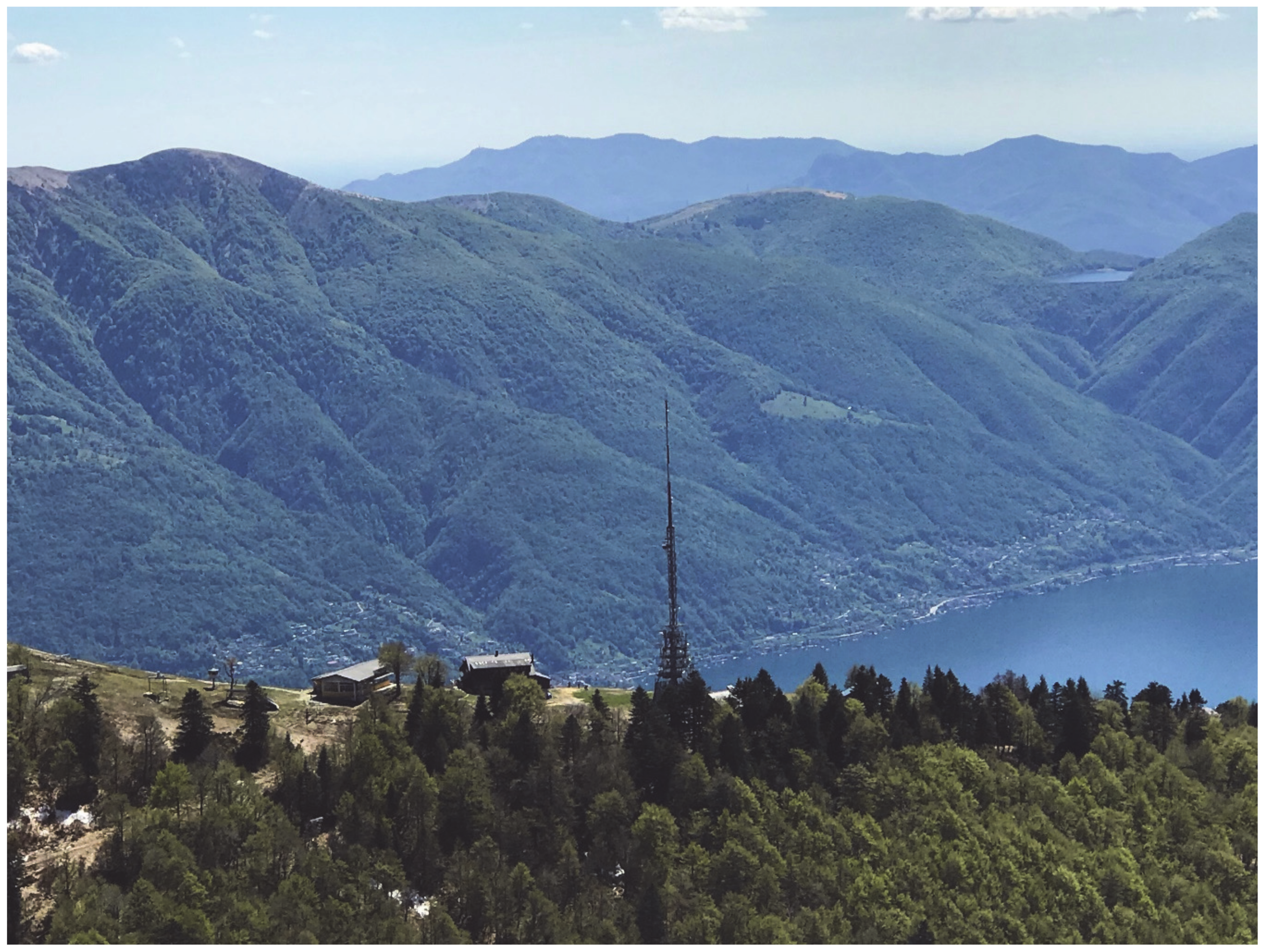
2.2. The Metallic Tower on Cimetta at 1633 m Altitude: A Peculiar Bright Scatterer

Since the half-power beamwidth of the MeteoSwiss radars is 1°, at the range of Cimetta (~18.14 km, the center of the radar bin), the angular resolution of the radar cell is ~314 m (elevation and azimuth). The range resolution of the cell is ~83.33 m. The picture in Figure 1 and the text in Section 2.3 in [18] present in detail the mountainous backscattering environment that characterizes the radar bin, which contains the tall metallic tower. It is by far the dominant scatterer within the radar bin; when it is (azimuthally) hit by the beam axis is practically orthogonal to the incident electromagnetic energy (angle of Elevation of −0.2°). At the base, it is as large as 12 × 12 m and is covered by solar panels. Between 6 and 12 m height there is all sort of telecommunication and broadcasting antennas, then it gets thinner, and it reaches a height of 90 m above the ground (~1633 m altitude): hence, it is not small compared to the half-power beamwidth, and it cannot be assumed to act as a point target. As stated, such a target exhibits a very large radar cross-section and acts as a dominant target within a background of randomly distributed scatterers. A typical radar reflectivity value of the tower plus the background is of the order of 81 dBz, which corresponds (for the Monte Lema horizontal polarization chain) to approximately −18 dBm. The BS signals thus go through the low-sensitivity channel with the 28 dB attenuator.

2.3. Physical Radar Observables Used to Characterize the Bright Scatterer

Details regarding the physical meaning of the moments used in this study (as well as their quantization) can be found in Section 2.2 of [18]. In the following four subsections, we just briefly summarize the typical statistical properties of such moments in the case of a bright scatter.

2.3.1. Spectral Moments: Doppler Spectrum Width and Mean Radial Velocity, Wideband Noise Index

For both spectrum width and wideband noise index, a perfectly stable and constant value was expected. Regarding the Doppler mean radial velocity, we think that in practice, DN values between 126 and 129 could be acceptable (radial velocity close to zero, see Section 3.2 in [18]).

2.3.2. The Copolar Correlation Coefficient

A very important quantity measured by dual-polarization radar is the correlation between the copolar horizontal, HH, and vertical VV returns, called the copolar correlation coefficient (often referred to as ρ_HV or ρ_co). For a detailed and clear description of the rather complicated nature of this variable, the interested reader may refer to the electronic supplement (e06.1) accompanying the book by Fabry [22]. Here it is sufficient to remind that, being the module of the complex correlation coefficient between two orthogonal components (represented by two complex numbers) of the backscattered electromagnetic field within the radar sampling volume, it ranges between 0 (no correlation between the two polarizations) and 1 (perfect correlation). If targets within the radar sampling volume were similar, then the time series of signals at horizontal and vertical polarizations would be highly correlated. On the contrary, the greater the variability in shapes of the targets, the smaller will be the value of ρ^HV. When many backscatterers are randomly distributed within the backscattering sampling volume, the copolar correlation coefficient is considered a measurement of shape diversity. Consequently, the echoes of light rain and drizzle (small and similar spherical drops) are associated with very large values of ρ^HV, mostly larger than 0.995; ρ^HV values in melting snow are lower (typically between 0.8 and 0.9) and make the melting layer easily distinguishable. If the sampling volume contains a significant number of different targets, such it happens with ground clutter, ρ^HV will decrease considerably. In particular, the range of most ground clutter echoes is between 0.650 and 0.950, while the radar bin that contains the Cimetta BS is typical of a dominant scatterer with a huge radar cross-section (that is, the tall metallic tower) within a random uniform background. Hence, very large values of ρ^HV are expected with a left-skewed probability distribution function characterized by a small dispersion. During the five days presented in [18], the average value of ρ^HV resulted in being as large as 0.9962.

2.3.3. The Differential Phase Shift between the Two Orthogonal Polarizations

Another polarimetric quantity measured by the dual-polarization radar is the differential phase shift, Ψ_dp, between the phase of the copolar signal at horizontal and vertical polarization, respectively. This difference between the phase of the two orthogonal polarizations arises from two sources:

• A difference in the delay introduced by the scattering of the transmitted wave, known as the backscattering phase shift, δ_co;
• A difference in the forward propagation velocity of the two polarizations, known as the differential propagation phase, Φ_dp.

In formulas, the differential phase delay, Ψ_dp, at any given range is:

$${\mathsf{\Psi }}_{\mathrm{d}\mathrm{p}}={\mathsf{\delta }}_{\mathrm{c}\mathrm{o}}+{\mathsf{\Phi }}_{\mathrm{d}\mathrm{p}}+{\mathrm{\Psi }}_{\mathrm{0}}$$

(1)

which is the sum

• Of the backscattering phase delay of targets at that range;
• Of the two-way differential propagation phase that occurred when propagating from the radar to the observed target and then back to the radar;
• Of an offset value Ψ₀, which is the phase difference between the two transmit vertically and horizontally polarized waves at range zero.

This last constant value depends on the radar hardware components and design; during dry days also Φ_dp does not vary and can be assumed to zero. Hence, what is observed when analyzing the dispersion of Ψ_dp, is basically the dispersion of the differential backscattering phase shift. For most ground clutter targets, the dispersion is very large, being its distribution uniformly distributed between 0° and 360° (a standard deviation of 360°/12^0.5 would be expected). On the contrary, in the case of the Cimetta BS, the daily dispersion is small: during the five days presented in [18], for instance, the daily standard deviation of Ψ_dp was ~4° in four days out of five (see Section 3.6 in [18]).

2.3.4. Horizontal and Vertical Polarization Reflectivity; Differential Reflectivity

The first (and probably principal) meteorological quantity measured by weather radar in the history of radar meteorology is the so-called radar reflectivity. The backscattered power caused by the hydrometeors and detected by the radar is, in fact, directly proportional to the radar reflectivity, z; the conventional unit of z is a bit awkward: [z] = mm⁶/m³. Since both detected power and radar reflectivity span several order of magnitude, they are often expressed using a Log-transformed scale, after having divided the physical quantity by a normalization factor, since the Log-transformed value must be unit-less. For linear power, P, the normalization value is typically P₀ = 1 mW; similarly, the normalization value for the reflectivity is Z₀ = 1 mm⁶/m³. MeteoSwiss radars can simultaneously measure two orthogonal reflectivities in terms of polarization, which will be indicated as z_h and z_v in linear units or Z_h and Z_v after the Log-transformation. As explained, [z_h] = [z_v] = mm⁶/m³, while [Z_h] = [Z_v] = dBz.

The differential radar reflectivity, Z_dr, is an important polarimetric quantity that can be derived by combining these two observable in a differential manner: it is defined as the Log-transformed ratio between the copolar linear reflectivity measured using horizontal (z_h) and vertical (z_v) polarizations. In formulas:

$$Z_{dr}=10Log\left(z_{h/}{z}_v\right).$$

(2)

The differential reflectivity is expressed in dB, and a value of 0 dB means that z_h = z_v. In practice, Z_dr can also be computed as the difference between Z_h and Z_v. The differential reflectivity was introduced by Seliga and Bringi [23] for a better estimate of rainfall since it contributes to reducing the uncertainty associated with raindrop size distributions. Indeed, the information associated with Z_dr is remarkable; however, the issue of a proper calibration remains a challenge for successful quantitative precipitation estimation. It is worth noting that the copolar correlation coefficient introduced in Section 2.3.2 is connected with the differential reflectivity: ρ^HV can, in fact, be seen as a measure of the dispersion of the differential reflectivity of the 33 instantaneous backscattered echoes used for each 1° radar bin.

What can be expected in terms of radar reflectivities? During the five days presented in [18], the average values of Z_h and Z_v were as large as 81.49 and 80.27 dBz. The median of the 5 median values was 81.5 (80.5) dBz for the horizontal (vertical) polarization. In each of such five days, the average value of the differential reflectivity was very close to the median value. The minimum (maximum) of the daily average value was +0.8 (+1.8) dB. It is worth noting that a strong signal of 81 dBz at the 18 km range corresponds to a received power of–18 dBm at the entrance of the LNA, which is a level 7 dB smaller than the beginning of saturation.

3. Results

The present Section 3 aims at providing a concise description of the experimental results and their interpretation. It is structured in four subsections corresponding to the four sets of radar observables introduced in Section 2.3.

In general, when analyzing the 5-min power returns, we expect a random scattering pattern that is characterized by rapid, short-term fluctuations [24]. The phase (2nd and the 1st Doppler moment) and the wideband noise index are expected to be stable because, during calm wind days, there are rarely moving objects inside the 314 × 314 × 83.33 m radar cell. The results refer to three sets of five dry days with normal propagation conditions; since the sampling time is 5 min, there are 1440 samples per set. In turn, each 1° × 1° × 83.33 m sample was derived by the radar signal processor using 33 pulses.

3.1. Stability of the Spectral Moments and of the Wideband Noise Index (with Some, Rare, Exception in 2019)

During the five selected days in winter 2015 and in January 2019, results are compliant with expectations: both the spectrum width and the wideband noise (WBN) index are constant. In particular, the WBN is always at its minimum value, which corresponds to a maximum value of the Signal Quality Index. As far as the mean radial Doppler velocity is concerned, the DN is either 127 or 128, values that correspond to a zero velocity.

A slightly different situation is observed during the five selected days in January 2020: regarding Doppler velocity, there are several samples with DN = 126 and DN = 125; there is also one sample with DN = 129 and another one with DN = 124. Furthermore, there is one spectrum width sample with DN = 4 instead of the usual constant one. We are not able to find a reason for such anomalies. Finally, it is nice to see that all WBN samples have the usual 0.1 dB value (DN = 1).

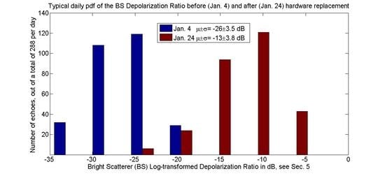
3.2. On the Remarkably Large and Stable Characteristic of the Copolar Correlation Coefficient (But Not in January 2020)

Section 3.2 focuses on the temporal variability of the 288 daily echoes of the radar bin that contains the Cimetta tower in terms of a copolar correlation coefficient.

Table 1. Daily statistical parameters for the copolar correlation coefficient: five days in winter 2015.

	Median	Average	St. Dev.
6 January 2015	0.9954	0.9952	0.0019
7 January 2015	0.9954	0.9952	0.0022
8 January 2015	0.9958	0.9956	0.0018
11 February 2015	0.9972	0.9972	0.0016
12 February 2015	0.9972	0.9968	0.0019

,

Table 2. Daily statistical parameters for the copolar correlation coefficient: five days in January 2019.

	Median	Average	St. Dev.
3 January 2019	0.9987	0.9985	0.0008
4 January 2019	0.9986	0.9985	0.0007
6 January 2019	0.9986	0.9984	0.0008
7 January 2019	0.9985	0.9975	0.0030
8 January 2019	0.9988	0.9986	0.0007

and

Table 3. Daily statistical parameters for the copolar correlation coefficient: five days in January 2020.

	Median	Average	St. Dev.
20 January 2020	0.9773	0.9594	0.0680
21 January 2020	0.9892	0.9812	0.0310
22 January 2020	0.9943	0.9744	0.0627
23 January 2020	0.9947	0.9887	0.0317
24 January 2020	0.9954	0.9812	0.0459

show the daily median, average and standard deviation values for the three selected 5-day sets, all characterized by normal propagation conditions. Both in winter 2015 and in January 2019, results are similar to what has been previously observed. Let us, for instance, consider the average value of ρ_HV obtained in [18], which is 0.9962: it is quite close to the average values that can be obtained by averaging the five values that are listed in the 3rd column of Table 1 and Table 2, namely 0.9961 and 0.9983.

Certainly, the daily values observed in January 2019 are not only particularly large; they are also characterized by a very small dispersion (and a median value very close to the average value) in four days out of five: the only exception is on 7 January 2019, with statistics similar to what observed in winter 2015 (see Table 1 and [18]).

The situation looks very different in January 2020, after the replacement of the LNAs of the low-sensitivity channel: as it can be seen in Table 3, things are quite different both in terms of central locations and dispersion. Regarding the latter, the daily standard deviation of the five days in January 2020 ranges from 0.0310 to 0.0680 (Table 3, last column), while previously its range was between 0.0007 and 0.0030 (Table 1 and Table 2, Table 8 in [18]). As far as the average values are concerned, the average in January 2020 is as low as 0.9770, quite smaller than the above-listed values of 0.9962, 0.9961 and 0.9983. The two days with the largest dispersion (20 and 22 January) are characterized by a remarkably low daily average (0.9594 and 0.9744) and a larger skewness, as can be observed by the difference between the daily median and daily average value. In winter 2015 (Table 1) and January 2019 (Table 2), the maximum difference between median and average is, respectively, 0.0004 and 0.0010, while (Table 3) it results as large as 0.0179 (0.0199) on 20 (22) January 2020.

Adding up, the anomalous and rare differences that were occasionally observed for January 2020 in terms of spectral moments (see Section 3.1) are instead quite statistically significant in the case of the real part of the complex correlation coefficient between the backscattered horizontal and vertical polarizations, namely the copolar correlation coefficient. In the next Section 3.3, the focus will be on the imaginary part of such correlation, which is the differential phase shift.

3.3. On the Small Dispersion of the Differential Phase Shift (But Not in January 2020)

In a previous study, it was shown that the dispersion of the differential phase shift was remarkably small: its daily standard deviation was ~4° in four days. Something similar was observed both in winter 2015 and in January 2019: in the former case, the standard deviation varies from 3.6° to 5.3° (

Table 4. Daily statistical parameters for the differential phase shift. Values are in degrees.

Date	St. Dev.	Date	St. Dev.	Date	St. Dev.
6 January 2015	3.6	3 January 2019	4.2	20 January 2020	44.3
7 January 2015	4.4	4 January 2019	2.5	21 January 2020	47.2
8 January 2015	3.6	6 January 2019	4.4	22 January 2020	76.1
11 February 2015	5.3	7 January 2019	3.6	23 January 2020	28.4
12 February 2015	3.5	8 January 2019	3.6	24 January 2020	28.9

, 2nd column); in the latter case, from a value as small as 2.5° to 4.4° (Table 4, 4th column).

The situation looked very different in January 2020: a deteriorated statistic for the differential phase shift is observed, which is characterized by much larger values of the daily standard deviations: they range, in fact, from a larger than usual value of 28.4° up to an impressive value of 76.1°.

3.4. Some Statistical Characteristic of Radar Reflectivities (and of Differential Reflectivity)

Two parameters that describe the central location of the distribution of the Log-transformed radar reflectivity during the three 5-day sets are shown in

Table 5. Values of two central locations, expected average and median, of the Log-transformed radar reflectivity for the horizontal and vertical polarizations: winter 2015.

Date	E{Zh}	Median{Zh}	Median{Zv}	E{Zv}
6 January 2015	81.31 dBz	81.5 dBz	80.0 dBz	79.58 dBz
7 January 2015	80.28 dBz	80.5 dBz	79.5 dBz	79.20 dBz
8 January 2015	80.89 dBz	81.0 dBz	80.0 dBz	79.69 dBz
11 February 2015	81.57 dBz	82.0 dBz	80.5 dBz	80.24 dBz
12 February 2015	81.26 dBz	81.5 dBz	80.5 dBz	80.31 dBz

,

Table 6. Same as Table 5, but for January 2019.

Date	E{Zh}	Median{Zh}	Median{Zv}	E{Zv}
3 January 2019	82.28 dBz	82.5 dBz	81.5 dBz	81.54 dBz
4 January 2019	82.54 dBz	82.5 dBz	82.0 dBz	81.80 dBz
6 January 2019	81.48 dBz	81.5 dBz	80.5 dBz	80.23 dBz
7 January 2019	81.69 dBz	81.5 dBz	80.5 dBz	80.52 dBz
8 January 2019	81.93 dBz	82.0 dBz	81.0 dBz	80.87 dBz

and

Table 7. Same as Table 5, but for January 2020, after the installation of a different calibration unit.

Date	E{Zh}	Median{Zh}	Median{Zv}	E{Zv}
20 January 2020	73.91 dBz	74.0 dBz	72.5 dBz	72.18 dBz
21 January 2020	73.88 dBz	74.0 dBz	72.0 dBz	71.64 dBz
22 January 2020	73.85 dBz	75.0 dBz	72.0 dBz	71.27 dBz
23 January 2020	74.22 dBz	75.0 dBz	72.0 dBz	71.43 dBz
24 January 2020	75.25 dBz	76.5 dBz	72.0 dBz	71.55 dBz

. The 2nd column and last column show the average of the log-transformed values in dBz, which is the (log of the) geometric average of the linear reflectivity values, for the horizontal and vertical polarization, respectively; the two central columns show the log-transformed median values of the two polarization states. In [18], the median of the 5 median values was 81.5 (80.5) dBz for the horizontal (vertical) polarization. Similar values are observed in winter 2015 and January 2019, namely 81.5 (80.0) dBz and 82.0 (81.0) dBz. Rather smaller values are instead observed in January 2020, especially for the vertical polarization, where the daily median equals 72.0 dBz in four days out of five. In particular, on 23 January, the daily average of the vertical reflectivity is as small as 71.27 dBz.

It is worth noting that in terms of differential reflectivity between the daily median of both polarizations, it results to be 1.5 dB, 2.0 dB, 3.0 dB (twice) and somehow surprisingly as large as 4.5 dB on 24 January 2020 (columns 3 and 4 in Table 7). Writing about the daily average of the differential reflectivity can be easily derived as the difference between the 2nd and the last column of Table 5, Table 6 and Table 7. In [18], the minimum (maximum) of the daily average value was +0.8 (+1.8) dB. On 7 February (6 January), 2015, the minimum (maximum) daily difference occurs: +0.95 (+1.73) dB. In January 2019, the minimum (maximum) of the daily average value was +0.74 (+1.25) dB. Unfortunately, remarkable larger values were observed in January 2020: on 20 January 2020, it is already +1.73 dB; then, it increases day-by-day to reach the maximum value of +3.70 dB on 24 January 2020.

Hence, the statistical parameters of five days in January 2020 are remarkably different from those of the other three 5-day data sets also as far as differential reflectivity and reflectivity are concerned. The frequent and large drops in the copolar correlation coefficient values are associated with an average ~8–9 dB drop in the reflectivity values of the vertical polarization and to a (smaller, but still large) ~6–7 dB drop of the horizontal polarization. Consequently, the daily average differential reflectivity raises from slightly positive values (~1 dB) to a much larger offset of ~3–4 dB.

Adding up, polarimetric and (to a lesser extend) spectral signature of the BS during a 5-day (1440 samples) data set in January 2020 are significantly different from what has been observed during other three similar data sets in previous years. In the next section, we will discuss the hypothesis that this fact could have been caused by a change in the hardware that has occurred in summer 2019.

4. Discussion

In a previous study based on five days with normal propagation conditions [18], the following spectral and polarimetric constraints were set up as a benchmark for future BS echoes during other winter days with normal propagation conditions:

• Spectrum width perfectly stable and null Doppler velocity (DN = 127 or 128);
• Daily median value of the copolar correlation coefficient larger than 0.993.
• Daily median of the horizontal and vertical polarization reflectivity values expected to be inside the [79.5–83.5] and [77.5–82.5] intervals.

In Section 3, we have seen that other “old” five days in winter 2015, as well as other “recent” five days in January 2019, thoroughly and easily satisfy the above-mentioned constraints. Unfortunately, the other five normal propagation days in January 2020 show quite different spectral and polarimetric signatures.

On one hand, meteorological parameters, propagation conditions, hardware monitoring parameters during the five consecutive days in January 2020 are not significantly different from the three sets of 15 days of the previous years. Consequently, the possibility that the observed changes in polarimetric signatures of the BS are caused by environmental factors can reasonably be excluded. On the other hand, in summer 2019, a new calibration unit (CU), which includes four low-noise amplifiers (LNAs), was installed. Hence, such a different and awkward response of the Cimetta BS during 2020 could be related to the new configuration of low-sensitivity LNAs. Investigations and discussions with the manufacturer are ongoing.

Having said that daily polarimetric statistics of the Cimetta BS in January 2020 are unsatisfactory, an alternative approach could be that of limiting the statistics to observation periods shorter than a diurnal cycle, but at least long enough to collect several tens of samples. This approach leads to the following question: during such five days, is it possible to find some sub-period (say, at least seventy samples, ~6 h) with polarimetric signatures similar to those of the previous years?

The answer is affirmative for two important polarimetric moments: the copolar correlation coefficient and the differential phase shift. For instance, from 8 UTC to 18 UTC (120 echoes) on 22 January 2020, the median (mean) value of ρ^HV is 0.9954 (0.9916); the standard deviation is a bit larger than the previous year but still with two zeros: 0.0077. A similar expression (a bit larger, but still acceptable) can be used to describe the 10 h standard deviation of the differential phase shift, which results to be 9.3°. As far as the radar reflectivity is concerned, the observed values are not as large as in the past: the median 10 h value is 76 (74) dBz for the horizontal (vertical) polarization. These two median values are larger than the daily ones of 75 (72), but they are still smaller than the two above-mentioned “warning” thresholds. The average 10 h value is 75.7 (73.7) dBz for the horizontal (vertical) polarization. This corresponds to an average 10 h differential reflectivity of 2.0 dB, similar to 20 January (and to the largest value of the past) and smaller than what was obtained in the other four successive days. There are at least other two or three similar sub-periods: here, we just mention the one that lasts from 03 to 14 UTC on 23 January (132 samples): the median (mean) value of ρ^HV is 0.9941 (0.9934); its standard deviation is 0.0035. The 11 h standard deviation of the differential phase shift results to be 8.2°. Hence, the copolar correlation coefficient and the differential phase shift also show statistics similar to the dry winter days of previous years. However, this is not the case as far as the radar reflectivity is concerned: the median 11 h value is 76 (72.5) dBz for the horizontal (vertical) polarization. The average 11 h value is 75.5 (72.6) dBz for the horizontal (vertical) polarization, which corresponds to an average 11 h differential as large as 2.9 dB.

5. Summary, Conclusions and Outlook

Thanks to the exponential increase in computational power for high-resolution, intensive data processing, a new point of view has emerged in recent years regarding ground clutter: its statistics are investigated aiming at monitoring the quality (and stability) of radar hardware. In this note, we repeat a previously presented analysis that deals with spectral and polarimetric (copolar correlation coefficient, differential phase shift, differential reflectivity) information characterize an individual radar bin that contains a dominant target (BS) with deterministic backscattering properties in a background comprised of a random distribution of scatterers.

A data set of 4320 echoes backscattered by the BS during 15 (normal propagation and) dry days in winter 2015 and 2019 (this note and [18]) shows:

• A very small daily standard deviation of the copolar correlation coefficient ρ^HV, which ranges from 0.007 to 0.0030;
• A very large daily average of ρ^HV, which ranges from 0.9939 to 0.9986;
• A very small daily standard deviation of the differential phase shift (E{Ψ_dp} < 9.5°);
• A daily average differential reflectivity between 0.7 dB and 1.9 dB;
• A daily average horizontal reflectivity ranging from 80.28 dBz and 82.54 dBz;
• A daily average vertical reflectivity ranging from 79.20 dBz and 81.54 dBz;

Unfortunately, after hardware replacement, including the two low-sensitivity LNAs for both vertical and horizontal polarizations, larger dispersions and smaller average values occur, as observed using data of five consecutive dry days in January 2020. A more detailed analysis reveals that it is at least possible to select 3 sub-periods (for a total of approximately 30 h out of 120 h) that are characterized by a very large average of ρ^HV and a very small dispersion of both ρ^HV and Ψ_dp. However, the average of the radar reflectivity, although larger than the daily average, remains smaller than the above-listed limits even during such sub-periods, especially regarding the vertical polarization. In turn, the large decrease of the vertical polarization implies an increase of the differential reflectivity: on 24 January 2020, the daily average of Z_dr results to be 3.7 dB (see Table 7, second and last column). However, even during the 7.5 h period that is characterized by typical statistics of ρ^HV and Ψ_dp, Z_dr results to be as large as 4.1 dB.

We conclude that it is possible to use echoes backscattered by a single “bright scatterer” (BS) to characterize the hardware of the dual-polarization radar: our efforts will be toward the identification of other sub-periods during cold, dry days in 2020 with typical past statistics of ρ^HV and Ψ_dp together with careful monitoring of Z_h Z_v and Z_dr. A complementary approach consists of finding other targets with similar polarimetric signatures and noting whether some sort of change took place between January 2019 and 2020, especially as far as polarimetric signatures are concerned. We will certainly go on investigating and discussing with the radar manufacturer regarding the possible causes that affect such BS signatures after hardware replacement: some outliers are occasionally observed in the Doppler spectrum with and WBN. On average, a remarkable decrease of horizontal reflectivity is observed; such a decrease is even larger for vertical polarization, which implies an increased average differential reflectivity. This fact, combined with an average decrease of the copolar correlation coefficient, results in a remarkable deterioration of the depolarization ratio for a simultaneous transmitting and receiving (STAR) system as defined in [25,26], which is a nonlinear combination of ρ^HV and the linear ratio between z_h and z_v. In previous years, a typical average value of this important parameter for the Cimetta BS was, for instance, −19.1 dB (6 January 2015) or −25.9 dB (4 January 2019). After hardware replacement, it results to be, on average, as large as −12.7 dB on 24 January 2020 or −15.9 dB on 22 January 2020. Could this level of depolarization be considered acceptable for the Cimetta bright scatterer?

References

1. Geotis, S.G.; Silver, W.M. An evaluation of techniques for automatic ground-echo rejection. In Proceedings of the 17th Conference on Radar Meteorology, Seattle, WA, USA, 26–29 October 1976; pp. 448–452. [Google Scholar]
2. Joss, J.; Lee, R. The application of radar-gauge comparisons to operational precipitation profile corrections. J. Appl. Meteor. 1995, 34, 2612–2630. [Google Scholar] [CrossRef] [Green Version]
3. Germann, U.; Joss, J. Operational measurement of precipitation in mountainous terrain. In Weather Radar: Principles and Advanced Applications; Meischner, P., Ed.; Springer: Berlin, Germany, 2004; pp. 52–77. [Google Scholar]
4. Gabella, M.; Notarpietro, R. Ground clutter characterization and elimination in mountainous terrain. In Proceedings of the 2nd European Conference on Radar in Meteorology and Hydrology (ERAD2002), Delft, The Netherlands, 18–22 November 2002; pp. 305–311. [Google Scholar]
5. Germann, U.; Boscacci, M.; Gabella, M.; Sartori, M. Radar design for prediction in the Swiss Alps. Meteorol. Technol. Int. 2015, 4, 42–45. [Google Scholar]
6. Friedrich, K.; Germann, U.; Tabary, P. Influence of Ground Clutter Contamination on Polarimetric Radar Parameters. J. Atmos. Ocean. Technol. 2009, 26, 251–269. [Google Scholar] [CrossRef] [Green Version]
7. Panziera, L.; Gabella, M.; Germann, U.; Martius, O. A 12-year radar-based climatology of daily and sub-daily extreme precipitation over the Swiss Alps. Int. J. Climatol. 2018, 1–21. [Google Scholar] [CrossRef]
8. Steiner, M.; Smith, J.A. Use of three-dimensional reflectivity structure for automated detection and removal of non-precipitating echoes in radar data. J. Atmos. Ocean. Technol. 2002, 19, 673–686. [Google Scholar] [CrossRef]
9. Passarelli, R.E.; Romanik, P.; Geotis, S.G.; Siggia, A.D. Ground-clutter rejection in the frequency domain (for radar meteorology applications). In Proceedings of the Preprints of the 20th Conf. on Radar Meteorology, Boston, MA, USA; 1981; pp. 295–300. [Google Scholar]
10. Delrieu, G.; Creutin, J.D.; Andrieu, H. Simulation of radar mountain returns using a digitized terrain model. J. Atmos. Ocean. Technol. 1995, 12, 1039–1049. [Google Scholar] [CrossRef] [Green Version]
11. Gabella, M.; Perona, G. Simulation of the orographic influence on weather radar using a geometric-optics approach. J. Atmos. Ocean. Technol. 1998, 15, 1486–1495. [Google Scholar] [CrossRef]
12. Hubbert, J.C.; Dixon, M.; Ellis, S.M.; Meymaris, G. Weather Radar Ground-clutter. Part I: Identification, Modeling, and Simulation. J. Atmos. Ocean. Technol. 2009, 26, 1165–1185. [Google Scholar] [CrossRef]
13. Hubbert, J.C.; Dixon, M.; Ellis, S.M.; Meymaris, G. Weather radar ground-clutter. Part II: Real-time identification and filtering. J. Atmos. Ocean. Technol. 2009, 26, 1181–1197. [Google Scholar] [CrossRef]
14. Silberstein, D.S.; Wolff, D.B.; Marks, D.A.; Atlas, D.; Pippitt, J.L. Ground Clutter as a Monitor of Radar Stability at Kwajalein, RMI. J. Atmos. Ocean. Technol. 2008, 25, 2037–2045. [Google Scholar] [CrossRef]
15. Bertoldo, S.; Notarpietro, R.; Gabella, M.; Perona, G. Ground clutter analysis to monitor the stability of a mobile X-band radar. In Proceedings of the 9th International Workshop on Precipitation in Urban Areas, St Moritz, Switzerland, 6–9 December 2012; pp. 41–45. [Google Scholar]
16. Wolff, D.B.; Marks, D.A.; Petersen, W.A. General Application of the Relative Calibration Adjustment (RCA) Technique for Monitoring and Correcting Radar Reflectivity Calibration. J. Atmos. Ocean. Technol. 2015, 32, 496–506. [Google Scholar] [CrossRef]
17. Hunzinger, A.; Hardin, J.C.; Bharadwaj, N.; Varble, A.; Matthews, A. An extended radar relative calibration adjustment (eRCA) technique for higher-frequency radars and range–height indicator (RHI) scans. Atmos. Meas. Technol. 2020, 13, 3147–3166. [Google Scholar] [CrossRef]
18. Gabella, M. On the Use of Bright Scatterers for Monitoring Doppler, Dual-Polarization Weather Radars. Remote Sens. 2018, 10, 1007. [Google Scholar] [CrossRef] [Green Version]
19. Vollbracht, D.; Sartori, M.; Gabella, M. Absolute dual-polarization radar calibration: Temperature Dependence and Stability with Focus on Antenna-Mounted Receivers and Noise Source-Generated Reference Signal. In Proceedings of the 8th European Conference on Radar in Meteorology and Hydrology (ERAD2014), Garmisch-Partenkirchen, Germany, 1–5 September 2014. [Google Scholar]
20. Gabella, M.; Sartori, M.; Progin, O.; Germann, U. Acceptance tests and monitoring of the next generation polarimetric weather radar network in Switzerland. In Proceedings of the IEEE International Conference Electromagnetics Advanced Applications, Torino, Italy, 9–13 September 2013. [Google Scholar]
21. Gabella, M.; Boscacci, M.; Sartori, M.; Germann, U. Calibration accuracy of the dual-polarization receivers of the C-band Swiss weather radar network. Atmosphere 2016, 7, 76. [Google Scholar] [CrossRef] [Green Version]
22. Fabry, F. Radar Meteorology: Principles and Practice, 1st ed.; Cambridge University Press: Cambridge, UK, 2015; 256p, ISBN 978-1-107-07046-2. [Google Scholar]
23. Seliga, T.; Bringi, V. Potential use of radar differential reflectivity measurements at orthogonal polarizations for measuring precipitation. J. Appl. Meteor. 1976, 15, 69–76. [Google Scholar] [CrossRef] [Green Version]
24. Ulaby, F.T.; Dobson, M.C. Handbook of Radar Scattering Statistics for Terrain; Artech House: Norwood, MA, USA, 1989; 357p. [Google Scholar]
25. Matrosov, S.Y. Depolarization estimates from linear H and V measurements with weather radars operating in simultaneous transmission–simultaneous receiving mode. J. Atmos. Ocean. Technol. 2004, 21, 574–583. [Google Scholar] [CrossRef]
26. Melnikov, V.; Matrosov, S.Y. Estimations of aspect ratios of ice cloud particles with the WSR-88D radar. In Proceedings of the 36th Conference on Radar Meteorology, Breckenridge, CO, USA, 2013, 16–20 September; Available online: https://ams.confex.com/ams/36Radar/webprogram/Paper228291.html (accessed on 27 February 2021).
Figure 1. Looking south towards Monte Lema from a point an altitude of ~1800 m North of Cimetta; from left to right, the chairlift arrival, the hut and the 90 m tall metallic tower (BS).
Remotesensing 13 00919 g001