
SSCNN-S: A Spectral-Spatial Convolution Neural Network with Siamese Architecture for Change Detection


Abstract
1. Introduction
- (1)
- 1D and 2D convolutional neural networks are used to extract spectral features and spatial features while local tensors are converted into spectral-spatial vectors. In this manner, the spectral and the spatial features are combined to increase detection speed.
- (2)
- (3)
- The four-test scoring method is proposed. This method is mainly used in parameter selection experiments with uncertain results. For each set of parameters, the method can give the final results based on the results of two to four independent experiments as the basis for parameter selection.
2. Materials and Methods
2.1. Establishing the Sample Set
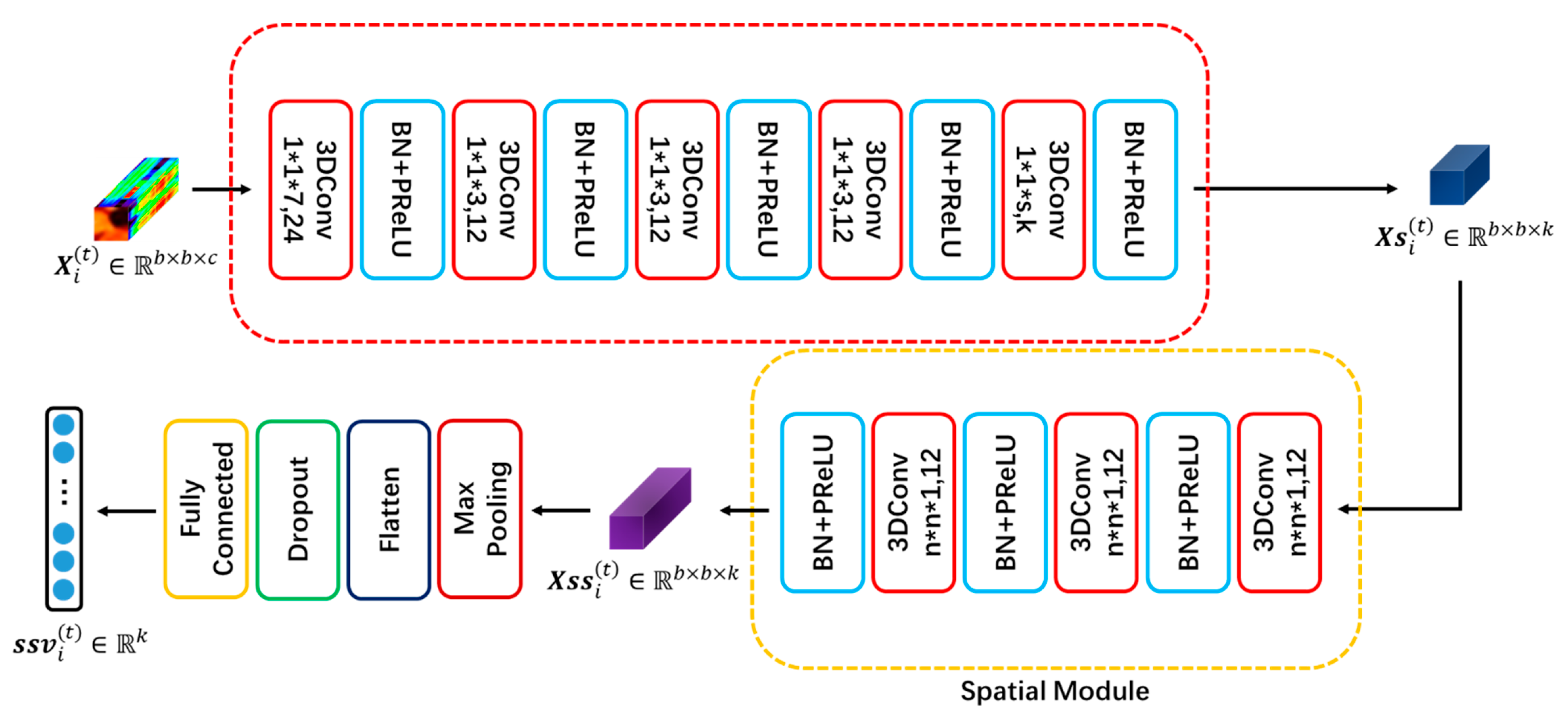
2.2. Extract Spectral-Spatial Features of the Hyperspectral Tensor
2.2.1. Spectral Module
2.2.2. Spatial Module
2.2.3. Achieve Spectral-Spatial Vector
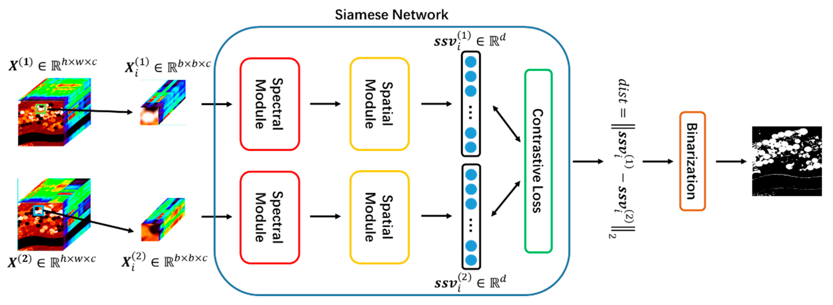
2.3. Contrastive Loss in the Siamese Network
2.4. Proposed SSCNN-S Method
| Algorithm 1: Algorithm of SSCNN-S for hyperspectral image (HSI) change detection (CD). |
| Input: 1. Two HSIs of the same region at different times with ground truthing. 2. The number of training pairs and the number of validation pairs . Step 1: Construct the corresponding tensor sets and for two HSIs and pair them to form a tensor pair and generate the sample set according to the change situation reflected by the ground truthing. Step 2: Randomly select pairs in as the training set and randomly select pairs in as the validation set . Step 3: Input and to the network. Step 4: Train the model and obtain the optimal parameters. Step 5: Traverse all possible thresholds in the validation set to select the optimal threshold . Step 6: Calculate the distance for each pixel. If the distance is greater than , it is considered as a changed pixel; otherwise, it is considered an unchanged pixel. Output: 1. Change map. |
3. Results
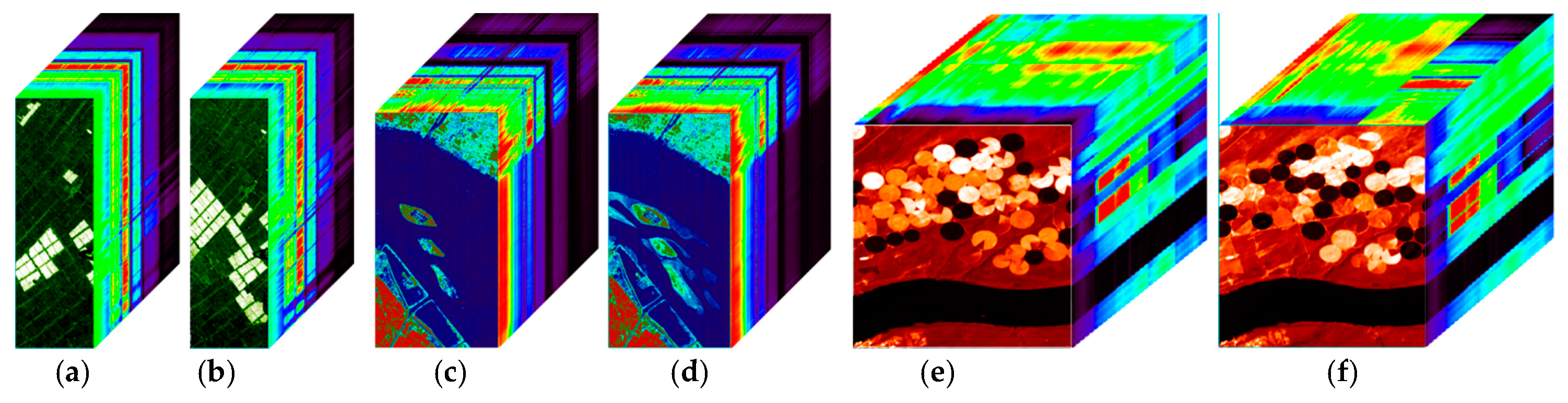
3.1. Data Sets
3.2. Evaluation Index
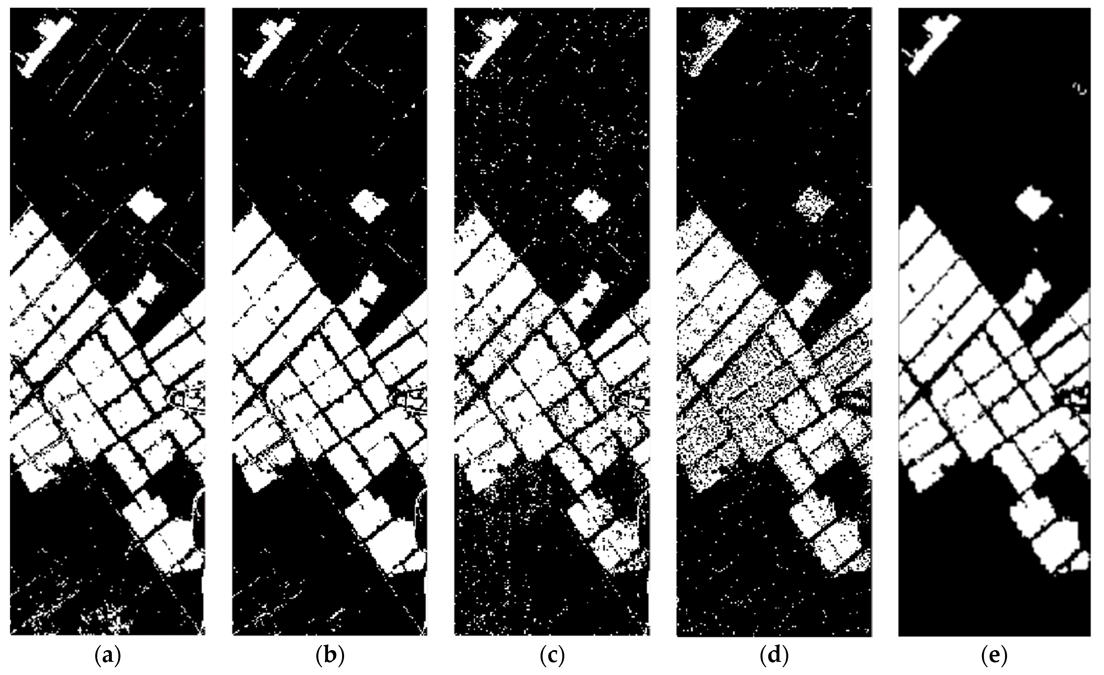
3.3. Experimental Results
4. Discussion
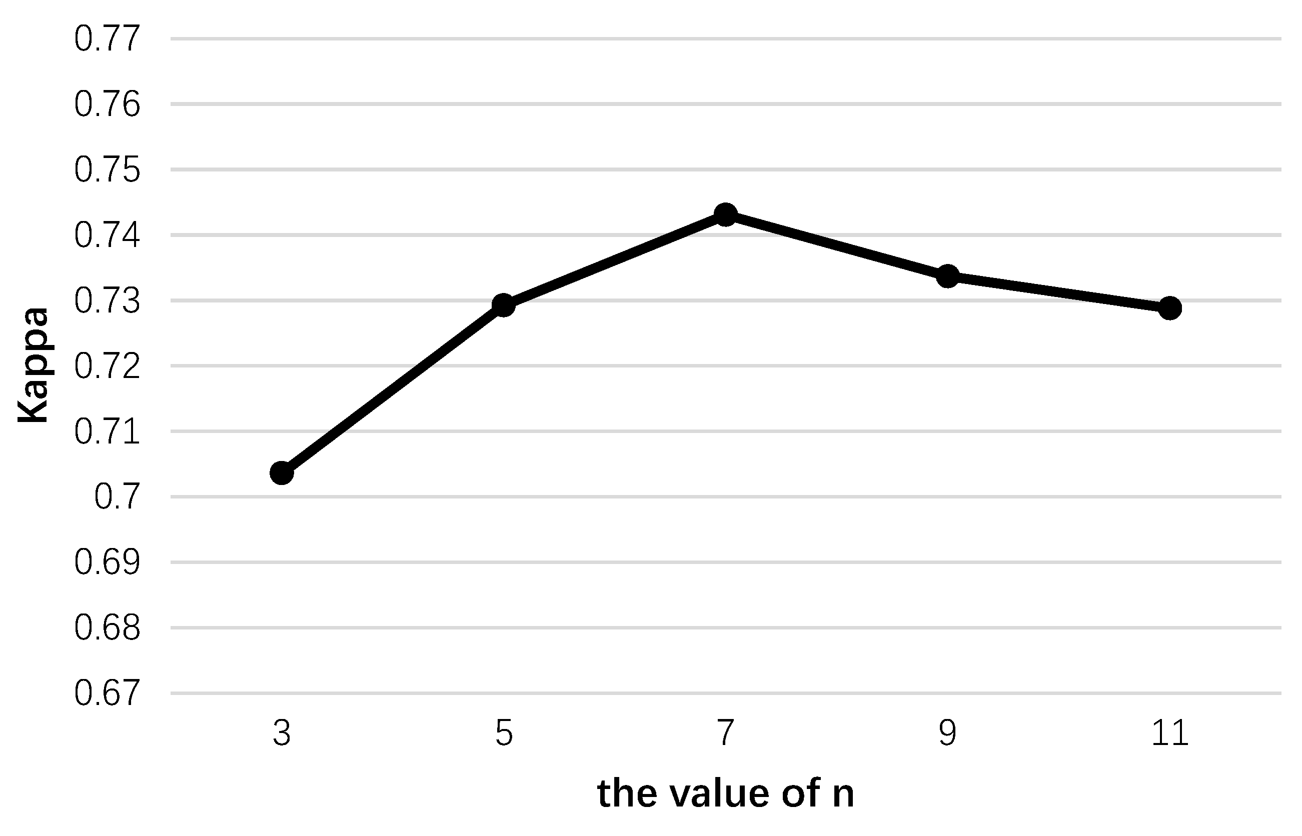
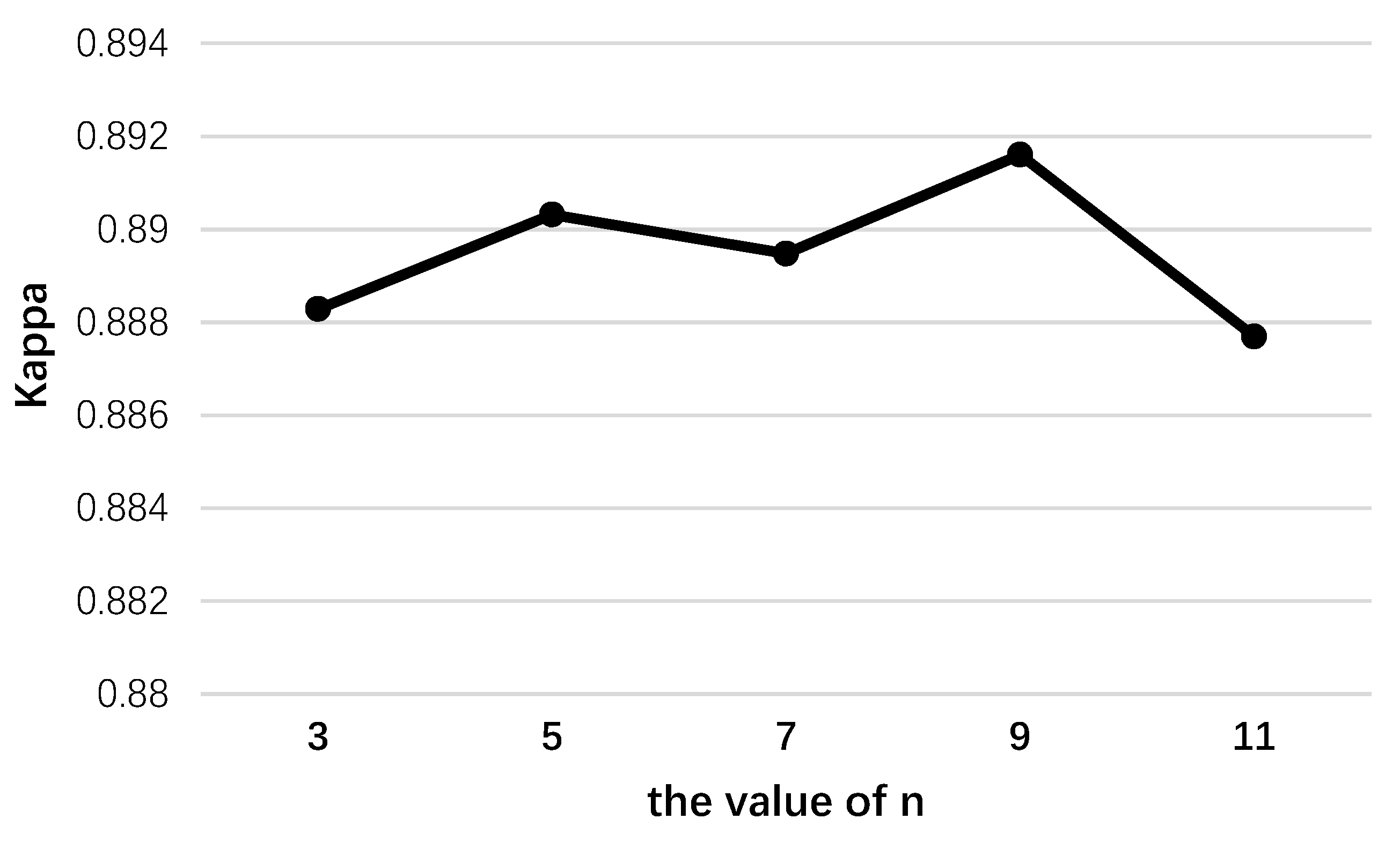
4.1. Selecting Parameters
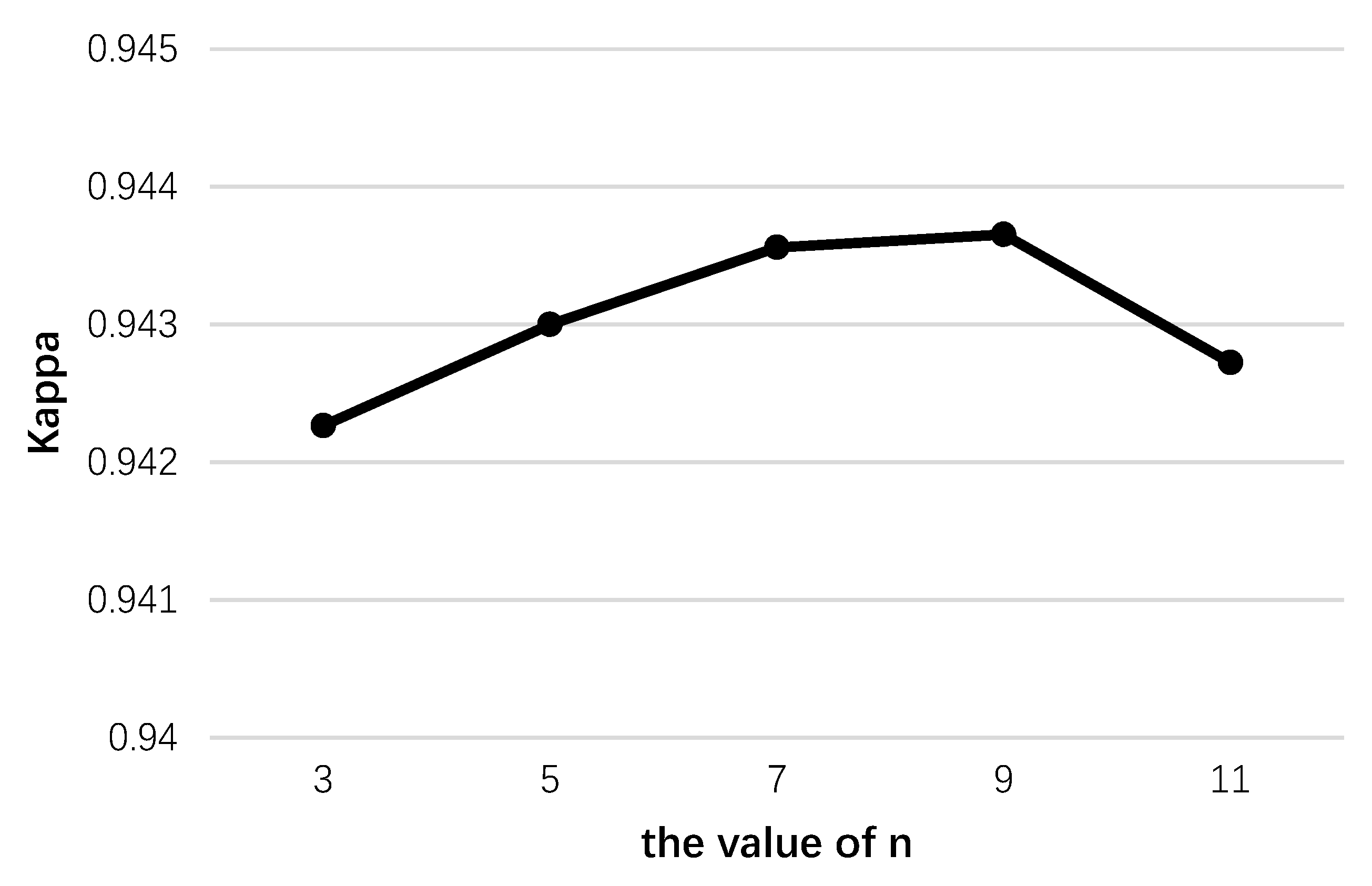
4.1.1. Parameters in the Spectral Module
| Algorithm 2: Four-test scoring method. |
| Input: 1. Error threshold . Step 1: Perform the first experiment and obtain the result . Step 2: Perform the second experiment and obtain the result . Step 3: If , let the final result be . The algorithm is aborted. Step 4: Otherwise, perform the third experiment and obtain the result . Step 5: If , let the final result be . The algorithm is aborted. Step 6: Otherwise, if , let the final result be . The algorithm is aborted. Step 7: Otherwise, perform the final experiment and obtain the result . Step 8: Let the final result be . Output: 1. Final result . |
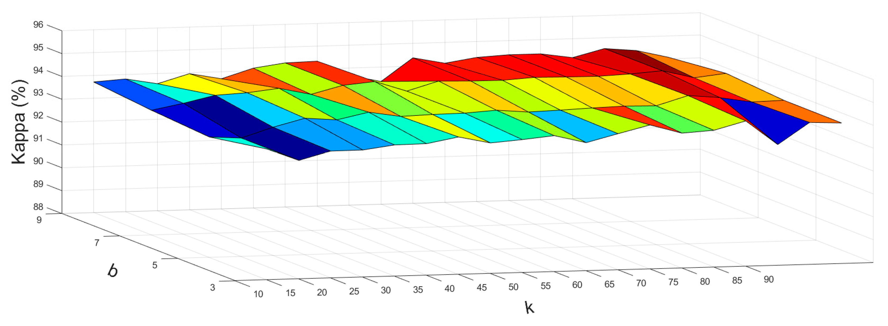
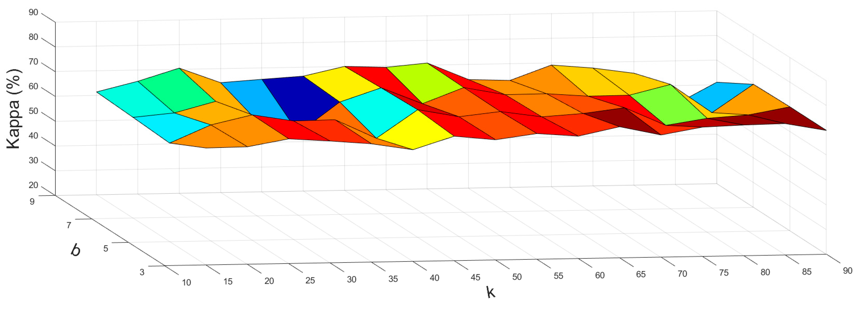
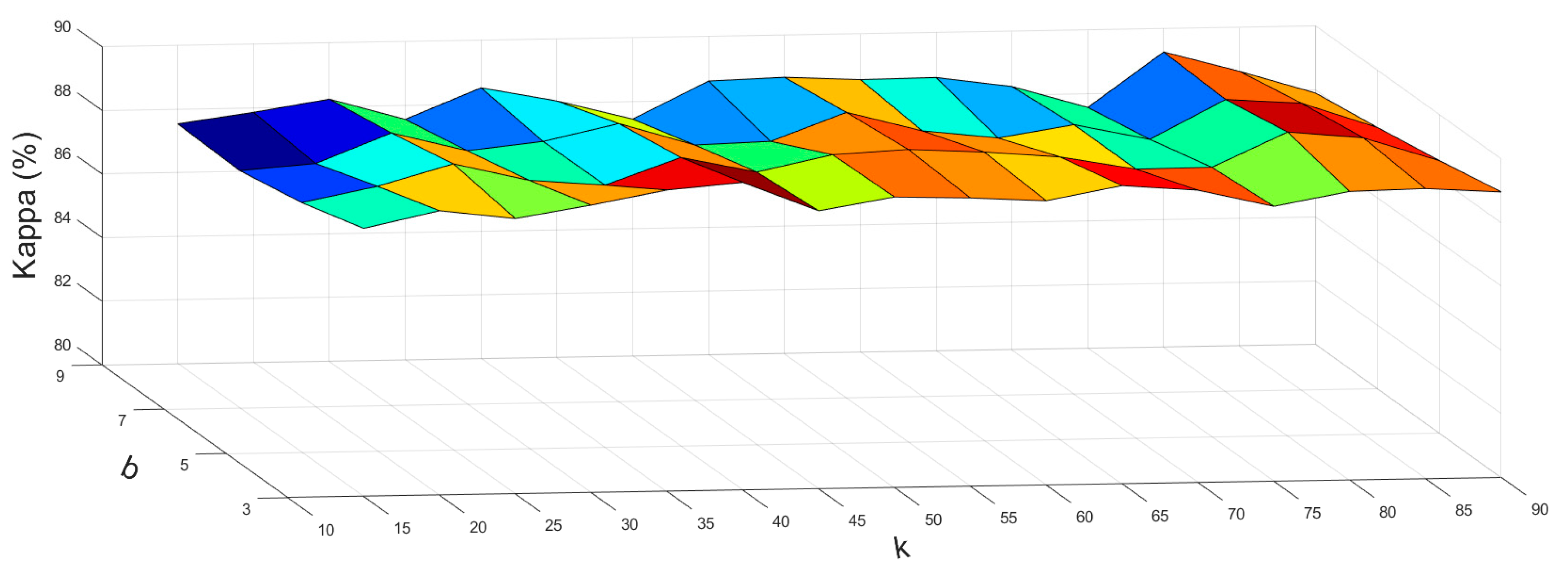
4.1.2. Parameters in the Spatial Module
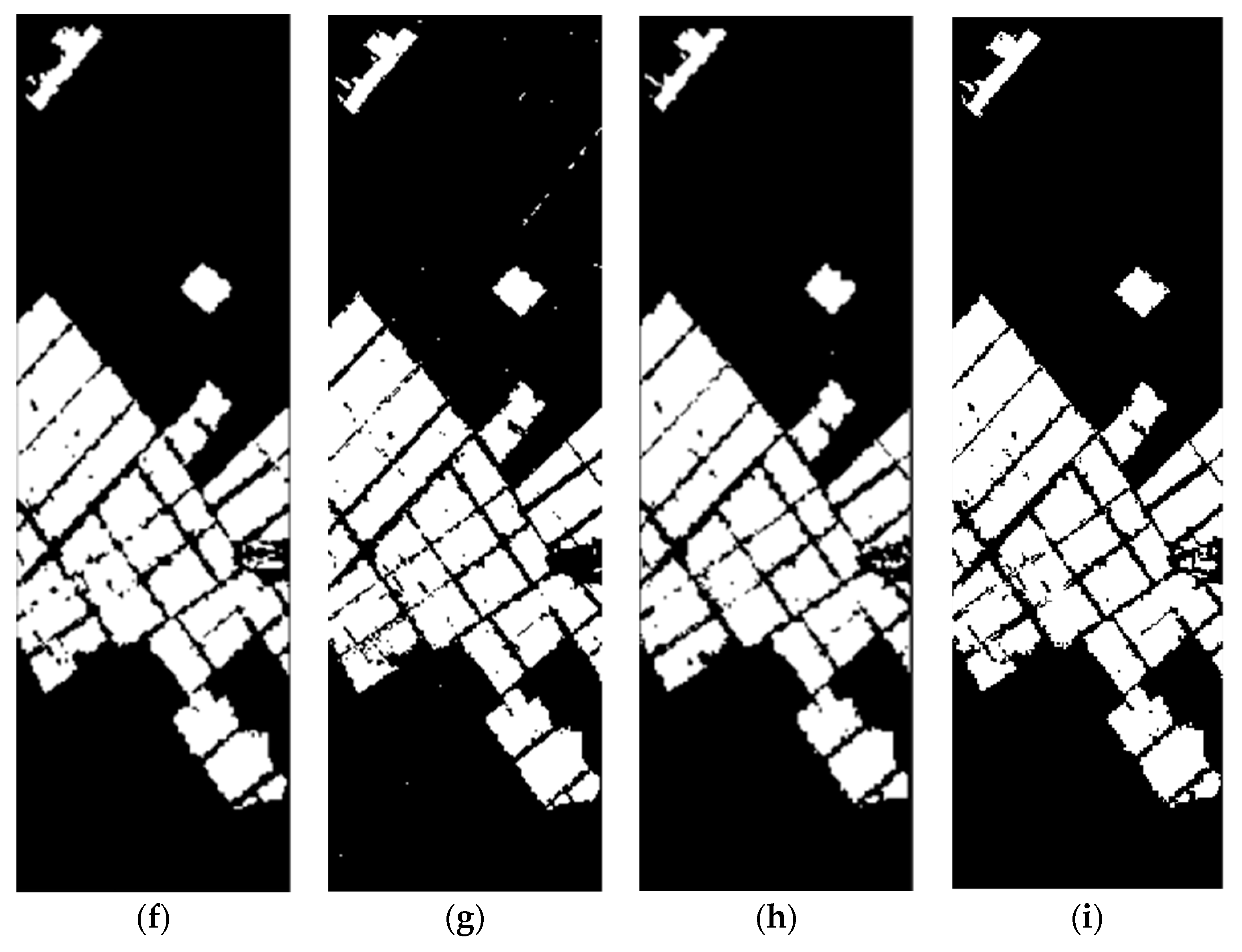
4.2. Discussion on Farmland Experiment
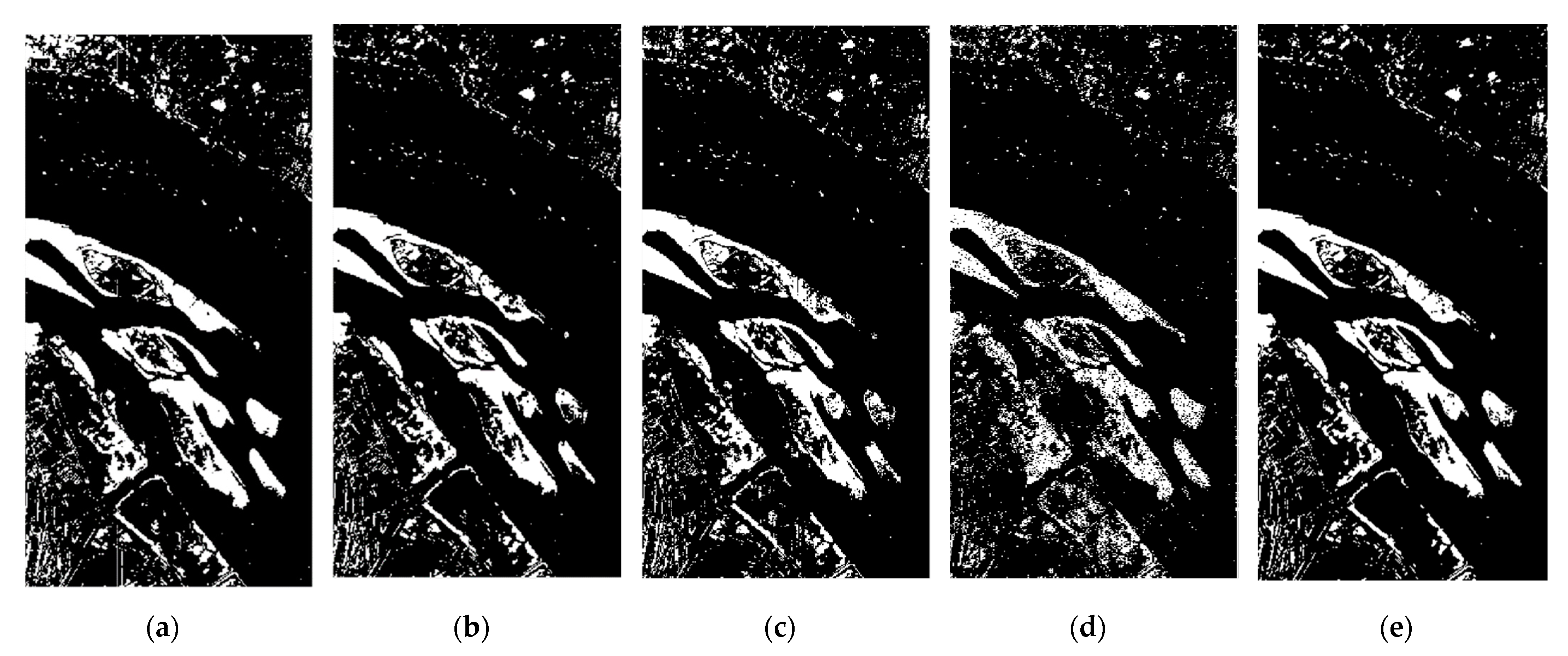
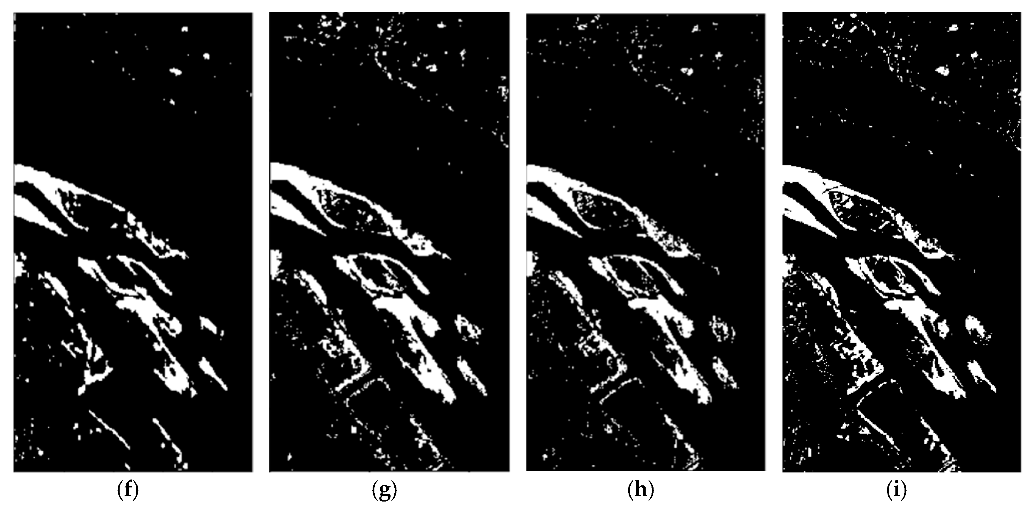
4.3. Discussion on River Experiment
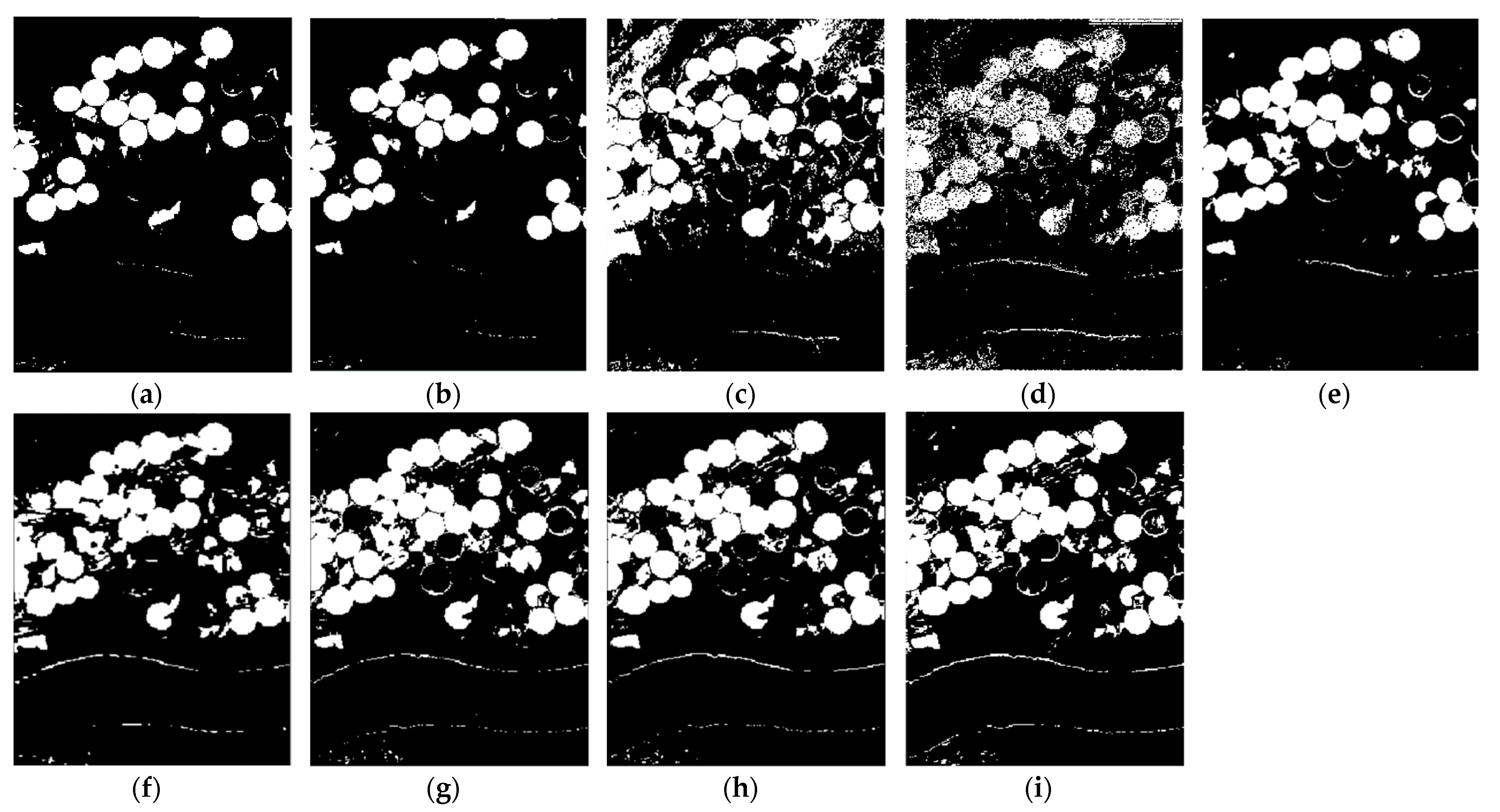
4.4. Discussion on USA Experiment
5. Conclusions
Author Contributions
Funding
Acknowledgments
Conflicts of Interest
References
- Li, Y.; Hu, C.; Ao, D. Rapid surface large-change monitoring by repeat-pass GEO SAR multibaseline interferometry. IEEE Geosci. Remote Sens. Lett. 2020, 1–5. [Google Scholar] [CrossRef]
- Yasir, M.; Sheng, H.; Fan, H.; Nazir, S.; Niang, A.J.; Salauddin, M.; Khan, S. Automatic coastline extraction and changes analysis using remote sensing and GIS technology. IEEE Access 2020, 8, 180156–180170. [Google Scholar] [CrossRef]
- Ansari, R.A.; Buddhiraju, K.M.; Malhotra, R. Urban change detection analysis utilizing multiresolution texture features from polarimetric SAR images. Remote Sens. Appl. Soc. Environ. 2020, 20, 100418. [Google Scholar] [CrossRef]
- Liu, S.; Marinelli, D.; Bruzzone, L.; Bovolo, F. A review of change detection in multitemporal hyperspectral images: Current techniques, applications, and challenges. IEEE Geosci. Remote Sens. Mag. 2019, 7, 140–158. [Google Scholar] [CrossRef]
- Padŕon-Hidalgo, J.A.; Pérez-Suay, A.; Nar, F.; Laparra, V.; Camps-Valls, G. Efficient kernel Cook’s Distance for remote sensing anomalous change detection. IEEE J. Sel. Top. Appl. Earth Obs. Remote Sens. 2020, 13, 5480–5488. [Google Scholar] [CrossRef]
- Wu, C.; Zhang, L.; Du, B. Hyperspectral anomaly change detection with slow feature analysis. Neurocomputing 2015, 151, 175–187. [Google Scholar] [CrossRef]
- Hou, Y.; Zhu, W.; Wang, E. Hyperspectral Mineral Target Detection Based on Density Peak. Intell. Autom. Soft Comput. 2019, 25, 805–814. [Google Scholar] [CrossRef]
- Dalmiya, C.P.; Santhi, N.; Sathyabama, B. A novel feature descriptor for automatic change detection in remote sensing images. Egypt. J. Remote Sens. Space Sci. 2019, 22, 183–192. [Google Scholar] [CrossRef]
- Chen, Z.; Wang, B. Spectrally-spatially regularized low-rank and sparse decomposition: A novel method for change detection in multitemporal hyperspectral images. Remote Sens. 2017, 9, 1044. [Google Scholar] [CrossRef]
- Zhao, J.; Yang, J.; Lu, Z.; Li, P.; Liu, W. Change detection based on similarity measure and joint classification for polarimetric SAR images. In Proceedings of the 2017 IEEE International Geoscience Remote Sensing Symposium (IGARSS), Fort Worth, TX, USA, 23–28 July 2017; pp. 1896–1899. [Google Scholar]
- Wu, C.; Zhang, L.; Zhang, L. A scene change detection framework for multi-temporal very high resolution remote sensing images. Signal. Process. 2016, 124, 184–197. [Google Scholar] [CrossRef]
- Lu, L.; Weng, Q.; Guo, H.; Feng, S.; Li, Q. Assessment of urban environmental change using multi-source remote sensing time series (2000–2016): A comparative analysis in selected megacities in Eurasia. Sci. Total Environ. 2019, 684, 567–577. [Google Scholar] [CrossRef]
- Henrot, S.; Chanussot, J.; Jutten, C. Dynamical spectral unmixing of multitemporal hyperspectral images. IEEE Trans. Image Process. 2016, 25, 3219–3232. [Google Scholar] [CrossRef]
- MALILA, W. Change vector analysis: An approach for detecting forest changes with Landsat. In Proceedings of the Machine Processing of Remotely Sensed Data Symposium, West Lafayette, IN, USA, 29 June–1 July 1980; pp. 326–335. [Google Scholar]
- Nielsen, A.A.; Conradsen, K.; Simpson, J.J. Multivariate alteration detection (MAD) and MAF postprocessing in multispectral, bitemporal image data: New approaches to change detection studies. Remote Sens. Environ. 1998, 64, 1–19. [Google Scholar] [CrossRef]
- Nielsen, A.A. The regularized iteratively reweighted MAD method for change detection in multi-and hyperspectral data. IEEE Trans. Image Process. 2007, 16, 463–478. [Google Scholar] [CrossRef] [PubMed]
- Hardoon, D.R.; Szedmak, S.; Shawe-Taylor, J. Canonical correlation analysis: An overview with application to learning methods. Neural Comput. 2004, 16, 2639–2664. [Google Scholar] [CrossRef] [PubMed]
- Bovolo, F.; Marchesi, S.; Bruzzone, L. A framework for automatic and unsupervised detection of multiple changes in multitemporal images. IEEE Trans. Geosci. Remote Sens. 2011, 50, 2196–2212. [Google Scholar] [CrossRef]
- Nemmour, H.; Chibani, Y. Multiple support vector machines for land cover change detection: An application for mapping urban extensions. ISPRS J. Photogramm. Remote Sens. 2006, 61, 125–133. [Google Scholar] [CrossRef]
- Bruzzone, L.; Liu, S.; Bovolo, F.; Du, P. Change detection in multitemporal hyperspectral images. In Multitemporal Remote Sensing; Springer: Cham, Swizerland, 2016; pp. 63–88. [Google Scholar]
- Liu, S.; Du, Q.; Tong, X.; Samat, A.; Pan, H.; Ma, X. Band selection-based dimensionality reduction for change detection in multi-temporal hyperspectral images. Remote Sens. 2017, 9, 1008. [Google Scholar] [CrossRef]
- Ye, Q.; Yang, J.; Liu, F.; Zhao, C.; Ye, N.; Yin, T. L1-Norm Distance Linear Discriminant Analysis Based on an Effective Iterative Algorithm. IEEE Trans. Circuits Syst. Video Technol. 2018, 28, 114–129. [Google Scholar] [CrossRef]
- Fu, L.; Li, Z.; Ye, Q.; Yin, H.; Liu, Q.; Chen, X.; Fan, X.; Yang, W.; Yang, G. Learning Robust Discriminant Subspace Based on Joint L2,p- and L2,s-Norm Distance Metrics. IEEE Trans. Neural Netw. Learn. Syst. 2020, 1–15. [Google Scholar] [CrossRef] [PubMed]
- Ye, Q.; Li, Z.; Fu, L.; Yang, W.; Yang, G. Nonpeaked Discriminant Analysis for Data Representation. IEEE Trans. Neural Netw. Learn. Syst. 2019, 30, 3818–3832. [Google Scholar] [CrossRef]
- Zhang, H.; Gong, M.; Zhang, P.; Su, L.; Shi, J. Feature-level change detection using deep representation and feature change analysis for multispectral imagery. IEEE Geosci. Remote Sens. Lett. 2016, 13, 1666–1670. [Google Scholar] [CrossRef]
- Ma, L.; Jia, Z.; Yu, Y.; Yang, J.; Kasabov, N.K. Multi-spectral image change detection based on band selection and single-band iterative weighting. IEEE Access 2019, 7, 27948–27956. [Google Scholar] [CrossRef]
- Yu, W.; Zhang, M.; Shen, Y. Learning a local manifold representation based on improved neighborhood rough set and LLE for hyperspectral dimensionality reduction. Signal. Process. 2019, 164, 20–29. [Google Scholar] [CrossRef]
- Xu, F.; Zhang, X.; Xin, Z.; Yang, A. Investigation on the Chinese text sentiment analysis based on ConVolutional neural networks in deep learning. Comput. Mater. Con. 2019, 58, 697–709. [Google Scholar] [CrossRef]
- Guo, Y.; Li, C.; Liu, Q. R2N: A novel deep learning architecture for rain removal from single image. Comput. Mater. Con. 2019, 58, 829–843. [Google Scholar] [CrossRef]
- Wu, H.; Liu, Q.; Liu, X. A review on deep learning approaches to image classification and object segmentation. Comput. Mater. Con. 2019, 60, 575–597. [Google Scholar] [CrossRef]
- Zhang, X.; Lu, W.; Li, F.; Peng, X.; Zhang, R. Deep feature fusion model for sentence semantic matching. Comput. Mater. Con. 2019, 61, 601–616. [Google Scholar] [CrossRef]
- Mohanapriya, N.; Kalaavathi, B. Adaptive image enhancement using hybrid particle swarm optimization and watershed segmentation. Intell. Autom. Soft Comput. 2019, 25, 663–672. [Google Scholar] [CrossRef]
- Hung, C.; Mao, W.; Huang, H. Modified PSO algorithm on recurrent fuzzy neural network for system identification. Intell. Autom. Soft Comput. 2019, 25, 329–341. [Google Scholar]
- Chen, L.; Wei, Z.; Xu, Y. A Lightweight Spectral–Spatial Feature Extraction and Fusion Network for Hyperspectral Image Classification. Remote Sens. 2020, 12, 1395. [Google Scholar] [CrossRef]
- Lv, N.; Chen, C.; Qiu, T.; Sangaiah, A.K. Deep learning and superpixel feature extraction based on contractive autoencoder for change detection in SAR images. IEEE Trans. Ind. Inform. 2018, 14, 5530–5538. [Google Scholar] [CrossRef]
- Li, J.; Bioucas-Dias, J.M.; Plaza, A. Exploiting spatial information in semi-supervised hyperspectral image segmentation. In Proceedings of the 2010 2nd Workshop on Hyperspectral Image and Signal Processing: Evolution in Remote Sensing, Reykjavik, Iceland, 14–16 June 2010; pp. 1–4. [Google Scholar]
- Wang, Q.; Yuan, Z.; Du, Q.; Li, X. GETNET: A general end-to-end 2-D CNN framework for hyperspectral image change detection. IEEE Trans. Geosci. Remote Sens. 2018, 57, 3–13. [Google Scholar] [CrossRef]
- Wang, W.; Dou, S.; Jiang, Z.; Sun, L. A fast dense spectral–spatial convolution network framework for hyperspectral images classification. Remote Sens. 2018, 10, 1068. [Google Scholar] [CrossRef]
- Huang, F.; Yu, Y.; Feng, T. Hyperspectral remote sensing image change detection based on tensor and deep learning. J. Vis. Commun. Image Represent. 2019, 58, 233–244. [Google Scholar] [CrossRef]
- Ran, Q.; Zhao, S.; Li, W. Change Detection Combining Spatial-spectral Features and Sparse Representation Classifier. In Proceedings of the 2018 Fifth International Workshop on Earth Observation Remote Sensing Applications (EORSA), Xi’an, China, 18–20 June 2018; pp. 1–4. [Google Scholar]
- Roy, S.K.; Krishna, G.; Dubey, S.R.; Chaudhuri, B.B. HybridSN: Exploring 3-D–2-D CNN feature hierarchy for hyperspectral image classification. IEEE Geosci. Remote Sens. Lett. 2020, 17, 277–281. [Google Scholar] [CrossRef]
- Heidari, M.; Fouladi-Ghaleh, K. Using Siamese Networks with Transfer Learning for Face Recognition on Small-Samples Datasets. In Proceedings of the 2020 International Conference on Machine Vision and Image Processing (MVIP), Tehran, Iran, 18–20 February 2020; pp. 1–4. [Google Scholar]
- Cui, W.; Zhan, W.; Yu, J.; Sun, C.; Zhang, Y. Face Recognition via Convolutional Neural Networks and Siamese Neural Networks. In Proceedings of the 2019 International Conference on Intelligent Computing, Automation and Systems (ICICAS), Chongqing, China, 6–8 December 2019; pp. 746–750. [Google Scholar]
- Zhou, S.; Ke, M.; Luo, P. Multi-camera transfer GAN for person re-identification. J. Vis. Commun. Image Represent. 2019, 59, 393–400. [Google Scholar] [CrossRef]
- Zhou, S.; Chen, L.; Sugumaran, V. Hidden Two-Stream Collaborative Learning Network for Action Recognition. CMC-Comput. Mater. Contin. 2020, 63, 1545–1561. [Google Scholar] [CrossRef]
- Li, W.; Li, X.; Bourahla, O.E.; Huang, F.; Wu, F.; Liu, W.; Liu, H. Progressive Multi-Stage Learning for Discriminative Tracking. IEEE Trans. Cybern. 2020. Available online: https://arxiv.org/abs/2004.00255 (accessed on 1 April 2020).
- Sun, L.; Ma, C.; Chen, Y.; Zheng, Y.; Shim, H.J.; Wu, Z.; Jeon, B. Low rank component induced spatial-spectral kernel method for hyperspectral image classification. IEEE Trans. Circuits Syst. Video Technol. 2020, 30, 3829–3842. [Google Scholar] [CrossRef]
- Wei, W.; Yongbin, J.; Yanhong, L.; Ji, L.; Xin, W.; Tong, Z. An advanced deep residual dense network (DRDN) approach for image super-resolution. Int. J. Comput. Intell. Syst. 2019, 12, 1592–1601. [Google Scholar] [CrossRef]
- Ioffe, S.; Szegedy, C. Batch Normalization: Accelerating Deep Network Training by Reducing Internal Covariate Shift. In Proceedings of the International Conference on Machine Learning, Lille, France, 6–11 July 2015; pp. 448–456. [Google Scholar]
- He, K.; Zhang, X.; Ren, S.; Sun, J. Delving deep into rectifiers: Surpassing human-level performance on imagenet classification. In Proceedings of the IEEE International Conference on Computer Vision, Santiago, Chile, 11–18 December 2015; pp. 1026–1034. [Google Scholar]
- Krizhevsky, A.; Sutskever, I.; Hinton, G.E. Imagenet classification with deep convolutional neural networks. Commun. ACM 2017, 60, 84–90. [Google Scholar] [CrossRef]
- Hadsell, R.; Chopra, S.; LeCun, Y. Dimensionality reduction by learning an invariant mapping. In Proceedings of the 2006 IEEE Computer Society Conference on Computer Vision and Pattern Recognition (CVPR’06), New York, NY, USA, 17–22 June 2006; pp. 1735–1742. [Google Scholar]
- Yuan, Y.; Lv, H.; Lu, X. Semi-supervised change detection method for multi-temporal hyperspectral images. Neurocomputing 2015, 148, 363–375. [Google Scholar] [CrossRef]
- Hasanlou, M.; Seydi, S.T. Hyperspectral change detection: An experimental comparative study. Int. J. Remote Sens. 2018, 39, 7029–7083. [Google Scholar] [CrossRef]
- Ye, Q.; Zhao, H.; Li, Z.; Yang, X.; Gao, S.; Yin, T.; Ye, N. L1-norm Distance Minimization Based Fast Robust Twin Support Vector k-plane Clustering. IEEE Trans. Neural Netw. Learn. Syst. 2018, 29, 4494–4503. [Google Scholar] [CrossRef] [PubMed]
- Sharma, A.; Liu, X.; Yang, X.; Shi, D. A patch-based convolutional neural network for remote sensing image classification. Neural Netw. 2017, 95, 19–28. [Google Scholar] [CrossRef]


| Method | Index | Experiment Data Sets | ||
|---|---|---|---|---|
| Farmland | River | USA | ||
| CVA [14] | OA | 0.9523 | 0.9267 | 0.9200 |
| Kappa | 0.8855 | 0.6575 | 0.7410 | |
| PCACVA [25] | OA | 0.9668 | 0.9516 | 0.9153 |
| Kappa | 0.9202 | 0.7477 | 0.7225 | |
| SVM [19] | OA | 0.9376 | 0.9424 | 0.8810 |
| Kappa | 0.8483 | 0.7066 | 0.6848 | |
| PBCNN [56] | OA | 0.9185 | 0.9139 | 0.8902 |
| Kappa | 0.7949 | 0.5585 | 0.6699 | |
| GETNET [37] | OA | 0.9753 ± 0.0003 | 0.9499 ± 0.0054 | 0.9430 ± 0.0010 |
| Kappa | 0.9394 ± 0.0008 | 0.7472 ± 0.0215 | 0.8249 ± 0.0030 | |
| HybridSN [41] | OA | 0.9749 ± 0.0002 | 0.9614 ± 0.0019 | 0.9553 ± 0.0004 |
| Kappa | 0.9392 ± 0.0004 | 0.7371 ± 0.0100 | 0.8701 ± 0.0015 | |
| SCNN-S | OA | 0.9777 ± 0.0004 | 0.9610 ± 0.0019 | 0.9631 ± 0.0020 |
| Kappa | 0.9445 ± 0.0012 | 0.7300 ± 0.0069 | 0.8848 ± 0.0059 | |
| SSCNN-S | OA | 0.9774 ± 0.0003 | 0.9640 ± 0.0014 | 0.9651 ± 0.0010 |
| Kappa | 0.9440 ± 0.0004 | 0.7431 ± 0.0034 | 0.8918 ± 0.0022 | |
Publisher’s Note: MDPI stays neutral with regard to jurisdictional claims in published maps and institutional affiliations. |
© 2021 by the authors. Licensee MDPI, Basel, Switzerland. This article is an open access article distributed under the terms and conditions of the Creative Commons Attribution (CC BY) license (http://creativecommons.org/licenses/by/4.0/).
Share and Cite
Zhan, T.; Song, B.; Xu, Y.; Wan, M.; Wang, X.; Yang, G.; Wu, Z. SSCNN-S: A Spectral-Spatial Convolution Neural Network with Siamese Architecture for Change Detection. Remote Sens. 2021, 13, 895. https://doi.org/10.3390/rs13050895
Zhan T, Song B, Xu Y, Wan M, Wang X, Yang G, Wu Z. SSCNN-S: A Spectral-Spatial Convolution Neural Network with Siamese Architecture for Change Detection. Remote Sensing. 2021; 13(5):895. https://doi.org/10.3390/rs13050895
Chicago/Turabian StyleZhan, Tianming, Bo Song, Yang Xu, Minghua Wan, Xin Wang, Guowei Yang, and Zebin Wu. 2021. "SSCNN-S: A Spectral-Spatial Convolution Neural Network with Siamese Architecture for Change Detection" Remote Sensing 13, no. 5: 895. https://doi.org/10.3390/rs13050895
APA StyleZhan, T., Song, B., Xu, Y., Wan, M., Wang, X., Yang, G., & Wu, Z. (2021). SSCNN-S: A Spectral-Spatial Convolution Neural Network with Siamese Architecture for Change Detection. Remote Sensing, 13(5), 895. https://doi.org/10.3390/rs13050895