Abstract
We analyzed the Corine Land Cover 2018 (CLC2018) dataset to reveal the correspondence between land cover categories of the CLC and the spectral information of Landsat-8, Sentinel-2 and PlanetScope images. Level 1 categories of the CLC2018 were analyzed in a 25 km × 25 km study area in Hungary. Spectral data were summarized by land cover polygons, and the dataset was evaluated with statistical tests. We then performed Linear Discriminant Analysis (LDA) and Random Forest classifications to reveal if CLC L1 level categories were confirmed by spectral values. Wetlands and water bodies were the most likely to be confused with other categories. The least mixture was observed when we applied the median to quantify the pixel variance of CLC polygons. RF outperformed the LDA’s accuracy, and PlanetScope’s data were the most accurate. Analysis of class level accuracies showed that agricultural areas and wetlands had the most issues with misclassification. We proved the representativeness of the results with a repeated randomized test, and only PlanetScope seemed to be ungeneralizable. Results showed that CLC polygons, as basic units of land cover, can ensure 71.1–78.5% OAs for the three satellite sensors; higher geometric resolution resulted in better accuracy. These results justified CLC polygons, in spite of visual interpretation, can hold relevant information about land cover considering the surface reflectance values of satellites. However, using CLC as ground truth data for land cover classifications can be questionable, at least in the L1 nomenclature.
1. Introduction
Land use/land cover (LULC) mapping is one of the most important tasks of environmental assessments and environmental monitoring [1,2]. LULC mapping is based on remotely sensed images and has a history stretching back about 40 years [3]. Land cover categories can be identified with automatic image classification using machine learning algorithms using training data to develop a model, which provides the best fit for the known data points; another alternative is a visual interpretation and land cover patch vectorization [4]. Image classification can use non-supervised or supervised techniques, which have extensive literature: the various types of LULC classification of remotely sensed images is a very popular research topic, e.g., [5,6,7]. The final model is tested with independent data, and the classification error depends on the reliability of the training data. On the other hand, visual interpretation can exclude misclassifications since the interpreter can identify texture, patterns and objects [8,9]; however, it is a subjective approach, it is time-consuming, slow and needs appropriate financial support due to its demand for active labor [10]. Moreover, accuracy depends on the interpreter’s expertise and local knowledge of the area, and as there are many interpreters with different skills, the product quality is heterogeneous.
Corine Land Cover (CLC) data are a popular dataset for a wide range of researchers in geography, ecology, remote sensing or forestry, and many other fields with diverse research goals [11], and its production varies by country: most countries apply visual interpretation, but some apply semi-automatic techniques (see Section 2.1). When performing LULC classification, it is a frequent method to use validation data in general [12,13,14] or published LULC databases for validation [15]. There are several publications where validation relied on CLC [16,17,18,19] or used the unified application of CLC with any other data sources in order to analyze environmental topics [20]. There are examples where the classification is performed with the intention of matching the CLC categories [21] because the CLC category scheme provides a thorough and detailed category nomenclature.
Freely available (e.g., Landsat and Sentinel) and commercial satellites (e.g., SPOT, WorldView and PlanetScope) provide efficient input data for land cover mapping, but the availability (i.e., revisit of the satellites, cloud-free images, funding) is a relevant question. Both the Landsat and Sentinel images are widely used in studies, and the PlanetScope, with its daily revisit and the availability for research purposes, through the Planet Research and Education program (https://www.planet.com/markets/education-and-research/, accessed on 24 February 2021), has an increasing interest. In comparison, regarding the efficiency, several studies proved that all satellites could be efficient, but the resolution can be a limit. Dalponte et al. [22] found that Sentinel-2 and PlanetScope satellites were suitable to detect windthrows as forest damages, but the date of the images was important. Although the spatial resolution is worse for Sentinel-2, the number of spectral bands can improve the accuracy. Messina et al. [23] performed a comparison among Sentinel-2, PlanetScope and UAV surveys of a Parrot Sequoia multispectral camera in onion crop monitoring and found that the most reasonable solution is to combine all the three data sources and to decrease the cost with freely available Sentinel-1 and Sentinel-2 images. However, their motivation was to provide an alternative solution against CLC maps.
Previous studies did not deal with the relationship between CLC categories and pixel characteristics or the category mixtures of various satellite imaging sets; furthermore, CLC maps were used as reference (i.e., ground truth) data, it is crucial to know how the land cover classes can be classified from satellite images.
This study aims to: (i) examine the images of three satellites with the same capturing date regarding the difference of reflectance values among the CLC L1 classes; (ii) compare machine-learning algorithms to classify the L1 classes using basic statistical parameters of CLC polygons; (iii) develop a method to calculate the class level thematic accuracy with repetitions; (iv) develop a method to confirm data representativity to ensure generalization of the sample data.
2. Materials and Methods
2.1. Datasets
CLC datasets are widely used in land change monitoring and related applications [24]. These datasets were distributed by the European Environment Agency and then by the Copernicus Land Monitoring Service [25]. The CLC program was initiated in 1985, and the first dataset was named CLC1990. Subsequently, four more datasets were released: CLC2000, CLC2006, CLC2012 and CLC2018. Although the minimum mapping unit (MMU) is 25 ha, land cover polygons reflect better accuracy: CLC1990 was the first product; since then, the change layers have been produced with 5 ha MMU, and only the changes are implemented in the actual mapping using the last revised version of the CLC map (in 2018 the CLC2012 was updated) [26]. CLC has a detailed hierarchical nomenclature on three levels. The most detailed level is Level 3, with a maximum of 44 categories. Level 2 has a maximum of 15 categories, and it aggregates the detailed categories to a less detailed system. Level 1 has a maximum of 5 categories. The three levels are connected to each other since the level 1 nomenclature is a hierarchical stepwise aggregation of level 2 and level 3 categories [27]. We used the most up-to-date CLC2018 dataset, which was based on 2017 and 2018 satellite images (mainly interpreted from Sentinel-2 images), and we compared the pixel characteristics of CLC polygons with satellite images (Landsat-8, Sentinel-2 and PlanetScope) from 2018 and analyzed the L1 categories: artificial surfaces (Art), agricultural areas (Agr), forests and semi-natural areas (F), wetlands (Wet) and water bodies (Wat).
We obtained the satellite images for 20 August, 20 August and 23 August 2018 taken by three different satellites: Landsat-8 [28], Sentinel-2B [29] and PlanetScope Dove [30], respectively. The close dates of captures (a few days of difference) were the most important prerequisite to exclude differences of changes in the phenophase of vegetation or land cover change. August is the driest month in Hungary and, according to the meteorological data [31], there was no rain in the region in the studied period between 13 and 23 August (i.e., there was no rain even in the period preceding the images; thus, reflectance values were not biased by the weather). All images were cloud-free.
Landsat-8 images were downloaded from Nasa Earth Explorer (US Geological Survey, https://earthexplorer.usgs.gov/, accessed on 24 February 2021), Sentinel-2 images from Copernicus Open Access Hub (European Space Agency, https://scihub.copernicus.eu/, accessed on 24 February 2021) and PlanetScope images from Planet’s website (Planet, https://planet.com/, accessed on 24 February 2021). These satellites take images with different spatial resolutions: Landsat has a spatial resolution of 30 m, Sentinel-2 of 10 m (as well as 20 and 60 m) and PlanetScope of 3 m. All images were atmospherically corrected surface reflectance products (Landsat-8: L2, Sentinel-2: L2A and PlanetScope: L3A) and were multispectral with several bands; however, we used only those which were available for all satellites: the visible (red, green, blue) and the near-infrared bands (Figure 1). Furthermore, we calculated the Normalized Difference Vegetation Index (NDVI) as a robust index of vegetation greenness [32,33], widely-used for characterizing land cover types [34,35,36] or specifically used for the analysis of time-series datasets [37,38,39].
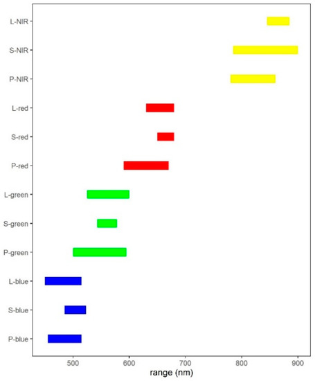
Figure 1.
Bandwidth of satellite image bands. L: Landsat-8, P: PlanetScope, S: Sentinel-2, NIR: near-infrared.
2.2. Study Area
The study area was a 25 × 25 km area in the surroundings of the town of Tokaj, NE-Hungary. The main purpose was to examine an area where as many CLC categories are present as possible. This area contained 19 level 3 categories out of the possible 44. Thus, the area represented a heterogeneous landscape mosaic concerning the landscape elements (i.e., patches), as it is located at the junction of five different microregions with various land types of different characteristics, including floodplains along the Tisza and Bodrog rivers, the hilly areas of the Tokaj hill in the center of the study area, and the sandy plains in the southeast part of the study area [40]. We aggregated the categories in the area into 5 main categories according to the CLC level 1 nomenclature [27] (Figure 2).
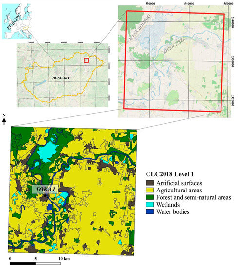
Figure 2.
Study area location and Corine Land Cover level 1 (CLC L1) categories.
2.3. Image Processing
The workflow started with the tasks related to GIS processing: reprojection of the CLC2018 vector dataset from the ETRS89 to the UTM34N coordinate system and clipping to match the study area extent. Then we extracted the descriptive statistical values (minimum, mean, median, maximum, standard deviation (STD)) of the pixels of each satellite band (blue, green, red (RGB), near-infrared (NIR) bands and the calculated NDVI layers) covered by CLC polygons. This resulted in 15 variables (3 sensors × 5 layers). This part of the workflow was performed in QGIS 3.10 [41].
2.4. Statistical Analysis
The extracted dataset was processed with R software [42] using “ggplot2” [43] and “multcomp” [44] packages. Distributions of the variables were tested for normality with the Shapiro–Wilk test. We applied the -2-way ANOVA test based on 20% trimmed values to test the median of the reflectance values (dependent variable) against two independent variables. In addition to nominal factors (the independent variables: CLC categories, satellites), we also included the analysis of interactions to reveal if a factor is influenced in the function by another factor [45]. Satellites had different spatial resolutions; thus, in increasing order, it was suitable for the main effect and the abscissa of the interaction plot, while the land cover categories formed the other main effect.
We applied General Linear Modeling (GLM) to determine the most important biasing factors of the reflectance values. Independence of data was ensured by using the aggregated values (i.e., mean and STD) of the CLC polygons, variance homogeneity was checked by the Levene test, and the normal distribution was checked by the Shapiro–Wilk test. We performed two GLMs; in the first model, the median of the reflectance was the dependent variable, while in the second model, the STD, the independent variables were the following factors: land cover category (L1), the satellite type (SAT) and the band of the satellites (band). We also determined the effect size (ω2) to estimate the contribution of the given factors to the variance of the dependent variable [46]; the effect can be categorized as small (ω2: 0.01–0.06), medium (ω2: 0.06–0.14), or large (ω2 > 0.14) [45]. Thus, we were able to evaluate the significance and contribution of the given influencing factors and the statistical interactions. GLMs were conducted in jamovi 1.2.16 [47].
We conducted classifications to reveal whether the CLC L1 level classes can be discriminated by the spectral values of satellite bands and the NDVI. We applied a traditional and parametric method, the Linear Discriminant Analysis (LDA), and a robust nonparametric classifier, the Random Forest (RF).
LDA is a popular method in multivariate statistical analysis and is powerful but has several assumptions. It requires a balanced set of cases within different categories and multivariate normal distribution [48,49,50]. Accordingly, if there are outlier data within the categories, the number of misclassifications will increase. The RF algorithm works with hundreds of classification decision trees: the dataset is sampled as many times as the number of decision trees with bootstrapping (i.e., the same data can be used in the same dataset several times). The number of variables is the square root of the total number of variables. As a consequence of the procedure, there are no limitations or prerequisites; moreover, the approach is efficient [48,51].
We performed the classifications involving all variables, and we then repeated all classifications with the most important variables determined by the Recursive Feature Elimination (RFE). Fewer variables can result in good accuracy and help to avoid overfitting. The RFE works as follows: we need to specify an algorithm (e.g., LDA or RF), and the RFE performs a classification; next, the classification runs again, omitting one variable and recording the validation loss. The variable omission is repeated until all variables are omitted and, based on the contribution of the variables, a rank is produced [52]. The RFE was conducted with the RF algorithm with repeated 5-fold cross-validation with 10 repetitions (i.e., based on 50 models) using the “caret” package of R [53].
2.5. Analysis of Data Representativeness
The representativeness of data is always among the main questions in all studies. Although we had 984 CLC polygons, the water body category had only 39 cases. We aimed to reach 85% accuracy (OA) with 5% allowable error, which requires at least 200 cases according to Foody [54] (Equation (1)), practically 50 cases per CLC-class. We aimed to use a balanced design with the same data size, so we omitted the water category from this analysis. Accordingly, we performed an analysis using stratified random sampling (10 random datasets) and 2-fold cross-validation with 25 repetitions for all random samples; therefore, all randomizations were based on 50 models:
where n is the required number of data, z is the standard error associated with the chosen level of confidence, P is the planned value of accuracy (%), and h is the allowable error (%). In our test z was 1.96 (95% confidence), P was 85%, and h was 5%.
We applied only the RF classifier, including all variables, and applied complete random models (samples came from random sampling, and the RF models were also randomized, as R makes it possible to ensure similar or different model runs). The models’ OA values were evaluated by satellites using ANOVA. Our H0 was that the means of different RF models based on random samples were equal. The Tukey-test was used in the post hoc analysis. We supposed that if the model means were equal, data representativeness is ensured, as reflected in the 10 randomized models; therefore, the results can be general and be true for other areas as well.
2.6. Accuracy Assessment
Classification accuracy was tested with two methods. Overall Accuracy (OA) was tested with a repeated 5-fold cross-validation with 10 repetitions (RCV) [55]. Here, we had split the whole dataset into five subsets and used 4 of them as train data and 1 as a test set; then, another subset was used as the test set and the rest 4 as a train. The process was concluded when all subsets were used as a test set, and the whole procedure was repeated 10 times. Finally, we obtained 50 models, and we could calculate the medians, quartiles, minimums, and maximums of OAs for each model. Classification accuracy on the category level was evaluated using the traditional approach of Congalton [13], based on the confusion matrices and the derived accuracy metrics: User’s Accuracy (UA) and Producer’s Accuracy (PA). We used the 10 randomizations of data representativeness to determine the ranges of UA and PA (instead of reporting only one confusion matrix). Classification accuracy was determined with the “caret” package of R [53].
3. Results
3.1. Differences of Spectral Characteristics of CLC Categories
The spectral bands of different satellites had significant differences (p < 0.05 according to Tukey’s test), i.e., CLC polygons of the same category were represented by different statistical parameters.
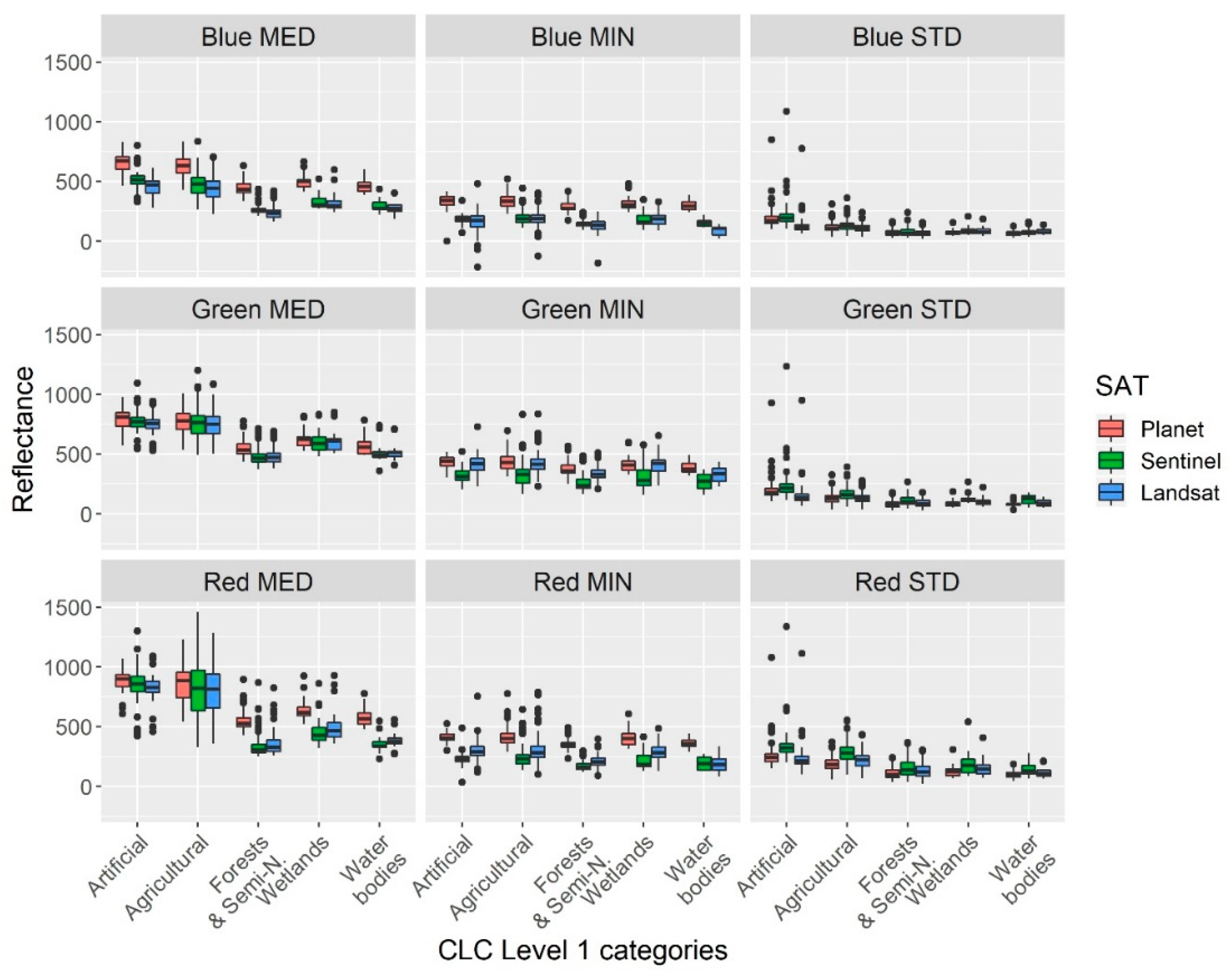
Regarding the visual bands, the median and minimum of the blue and the minimum of the red bands in the PlanetScope image had significantly higher (p < 0.05) values compared to the other two sensors. In either blue, green or red median graphs, artificial and agricultural categories showed significantly higher values with all sensors than the forest, wetland and water bodies categories. STDs were significantly higher (p < 0.05) in the case of Sentinel-2 data for almost all categories in RGB bands (Figure 3).
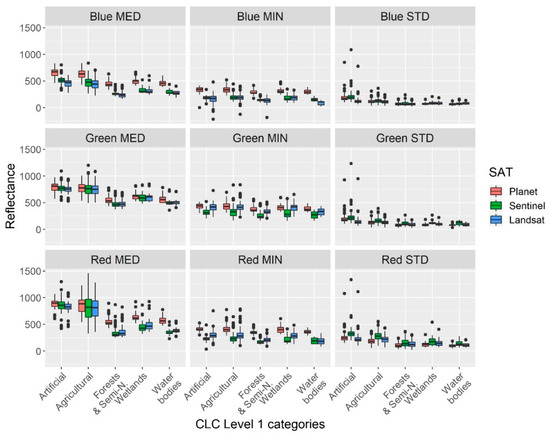
Figure 3.
Distribution of the blue, green and red band pixel values of each sensor for the median (MED), minimum (MIN) and standard deviation values (STD) in each Corine Land Cover (CLC) polygon of CLC level 1 categories (median, quartiles, outliers).
3.2. Reflectance Values and Nominal Factors
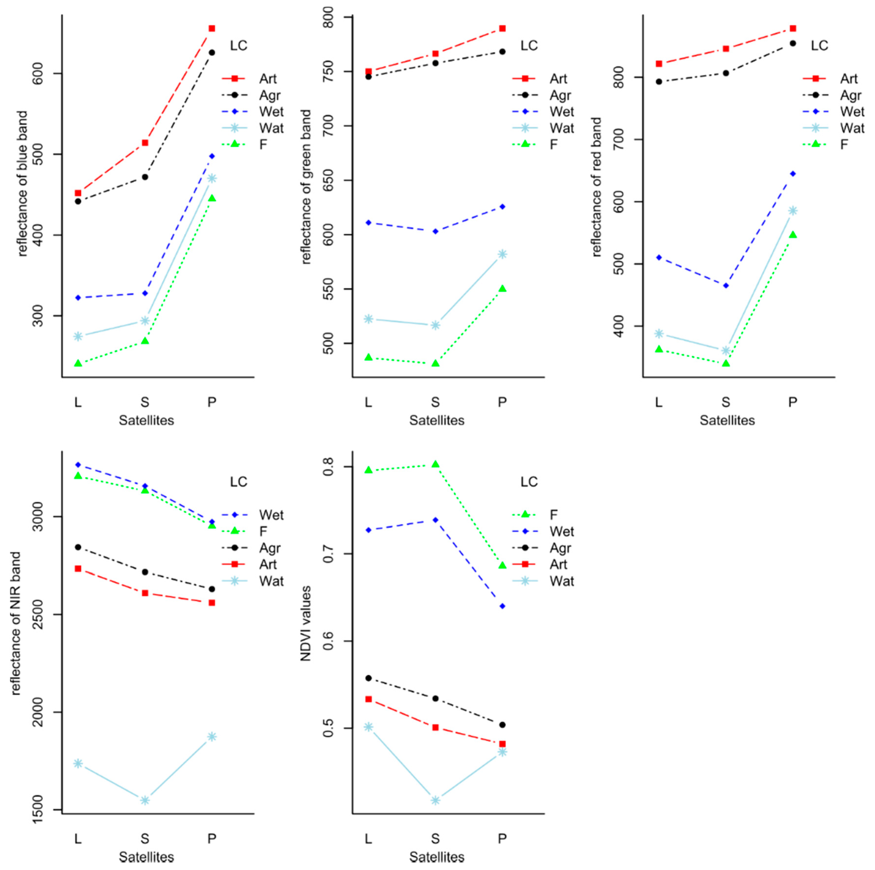
The 2-way ANOVA revealed that both satellite type (SAT) and land cover category (L1) had significant effects in all cases. Furthermore, there was a significant interaction effect in the case of red, NIR bands and NDVI, i.e., CLC categories were affected by the satellite sensors differently in these cases (Table 1; Figure 4). Regarding the visible bands, the agricultural and artificial areas and the water, wetland and forest categories formed groups. In the case of the NIR band, the groups were almost the same, but the highest values were found in the forests and wetlands, and water was placed at the bottom of the diagram (Figure 4). Regarding the NDVI, agricultural, artificial and water categories were in one group with lower values and forests and wetlands in another group with higher values.

Table 1.
Differences between the reflectance values regarding the satellites (SAT) and Corine Land Cover (CLC) categories (L1) and their statistical interaction (SAT: L1) based on the two-way factorial ANOVA. NIR: near-infrared, NDVI: Normalized Difference Vegetation Index.
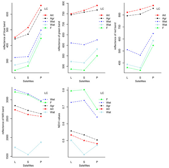
Figure 4.
Interaction plot of reflectance values by satellites and Corine Land Cover (CLC) categories. L: Landsat, S: Sentinel, P: PlanetScope; LC: land cover, Art: artificial, Agr: agricultural, F: forest, Wet: wetland, Wat: water, NIR: near-infrared, NDVI: Normalized Difference Vegetation Index.
GLMs revealed that the variance of reflectance values’ medians and STDs could be explained by the independent factors involved. When medians were the dependent variable (Table 2), the adjusted R2 was 0.972, and all factors and their interactions were significant (p < 0.001). Satellite bands made the largest contribution to the explained variance; the next largest was the interaction of the bands and land cover classes (L1), and the L1 alone also made a small contribution. The model with the STD as the dependent variable was also strong; the adjusted R2 was 0.895 (Table 3). Regarding the contributions, similarly to medians, satellite bands had the largest effect, and the interaction of bands and LCs (band × L1) and the LCs alone (L1) was also in the second and third place. However, in this case, the satellite type (SAT) and its interaction with the bands (SAT × bands) had a small effect.

Table 2.
Summary of General Linear Model (GLM) performed with medians calculated from CLC polygons. SS: sum of squares, df: degrees of freedom, F: F-statistic, p: significance, ω2: effect size; L1: land cover class; SAT: satellite type; band: satellite bands.

Table 3.
Summary of General Linear Model (GLM) performed with standard deviations calculated from CLC polygons. SS: sum of squares, df: degrees of freedom, F: F-statistic, p: significance, ω2: effect size; L1: land cover class; SAT: satellite type; band: satellite bands.
3.3. CLC Categories as Reflected in Classification Algorithms
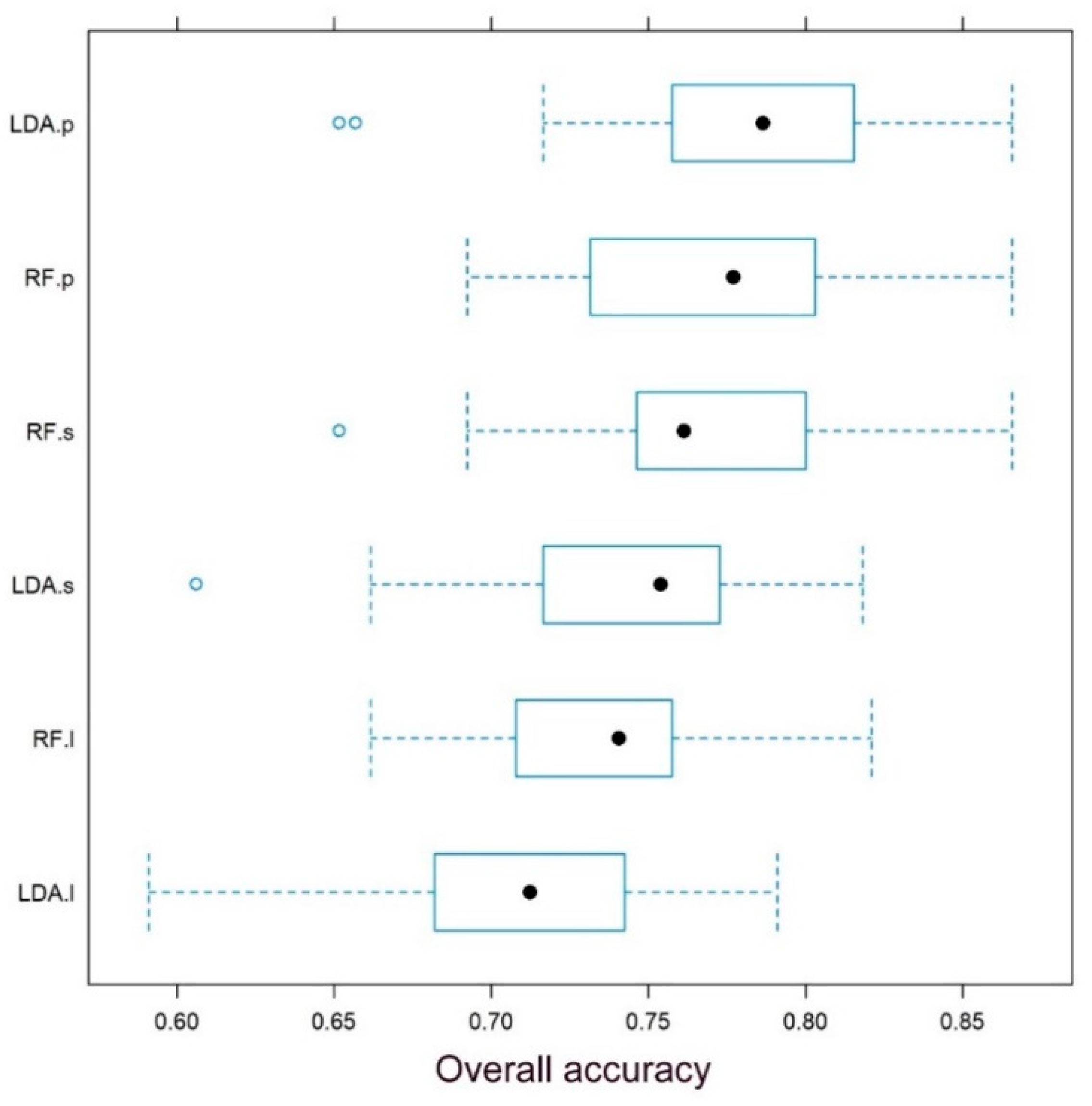
Classifications revealed that the best classification accuracies (OAs) belonged to the PlanetScope satellite, while the Landsat provided the worst; however, the medians of 50 models (for each algorithm and satellite data from the 10-fold cross-validation with 5 repetitions) ranged between 71.1% (LDA with Landsat data) and 78.5% (LDA with PlanetScope data; Figure 5). Although LDA provided the best median of OAs, RF was only 1% worse; furthermore, the median was only one parameter: the minimum value was 65.1% for LDA, and 69.2% for RF and the maximums were equal (86.5%). In the case of Sentinel, the medians of OAs were almost equal: 75.3% (LDA) and 76.1% (RF), but the RF’s minimum and maximum were both higher than the same parameters of LDA. Classification with Landsat data showed the worst performance, and this was especially true of the LDA models where the maximum (79.1%) was worse than the upper quartile of RF.s, LDA.p and RF.p (Figure 5).
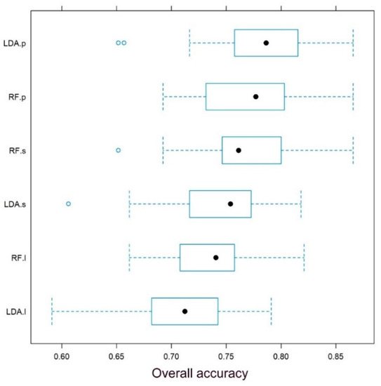
Figure 5.
Overall accuracies by satellites and classification algorithms. LDA: Linear Discriminant Analysis, RF: Random Forest, p: PlanetScope, s: Sentinel-2, l: Landsat-8.
We repeated the analysis with all available bands in the case of Landsat-8 and Sentinel-2, and the OAs improved by 3–6%. We observed the largest (6%) increase of medians in the case of Sentinel-2 classified with LDA, but for Landsat-8, the increase was only 2% (Table 4).

Table 4.
Overall classification accuracies of the common bands (RGB + NIR) and all available bands using all statistical layers. LDA: Linear Discriminant Analysis, RF: Random Forest; l: Landsat-8, s: Sentinel-2; LQ: lower quartile, UQ: upper quartile; RGB: bands of the visible range, NIR: near infra-red.
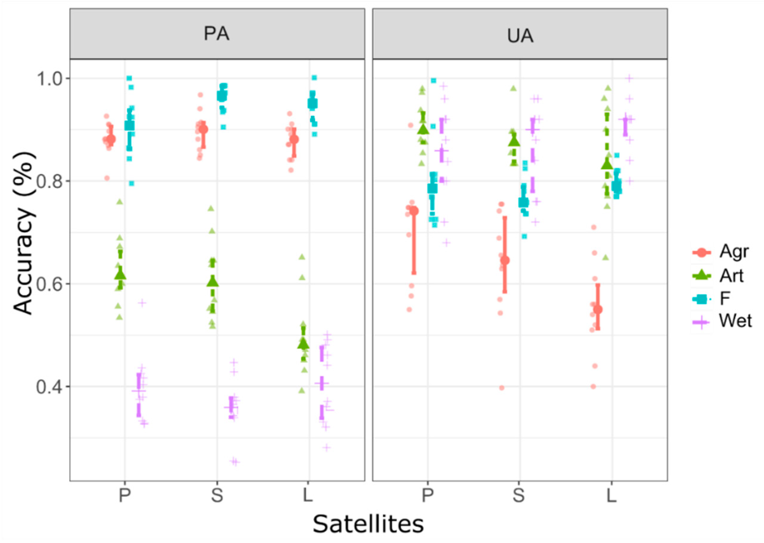
Class level accuracy measures revealed a heterogeneous result (Figure 6). PAs indicated greater accuracies (~90%) for agricultural areas and forests; artificial areas had moderate accuracies (about 60%), while the performance of wetlands was the poorest (even below 40%). Usually, PAs were similar regarding the satellites; the only divergent case occurred in the artificial areas where the models running with Landsat data had the lowest values. UAs were larger than PAs even in the case of the poorest results, which belonged to the agricultural areas (75–55%). Artificial areas and wetlands had the highest values (about 90%), and forest UAs were around 80%. Regarding the satellites, agricultural areas and wetlands had decreasing accuracy as they moved towards coarser spatial resolution (i.e., from the PlanetScope to Landsat). Two-way ANOVAs where the UA and PA were the dependent and the L1 and satellite type were the independent variables showed that the main effect of L1 was significant (F = 17.105, df = 3, p < 0.001), but the main effect of satellites was insignificant (F = 0.642, df = 2, p = 0.527); furthermore, their interaction was also insignificant (F = 0.789, df = 6, p = 0.579).
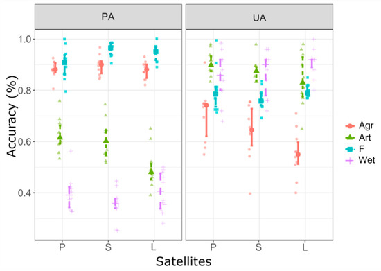
Figure 6.
Median ± quartiles of User’s and Producer’s Accuracies (UA and PA, respectively) of 10 randomized Random Forest classifications. P: PlanetScope, L: Landsat; S: Sentinel; Agr: agricultural areas, Art: artificial areas, F: forest, Wet: wetland.
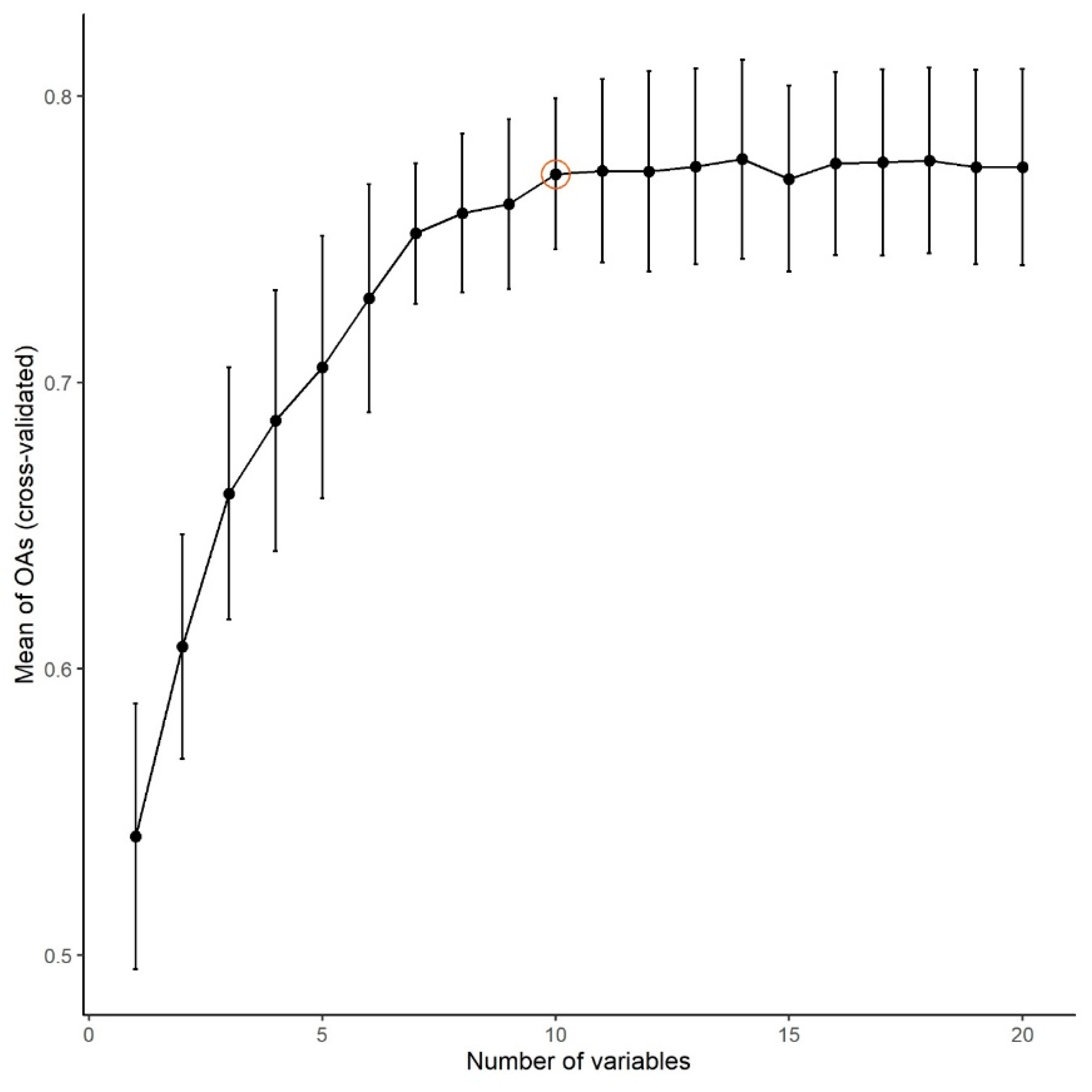
We also investigated the classifications from the perspective of the variables involved. The RFE method revealed that of the 20 available variables (4 bands and the NDVI with minimum, maximum, median and STD), the best performance could be gained with 14 variables (Figure 7). Accordingly, the most important variables in decreasing order were the following: (1) GREEN_med, (2) RED_med, (3) NDVI_med, (4) NIR_med, (5) BLUE_std, (6) NIR_std, (7) BLUE_med, (8) NDVI_std, (9) RED_std, (10) GREEN_std, (11) GREEN_max, (12) BLUE_max, (13) NIR_min and (14) BLUE_min. Besides the means, standard deviations also changed with the number of variables: up to five variables had STDs above 0.045, while for between 7 and 10 variables, it decreased to <0.03; however, after involving more than 10 variables, the SD increased again. Thus, the best outcomes occurred when using the first ten variables.
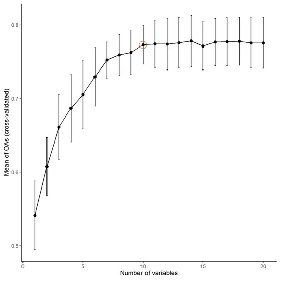
Figure 7.
Means and standard deviations of overall accuracies. 30 models: 10-fold cross-validation with 3 repetitions, the red circle indicates the model with 10 involved variables.
3.4. Data Representativeness
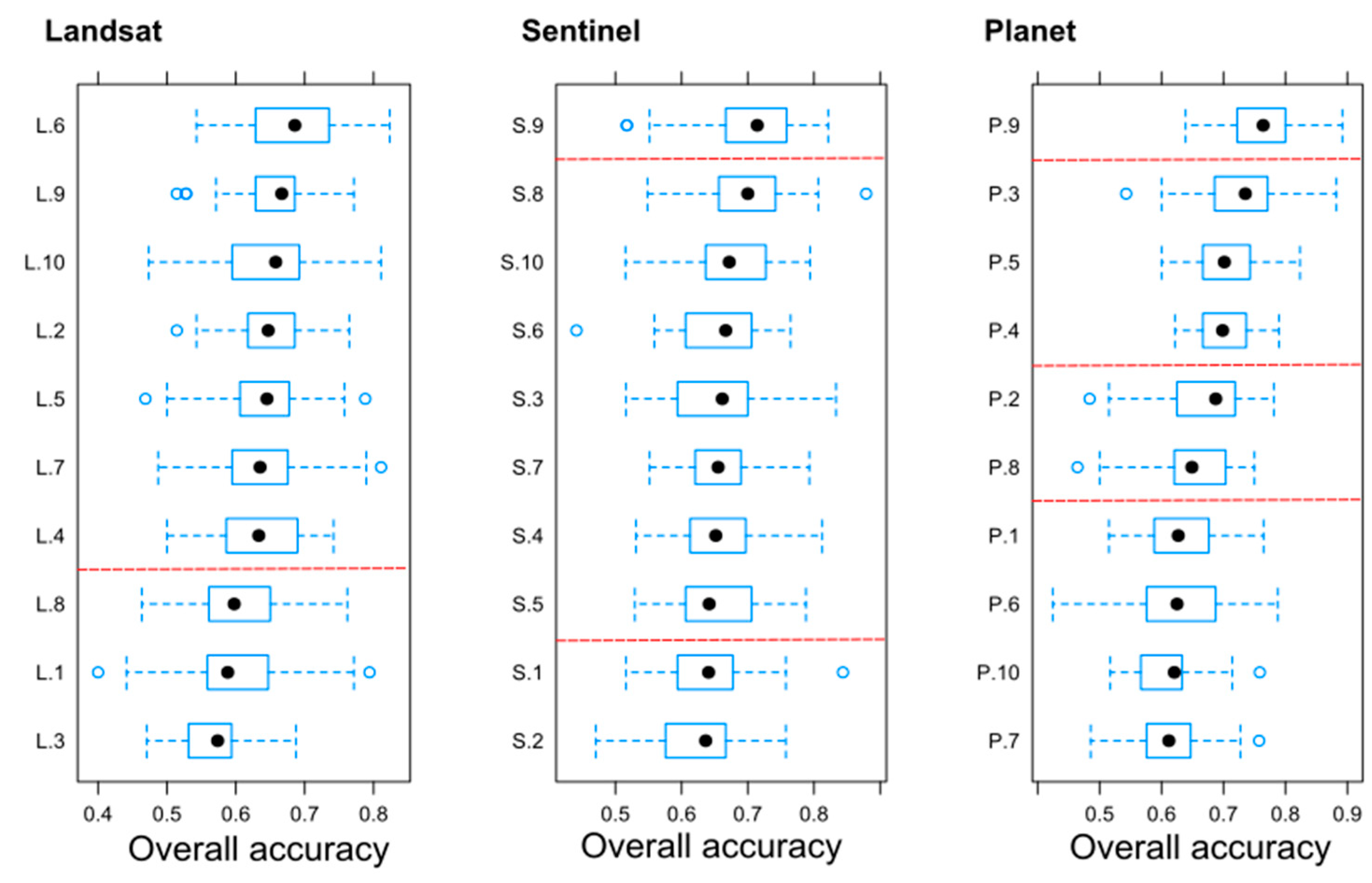
A crucial question is how the data represent the study area. Our randomized sampling, using randomizations combined with 50 classifications per satellite (10 × 50 × 3, 1500 models), showed that results had minor differences (Figure 8). Our hypothesis was that if the OA means of 50 models do not differ significantly by randomizations, the results are representative because input data do not influence classification accuracy. In the case of Landsat and Sentinel satellites, classification accuracies were statistically equal in 7 cases out of the 10 randomizations. Landsat had two groups (7 and 3 randomizations), and the difference between the best and worst OA medians was 10% (L.4 and L.8 according to Figure 8). The difference between the statistically different groups (i.e., the threshold) was 3.3%. Sentinel had 3 groups, and the difference between the poorest and the best performance was 7.8%. Although the difference was significant (p < 0.05) between S.8 and S.9 (according to Figure 8) in statistical terms, the difference between OA medians was only 1.42%; therefore, the effect (the magnitude of differences) was low. Regarding the other threshold (between S.5 and S.1), the difference of medians was only 0.2. In the case of PlanetScope, differences were more enhanced, as the 10 randomizations formed 4 groups. The differences between the best and worst model were the highest among the satellites, reaching 14.4%; however, differences between the two sides of the thresholds were 2.9% (P.9 vs. P.3), 1.1% (P.4 vs. P.2) and 2.2% (P.8 vs. P.1). A change in the minimums regarding P.4 and P.2, from 51.1% to 46.4%, can explain the statistical difference; the remaining groups, however, had theoretical relevance.
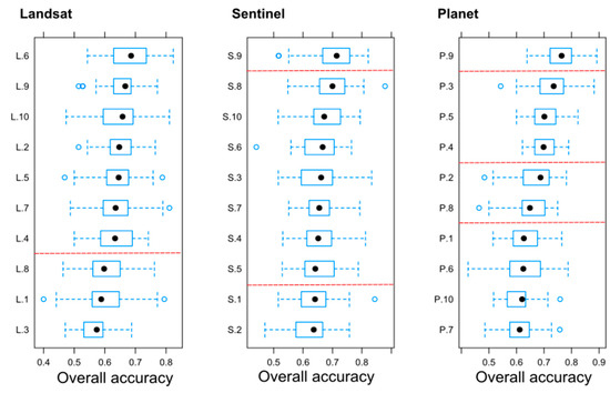
Figure 8.
Overall accuracies of different random samplings by satellites. Boxplot: minimum, lower quartile, median, upper quartile, maximum, blue circle: outliers; red dashed line: the threshold between significantly different groups.
4. Discussion
4.1. CLC Classes and the Mixture of Spectral Features
CLC maps were visually interpreted, and the reported thematic overall accuracy (OA) was ≥85% [56]. However, OA, as a general index, cannot express the errors on the level of categories. Although validation data of photointerpretation is available [57], it is also important to verify whether CLC categories have a direct relation to LC maps derived from satellite images. Although there is only limited information about the class level accuracy on CLC classification, several studies use it as ancillary reference data, e.g., [58,59]. However, other studies used the CLC directly as reference data. Gudmann et al. [19] performed a LULC classification using Sentinel-2 and Landsat-8 images combined with OBIA (object-based image analysis) and the landscape metric approach [60] and found good correspondence. Their study relied on the accuracy assessment with the CLC2018; thus, this research had the most similarity to our work. The OAs of the two study areas were higher in a homogenous area (91%) and almost the same (76%) in the case of the complex one. Although their approach was exactly the inverse of our research question (i.e., they classified images and used the CLC as a reference, while we intended to justify classes of CLC polygons using the reflectance values of satellites), the final result of the classification was almost the same in case of the complex area having the most similarities with our study area. Reyes et al. [61] also used the CLC maps as reference data, and they gained 85.3% OA with OBIA, combining the image classification with landscape metrics. Ceccarelli et al. [62] reported 87–88% OAs for two areas with segmentation and spectral indices and textural information. OAs of our classifications were almost as good as in these studies, but we used the CLC polygons, which was a relevant difference. Verde et al. [63] elaborated a national-level land cover mapping scheme for ecosystem services. They applied superpixel segmentation and, similarly to our approach, used the RF classifier and their best result was an OA of 79%.
Previous studies did not analyze how well CLC polygons are represented by reflectance values of satellite images as LULC classes; instead, pixel or segmentation-based classification was performed on the images. Although these studies had valuable results, their approach was only similar to ours: segments are based on pixel similarity [64], the variance inside the segments is minimal related to the neighboring segments, while CLC polygons are not segments but products of a visual interpretation. Thus, while segments represent homogenous pixel groups [64] (can be regarded as raw data), CLC polygons show real information about the delineated areas.
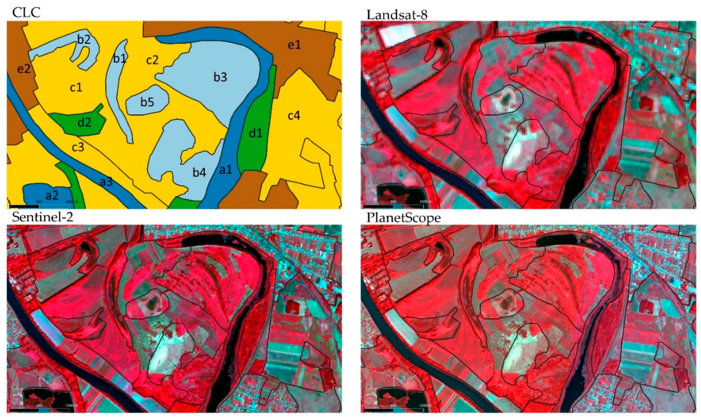
The CLC Technical Report [57] confirmed that 78% of all classification errors occurred on Level 2 and 3 nomenclatures; thus, the most simplified level 1 was the most accurate. The report also stated that most misclassifications occurred between “agricultural” and “forest and semi-natural” categories. However, a comprehensive accuracy assessment for the CLC2018 map is not available yet. OA of CLC2012 was 90.5% in the L2 and 89.5% in the L3 nomenclature [65]. We demonstrated the issues identified in a smaller part of the study area (Figure 9) in detail. Water bodies (rivers and lakes) are delineated without aiming to find the edges, i.e., trees on the shorelines are also included in the patches. In our example, an oxbow lake (Figure 9/a1) was shown where the aquatic vegetation cover was relevant due to the eutrophic state of the lake [66], and the PlanetScope image was the most efficient to show it. Aquatic vegetation with the surrounding trees can relevantly bias the statistical parameters of this polygon of the “water” class, which can be observed both in the case of a fishpond (Figure 9/a2) and the Tisza River (Figure 9/a3). The wetland areas #b1 and #b2 in Figure 9 were also oxbow lakes, but in the next phase of the succession, the proportion of open water was lower, and according to the CLC classification, these lakes were interpreted as wetlands (as these smaller lakes can run dry during dry summers [67], the classification can be accepted). The wetland area #b3 (Figure 9) was a set of swales and point bars (i.e., negative and positive fluvial forms) with different water cover and height of vegetation, where the reflectance pattern can be similar both to grasslands and eutrophic lakes [68,69]. The wetland area #b4 (Figure 9) was also a set of swales and point bars (consisting of two different parts, of which the northern part was the older with transformed forms), while the fifth wetland area (Figure 9/b5) was a floodplain lake with its surroundings (open water with aquatic vegetation and marshlands). This means that there were five wetlands, with four types of appearance, i.e., with different patterns, and suffering from varying errors regarding the right patch contours. In addition, the agricultural areas were mostly pastures within the floodplain (Figure 9/c1–2), but the #c2 patch, for example (in the triangle formed by #b1-#b3-#b5, Figure 9), was also a set of swale-point bar series with lesser water cover related to wetlands #b1, #b2 or #b3, with water patches and mixed with bushes and trees. In dry summers, all wetlands run dry; thus, when this happens, the difference between these pastures and wetlands is small. While #c1 and #c2 were grasslands (coded as 231 in CLC), #c3 and #c4 were intensive agricultural areas (coded as 211 according to the CLC nomenclature), with different spectral features with bare soil among the plants (or even harvested in August), but also consisting of dense plant cultures. Even the forests were different: #d1 was a semi-natural floodplain forest, the patch of #d2 was a plantation with regular rows and smaller density. Settlement patches also represented varying land cover, while #e1 (Figure 9) was a village (Rakamaz), #e2 was only a resort area with some summer houses and many trees and grassland areas. These issues arose from the fact that CLC in some cases is a land-use map rather than a land cover one; the MMU of 25 ha is also a limitation, and the aim of the mapping is to provide a consistent map of a whole country (and finally of the EU). Accordingly, we cannot state that the CLC-interpretations were wrong but merely different from a satellite-based land cover classification. LC classes can be mixed without the problem of the CLC polygons due to similar pixel values and patterns, but these identified issues can help to understand the mixture of reflectance values of the CLC classes: differences are not significant, and the classifications never reach 85%.

Figure 9.
Land cover classes of the Corine Land Cover (CLC) database and their appearance in pseudo-color (near-infrared-red-green) satellite image composites in a smaller part of the study area. a: water, b: wetland, c: agricultural areas, d: forests, e: settlements.
The visually interpreted polygons cover different surfaces, and as the MMU is 25 ha, there are patches smaller than the MMU, and these should be merged into larger patches. That was the case with the smaller oxbow lakes along the Tisza and Bodrog Rivers: instead of water bodies, the lakes were categorized as wetlands with their surroundings. Furthermore, interpretation of CLC classes does not require an accurate delineation, and pixels at the edge of neighboring patches can be mixed. The best examples were the rivers and lakes: aquatic vegetation and floodplain forests were mixed into the water category, and this caused higher maximums in the case of the NIR band and NDVI. According to the CLC2018 validation documentation, the overall thematic accuracy is above 85%, and spatial accuracy is better than 100 m for the whole dataset [56], but regarding the category-level thematic accuracies, the only available documents refer to other European countries, not Hungary (e.g., Finland: [70]). A possible 100 m shift could cause serious errors with satellite images even with a 30 m spatial resolution related to reference land cover, but our visual analysis showed a very good fit among the CLC and the images; inaccurate patch contours had a larger bias in the analysis.
NDVI layers experienced much less category mixture in the case of minimum, standard deviation and maximum values. Due to the fact that the NDVI is a widely-used robust index for distinguishing main land cover classes [71,72,73,74], it may have become helpful in separating the main CLC categories. Miomir et al. [75] investigated opportunities for a good practice of updating the national forest inventory in Serbia by comparing CLC and NDVI-based solutions based on Landsat images from different years. They performed comparisons both with CLC forest areas (based on various CLC categories) and forest areas derived from NDVI maps to official statistical forest data, where they identified a much larger difference in the case of CLC products. Diaz-Pacheco and Gutiérrez (2014) [76] examined the accuracy of CLC products through the analysis of local study areas focusing on urban land cover classes and found that CLC is not appropriate for local studies but rather for global and regional scale analyses. We also found that in our dataset, the artificial class showed a mixture in the case of minimum values with all other categories and in the case of median values, characteristically with the agricultural class. In order to make more detailed land cover datasets even using CLC, there are initiatives to produce new variations of land cover databases [77,78]. There are examples of the use of the CLC data solely to perform land change analysis [79], where the real thematic accuracy of the dataset is less important since the changes are derived from the comparison of consecutive CLC datasets.
4.2. CLC Classes in the Light of Statistical Tests
The two-way ANOVA revealed that both the L1 level CLC categories and the satellite types had significant differences. This is important, but the interaction effect is also important because if the two main effects have a common influence, differences in surface reflectance values are determined by both, i.e., in the case of blue and green bands, there is no difference; thus, input data from the satellites do not have an influence on the reflectance values delineated by the CLC categories. However, in the case of red, with the NIR and the NDVI, the interaction effect was significant; thus, the satellite data type can be considered important from the perspective of land cover representation. GLM also pointed to the relevance of bands and interactions with the LCs, but there was a magnitude difference in the contributions. In the case of medians, dependent variable bands had an ω2 of 0.416, while the interaction of bands and LCs was only 0.023. STDs as dependent variables had a similar result, but the ω2 was 0.515 for the bands and 0.009 for LCs, and there was a ω2 of 0.005 for the interaction of satellites and bands. This means that medians are less biased by the satellite types, but STD can point to the differences among the sensors. On one hand, this may be the reason for the details determined by the spatial resolution. Especially on Landsat images, details can disappear, e.g., in the case of the oxbow lake (Figure 9/a1), aquatic vegetation hardly appears, but PlanetScope revealed that there was a relevant amount of floating aquatic vegetation on the water surface. Thus, PlanetScope can show a more realistic picture of the area because of its 3 m resolution. Due to this high spatial resolution, new biasing factors become visible, including the shadows of trees and buildings. On the other hand, the wavelength ranges of the bands also differ according to the satellite. Sentinel-2 has the narrowest band ranges (usually a half or a third compared to PlanetScope), except for the NIR band, where it was almost three times the Landsat’s range. As the NIR range is important to identify vegetation, it can make Sentinel-2 better in finding forest and agricultural areas, which confirms the results of a class level accuracy assessment (Figure 6) with high PA and low UA values. Sentinel-2 data resulted in a lower error of omission and a higher error of commission regarding the vegetation, as under similar circumstances, it collects more photons than other sensors in the NIR range, influencing the outcomes of classifications. However, the effects of spatial resolution and the wavelength ranges cannot be separated with statistical tests: ranges have only 12 combinations (3 satellites × 4 bands), which is equivalent to the results of the 2-way ANOVA test and GLM. Both tests justified the common effect (interaction), but this proves that the bands involved (RGB + NIR) have different effects according to satellite, and the effect derives from the different spatial resolution and the band reflectance values, which also vary by the wavelength ranges.
4.3. CLC Classes and Classification Algorithms
Based on the classifications, the OAs reflected the fact that ~70% accuracy can be reached using five level 1 CLC categories. LDA as a classifier with several presumed prerequisites did not perform relevantly worse than the robust RF, at least regarding the same satellite data: differences were even below 3% in the worst case (Landsat) for all descriptive statistics except for the minimum (LDA’s minimum was 7% worse than RF’s). Furthermore, LDA, although it did not have all prerequisites ensured, outperformed the RF in the case of PlanetScope data’s classification. We experienced several cases in which LDA’s performance was high in the OA level, but on a class level, it was not so effective [48,51], and the error of commission was especially high. Moreover, LDA had a worse performance with Sentinel and Landsat data, and it reflected the general observations that RF performs well with any kind of training data [80,81,82]. The repeated k-fold cross-validation was a powerful tool to assess classification efficiency, as 30–50 models can provide enough data to have a distribution of the outcomes and to determine the range of outcomes’ accuracy. In our case, the numerous models indicated that in the case of LDA, the worst models could perform with an OA of at least 59.1%, while in the case of RF, the lowest accuracy was 65.1%. This 6% difference can be important; therefore, we suggest using the robust RF for this kind of classification.
Better OAs belonged to higher geometric resolution: 71.1% was the median OA for Landsat and 78.5% for the PlanetScope when we applied the overlapping spectral bands. However, both Landsat-8 and Sentinel-2 have more bands in the infra-red range, and involving these bands into the classification, OAs increased, and Sentinel-2 overperformed the best OA of PlanetScope, i.e., better spectral resolution helped to overcome the disadvantage of coarser geometric resolution. Szabó et al. [82] and Underwood et al. [83] also came to a conclusion to the importance of spectral information, but with the remark of aims of given studies and the involved images (i.e., both hyperspectral and Landsat-8 images can provide eligible outcomes for given purposes, but a very high-resolution hyperspectral image is always a better input for specified tasks).
Randomized sampling from the whole dataset resulted in worse classifications; minimum OAs were between 40 and 44%, medians between 60 and 66% and maximums between 82 and 89%. However, the rank changed compared to the previous results when all data had been used for the classifications: PlanetScope data provided the lowest accuracies, and the Landsat, with coarser spatial resolution, had the best results. The difference between the results was the number of cases in the input data; the omission of the water category could also have an effect on the accuracies and the fact that only 50 data were used per category to train the models. Water body is a usually well distinguishable land cover class [84,85,86], but due to the low number of cases, we excluded it from the analysis, which could reduce the OA by having fewer true positive polygons. The other possible reason is that the different spatial resolutions could also have a bias through the number of pixels involved in a given CLC-category: statistical parameters were calculated by polygons with 9 times more data with the Sentinel and with 100 times more with the PlanetScope satellites compared to Landsat. As previous studies found that finer resolutions should contain spectrally clearer pixels, which have a lesser influence on heterogeneous areas [1,87,88], we can suppose a considerable effect for the missing water category and the lower number of training polygons.
UA and PA values can provide further clues, highlighting that there were large commission errors in the case of agricultural areas and large omission errors in wetlands and artificial areas, which corresponded to the statistical analysis of spectral bands (Section 3.1). Both types of errors can be understood when we are aware of the advantages of visual interpretation: interpreting personnel can make decisions based on several other options than the spectral features, such as the extent/size, relative situation, texture, and pattern of a given object. In this study, we were able to involve only the spectral characteristics, and the classifications were within an acceptable range. There can be relevant intermixing among agricultural areas, grasslands, and forests, and even with wetlands in special situations [36]. Furthermore, artificial surfaces contain built-in areas (buildings, roads, pavements, parking lots), parks (relating to forests or grasslands) and even water features (fountains and lakes, sometimes streams, rivers), so this category can intermix with several natural categories, too. Spectral features are naturally similar in these spectral ranges; thus, we cannot expect clear discrimination. In this study, we supposed that better resolution provides better classifications, but it was true only in the case of OAs; according to the two-way ANOVA conducted on the UA and PA, the satellite type (i.e., the spatial resolution and the different wavelength ranges of the bands) had no influence on the class level accuracy measures of the final products. This finding can only be explained by the visual interpretations and limitation of the MMU size.
Regarding the variables, RFE with the repeated k-fold cross-validation effectively pointed to the relevance of medians (the first four variables in the models) and that green and red bands were more important than NIR and NDVI. Similarly, Chiang and Valdez (2019) [89] also found that green and red bands of Landsat-8 were important in identifying tree species. However, Puletti et al. [90] found that blue and green bands of higher wavelengths, red-edge and NIR, were the most important in the classification of Mediterranean forests. The source of the differences may be that we applied a method, which can be regarded as a special segmentation approach with a different statistical-based technique; furthermore, Puletti et al. [90] applied several dates to gain the best accuracy, while in our study, we used only one. Grabska et al. [91] also found that red-edge, blue and green bands were among the first four most relevant variables. Both studies dealt with forests, and in our case, a further reason for the difference can be found in the categories: artificial areas, agricultural areas, wetlands, water bodies require different sets of involved bands. Sentinel performed 3–6% better when involving all possible bands (red edge and middle-infrared), but in the case of Landsat, the increase of OAs was only 1–2%.
A final major question is how the results can be generalized. Our randomization with 10 randomized sub-samplings showed that not all classifications were similar. The ANOVA model using Tukey’s test as a post hoc test revealed that 3 of the 10 models were different in both Landsat and Sentinel, which may be the basis for concluding a possible generalization. Although statistical tests can find significant differences, the magnitude of the differences may be small (i.e., the differences are not relevant; [92]). Furthermore, Tukey’s test is more liberal (i.e., it finds more statistical differences than other post hoc tests [93]). In this study, median differences between the groups of accuracies were only 1–2%; thus, statistics did not show a real picture. In the case of PlanetScope, models can be divided into four groups; nevertheless, with no great differences in the OAs, two groups can be distinguished with a relatively larger (4%) difference. Thus, the results suggest that PlanetScope’s reflectance values can provide different accuracies when different training datasets are used; CLC polygons and the generalization were not as successful as in the case of Landsat’s and Sentinel’s data.
Validation of remotely sensed data using CLC datasets as a reference may be a misleading step due to the conclusions drawn in contemporary literature concerning the usage recommendations for the data. Our results revealed that the main categories of CLC could not have been discriminated spectrally from each other in satellite images. However, by paying attention to the descriptive statistics, it is possible to involve this information in a classification that takes pixel statistics into consideration [94,95], and it may provide helpful information to know the mixture of categories in the image we intend to use as an input for the classification. Accordingly, it is critical to know the possible mixing behavior of the categories in order to achieve a successful classification.
5. Conclusions
We analyzed the polygons of the CLC2018 database with respect to pixel information derived from PlanetScope, Sentinel-2 and Landsat-8 images. We calculated median, minimum, maximum and standard deviation for all polygons of the CLC2018 concerning the visible and near-infrared bands and a calculated NDVI layer for the three satellites.
- -
- Medians of CLC polygons provided the least mixture among the LC classes, while the maximums were the worst input parameters without significant differences. Wetlands and water bodies categories were the most frequently mixing categories of CLC based on reflectance values;
- -
- Bivariate statistical tests cannot provide enough information to conclude on the spectral separability of LC classes, but classification algorithms involving several variables can be efficient techniques. Generally, LDA and RF classifiers had similar OAs, but in the case of coarser resolutions (Sentinel and Landsat), RF outperformed the LDA. Data derived from PlanetScope provided 7% better OAs (78%) than those of Landsat (71%) regarding the model medians; thus, better spatial resolution ensured better classification performance. >80% OA was gained with using all available bands of the Sentinel-2; accordingly, more spectral information in the infra-red range can counterbalance the coarser geometric resolution;
- -
- We applied a randomization-based technique to gain 10 repetitions of class-level metrics (UA and PA), which showed that satellites had no direct effect on the accuracy. UAs were the lowest in agricultural areas, while PAs were the lowest among wetlands;
- -
- Variable importance of statistical parameters showed that usually the medians were the most important statistical layers, and the green, red and near-infrared bands were the first three most important bands;
- -
- We provided an approach to prove the possibility of the generalization of the results with multiple randomized subsampling and found that the results of Landsat and Sentinel data can be generalized, but in the case of PlanetScope, a larger area with more CLC polygons would be desirable;
- -
- Generally, using the overlapping bands (RGB + NIR) of Landsat-8, Sentinel-2 with the PlanetScope, the best OAs were >70% OAs, but the most accurate was the PlanetScope with the highest spatial resolution (78.5%). Higher OAs (~80%) have also been acquired with the higher spectral accuracy of the Sentinel-2, which means a cost-efficient solution in spite of the coarser spatial resolution;
- -
- As we found several studies where CLC maps were used as ground truth data to quantify thematic accuracy, 70–80% OAs do not seem satisfactory. Nevertheless, our experiment was performed with the CLC L1 classes; further investigations can reveal if CLC is more appropriate for ground truth with the more detailed L2 or L3 nomenclature.
CLC maps have many features limiting their use as validation data. The 25 ha MMU size creates several issues, which influence validation by satellite images: land cover polygons do not follow the exact borders of patches, smaller objects are merged into larger ones to reach the 25 ha area, and even the supposedly homogenous patches also have a nonhomogeneous texture (e.g., lakes, rivers).
Author Contributions
Conceptualization, O.G.V. and S.S.; methodology, O.G.V. and S.S.; validation, O.G.V. and S.S.; formal analysis, O.G.V., Z.C.S., S.S. and Z.K.; investigation, O.G.V. and S.S.; resources, O.G.V. and I.H.; data curation, O.G.V., S.S., S.N., L.B. and Z.K.; writing—original draft preparation, O.G.V., S.S., P.B., L.B., Z.C.S. and S.N.; writing—review and editing, O.G.V. and S.S.; visualization, O.G.V., Z.K., Z.C.S. and S.S.; supervision, S.S.; project administration, L.B. and P.B.; funding acquisition, S.S., I.H. and O.G.V. All authors have read and agreed to the published version of the manuscript.
Funding
On behalf of O.G.V., the research was supported by the ÚNKP-19-3-III-DE-94 New National Excellence Program of the Ministry for Innovation and Technology. The research was supported by the TNN 123457 NKFI and the Thematic Excellence Programme (TKP2020-NKA-04) of the Ministry for Innovation and Technology in Hungary projects.
Data Availability Statement
Calculated data is available on request. CLC map and the Landsat-8 and Sentinel-2 satellite images are available for download at public repositories. The Planet images are the property of Planet Lab.
Conflicts of Interest
The authors declare no conflict of interest.
References
- Deák, M.; Telbisz, T.; Árvai, M.; Mari, L.; Horváth, F.; Kohán, B. Heterogeneous Forest Classification by Creating Mixed Vegetation Classes using EO-1 Hyperion. Int. J. Remote Sens. 2017, 38, 5215–5231. [Google Scholar] [CrossRef]
- Kishor, B.; Singh, S.K. Change Detection Mapping of Land use Land Cover using Multidate Satellite Data (A Case Study of Pichavaram Mangrove). Int. J. Eng. Res. Technol. 2014, 3, 2320–2326. [Google Scholar]
- Sohl, T.L.; Sleeter, B.M. Role of Remote Sensing for Land-Use and Land- Cover Change Modelling. In Remote Sensing and Land Cover: Principles and Applications; Giri, C., Ed.; CRC Press: Boca Raton, FL, USA, 2012; pp. 225–239. [Google Scholar]
- Bey, A.; Sánchez-Paus Díaz, A.; Maniatis, D.; Marchi, G.; Mollicone, D.; Ricci, S.; Bastin, J.; Moore, R.; Federici, S.; Rezende, M.; et al. Collect Earth: Land use and Land Cover Assessment through Augmented Visual Interpretation. Remote Sens. 2016, 8, 807. [Google Scholar] [CrossRef]
- Burai, P.; Deák, B.; Valkó, O.; Tomor, T. Classification of Herbaceous Vegetation using Airborne Hyperspectral Imagery. Remote Sens. 2015, 7, 2046–2066. [Google Scholar] [CrossRef]
- Li, X.; Chen, W.; Cheng, X.; Wang, L. A Comparison of Machine Learning Algorithms for Mapping of Complex Surface-Mined and Agricultural Landscapes using ZiYuan-3 Stereo Satellite Imagery. Remote Sens. 2016, 8, 514. [Google Scholar] [CrossRef]
- Wessel, M.; Brandmeier, M.; Tiede, D. Evaluation of Different Machine Learning Algorithms for Scalable Classification of Tree Types and Tree Species Based on Sentinel-2 Data. Remote Sens. 2018, 10, 1419. [Google Scholar] [CrossRef]
- Abd El-Kawy, O.R.; Rød, J.K.; Ismail, H.A.; Suliman, A.S. Land use and Land Cover Change Detection in the Western Nile Delta of Egypt using Remote Sensing Data. Appl. Geogr. 2011, 31, 483–494. [Google Scholar] [CrossRef]
- Almeida, C.A.; Coutinho, A.C.; Esquerdo, J.C.D.M.; Adami, M.; Venturieri, A.; Diniz, C.G.; Dessay, N.; Durieux, L.G.; Rodrigues, A. High Spatial Resolution Land use and Land Cover Mapping of the Brazilian Legal Amazon in 2008 using Landsat-5/TM and MODIS Data. Acta Amaz. 2016, 46, 291–302. [Google Scholar] [CrossRef]
- Pinto, A.T.; Gonçalves, J.A.; Beja, P.; Pradinho Honrado, J. From Archived Historical Aerial Imagery to Informative Orthophotos: A Framework for Retrieving the Past in Long-Term Socioecological Research. Remote Sens. 2019, 11, 1388. [Google Scholar] [CrossRef]
- Bielecka, E.; Jenerowicz, A. Intellectual Structure of CORINE Land Cover Research Applications in Web of Science: A Europe-Wide Review. Remote Sens. 2019, 11, 2017. [Google Scholar] [CrossRef]
- Chehdi, K.; Cariou, C. Learning or Assessment of Classification Algorithms Relying on Biased Ground Truth Data: What Interest? J. Appl. Remote Sens. 2019, 13, 034522. [Google Scholar] [CrossRef]
- Congalton, R.G. A Review of Assessing the Accuracy of Classifications of Remotely Sensed Data. Remote Sens. Environ. 1991, 37, 35–46. [Google Scholar] [CrossRef]
- Hay, A.H. Sampling Designs to Test Land-use Map Accuracy. Photogramm. Eng. Remote Sens. 1979, 45, 529–533. [Google Scholar]
- Yague, J.; Garcia, P. Approaching Corine Land Cover Over Castilla and Leon (Central Spain) with a Multitemporal NOAA-AVHRR NDVI MVC Series. In Proceedings of the Second International Workshop on the Analysis of Multi-Temporal Remote Sensing Images; Smits, P.C., Bruzzone, L., Eds.; World Scientific Publishing: Singapore, 2004; pp. 314–321. [Google Scholar]
- De Santa Olalla Mañas, M.; Soria, C.; Ramírez, A. Validation of the CORINE Land Cover Database in a Pilot Zone Under Semi-Arid Conditions in La Mancha (Spain). Cybergeo Eur. J. Geogr. 2003. [Google Scholar] [CrossRef]
- Rujoiu-Mare, M.; Mihai, B. Mapping Land Cover using Remote Sensing Data and GIS Techniques: A Case Study of Prahova Subcarpathians. Procedia Environ. Sci. 2016, 32, 244–255. [Google Scholar] [CrossRef]
- Caetano, M.; Mata, F.; Freire, S. Accuracy assessment of the Portuguese CORINE Land Cover map. In Global Developments in Environmental Earth Observation from Space; Marçal, A., Ed.; Millpress: Rotterdam, The Netherlands, 2006. [Google Scholar]
- Gudmann, A.; Csikós, N.; Szilassi, P.; Mucsi, L. Improvement in Satellite Image-Based Land Cover Classification with Landscape Metrics. Remote Sens. 2020, 12, 3580. [Google Scholar] [CrossRef]
- Stathopoulou, M.I.; Cartalis, C.; Petrakis, M. Integrating Corine Land Cover Data and Landsat TM for Surface Emissivity Definition: Application to the Urban Area of Athens, Greece. Int. J. Remote Sens. 2007, 28, 3291–3304. [Google Scholar] [CrossRef]
- Golenia, M.; Zagajewski, B.; Ochytra, A. Semiautomatic Land Cover Mapping According to the 2nd Level of the CORINE Land Cover Legend. Pol. Cartogr. Rev. 2015, 47, 203–212. [Google Scholar] [CrossRef]
- Dalponte, M.; Marzini, S.; Solano-Correa, Y.T.; Tonon, G.; Vescovo, L.; Gianelle, D. Mapping Forest Windthrows using High Spatial Resolution Multispectral Satellite Images. Int. J. Appl. Earth Obs. Geoinf. 2020, 93, 102206. [Google Scholar] [CrossRef]
- Messina, G.; Peña, J.M.; Vizzari, M.; Modica, G. A Comparison of UAV and Satellites Multispectral Imagery in Monitoring Onion Crop an Application in the ‘Cipolla Rossa Di Tropea’ (Italy). Remote Sens. 2020, 12, 3424. [Google Scholar] [CrossRef]
- Feranec, J.; Soukup, T.; Hazeu, G.; Jaffrain, G. European Landscape Dynamics: CORINE Land Cover Data; CRC Press: Boca Raton, FL, USA, 2016. [Google Scholar]
- Leinenkugel, P.; Deck, R.; Huth, J.; Ottinger, M.; Mack, B. The Potential of Open Geodata for Automated Large-Scale Land use and Land Cover Classification. Remote Sens. 2019, 11, 2249. [Google Scholar] [CrossRef]
- European Environment Agency (EEA). Corine Land Cover Change (CHA) 2012–2018; Version 2020_20u1; European Environment Agency: Copenhagen, Denmark, 2020; Available online: https://land.copernicus.eu/pan-european/corine-land-cover/lcc-2012-2018?tab=download (accessed on 24 February 2021).
- Kosztra, B.; Büttner, G.; Hazeu, G.; Arnold, S. Updated CLC Illustrated Nomenclature Guidelines. European Topic Centre on Urban, Land and Soil Systems. 2019. Available online: https://land.copernicus.eu/user-corner/technical-library/corine-land-cover-nomenclature-guidelines/docs/pdf/CLC2018_Nomenclature_illustrated_guide_20190510.pdf (accessed on 24 February 2021).
- U.S. Geological Survey. Landsat 8 Fact Sheet 2013-3060. 2013. Available online: https://pubs.usgs.gov/fs/2013/3060/pdf/fs2013-3060.pdf (accessed on 24 February 2021).
- European Space Agency. Sentinel-2 User Handbook. 2015. Available online: https://sentinel.esa.int/documents/247904/685211/Sentinel-2_User_Handbook (accessed on 24 February 2021).
- Planet Labs. Planet Imagery Product Specifications. 2019. Available online: https://assets.planet.com/docs/Planet_Combined_Imagery_Product_Specs_letter_screen.pdf (accessed on 24 February 2021).
- The Hungarian Meteorological Service (OMSZ). Daily Weather Forecast for Hungary 2005–2019. Available online: https://www.met.hu/idojaras/aktualis_idojaras/napijelentes_2005-2019/ (accessed on 24 February 2021).
- Rouse, J.W., Jr.; Haas, R.H.; Schell, J.A.; Deering, D.W.; Harlan, J.C. Monitoring the Vernal Advancements and Retrogradation of Natural Vegetation; Final Report; NASA Goddard Space Flight Center: Greenbelt, MD, USA, 1974; pp. 1–137. [Google Scholar]
- Baret, F.; Guyot, G.; Major, D.J. Crop Biomass Evaluation using Radiometric Measurements. Photogrammetria 1989, 43, 241–256. [Google Scholar] [CrossRef]
- Aredehey, G.; Mezgebu, A.; Girma, A. Land-use Land-Cover Classification Analysis of Giba Catchment using Hyper Temporal MODIS NDVI Satellite Images. Int. J. Remote Sens. 2018, 39, 810–821. [Google Scholar] [CrossRef]
- Gulácsi, A.; Kovács, F. Drought Monitoring of Forest Vegetation using MODIS-Based Normalized Difference Drought Index in Hungary. Hung. Geogr. Bull. 2018, 67, 29–42. [Google Scholar] [CrossRef]
- Szabó, S.; Elemér, L.; Kovács, Z.; Püspöki, Z.; Kertész, Á.; Singh, S.K.; Balázs, B. NDVI Dynamics as Reflected in Climatic Variables: Spatial and Temporal Trends—A Case Study of Hungary. GISci. Remote Sens. 2019, 56, 624–644. [Google Scholar] [CrossRef]
- Ma, J.; Zhang, C.; Yun, W.; Lv, Y.; Wanling, C.; Zu, D. The Temporal Analysis of Regional Cultivated Land Productivity with GPP Based on 2000–2018 MODIS Data. Sustainability 2020, 12, 411. [Google Scholar] [CrossRef]
- Olmos-Trujillo, E.; González-Trinidad, J.; Júnez-Ferreira, H.; Pacheco-Guerrero, A.; Bautista-Capetillo, C.; Avila-Sandoval, C.; Galván-Tejada, E. Spatio-Temporal Response of Vegetation Indices to Rainfall and Temperature in A Semiarid Region. Sustainability 2020, 12, 1939. [Google Scholar] [CrossRef]
- Roy, D.P.; Yan, L. Robust Landsat-Based Crop Time Series Modelling. Remote Sens. Environ. 2020, 238, 110810. [Google Scholar] [CrossRef]
- Dövényi, Z. Inventory of Microregions in Hungary; MTA Földrajztudományi Kutatóintézet: Budapest, Hungary, 2010. [Google Scholar]
- QGIS Development Team. QGIS Geographic Information System. Open Source Geospatial Foundation Project 2020. Available online: http://qgis.osgeo.org (accessed on 23 February 2021).
- R Core Team. R: A Language and Environment for Statistical Computing; R Foundation for Statistical Computing: Vienna, Austria, 2020. [Google Scholar]
- Wickham, H. Ggplot2: Elegant Graphics for Data Analysis; Springer: New York, NY, USA, 2016. [Google Scholar]
- Hothorn, T.; Bretz, F.; Westfall, P. Simultaneous Inference in General Parametric Models. Biom. J. 2008, 50, 346–363. [Google Scholar] [CrossRef]
- Field, A. Discovering Statistics Using IBM SPSS Statistics, 4th ed.; SAGE Publications Ltd.: Thousand Oaks, CA, USA, 2013. [Google Scholar]
- Albers, C.; Lakens, D. When Power Analyses Based on Pilot Data are Biased: Inaccurate Effect Size Estimators and Follow-Up Bias. J. Exp. Soc. Psychol. 2018, 74, 187–195. [Google Scholar] [CrossRef]
- The Jamovi Project—Jamovi Version 1.2.16. 2020. Available online: https://www.jamovi.org (accessed on 23 February 2021).
- Abriha, D.; Kovács, Z.; Ninsawat, S.; Bertalan, L.; Boglárka, B.; Szabó, S. Identification of Roofing Materials with Discriminant Function Analysis and Random Forest Classifiers on Pan-Sharpened WorldView-2 Imagery—A Comparison. Hung. Geogr. Bull. 2018, 67, 375–392. [Google Scholar] [CrossRef]
- Feldesman, M.R. Classification Trees as an Alternative to Linear Discriminant Analysis. Phys. Anthropol. 2002, 119, 257–275. [Google Scholar] [CrossRef]
- Rekabdar, G.; Soleymani, B. Effect of Sampling Methods on Misclassification of Fisher’s Linear Discriminant Analysis. Int. J. Stat. Appl. 2015, 5, 208–212. [Google Scholar]
- Phinzi, K.; Abriha, D.; Bertalan, L.; Holb, I.; Szabó, S. Machine Learning for Gully Feature Extraction Based on a Pan-Sharpened Multispectral Image: Multiclass Vs. Binary Approach. Int. J. Geo-Inf. 2020, 9, 252. [Google Scholar] [CrossRef]
- Archibald, R.; Fann, G. Feature Selection and Classification of Hyperspectral Images with Support Vector Machines. IEEE Geosci. Remote. Sens. Lett. 2007, 4, 674–677. [Google Scholar] [CrossRef]
- Kuhn, M. Caret: Classification and Regression Training. R Package Version 6.0-85. 2020. Available online: https://cran.r-project.org/web/packages/caret/caret.pdf (accessed on 23 February 2021).
- Foody, G.M. Sample Size Determination for Image Classification Accuracy Assessment and Comparison. Int. J. Remote Sens. 2009, 30, 5273–5291. [Google Scholar] [CrossRef]
- Chen, Q.; Meng, Z.; Liu, X.; Jin, Q.; Su, R. Decision Variants for the Automatic Determination of Optimal Feature Subset in RF-RFE. Genes 2018, 9, 301. [Google Scholar] [CrossRef]
- Büttner, G.; Kosztra, B. CLC2018 Technical Guidelines; European Environmental Agency: Wien, Austria, 2017; p. 61. Available online: https://land.copernicus.eu/user-corner/technical-library/clc2018technicalguidelines_final.pdf (accessed on 24 February 2021).
- European Environment Agency. The Thematic Accuracy of Corine Land Cover 2000, Assessment using LUCAS (Land use/Cover Area Frame Statistical Survey); EEA Technical report No 7/2006; European Environmental Agency: Copenhangen, Denmark, 2006. [Google Scholar]
- Petropoulos, G.P.; Kalaitzidis, C.; Prasad Vadrevu, K. Support Vector Machines and Object-Based Classification for Obtaining Land-use/Cover Cartography from Hyperion Hyperspectral Imagery. Comput. Geosci. 2012, 41, 99–107. [Google Scholar] [CrossRef]
- Tormos, T.; Dupuy, S.; van Looy, K.; Barbe, E.; Kosuth, P. An OBIA for Fine-Scale Land Cover Spatial Analysis Over Broad Territories: Demonstration through Riparian Corridor and Artificial Sprawl Studies in France. In Proceedings of the 4th International Conference on Geographic Object-Based Image Analysis (GEOBIA), Rio de Janeiro, Brazil, 7–9 May 2012. [Google Scholar]
- Forman, R.T.T.; Godron, M. Landscape Ecology; John Wiley & Sons: New York, NY, USA, 1986. [Google Scholar]
- Reyes, A.; Solla, M.; Lorenzo, H. Comparison of Different Object-Based Classifications in LandsatTM Images for the Analysis of Heterogeneous Landscapes. Measurement 2017, 97, 29–37. [Google Scholar] [CrossRef]
- Ceccarelli, T.; Smiraglia, D.; Bajocco, S.; Rinaldo, S.; De Angelis, A.; Salvati, L.; Perini, L. Land Cover Data from Landsat Single-Date Imagery: An Approach Integrating Pixel-Based and Objectbased Classifiers. Eur. J. Remote Sens. 2013, 46, 699–717. [Google Scholar] [CrossRef]
- Verde, N.; Kokkoris, I.P.; Georgiadis, C.; Kaimaris, D.; Dimopoulos, P.; Mitsopoulos, I.; Mallinis, G. National Scale Land Cover Classification for Ecosystem Services Mapping and Assessment, using Multitemporal Copernicus EO Data and Google Earth Engine. Remote Sens. 2020, 12, 3303. [Google Scholar] [CrossRef]
- Blaschke, T. Object Based Image Analysis for Remote Sensing. ISPRS J. Photogramm. Remote Sens. 2010, 65, 2–16. [Google Scholar] [CrossRef]
- Sannier, C.; Jaffrain, G.; Bossard, M.; Feranec, J.; Pennec, A.; Di Federico, A. Corine Land Cover 2012 Final Validation Report. 2017. Available online: https://land.copernicus.eu/user-corner/technical-library/clc-2012-validation-report-1 (accessed on 24 February 2021).
- Burai, P.; Lövei, G.Z.; Lénárt, C.; Nagy, I.; Enyedi, P. Mapping Aquatic Vegetation of the Rakamaz-Tiszanagyfalui Nagy-Morotva using Hyperspectral Imagery. Landsc. Environ. 2010, 4, 1–10. [Google Scholar]
- Szabó, Z.; Tóth, C.A.; Tomor, T.; Szabó, S. Airborne LiDAR Point Cloud in Mapping of Fluvial Forms: A Case Study of a Hungarian Floodplain. GIScience Remote Sens. 2017, 54, 862–880. [Google Scholar] [CrossRef]
- Szabó, Z.; Tóth, C.A.; Holb, I.; Szabó, S. Aerial Laser Scanning Data as a Source of Terrain Modelling in a Fluvial Environment: Biasing Factors of Terrain Height Accuracy. Sensors 2020, 20, 2063. [Google Scholar] [CrossRef] [PubMed]
- Szabó, Z.; Buró, B.; Szabó, J.; Tóth, C.A.; Baranyai, E.; Herman, P.; Prokisch, J.; Tomor, T.; Szabó, S. Geomorphology as a Driver of Heavy Metal Accumulation Patterns in a Floodplain. Water 2020, 12, 563. [Google Scholar] [CrossRef]
- Härmä, P.; Autio, I.; Teiniranta, R.; Hatunen, S.; Törmä, M.; Kallio, M.; Kaartinen, M. Final Report. Copernicus Land Monitoring 2014–2020 in the Framework of Regulation (EU) No 377/2014 of the European Parliament and of the Council of 3 April 2014. Available online: https://www.google.com/url?sa=t&rct=j&q=&esrc=s&source=web&cd=&ved=2ahUKEwi1we6sgf3uAhVD8hQKHensAUkQFjAAegQIARAD&url=https%3A%2F%2Fwww.syke.fi%2Fdownload%2Fnoname%2F%257B725215CE-EE17-4B5F-A531-CD525425B28C%257D%2F144830&usg=AOvVaw3mzg_A8PEwDsm0tuZONzdv (accessed on 24 February 2021).
- Jeevalakshmi, D.; Narayana Reddy, S.; Manikiam, B. Land Cover Classification Based on NDVI using LANDSAT8 Time Series: A Case Study Tirupati Region. In Proceedings of the 2016 International Conference on Communication and Signal Processing (ICCSP), Melmaruvathur, India, 6–8 April 2016. [Google Scholar]
- Pu, R.; Gong, P.; Tian, Y.; Miao, X.; Carruthers, R.I.; Anderson, G.L. Using Classification and NDVI Differencing Methods for Monitoring Sparse Vegetation Coverage: A Case Study of Saltcedar in Nevada, USA. Int. J. Remote Sens. 2008, 29, 3987–4011. [Google Scholar] [CrossRef]
- Taufik, A.; Ahmad, S.S.S.; Ahmad, A. Classification of Landsat 8 Satellite Data using NDVI Thresholds. J. Telecommun. Electron. Comput. Eng. 2016, 8, 37–40. [Google Scholar]
- Zhang, X.; Wu, S.; Yan, X.; Chen, Z. A Global Classification of Vegetation Based on NDVI, Rainfall and Temperature. Int. J. Climatol. 2017, 37, 2318–2324. [Google Scholar] [CrossRef]
- Miomir, J.M.; Milanović, M.M.; Vračarević, B.R. Comparing NDVI and Corine Land Cover as Tools for Improving National Forest Inventory Updates and Preventing Illegal Logging in Serbia. In Vegetation; Sebata, A., Ed.; IntechOpen: London, UK, 2017. [Google Scholar]
- Diaz-Pacheco, J.; Gutiérrez, J. Exploring the Limitations of CORINE Land Cover for Monitoring Urban Landuse Dynamics in Metropolitan Areas. J. Land Use Sci. 2014, 9, 243–259. [Google Scholar] [CrossRef]
- Martínez-Fernández, J.; Ruiz-Benito, P.; Bonet, A.; Gómez, C. Methodological Variations in the Production of CORINE Land Cover and Consequences for Long-Term Land Cover Change Studies. The Case of Spain. Int. J. Remote Sens. 2019, 40, 8914–8932. [Google Scholar] [CrossRef]
- Rosina, K.; Batista e Silva, F.; Vizcaino, P.; Herrera, M.M.; Freire, S. Increasing the Detail of European Land use/Cover Data by Combining Heterogeneous Data Sets. Int. J. Digital Earth 2018, 13, 602–626. [Google Scholar] [CrossRef]
- Lekaj, E.; Teqja, Z. Investigation of Green Space Changes in Tirana-Durres Region. In Proceedings of the Third International Conference in Challenges in Biotechnological and Environmental Approaches, Tirana, Albania, 23–25 April 2019. [Google Scholar]
- Belgiu, M.; Drăguţ, L. Random Forest in Remote Sensing: A Review of Applications and Future Directions. ISPRS J. Photogramm. Remote Sens. 2016, 114, 24–31. [Google Scholar] [CrossRef]
- Millard, K.; Richardson, M. On the Importance of Training Data Sample Selection in Random Forest Image Classification: A Case Study in Peatland Ecosystem Mapping. Remote Sens. 2015, 7, 8489–8515. [Google Scholar] [CrossRef]
- Szabó, L.; Burai, P.; Deák, B.; Dyke, G.J.; Szabó, S. Assessing the Efficiency of Multispectral Satellite and Airborne Hyperspectral Images for Land Cover Mapping in an Aquatic Environment with Emphasis on the Water Caltrop (Trapa Natans). Int. J. Remote Sens. 2019, 40, 5192–5215. [Google Scholar] [CrossRef]
- Underwood, E.C.; Ustin, S.L.; Ramirez, C.M. A Comparison of Spatial and Spectral Image Resolution for Mapping Invasive Plants in Coastal California. Environ. Manag. 2007, 39, 63–83. [Google Scholar] [CrossRef]
- Balázs, B.; Bíró, T.; Dyke, G.; Singh, S.K.; Szabó, S. Extracting Water-Related Features using Reflectance Data and Principal Component Analysis of Landsat Images. Hydrol. Sci. J. 2018, 63, 269–284. [Google Scholar] [CrossRef]
- Kaplan, G.; Avdan, U. Object-Based Water Body Extraction Model using Sentinel-2 Satellite Imagery. Eur. J. Remote Sens. 2017, 50, 137–143. [Google Scholar] [CrossRef]
- Van Leeuwen, B.; Tobak, Z.; Kovács, F. Sentinel-1 and -2 Based Near Real Time Inland Excess Water Mapping for Optimized Water Management. Sustainability 2020, 12, 2854. [Google Scholar] [CrossRef]
- Chen, D.; Stow, D.A.; Gong, P. Examining the Effect of Spatial Resolution and Texture Window Size on Classification Accuracy: An Urban Environment Case. Int. J. Remote Sens. 2004, 25, 2177–2192. [Google Scholar] [CrossRef]
- Pu, R.; Landry, S.; Yu, Q. Object-Based Urban Detailed Land Cover Classification with High Spatial Resolution IKONOS Imagery. Int. J. Remote Sens. 2011, 32, 3285–3308. [Google Scholar] [CrossRef]
- Chiang, S.; Valdez, M. Tree Species Classification by Integrating Satellite Imagery and Topographic Variables using Maximum Entropy Method in a Mongolian Forest. Forests 2019, 10, 961. [Google Scholar] [CrossRef]
- Puletti, N.; Chianucci, F.; Castaldi, C. Use of Sentinel-2 for Forest Classification in Mediterranean Environments. Ann. Silvic. Res. 2018, 42, 32–38. [Google Scholar]
- Grabska, E.; Hostert, P.; Pflugmacher, D.; Ostapowicz, K. Forest Stand Species Mapping using the Sentinel-2 Time Series. Remote Sens. 2019, 11, 1197. [Google Scholar] [CrossRef]
- Amrhein, V.; Korner-Nievergelt, F.; Roth, T. The Earth is Flat (P > 0.05): Significance Thresholds and the Crisis of Unreplicable Research. PeerJ 2017, 5, 3544. [Google Scholar] [CrossRef]
- Urdan, T.C. Statistics in Plain English, 4th ed.; Taylor & Francis/Routledge: New York, NY, USA, 2016. [Google Scholar]
- Carrasco, L.; O’Neil, A.W.R.; Daniel, M.; Rowland, C.S. Evaluating Combinations of Temporally Aggregated Sentinel-1, Sentinel-2 and Landsat 8 for Land Cover Mapping with Google Earth Engine. Remote Sens. 2019, 11, 288. [Google Scholar] [CrossRef]
- Gong, X.; Shen, L.; Lu, T. Refining Training Samples using Median Absolute Deviation for Supervised Classification of Remote Sensing Images. J. Indian Soc. Remote Sens. 2019, 47, 647–659. [Google Scholar] [CrossRef]
Publisher’s Note: MDPI stays neutral with regard to jurisdictional claims in published maps and institutional affiliations. |
© 2021 by the authors. Licensee MDPI, Basel, Switzerland. This article is an open access article distributed under the terms and conditions of the Creative Commons Attribution (CC BY) license (http://creativecommons.org/licenses/by/4.0/).


