Abstract
This study aims to improve the standard water balance evapotranspiration (WB ET) estimate, which is typically used as benchmark data for catchment-scale ET estimation, by accounting for net intercatchment groundwater flow in the ET calculation. Using the modified WB ET approach, we examine errors and shortcomings associated with the long-term annual mean (2002–2014) spatial patterns of three remote-sensing (RS) MODIS-based ET products from MODIS16, PML_V2, and TSEB algorithms at 1 km spatial resolution over Denmark, as a test case for small-scale, energy-limited regions. Our results indicate that the novel approach of adding groundwater net in water balance ET calculation results in a more trustworthy ET spatial pattern. This is especially relevant for smaller catchments where groundwater net can be a significant component of the catchment water balance. Nevertheless, large discrepancies are observed both amongst RS ET datasets and compared to modified water balance ET spatial pattern at the national scale; however, catchment-scale analysis highlights that difference in RS ET and WB ET decreases with increasing catchment size and that 90%, 87%, and 93% of all catchments have ∆ET < ±150 mm/year for MODIS16, PML_V2, and TSEB, respectively. In addition, Copula approach captures a nonlinear structure of the joint relationship with multiple densities amongst the RS/WB ET products, showing a complex dependence structure (correlation); however, among the three RS ET datasets, MODIS16 ET shows a closer spatial pattern to the modified WB ET, as identified by a principal component analysis also. This study will help improve the water balance approach by the addition of groundwater net in the ET estimation and contribute to better understand the true correlations amongst RS/WB ET products especially over energy-limited environments.
1. Introduction
Evapotranspiration (ET) (or its energy equivalent term, latent heat flux LE) is the transfer of water from the Earth’s surface to the atmosphere via soil and water surface evaporation and plant transpiration. Terrestrial ET amounts to approximately 70% of the total land surface’s precipitation [1,2]. Thus, it constitutes a cornerstone variable in both the land surface energy and water budgets [3,4]. Evapotranspiration is difficult to observe and model over water-limited—and in particular, energy-limited environments; this is due to the complex interactions amongst the climate–land–surface variables and the plant–atmosphere system [5]. However, ET estimates are crucially important especially at larger scales for the assessment of water resources [6,7,8]. However, reliable and accurate ET estimates are required for a wide range of applications in hydrology, land–atmosphere interactions, agriculture, and water resource management studies.
Over the past few decades, different methods have been developed to estimate ET. However, most of these techniques are point-scale approaches e.g., lysimeter and eddy covariance system (EC) to measure ET rates over different landscapes (e.g., [9,10,11,12]). In the Danish context, with a predominantly energy-limited environment, LE measurements from three EC sites representing agriculture, forest, and meadow gave valuable insights into the spatiotemporal variability of ET [13]. These observations were well comparable with those of the remote sensing-based ET model [14]. However, ET estimates at the large spatial-scale cannot be measured directly or interpolated due to the land surface heterogeneity, but can be obtained using the surface water budget, remote sensing methods, or distributed hydrological models.
The observation-based surface water balance (WB) technique is a basic approach applied to estimate large spatial-scale and long-term annual terrestrial ET data [15,16]. Previously, this approach was considered as reference datasets for verification of those retrieved by satellites or model-based ET products [17,18,19,20,21,22]. Surface water balance ET (ETQ) is calculated as the residual of long terms averages of observed catchment precipitation, outlet runoff, and net groundwater flows to the catchment; however, groundwater boundary flows (and storage changes) are commonly ignored at annual and longer timescales [23,24]. This is a major limitation to the traditional surface water balance method. In general, and especially for smaller catchments, this assumption can cause significant errors, because groundwater boundary flows can constitute a significant fraction of the total water balance [25,26]. Therefore, detailed sub-catchment based ETQ analysis have so far been very limited and associated with major uncertainty. However, intercatchment groundwater flows have been considered by a few studies mainly for quantifying the catchment-related water balance—and surface-groundwater flow interactions (e.g., [27,28]). In particular, [25] recently quantified the net intercatchment groundwater water balance component in the French and Belgian part of the Meuse basin with 58 catchments (21,000 km2), and found, it significantly contributed (on average 10% of the mean annual precipitation) to water balance especially in small-scale catchments (>50 and <300 km2). This highlights the importance of adding groundwater in the water balance equation to accurately estimate ET.
Remote sensing-based (RS) satellite platforms provide reasonable estimates of land surface variables, such as fractional vegetation cover, albedo, and land surface temperature [29] which are linked to ET. Thus, remote sensing data can be employed to retrieve ET for clear sky days [4,8,20,30,31,32,33]. Some satellites such as Landsat provide high spatial resolution estimates of ET, but with a low temporal resolution (e.g., 16 day-monthly) [34,35]. On the other hand, other satellites such as Meteosat Second Generation (MSG) provide a coarse spatial resolution of ET estimates, but at a very high temporal scales (e.g., every 15 min) [36,37]. However, the Moderate Resolution Imaging Spectroradiometer (MODIS) on board the Terra and Aqua satellites provides ET estimates at intermediate spatial and temporal scales of approximately 1 km daily. Several researchers have utilized MODIS worldwide for validating the ET datasets at both catchment—and national scales (e.g., [5,14,38,39,40,41]).
Traditionally, linear statistical metrics (e.g., correlation coefficient r values) are used to quantify the strength of linear relationship between variables. However, using linear-based approaches to identify the hidden inter-relations amongst hydrometeorological datasets, which typically exhibit nonlinear behavior, may not be an appropriate method—or even a dangerous way as clarified by [42] to determine these complex relationships [43]. The empirical Copula functions are properly capable of capturing the underlying dependence structures of such variables [44]. Copula-based functions have been used in different fields of hydrology (e.g., [45,46,47,48]) and hydrometeorology (e.g., [43,49,50,51]). Using the theoretical and empirical Copulas, [52] presented a new Copula-based approach for downscaling and bias-correction of regional climate models (RCMs) with a focus on rainfall RCM simulations in the alpine region of Germany. More recently, [44] estimated the dependence structures of coupled water and energy fluxes in the prealpine region of Germany, and found that the interaction of the modeled and observed hydrometeorological variables was properly described and captured either at upper—or lower density maxima using the bivariate empirical Copula. Both, however, highlighted the worth of use of Copula functions in hydrology and hydrometeorology as a valuable complement to traditional linear-based statistical analyses.
In the literature, ET datasets from the remote-sensing and surface water balance approaches have been compared and studied (e.g., [7,8,53,54]). For example, [17,20] compared water balance ET estimates to ET estimates based on hydrological modeling and RS methods over central Europe and Canada, respectively. Both studies concluded that evapotranspiration obtained by the water balance approach displayed the highest uncertainties. They also found that larger basins tend to have smaller errors. Similar results were also obtained by [5,55] over the contiguous United States. However, all of the previous studies mentioned above have investigated very large catchments at continental scales only, which hinders to address the spatial patterns of ET in more detail at regional and local scales. What is more, none of them have attempted to include the net intercatchment groundwater flows in the surface water balance evapotranspiration estimates.
Therefore, the present research aims at improving the WB ET estimation and evaluation of the RS ET products in high resolution at a regional scale with a focus on energy limited environments such as Denmark. For this, the standard WB ET estimate is modified using the net intercatchment groundwater flows (GW-net) and also the dependence structures of three remote sensing MODIS-based ET products from MODIS16 [40], PML_V2, [56] and the two-source energy balance model (TSEB) [57] all at 1 km spatial resolution as well as the surface water balance ET method are estimated, and all ET products are assessed for similarity ranking based on a principal component analysis (PCA). Further, RS ET spatial patterns are compared and evaluated using the surface modified WB ET over a 13-year period (2002–2014) at the national scale of Denmark, as a case study for the regions with mainly energy-limited environments. The analysis is conducted using 146 catchments with a varying catchment size from larger than 30 km2 to smaller than 1000 km2. Therefore, the main objectives of this study include:
- (1)
- to improve the surface WB ET approach through add of GW-net data in the ET calculation;
- (2)
- to evaluate the spatial patterns in three MODIS-based RS ET products using the improved WB ET approach;
- (3)
- to estimate the dependence structures and similarity ranking amongst the ET products using Copula and PCA approaches.
Our analysis will also be extended to compare ET datasets at different spatial scales (full pixel resolution catchment-scale and aggregated-regional analyses), aiming at further exploring the performance—and ET uncertainties of remote sensing MODIS-based models. Finally, for the future applications, it is the aim to identify which of the satellite ET spatial patterns applied matches better with the reference WB ET approach over Denmark.
2. Study Area Characterization
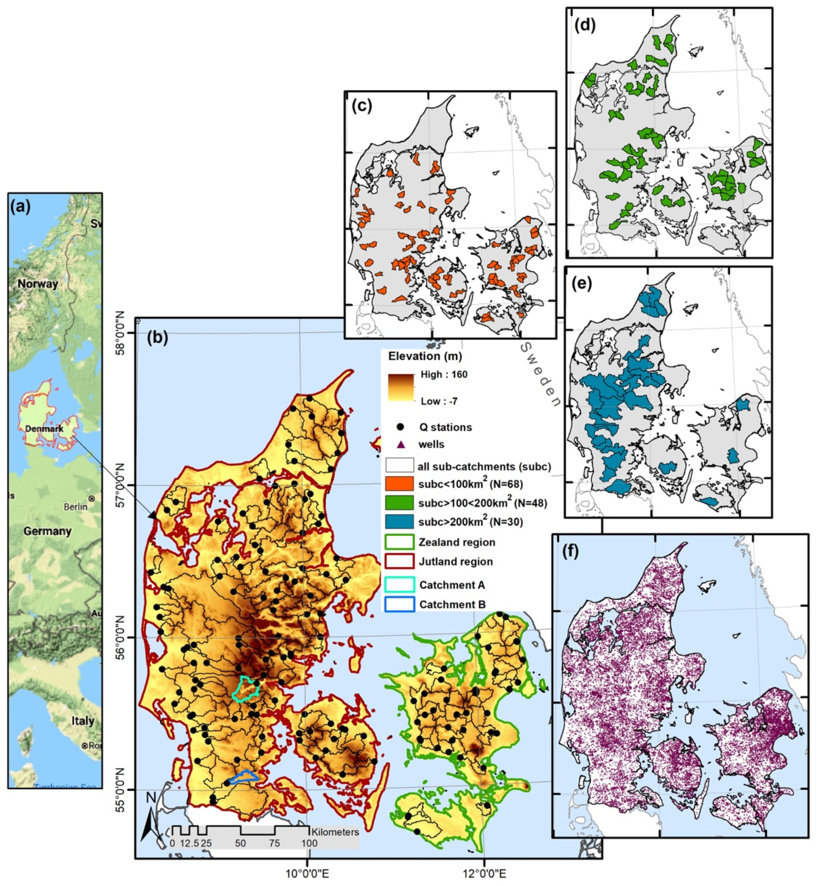
This study was performed for the land phase of Denmark. Figure 1b shows the study area and 146 incorporated discharge stations which are differentiated into downstream and upstream sub-catchments. The topography is generally flat where the highest elevation is up to 171 m a.s.l, and agriculture with more than 70% coverage is the main land cover type together with patches of coniferous and deciduous forests across Denmark. The eastern part of the country is dominated by a high fraction of clay soil, that is, >20% clay fraction; however, the western part is mainly covered with sandy soil i.e., <5% clay fraction (Figure 2a). The land-use is predominantly agriculture and the hydro-climate is dominated by energy-limited conditions in winter and most of autumn and spring, while the summer months can be water-limited. While, the lowest mean leaf area index (LAI) values with less than 2 m2/m2 are found in central Jutland [14] (Figure 2b), the highest mean land surface temperature (LST) values (approx. 290 K) are observed in south of Jutland (Figure 2c), see Figure 1b for the location of Jutland region. However, LST is consistently decreasing from southern to northern parts of Denmark.
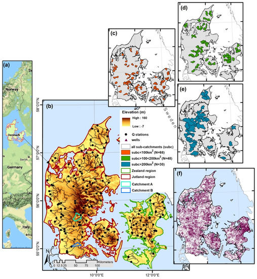
Figure 1.
Overview of the study area: (a) the geographical location of Denmark in northern Europe, (b) distributions of the selected 146 runoff gauges (Q stations) and two main administrative regions of Denmark with underlying topography, (c) sub-catchments (subc) smaller than 100 km2, (d) subc between 100 and 200 km2, (e) subc larger than 200 km2, and (f) a number of 25,981 hydraulic head observation wells used in the national water resource model of Denmark (DK-model) setup for modeling the groundwater flows.
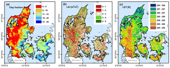
Figure 2.
The grid-cell (1 km) distributed annual mean (2002–2014) maps: (a) clay fraction, (b) leaf area index LAI, and (c) land surface temperature LST.
3. Data and Methods
3.1. Data
3.1.1. Water Balance ET Approaches
From a total dataset of 305 discharge stations (catchment size > 10 km2) including 126 downstream and 179 upstream sub-catchments in Denmark, 146 runoff gauges (Q-data) were considered in this study, which appropriately covers the entire country (Figure 1b). Observed runoff for a 13-year period of 2002–2014 was used in order to be in agreement with MODIS data. Our water balance ET analysis is also grouped according to the size of catchments (Figure 1c–e). A number of 68 out of 146 selected sub-catchments have <100 km2 (Figure 1c), 48 catchments range from 101 to 200 km2 (Figure 1d), and 30 are >200 km2 (Figure 1e). Most of the large sub-catchments are found in central parts of Jutland (see Figure 1b). In addition, we also estimated the regional WB ET pattern through aggregating the sub-catchments to 10 regions. The criteria for aggregation of the sub-catchments into regions were mainly based on the RS ET distributions to better understand similarities/dissimilarities between the WB/RS ET spatial patterns at a larger scale.
In terms of data availability, 73% (N = 107) of the catchments had a full length of Q-data (13 years). However, 9% (N = 13) and 18% (N = 26) had data-gaps ranging 2–6 years of records and 7–9 years of records, respectively. In addition, original Q values (m3 s−1) were converted to water depth (mm) through dividing by the sub-catchment areas (m2). Annual precipitation (P-data) for each sub-catchment was calculated using daily gridded data with a 10 km spatial resolution [58]. Due to the data comparability in water balance ET calculation, length of P-data corresponded to those of the runoff data for each year of records. The catchment-based P and Q data were used to calculate the standard surface WB ET by averaging over the years with available Q data. However, the standard WB ET method is modified by including the net intercatchment groundwater flow simulated by the national water resources model of Denmark (the DK-model) in the ET calculation. A detailed description on the DK-model is provided in Section 3.2.1.
3.1.2. Remote-Sensing ET Models
Three remote sensing ET estimates are used in this study, which are based on the moderate resolution MODIS data. With a spatial resolution of approx. 1 km and frequent data acquisition, the MODIS-based ET estimates can provide information at a relevant scale for Denmark and for optimization/evaluation of distributed hydrological models with a focus on spatial patterns of ET at the national scale for the future applications. Therefore, remote sensing-based ET models such as GLEAM [59] or the Meteosat-based LSA SAF ET [60] were not considered in this study as they do not provide the desired resolution. In addition, the focus of the current study is on the spatial patterns of ET, and therefore RS estimates that are not based on land surface models but confined to the available satellite observations and their spatial information content are preferred. The first of such estimate was obtained from the global MODIS16 ET product [61], which is originally based on the Penman–Monteith equation [62]; however, the model has been modified [40] to account for parameters not readily available from space [20]. The second one was obtained from the global PML_V2 ET product, which is a coupled diagnostic biophysical model [56]. The third was based on a two-source-energy-balance (TSEB) implementation for Denmark [14]. The TSEB ET product [57] is mainly driven by land surface temperature (LST), which is a key indicator of the evaporative state at the surface [63]. All datasets were resampled to 1 km grid cells, and monthly timescale over the period 2002–2014, covering the entire land phase of Denmark (see Figure 1b). We chose to neglect the short-term and inter-annual variability and instead investigate the spatial patterns of ET representing the average climatology, estimated as annual means. A summary of the remote-sensing ET products used in this study are given in Table 1.

Table 1.
Characteristics of three remote-sensing ET datasets used in this study. P-M: Penman–Monteith; GPP: gross primary production; P-T: Priestly–Taylor; FPAR: fraction of photosynthetically active radiation; GMAO: Global Modeling and Assimilation Office; GLDAS: Global Land Data Assimilation System.
3.2. Methods
The methodology employed to evaluate the spatial patterns and dependence structures in WB/RS ET products is presented as follows:
- Catchment water balance ET estimates from standard and modified approaches using groundwater net;
- Estimation of ET dependence structures using empirical Copula approach; and
- Assessment of ET similarity using a PCA analysis.
3.2.1. Catchment WB ET Estimates
We present two approaches for the ground-based ET calculation, i.e., standard and modified WB ET methods. In the standard WB ET approach, the ET rate for the years with P and Q data available for each sub-catchment was calculated. In this approach, both groundwater exchange (GWnet) and water storage changes () are ignored. On an annual to multi-annual timescale, can typically assumed to be negligible [17,22], however groundwater exchange flow can be considerable particularly for smaller catchments [25]. The standard WB ET () was defined as:
In the modified WB ET approach, in addition to the discharge measurement, the DK-model was used to estimate the net intercatchment groundwater flow to be included in Equation (1). The modified WB ET () was then defined as:
where is the net groundwater flow across the topographical catchment boundary, calculated as subtraction of the total groundwater boundary outflows from the total groundwater boundary inflows divided by the length of study period (2002–2014). For further descriptions, the MIKE-SHE graphical layouts representing the interrelationships between the water balance components, especially the intercatchment boundary flows applied in Equation (2) are provided in Appendix A.
To our best of knowledge, no study has included groundwater flows so far for estimating the surface WB ET. In the present study, we obtained the biweekly net groundwater estimates for both inflows and outflows of each catchment using the DK-model, which is operated by GEUS—Geological Survey of Denmark and Greenland [64,65,66]. The model is based on the MIKE-SHE modeling code [67]. MIKE-SHE is a physically-based distributed modeling system covering the entire land phase of the hydrological cycle [67,68], which describes a full 3D finite difference groundwater flow, 1D unsaturated flow and 2D overland flow in separate modules that are coupled two-ways in every time step. For detailed description on the model code, it is referred to (e.g., [65,68,69]).
Groundwater abstraction plays a major role in the groundwater hydrology of Denmark, and a total number of approximately 40,000 abstractions wells for domestic/industry and irrigation are included in the DK-model setup, accounting for the entire groundwater abstraction in Denmark. Therefore, our modified WB ET approach covers both human (anthropogenic activities on irrigation and ground water extraction) and natural (net interbasin groundwater flows) impacts on the water balance closure. However, the groundwater boundary flows may largely be driven by the natural part, i.e., geology, in Denmark.
The DK-model is a fully distributed grid-based flow model setup in a 500 m resolution for the entire surface area of Denmark (43,000 km2) and run on a daily time step. The model structure is based on a comprehensive hydro-stratigraphic model for Denmark and parameterized through calibration against objective functions based on 305 discharge stations and 25,981 hydraulic head observation wells for the period 2000–2010 (for the current application run for the period 2002–2014). The main objective functions are Kling–Gupta efficiency (KGE) [70] and percent bias (Pbias) for streamflow, and continuous ranked probability score (CRPS) values for groundwater heads [53]. Details on the model data, construction, calibration, and validation can be found in [71], while calibration statistics will be presented in brevity in the Result section.
3.2.2. Empirical Copula-Based ET Dependence Structures Analysis
To capture the underlying dependence structures amongst the WB/RS ET products, the empirical Copula function was applied. The Copula approach [72] states that any multivariate distribution function can be decomposed into the marginal distributions and a Copula, which the dependence structure between variables is appropriately estimated [73]. The separated analysis of marginal distributions and dependence structure (i.e., the Copula) is one of the major benefits of using Copula functions to describe joint distributions between variables [74].
In this study, it was essential to obtain the joint probability distribution function between the ET products used. While marginal distributions of such datasets are commonly known, their joint distributions are typically too complex to appropriately derive from the marginal distributions [75]. Therefore, empirical Copula was employed herein to estimate their joint distributions. Moreover, the pairwise dependence between such variables has been traditionally described using classical families of bivariate distributions such as normal, gamma, and Gaussian distributions. The main limitation of this approach is that the individual behaviors of the two variables or transformations thereof need to be then characterized by the same parametric family of univariate distributions [76]. As a result, distributions of these statistical-based methods remain symmetrical, meaning that it is not clear whether correlations and dependencies are stronger/weaker at low, high, or middle-range of values. Copula functions, however, avoid this restriction. This implies that Copula-based distributions are asymmetrical, in such a way it indicates which part of the datasets are highly/weakly correlated i.e., at lower—or upper tails.
Here, a two-step approach was applied to estimate the Copula density . First, , of the marginal distributions was obtained using the empirical distribution function as an estimator. Second, the pseudo-observations were defined [77]. The Copula density, which is purely based on the real data [78], was finally estimated as the joint density of . If and denote marginal distributions-based rank space values, the empirical Copula was then defined as:
where and is the indicator function that takes a value of 1 if the argument is true) and being the sample size. For detailed information about Copulas, it is referred to e.g., [73,75].
3.2.3. PCA-Based Similarity Assessment of ET Products
To assess the similarity and rank WB/RS ET products used, a principal component analysis (PCA) was performed. It is a linear algebra-based multivariate procedure that summarizes the information in a dataset. PCA rotates the axes so that the new coordinate system aligns with the orientation of maximum variability available in the dataset. The rotation is a linear transform and the new coordinate axes are then a linear combination of the original axes. This approach allows to discard components that contribute insignificantly to describe the variability in the data. Therefore, insignificant dimensions can be removed from the rotated space (i.e., PCA-transformed space) without affecting relationship of the remaining components. The space is yet linear, but dimensionality of the multivariate dataset is reduced [12,79]. We achieved this by transforming the input ET datasets into a new small set of datasets without losing the most important information in the original data. These new datasets correspond to a linear combination of the originals and are called principal components (PCs). The PCs are ranked in that way that PC1 explains the largest fraction of the variance in a dataset, PC2 the second largest, etc. For a full description on the procedure of PCA technique, it is referred to e.g., [80,81].
4. Results and Discussion
4.1. Remote-Sensing Derived Evapotranspiration
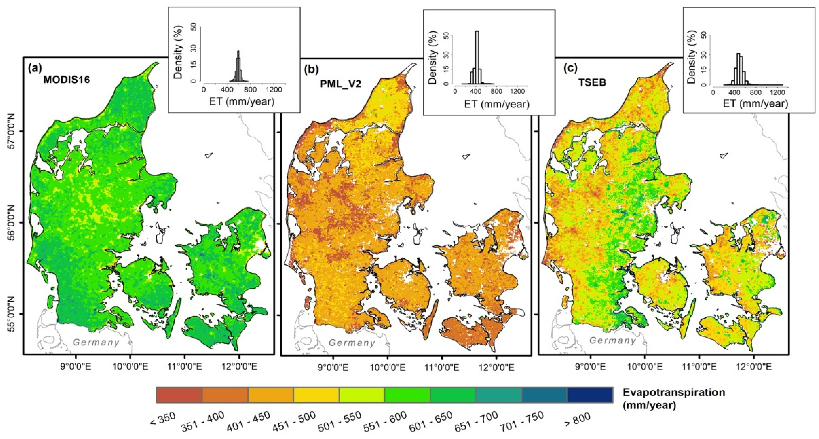
The grid-based mean annual ET values derived from RS models of MODIS16, PML_V2, and TSEB, together with their probability density estimations (histograms), are shown in Figure 3. It can be seen that in general, the RS ET patterns vary to a large extent. Low values of the MODIS16 ET less than 450 mm/year are spatially limited, and mostly found in central Jutland (see Figure 1b for location of the region), while the rest of the country indicates a consistent pattern with higher ET rates, for which maximum values (>700 mm/year) are observed in southwestern Jutland (Figure 3a). Likewise, PML_V2 ET low values (<350 mm/year) are mainly observed in central Jutland, and the higher ET values (>450 mm/year) seen in the north and southern parts of Jutland (Figure 3b). Therefore, MODIS16 and PML_V2 show a very similar ET spatial patterns; however, they vary in terms of absolute values. On the contrary, TSEB indicates a different ET spatial pattern across the country (compared to MODIS16 and PML_V2). The low values (<450 mm/year) are distributed in most regions except for the eastern Jutland, where higher values above 600 mm/year are found. Some regions in the northeast part of Zealand (see Figure 1b for location of the region) also show high values (Figure 3c). The highest ET difference between the three RS estimates are found over the eastern/western Jutland with a value of approx. ±350 mm/year (not shown). Overall, MODIS16 and PML_V2 represent a relatively uniform spatial pattern with a narrower range of values (440–757 and 186–711 mm/year, respectively) compared to TSEB, which shows a sharp contrast between eastern and western parts of the country with a broader range of values (248–1289 mm/year). This is demonstrated by the underlying distributions of the RS ET histograms, as well (Figure 3).
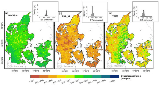
Figure 3.
Grid-based satellite remote-sensing evapotranspiration (RS ET) distributions (1 km spatial resolution) along with the histogram of the mean annual ET (50 mm/year bins): (a) MODIS16, (b) PML_V2, and (c) two-source energy balance model (TSEB). The urban areas have been masked out in the maps (see Figure 2a for details).
4.2. Catchment Water Balance ET
The spatial distributions of annual mean precipitation and surface streamflow are shown in Figure 4a,b, respectively. It can be seen that the measured discharge demonstrates a similar pattern as the observed spatial pattern of precipitation, in such a way that both are decreasing from western (P > 900 mm/year and Q > 500 mm/year) to eastern (P < 600 mm/year and Q < 200 mm/year) parts of Denmark. The Q pattern is also captured by the runoff-ratio map (see Appendix B). Typically, the runoff ratio, which is the proportion of P that is not taken up by ET and which eventually generates runoff at the catchment outlet, is controlled to some extent by land surface-based variables such as soil type and soil texture, so that soils containing large fraction of clay infiltrate less water than sandy soils and thus produce higher runoff ratios. However, this is not the case in our study area. In fact, runoff generation in Denmark insignificantly affected by clay fraction, but mainly follows the input precipitation pattern (see Figure 2a for distribution of the clay fraction).
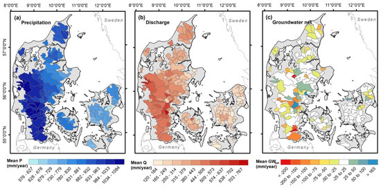
Figure 4.
Catchment-based annual mean maps: (a) observed precipitation, (b) measured surface streamflow, and (c) modeled groundwater net (negative values indicate loosing conditions i.e., boundary outflow). All units are in mm/year.
In addition to P and Q data as routine components for calculating surface WB ET, in this study, we also considered the groundwater boundary flows in order to modify the standard ET calculation (see Equations (1) and (2)). Figure 4c displays the spatial pattern of annual mean values for the groundwater net data simulated by the DK-model. Further, 35% of the 146 sub-catchments show a loosing condition with values ranging from −25 to −200 mm/year; however, only 5% indicate high negative values less than −150 mm/year. On the contrary, 10% (3% > 100 mm/year) of the catchments have a positive net groundwater exchange with values ranging from 25 to 165 mm/year. Overall, most of the sub-catchments (55% of all) show a rather small range of values i.e., ±25 mm/year. Interestingly, the larger catchments (>200 km2) generally display lower inflow/outflow values compared to the smaller catchments. This implies that larger basins have a tendency to less errors and uncertainties in terms of water balance closure using the standard WB ET assumption. Similar results were also reported by e.g., [5]. Further discussion about the effect of catchment size on the water balance ET estimates is provided in the follow-up section.
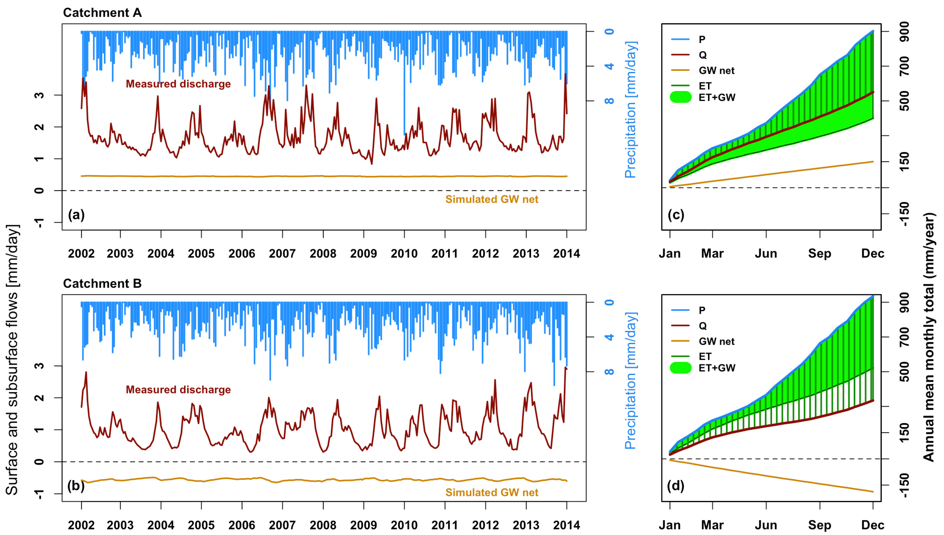
To further investigate and demonstrate the importance of adding the long-term mean GW-net data in the surface water balance ET calculation, we illustrate a two-week-interval timeseries (Figure 5a,b) and long-term monthly mean cumulative distribution of the water balance components (Figure 5c,d) for two selected catchments, A and B (see Figure 1b for the location). Two criteria were applied for the selection of these catchments: (i) having full data coverage (13-year), and (ii) being extreme cases for both groundwater (GW) inflow (positive) and outflow (negative) conditions. The measured P timeseries shows limited seasonality and inter-annual variability. The measured Q followed P peaks in wintertime for both catchment A and catchment B. In Denmark, high discharge typically occurs during wintertime as a consequence of low potential ET and above average precipitation. It can be seen that temporal (annual/inter-annual) variations in the simulated GW-net timeseries are very low, for both inflow/positive and outflow/negative conditions (Figure 5a,b, respectively). However, despite low values especially for net inflow (Figure 5a), GW-net data closely follow the seasonality of Q. This implies that, peak discharge values are appropriately corresponded to the high values of GW-net inflow.

Figure 5.
(a) Two-week-interval timeseries of the measured discharge (Q) and simulated groundwater net (GW-net), and (c) annual mean monthly totals of precipitation (P), Q, GW-net, surface water balance evapotranspiration (WB ET), and surface WB ET plus GW-net (ET + GW) for catchment A. (b,d) the same as in (a,c), but for catchment B. In the graph, positive (negative) values of GW-net indicate inflow (outflow). The units for a/b and c/d are mm/day and mm/year, respectively. To see the locations of catchments A and B, it is referred to Figure 1b.
In addition, the long-term monthly mean (2002–2014) water balance components of P, Q, GW-net, ET, and ET plus GW-net data used in the modified WB ET calculation (see Equation (2)) for inflow and outflow conditions are shown in Figure 5c,d, respectively. The surface ET estimate, as shown in catchment A, is greatly increased (approx. 17% total) after adding GW-net flow to WB ET calculation in inflow condition (green shaded area in Figure 5c). In contrast, it is notably decreased (approx. 21% total) when GW-net is subtracted from the WB ET in catchment B in outflow condition (green shaded area Figure 5d). Therefore, based on data presented in Figure 5, it becomes clear that the WB approach to estimate ET cannot be applied at shorter timescales than the long-term annual mean, as water balance closure cannot be granted at shorter timescales. This, thus highlights that the long-term annual mean GW-net data could have a considerable contribution to accurately estimate water balance ET, especially in small-scale catchments with a complex geology. To see a graphical water balance condition for the catchment A and catchment B, it is referred to Appendix A.
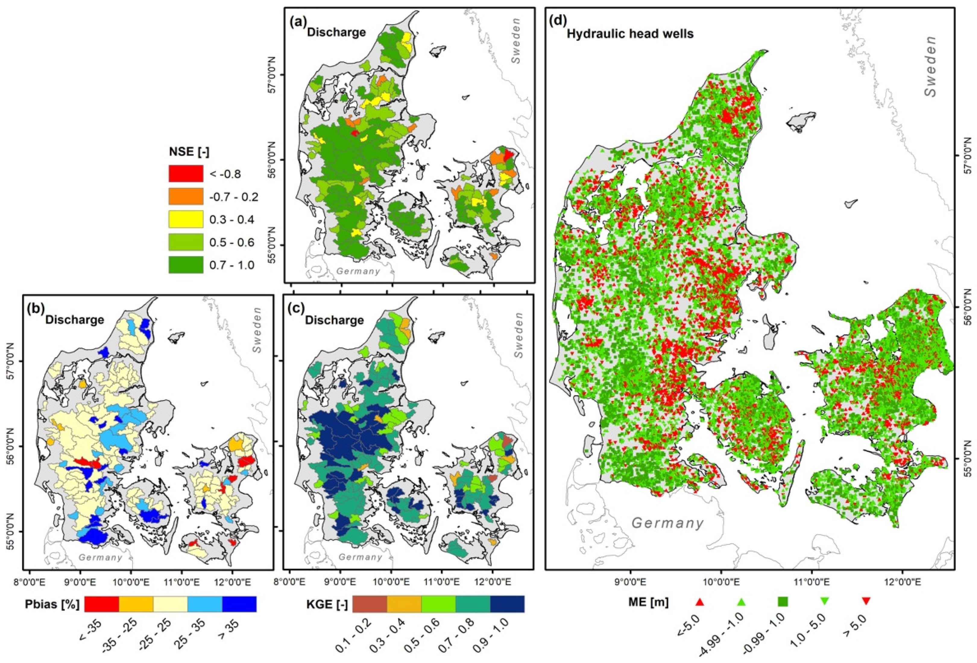
To examine the accuracy and robustness of the DK-model, its performance was evaluated for the period 2000–2010 against observations of discharge (Figure 6a–c) and hydraulics head wells (Figure 6d) using multiple statistical metrics across the study area (see Figure 1 for more details). For discharge, most of the catchments indicate a high Nash–Sutcliffe efficiency (NSE > 0.6) (Figure 6a) and low Pbias < 25% (Figure 6b). The high capability of the DK-model to reproduce discharge is also confirmed by a high values of KGE > 0.7 (Figure 6c). Nevertheless, the model shows some limitations to accurately simulate the surface streamflow especially in smaller catchments, where the lowest/highest efficiency/error is observed; however, these errors/shortcomings can be insignificant as limited to fewer catchments at the national scale of Denmark. With regard to the hydraulics head wells, as shown in Figure 6d, the model shows a reasonable performance also. The majority of the head wells are well reproduced by the model with an approx. 1 m error; however, the error is rather high in some wells (>±5 m) especially in eastern part of the Jutland, mainly due to a more complex geology and higher elevation gradient (see Figure 1b for location of the region). Overall, the DK-model indicates a good performance to model the surface/subsurface flows, mainly because of an abundant and rich observational input data used in the model setup (see Section 3.1.1 and Section 3.2.1 for further details).

Figure 6.
The DK-model performance’s statistical metrics: between the observed and modelled discharge for (a) Nash–Sutcliffe efficiency (NSE), (b) Pbias, (c) Kling-Gupta efficiency (KGE), and between the observed and modelled hydraulic head wells for mean error (ME) (d).
4.2.1. Spatial Comparisons of WB/RS ET Products
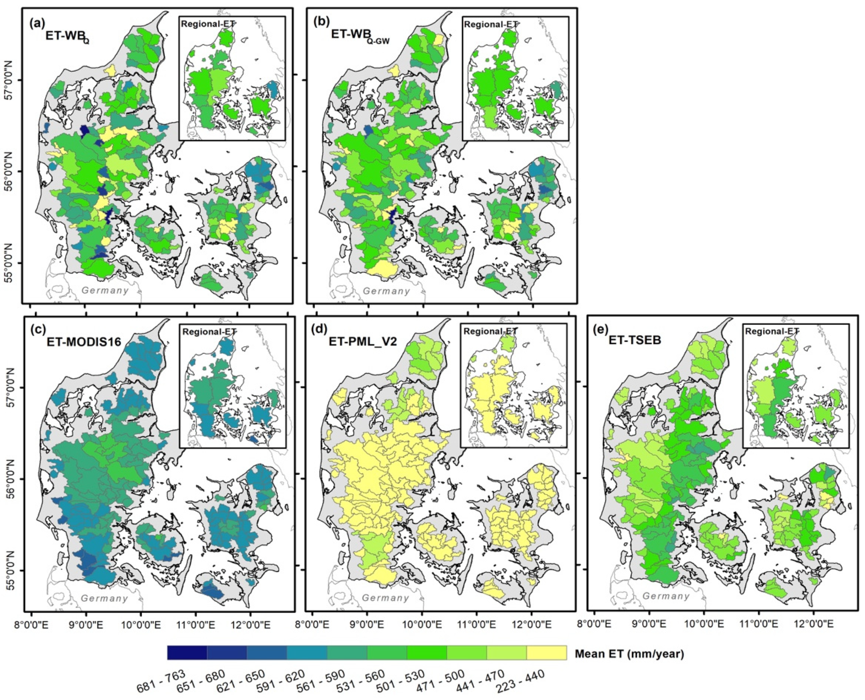
Figure 7 presents the catchment-based annual mean spatial patterns together with the regional estimations of ET datasets from standard WB ET and modified WB ET approaches as well as RS ET models of MODIS16, PML_V2, and TSEB. The spatial distribution of the standard water balance evapotranspiration approach (ET-WBQ), unlike the Q pattern, does not show a clear ET pattern across the study area (Figure 7a). In other words, ET-WBQ indicates a large spatial discrepancy with regards to Q over Denmark (see Figure 2b and Figure 4b). High ET values (>600 mm/year) are mainly distributed in a few small-scale catchments in the central parts of Jutland (see Figure 1b for the location). However, based on the spatial information presented in Figure 1b and Figure 4a, these high values cannot be merely due to high precipitation and underlying topography. In order to shed light into those extreme ET values in some sub-catchments, we modified the standard ET calculation (Equation (1)) through including the net groundwater data (Equation (2)). The spatial pattern of the modified water balance evapotranspiration approach (ET-WBQ-GW) is illustrated in Figure 7b. The result verifies the fact that the ET pattern is smoothed, meaning that very high (unusual) ET values for some smaller catchments are now modified. However, the DK-model indicates limitation to fully eliminate discrepancies in the ET patterns for all sub-catchments with unusual high and low ET values. Nevertheless, the results (Figure 7a,b) indicate the importance of adding groundwater data for an accurate water balance condition with a focus on ET estimation. This was also highlighted by other researchers e.g., [25,27,28].
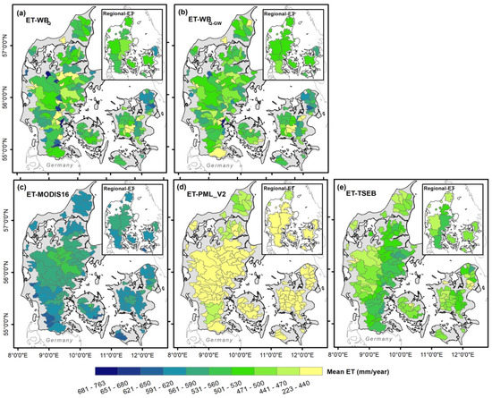
Figure 7.
Catchment-based comparison of annual mean ET patterns: (a) standard WB ET, (b) modified WB ET, (c) MODIS16 ET, (d) PML_V2 ET, and (e) TSEB ET. The small panels indicate aggregated sub-catchments (N = 10 out of 146) for calculation of the regional ET patterns for each ET dataset.
The remote sensing MODIS-based ET datasets derived from MODIS16, PML_V2, and TSEB algorithms were evaluated using the modified WB ET. With reference to ET-WBQ-GW, the results (Figure 7c–e) indicate that the three RS ET spatial patterns largely vary compared to the reference ET, and practically, there is almost no consistency and relationship between RS and WB ET maps. Notable differences are mainly observed in eastern Jutland (see Figure 1b for the location) for TSEB with high values above 560 mm/year, whereas MODIS16 and PML_V2 are spatially distributed with values ranging 530–650 mm/year and 250–450 mm/year, respectively across the country. Overall, such spatial discrepancies in the ET datasets reveal high levels of uncertainties, not only for the three RS models, but also for the reference WB approach. However, even though the spatial patterns of catchment-based ET products are largely dissimilar at the national scale, their specific estimates for particular regions are fairly consistent. Compared to ET-WBQ-GW, both MODIS16 and TSEB are in relatively good agreement for some regions in northern/southwestern Jutland and northern/central Zealand (see Figure 1b for the locations). Accordingly, the regional ET spatial patterns also indicate a more similar pattern (regardless of the absolute values) amongst ET datasets when individual catchments (N = 146) were aggregated into a few larger regions (N = 10); this, is more evident between ET-WBQ-GW and MODIS16 (small panels in Figure 7b,c).
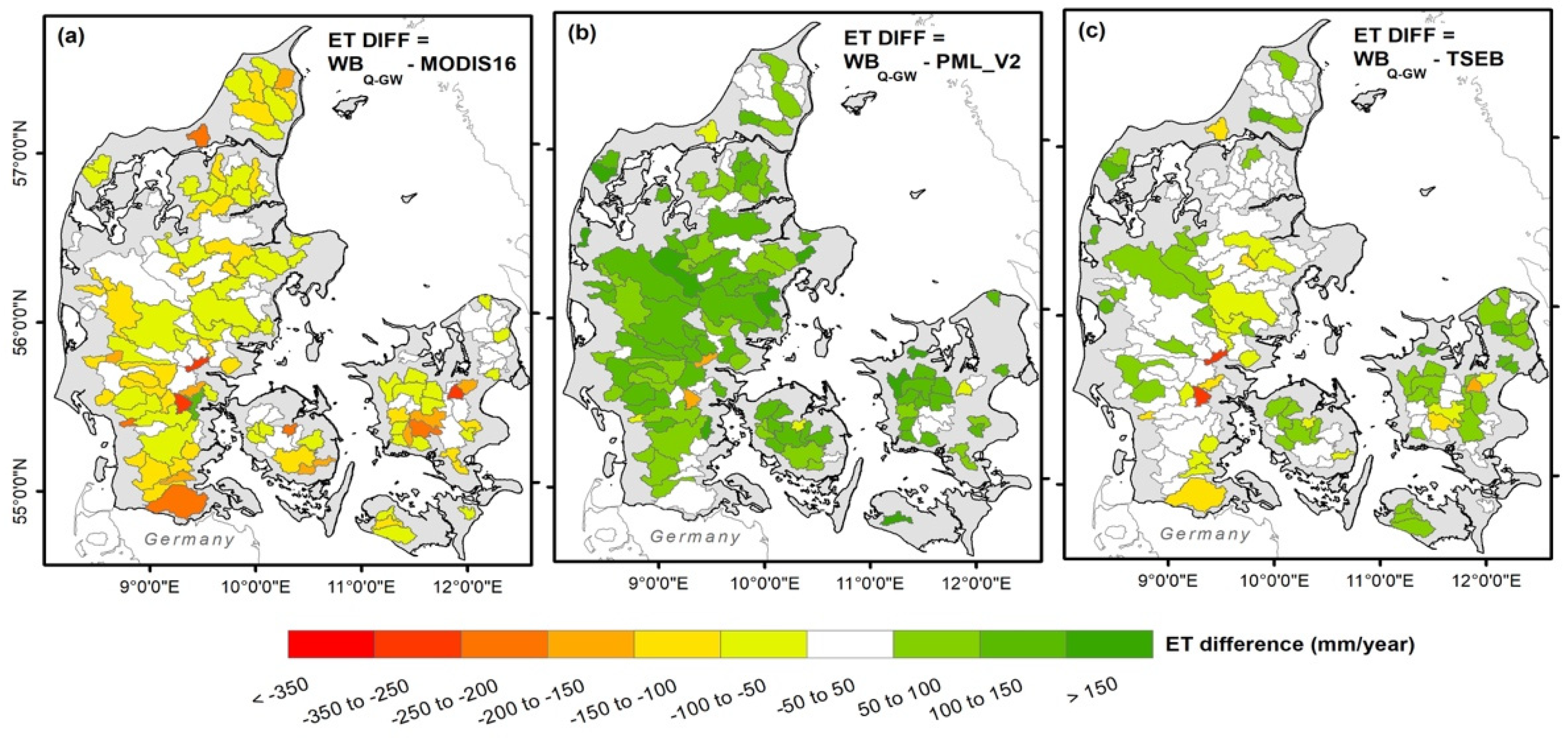
Besides the analysis of ET spatial patterns, ET differences (∆ET) between ET-WBQ-GW and RS ET models were also investigated. The results are shown in Figure 8. It is observed that spatial distributions of ∆ET are weakly consistent among the three MODIS-based ET algorithms. However, number of sub-catchments with very high ∆ET values >−250 mm/year are limited to approx. In addition, 3% of the catchments are mostly observed in central parts of Jutland and Zealand (see Figure 1b for the location). A closer examination revealed that large negative ∆ET is mainly found in the regions with rather high P and Q values (see Figure 4), for which resulted in a lower WB ET rate over the corresponding catchments (see Figure 7b). In contrast, many catchments have rather small ∆ET values ranging between −150 and 150 mm/year (~90% of all). This suggests that, despite a large discrepancy among the ET spatial patterns at the national scale, MODIS-based ET models agree fairly well with ET-WBQ-GW for a majority of the catchments.

Figure 8.
Maps of the differences between the sub-catchment ET (mm/year) from the modified water balance method (WBQ-GW), and the remote-sensing models of MODIS16 (a), PML_V2 (b), and TSEB (c).
Seemingly, as shown in Figure 8, largest ∆ET either negative biases (RS ET overestimates) or positive biases (RS ET underestimates) are mainly found for smaller catchments. It was further analyzed and illustrated in Figure 9, which ranked catchments by their ∆ET for varying catchment sizes. Interestingly, it turned out that ∆ET magnitudes between RS and WB ET methods are clearly decreased from small catchments below 100 km2 (>−300 and <250 mm/year) to larger catchments above 200 km2 (>−150 and <180 mm/year). MODIS16 (Figure 9a), however, shows a clearer decreasing trend (with an overestimated rate) compared to PML_V2 (Figure 9b) and TSEB (Figure 9c). Further, the aggregated regional-scale ∆ET magnitudes are even further decreased (compared to catchment size-based ∆ET), in particular for MODIS16. This analysis, therefore, highlights that RS MODIS-based ET spatial errors and uncertainties can be much higher for small-scale, energy-limited areas (like over Denmark applied in this study) compared to much larger regions such as over the United States e.g., [5] or Canada e.g., [20], which both reported a high reliability of the RS ET products for catchment-based ET estimation at larger catchments.

Figure 9.
Catchment size-based ET differences between the modified surface WB method and RS ET models of (a) MODIS16, (b) PML_V2, and (c) TSEB. Different point symbols of filled circle, square and triangle (star) on the lines represent individual catchment (aggregated catchment). For more information about the size and numbers of the sub-catchments, it is referred to Figure 1.
4.3. Dependence Structures of ET Products: Copula-Based Analysis
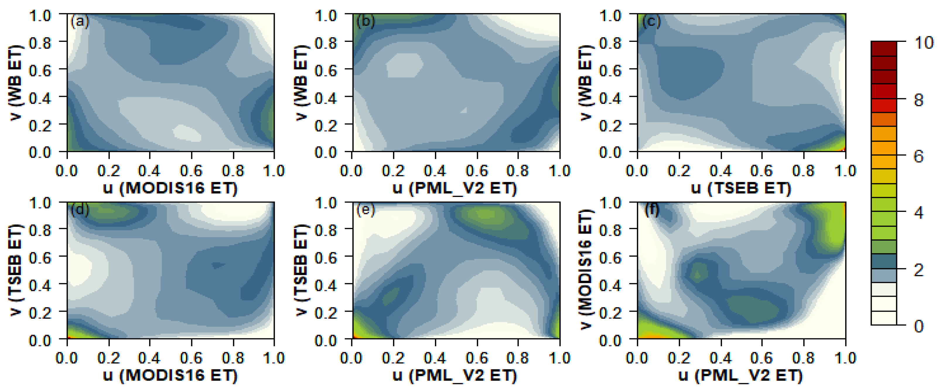
The empirical Copula densities amongst the WB ET and RS ET products are illustrated in Figure 10. In general, the RS ET products from MODIS16 (Figure 10a) PML_V2 (Figure 10b) and TSEB (Figure 10c) algorithms do not show a significant dependence structure against the modified WB ET. Instead, a nonlinear structure of the joint relationship between the ET products is observed with strongly varying densities in the different percentiles. The Copula density of WB and versus MODIS16 and PML_V2 indicates a complex, but partially positive relationship with multiple densities; in contrast, it is clearly asymmetrical with the highest densities in lower-right tail between the WB and TSEB showing a strong negative correlation. However, unlike catchment-based WB/RS ET dependencies (Figure 10a–c), the grid-based dependence structures of three remote-sensing ET datasets are stronger and clearer (Figure 10d–f). Copula densities between RS ET products are asymmetrical. This implies that, the highest dependency is seen in the lower-left corner, where the low values are found between MODIS16/TSEB (Figure 10d) and PML_V2/TSEB (Figure 10e). Thus, they are strongly concordant in the lower ranks of the distribution only. Further, a second maximum density can be observed between higher and lower (and upper) ranges of TSEB and MODIS16 (and PML_V2). However, PML_V2 and MODIS16 indicates a significant symmetric dependence structure with maximum densities in the lower-left and upper-right corners. This means that, highest correlation is found at both low and extreme values (Figure 10f).
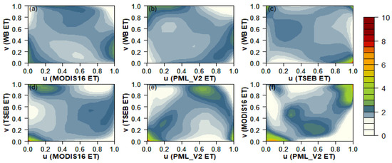
Figure 10.
The empirical Copula densities between the satellite RS ET products and surface WB ET estimate. The sample size is 146 (20,654) data tuples in (a–c) in (d–f) panels for the ET datasets. Panels (a–c) indicate the dependence structure pattern of the water balance ET against the three derived remote sensing ET products estimated at catchment-scale (as in Figure 7); while panels (d–f) indicate the dependence structures amongst the three remote sensing ET estimated at pixel-by-pixel for the entire domain (as in Figure 3).
Therefore, a complex and nonlinear dependence structure pattern achieved by the Copula analysis amongst WB/RS ET products, may partially explain large discrepancies observed in the ET spatial patterns (Figure 7) applied at the national scale of Denmark. Additionally, Copula-based dependence structures between the ET estimates against land-surface/climate variables were estimated also. Overall, the WB/RS ET products indicated a stronger correlation and clearer dependence structure pattern to the land-surface variables (i.e., clay fraction, LST, and LAI) compared to the meteorological variables (i.e., precipitation, air temperature, solar radiation, and wind velocity) over Denmark with a predominantly energy-limited environment. A further detailed description is provided in Appendix B.
4.4. Similarity Assessment of ET Products: PCA-Based Analysis
To assess the similarity ranking amongst the ET estimates, we performed a PCA analysis for both grid-based RS ET (Figure 11a) and catchment-based WB/RS ET (Figure 11b) products. The three remote-sensing ET datasets from MODIS16, PML_V2, and TSEB algorithms are positively correlated to PC1. This implies that, in general, the RS ET products show some degrees of similarity. However, MODIS16 and PML_V2 indicates a closer spatial pattern compared to TSEB; this becomes more apparent in PC2 (Figure 11a). The catchment-based PCA results also show that the water balance and three MODIS-based ET products, as illustrated in Figure 11b, differ to a large extent. Nevertheless, WB ET and MODIS16 ET estimates, unlike PML_V2 and TSEB, shows a closer spatial pattern. In both PC1 and PC2, TSEB shows a strong negative correlation to WB, indicating a higher spatial discrepancy when compared to MODIS16, PML_V2, and WB ET spatial maps (see Figure 7). These results are in good agreement with those captured by the Copula analysis (see Figure 10).
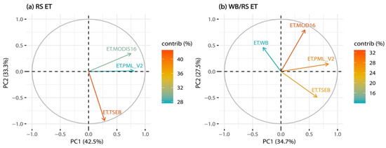
Figure 11.
Principal component analysis PCA-based ET similarity assessment: inter-correlations between RS ET algorithms (a) and WB/RS ET products (b). The sample size is 20,654 (146) data tuples in (a,b) panel for the ET datasets.
4.5. ET Uncertainties
For calculation of the surface water balance ET, we used both standard (ET = P − Q) and modified (ET = P − Q + GWnet) approaches. Generally, the errors associated with precipitation P and runoff Q may have large effects on WB ET estimates [5]. In this study, gridded daily P data with a 10 km spatial resolution [58] was used. The daily station series was quality tested by the Danish Meteorological Institute (DMI), however, no testing for homogeneity has been performed on P daily observations [82]. Additionally, discharge stations used are part of the Danish river monitoring network. Although this network covers Denmark appropriately and its monthly runoff data are qualified, it is not without limitations. For example, the streambed profile of the streams at some stations in central Jutland (see Figure 1 for the location) are considered unstable due to a significant growth of vegetation in summertime [83]. Therefore, these, might be some sources of error in in situ observations.
The annual mean WB ET estimated based on the modified approach (ET-WBQ-GW) (Figure 7b) reduces the spatial variability, seemingly improving the realism of the spatial pattern compared to the standard procedure (ET-WBQ) (Figure 7a), due to the inclusion of GW-net in the ET calculation. This accounting for GW-net, separates this study from the previous studies applying WB ET calculation at the catchments scale while neglecting GW-net by treating it as a source of uncertainty e.g., [5,17,55]. However, despite being included herein, the modified WB ET still shows a heterogeneous spatial pattern across the study area with extreme variability among neighboring catchments. This indicates that even when accounting for GW-net estimates from a calibrated regional/national groundwater flow model, the uncertainties associated with the WB ET method for relatively small catchments is still significant. Additionally, estimates of GW-net from the DK-model simulations are subject to error and uncertainty and as a consequence, an unrealistic spatial pattern of ET-WBQ-GW remained (Figure 7b). Hence, we speculate that errors have not been fully eliminated in the ET-WBQ-GW approach and that there is a limitation to the WB ET approach that increases with decreasing catchment size.
The uncertainty associated with remote-sensing ET estimates is generally difficult to identify due to different input data [84] leading to large uncertainties in forcing and ancillary data [85], different algorithms and methods for ET estimation [35], different parameterizations [5], and different spatiotemporal resolution of the input dataset [86]. However, despite the fact that all the three RS MODIS16, PML_V2, and TSEB ET algorithms used in this study are based on MODIS data (see Table 1 for details), they largely differ not only in their absolute values, but also spatial patterns at the national scale of Denmark. As a result, a large spatial discrepancy was observed between the WB ET and RS ET models applied (Figure 7); this was also highlighted by the Copula analysis, of which a different underlying dependence structure was captured between the ET products (Figure 10). These findings separate this study from most previous studies of similar nature, where typically strong correlation coefficients (best fit) for RS/WB ET datasets were reported, most probably due to the large spatial variability in climate, elevation, aridity etc. resulting from continental scale applications.
In addition, the catchment-scale errors in MODIS16, PML_V2, and TSEB ET estimates with respect to ET-WBQ-GW was found to be on average 18.7% (ranged between 0.04% and 147%), 20.4% (ranged between 0.56% and 72%), and 12.8% (ranged between 0.27% and 142%), respectively. Moreover, catchment-size and regional analyses indicated that errors and uncertainties of WB ET against RS ET methods are clearly decreased for larger catchments and regions (Figure 9), which was also reported by other researchers e.g., [5,20]. Therefore, these indicate that application of remote-sensing ET products, even from similar algorithms, could be challenging over small-scale, high-latitude, and energy-limited regions like Denmark applied in this study. Thus, satellite RS data may need a bias correction to be performed prior to application over such regions. As indicated by [5], in dry regions, ET is generally controlled by water availability as most input precipitation on the surface is converted to ET and only a small portion generates runoff, thus ET models can capture the spatiotemporal variability more accurately; by contrast, in humid areas ET is mainly controlled by energy and vegetation; and thus spatiotemporal variability of ET is lower and more difficult to capture. Overall, the spatial pattern of MODIS16 ET, as captured by the PCA analysis (Figure 11b), is closer to the reference water balance ET pattern as compared to the PML_V2 and TSEB patterns over Denmark.
5. Conclusions
The main conclusions of this research can be summarized as follows:
- The ET-WBQ spatial patterns indicated a significant inconsistency over Denmark, with an energy-limited environment; however, it was improved especially for smaller catchments, when GW-net data was included in the ET-WBQ-GW estimate. Nevertheless, there is still challenges in applying the WB ET approach to small regions.
- The TSEB, MODIS16, and PML_V2 ET estimates varied largely compared to ET-WBQ-GW; as a result, a large discrepancy was observed amongst the ET products at the national scale of Denmark. However, many catchments had ∆ET < ±150 mm/year. Regional analysis also indicated that RS ET uncertainties decrease with increasing catchment size.
- The Copula analysis captured a nonlinear structure amongst the ET products with multiple densities (either in lower or upper ranks), showing a complex relationship between not only the RS ET datasets, but also between ET-WBQ-GW and MODIS-based ET products. The ET-WBQ-GW and MODIS16 ET showed a closer spatial pattern as identified by PCA analysis, indicating a good potential for future applications over the study area.
- Finally, it is recommended that for WB ET calculation, future studies should incorporate GW-net from surrogate hydrological models if available. In addition, Copula approach can be considered in other catchments worldwide for estimating true relationships amongst water balance (or energy balance) components in addition to traditional statistical analyses.
Author Contributions
Conceptualization, M.S., S.S. and J.K.; methodology, M.S., J.K. and S.S.; software, M.S. and S.S.; validation, M.S., J.K. and S.S.; formal analysis, M.S. and S.S.; investigation, M.S., S.S. and J.K.; resources, M.S., J.K. and S.S.; data curation, M.S. and J.K.; writing—original draft preparation, M.S.; writing—review and editing, M.S., J.K. and S.S.; visualization, M.S.; supervision, S.S.; project administration, S.S.; funding acquisition, S.S. All authors have read and agreed to the published version of the manuscript.
Funding
This research was funded by Villum Foundation, grant number VKR023443.
Data Availability Statement
The remote sensing ET models derived from MODIS16 and PML_V2 algorithms used in this study are publicly available. However, the TSEB RS ET model as well as the water balance ET datasets are available upon request.
Acknowledgments
The authors would like to acknowledge the financial support received for the SPACE project provided by the Villum Foundation (http://villumfonden.dk/) (accessed on 30 September 2020) through their Young Investigator Program (grant VKR023443).
Conflicts of Interest
The authors declare no conflict of interest.
Appendix A Water Balance Visualization
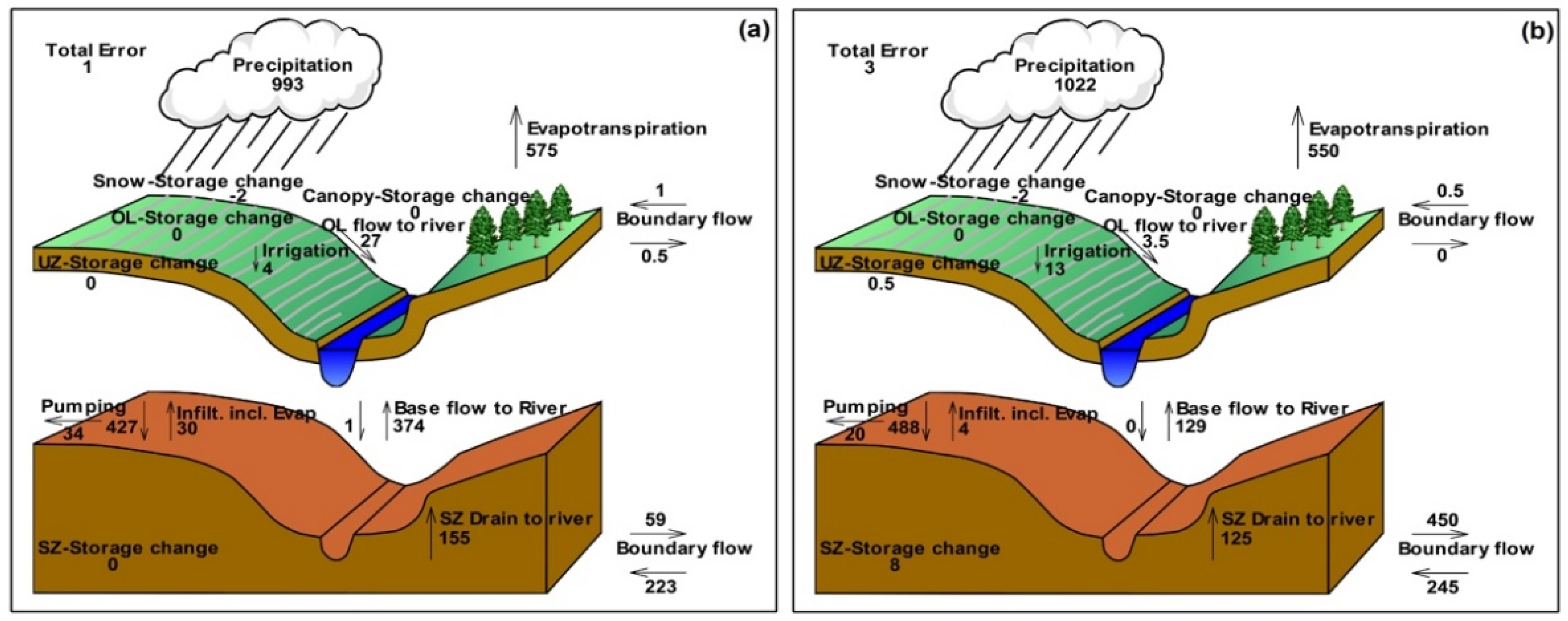
Figure A1 illustrates the graphical water balance outputs form MKE-SHE simulations for catchment A (Figure A1a) and catchment B (Figure A1b) in the extreme positive and negative boundary flows conditions, respectively; see Figure 1b for the location of the catchments. The interrelationships between the various water balance components, in particular, the intercatchment boundary flows in the unsaturated zone UZ and saturated zone SZ are clearly visualized (Figure A1). This highlights the importance of add of net intercatchment groundwater flow (GW-net) in the long-term annual mean water balance ET calculation, unlike to UZ/SZ storage changes that can be negligible.
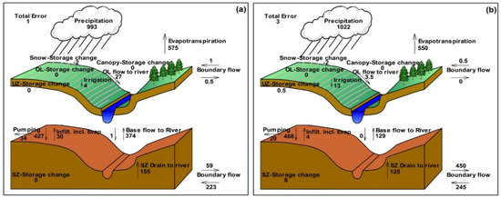
Figure A1.
The MIKE-SHE graphical water balance output: (a) for catchment A (which, is a positive/inflow condition) and (b) for catchment B (which, is a negative/outflow condition) for the period 2000–2010, see Figure 1b for the location of the catchments. In the graph, inflows (out-flows) to (out of) the catchment are illustrated as leftward (rightward) arrows. The unit is mm/year in all the variables. OL: overland, UZ: unsaturated zone, and SZ: saturated zone.
The runoff ratio map, which was calculated by dividing discharge (Figure A2b) to precipitation (Figure A2a) is shown in Figure A2d. It can be seen that the catchment-based spatial patterns of the calculated runoff ratio and the measured discharge are very similar. This indicates that the surface streamflow is mainly driven by the input precipitation pattern (Figure A2a), but not much by the clay fraction content (see Figure 2a) over Denmark. It is noted that, Figure A2a–c are again represented here for convenience’s sake, when all directly compared with the runoff ratio map.
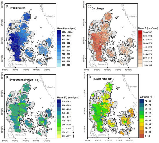
Figure A2.
The catchment-based annual mean maps: (a) observed precipitation, (b) measured su face streamflow, (c) water balance evapotranspiration, and (d) the runoff ratio map (discharge/precipitation).
Figure A2.
The catchment-based annual mean maps: (a) observed precipitation, (b) measured su face streamflow, (c) water balance evapotranspiration, and (d) the runoff ratio map (discharge/precipitation).

Appendix B Copula-Based Dependence Structures Analysis
Appendix B.1. The Grid-Based RS ET Dependence Structures
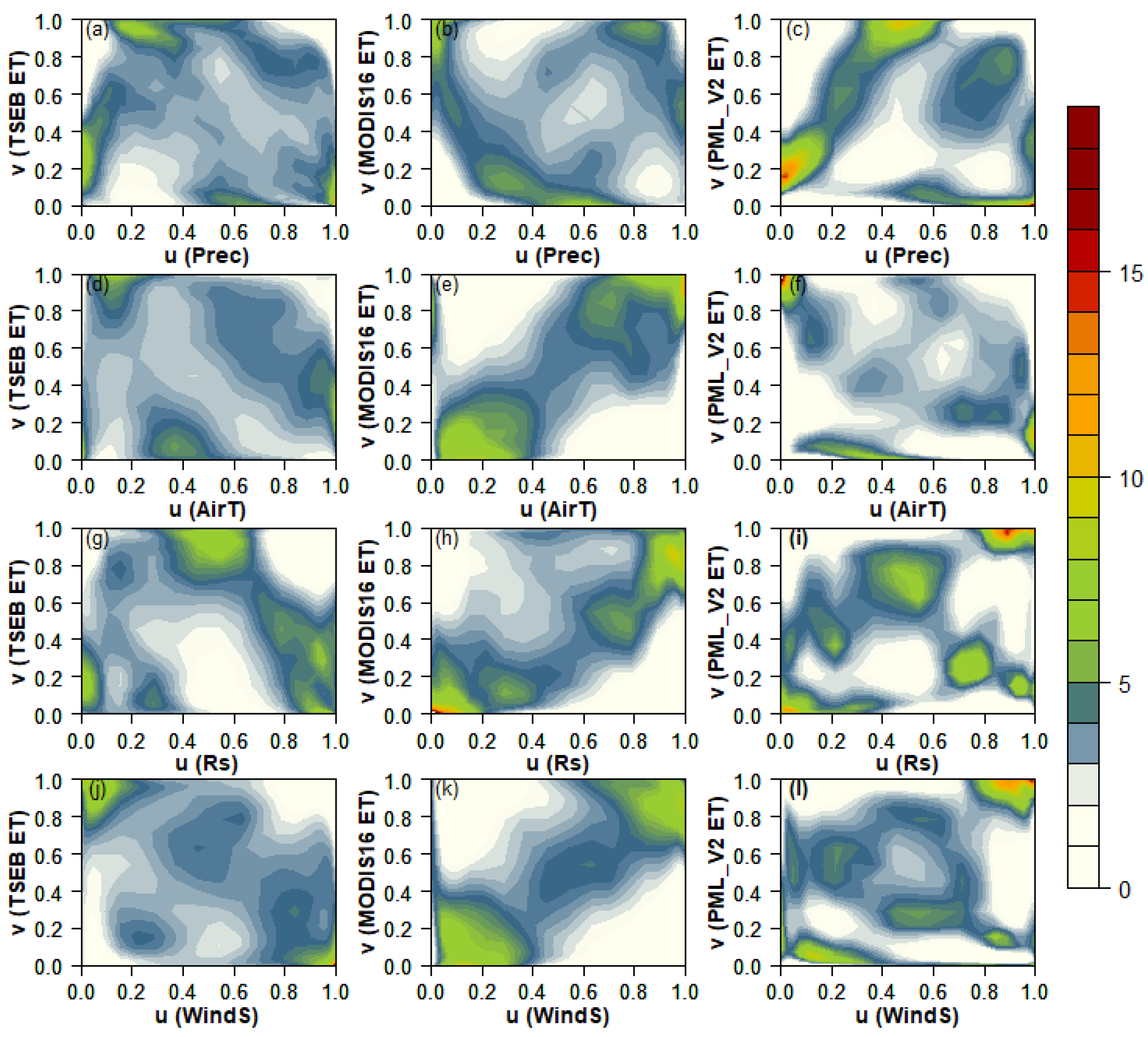
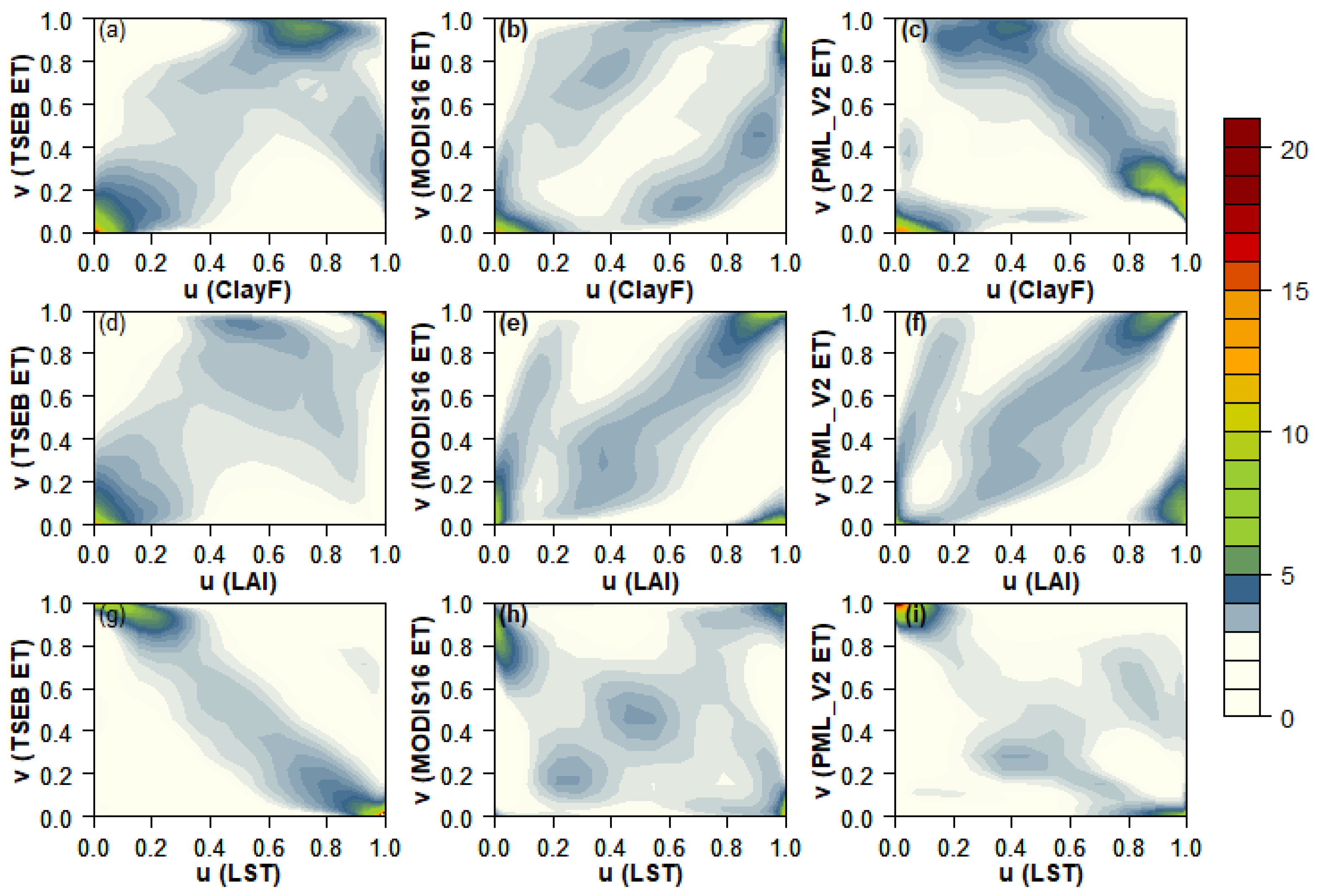
The empirical Copula densities of RS ET datasets and meteorological variables are illustrated in Figure A3. A nonlinear structure of the joint relationship for TSEB (Figure A3a), MODIS16 (Figure A3b), and PML_V2 (Figure A3c), in relation to Prec can be observed with multiple densities. In all cases, the highest densities are found neither in upper-tail nor lower-tail corners, but in different percentiles of ET distributions. This indicates a complex dependence structure exists between the MODIS-based RS ET datasets and Prec over Denmark with an energy-limited environment. Copula densities for MODIS16 against AirT are almost asymmetrical (Figure A3e). This implies that the highest density function is seen in the upper-right (lower-left) corner, where the extreme (very low) values are found indicating a positive correlation. In contrast, TSEB and PML_V2 show a nonlinear, negative dependence structures against AirT (Figure A3d,f). Additionally, Rs and WindS variables represent a very similar pattern against the three MODIS-based ET products. This means that, PML_V2 (Figure A3i,l) and especially MODIS16 (Figure A3h,k) indicate a positive correlation against Rs and WindS; however, the Copula densities between TSEB versus these variables are negative, in particular for WindS (Figure A3j).
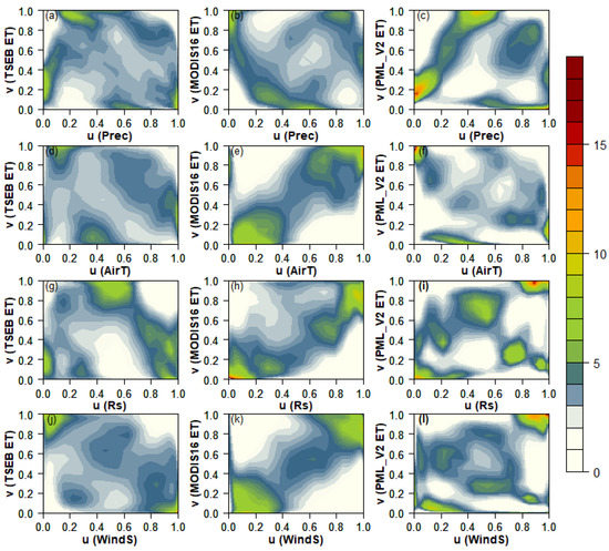
Figure A3.
Grid-based empirical Copula densities between the remote-sensing ET datasets (TSEB ET: left panels, MODIS16 ET: middle panels, and PML_V2 ET: right panels) and meteorological variables of precipitation Prec, air temperature AirT, global shortwave solar radiation Rs, and wind speed WindS. The sample size is 19,712 data tuples for all the variables. In all the panels (a–l), remote sensing ET (y-axis) are plotted against meteorological variables (x-axis).
As shown in Figure A4a–c, the empirical Copula density of MODIS-based ET against ClayF is asymmetrical (except for PML_V2) with the highest density in the lower-left corner (low values) for all three RS ET products. It indicates that they are strongly concordant in the lower ranks of the distribution; therefore, the three MODIS-based ET estimates (especially TSEB) are mainly affected by low values of ClayF over Denmark. The Copula density of TSEB (Figure A4d), MODIS16 (Figure A4e), and PML_V2 (Figure A4f) against LAI, unlike to ClayF, indicates a significant (positive) symmetric dependence structure with maximum densities in the lower-left and upper-right corners. This means that, highest correlation is found at the very low and extreme values. Amongst the land-surface/meteo-forcing variables applied, LST represents the most significant symmetrical dependence structure with TSEB (Figure A4g), meaning that the highest correlation is seen at lower-right and upper-left corners, indicating a strong negative correlation. However, the density function for MODIS16 and PML_V2 versus LST is mainly asymmetric with maximum dependency in the upper-left corner, as shown in Figure A4h,i. These dependencies are in accordance with the RS ET models for MODIS16, PML_V2, and TSEB, which all are driven by LAI, but only TSEB includes LST.
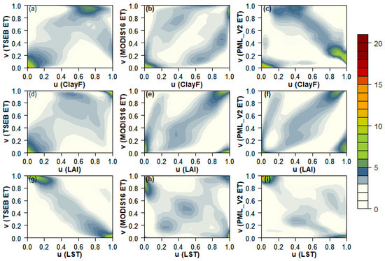
Figure A4.
Same as in Figure A3, but for the land-surface variables of clay fraction ClayF (top panels), leaf area index LAI (middle panels), and land surface temperature LST (bottom panels). In all the panels (a–i), remote sensing ET (y-axis) are plotted against land-surface variables (x-axis).
Figure A4.
Same as in Figure A3, but for the land-surface variables of clay fraction ClayF (top panels), leaf area index LAI (middle panels), and land surface temperature LST (bottom panels). In all the panels (a–i), remote sensing ET (y-axis) are plotted against land-surface variables (x-axis).
Appendix B.2. The Catchment-Based WB ET Dependence Structures
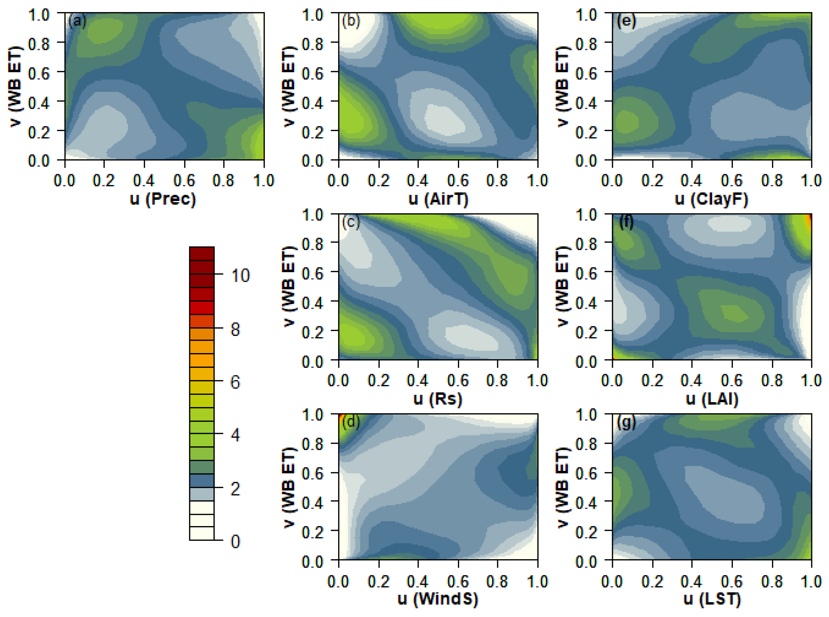
The empirical Copula densities of WB ET against land-surface and meteorological variables are illustrated in Figure A5. The density function for WB ET and Prec is negatively asymmetrical. This implies that the maximum dependency is seen in the lower-right tail, where the extreme (minimum) values of Prec (WB ET) are found; however, a second maximum can be also observed in the approx. upper-left corner (Figure A5a). As shown in Figure A5b,c, a nonlinear structure of the joint relationship for both AirT/Rs against WB ET is observed, with strongly varying densities in the different percentiles. The highest densities are mainly found for WB ET lower/higher values in the lower-left corners, whereas the upper-tails do not show a significant dependence structure in both AirT and Rs. This means that the highest WB ET values are not—or insignificantly affected by these variables. The distribution of WB ET against WindS is asymmetrical, with the highest density in the upper-left tail. It conveys that higher ranks of WB ET distribution are strongly concordant with the lowest WindS values, indicating a strong negative correlation. However, a weaker concordance is also observed in the lower—and middle range of values (Figure A5d).
The empirical Copula densities of WB ET against land-surface variables are also estimated. The density function of WB ET and ClayF is largely asymmetrical with the highest correlation in the upper-right tail, where the extreme values are found (Figure A5e). The Copula density between WB ET and LAI shows a strong symmetric dependence structure. The highest density is found for the upper-right tail, and a second maximum in the lower-left corner (Figure A5f). This conveys that they show the highest (positive) correlations for both the extreme—and low values, respectively. Nevertheless, an insignificant negative relationship can be also seen for the middle range of values. The dependence structure between WB ET versus LST indicates that the highest Copula densities are found in the maximum—and middle range of WB ET, which is corresponded to the middle range—and minimum values of LST, respectively. However, a third maximum density can be also observed for LST, indicating a negative correlation with WB ET (Figure A5g).
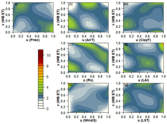
Figure A5.
Catchment-based empirical Copula densities between the surface water balance ET estimate and meteorological variables (left and middle panels) and land-surface variables (right panels). The datasets are the same as in Figure A3 and Figure A4. The sample size is 146 data tuples for all the variables. In all the panels (a–g), water balance ET (y-axis) are plotted against meteorological and land-surface variables (x-axis).
References
- Chahine, M.T. The hydrological cycle and its influence on climate. Nature 1992, 359, 373–380. [Google Scholar] [CrossRef]
- Oki, T.; Kanae, S. Global hydrological cycles and world water resources. Science 2006, 313, 1068–1072. [Google Scholar] [CrossRef]
- Sheffield, J.; Wood, E.F.; Munoz-Arriola, F. Long-term regional estimates of evapotranspiration for Mexico based on downscaled ISCCP data. J. Hydrometeorol. 2010, 11, 253–275. [Google Scholar] [CrossRef]
- Samain, B.; Simons, G.W.H.; Voogt, M.P.; Defloor, W.; Bink, N.J.; Pauwels, V.R.N. Consistency between hydrological model, large aperture scintillometer and remote sensing based evapotranspiration estimates for a heterogeneous catchment. Hydrol. Earth Syst. Sci. 2012, 16, 2095–2107. Available online: www.hydrol-earth-syst-sci.net/16/2095/2012/ (accessed on 1 July 2020). [CrossRef]
- Zhang, B.; Xia, Y.; Long, B.; Hobbins, M.; Zhao, X.; Hain, C.; Li, Y.; Anderson, M.C. Evaluation and comparison of multiple evapotranspiration data models over the contiguous United States: Implications for the next phase of NLDAS (NLDAS-Testbed) development. Agric. For. Meteorol. 2019, 280, 107810. [Google Scholar] [CrossRef]
- Xu, C.Y.; Singh, V.P. Evaluation of three complementary relationship evapotranspiration models by water balance approach to estimate actual regional evapotranspiration in different climatic regions. J. Hydrol. 2005, 308, 105–121. [Google Scholar] [CrossRef]
- Gao, Y.; Long, D. Intercomparison of remote sensing-based models for estimation of evapotranspiration and accuracy assessment based on SWAT. Hydrol. Process. 2008, 22, 4850–4869. [Google Scholar] [CrossRef]
- Peng, J.; Loew, A.; Chen, X.; Ma, Y.; Su, Z. Comparison of satellite-based evapotranspiration estimates over the Tibetan Plateau. Hydrol. Earth Syst. Sci. 2016, 20, 3167–3182. Available online: www.hydrol-earth-syst-sci.net/20/3167/2016/ (accessed on 1 July 2020). [CrossRef]
- Baldocchi, D.; Falge, E.; Gu, L.; Olson, R.; Hollinger, D.; Running, S.W.; Anthoni, P.; Bernhofer, C.; Davis, K.; Evans, R.; et al. FLUXNET: A new tool to study the temporal and spatial variability of ecosystem-scale carbon dioxide, water vapor, and energy flux densities. Bull. Am. Meteorol. Soc. 2001, 82, 2415–2434. [Google Scholar] [CrossRef]
- Wilson, K.B.; Hanson, P.J.; Mulholland, P.J.; Baldocchi, D.D.; Wullschleger, S.D. A comparison of methods for determining forest evapotranspiration and its components: Sap-flow, soil water budget, eddy covariance and catchment water balance. Agric. For. Meteorol. 2001, 106, 153–168. [Google Scholar] [CrossRef]
- Mauder, M.; Foken, T. Impact of post-field data processing on eddy covariance flux estimates and energy balance closure. Meteorol. Z. 2006, 15, 597–609. [Google Scholar] [CrossRef]
- Soltani, M.; Mauder, M.; Laux, P.; Kunstmann, H. Turbulent flux variability and energy balance closure in the TERENO prealpine observatory: A hydrometeorological data analysis. Theor. Appl. Climatol. 2017, 133, 937–956. [Google Scholar] [CrossRef]
- Ringgaard, R.; Herbst, M.; Friborg, T.; Schelde, K.; Thomsen, A.; Søgaard, H. Energy fluxes above three disparate surfaces in a temperate mesoscale coastal catchment. Vadose Zone J. 2011, 10, 54–66. [Google Scholar] [CrossRef][Green Version]
- Mendiguren, G.; Koch, K.; Stisen, S. Spatial pattern evaluation of a calibrated national hydrological model—A remote-sensing-based diagnostic approach. Hydrol. Earth Syst. Sci. 2017, 21, 5987–6005. [Google Scholar] [CrossRef]
- Milly, P.C.D.; Dunne, K.A. Trends in evaporation and surface cooling in the Mississippi River basin. Geophys. Res. Lett. 2001, 28, 1219–1222. [Google Scholar] [CrossRef]
- Walter, M.T.; Wilks, D.S.; Parlange, J.Y.; Schneider, R.L. Increasing evapotranspiration from the conterminous United States. J. Hydrometeorol. 2004, 5, 405–408. [Google Scholar] [CrossRef]
- Conradt, T.; Wechsung, F.; Bronstert, A. Three perceptions of the evapotranspiration landscape: Comparing spatial patterns from a distributed hydrological model, remotely sensed surface temperatures, and sub-basin water balances. Hydrol. Earth Syst. Sci. 2013, 17, 2947–2966. Available online: www.hydrol-earth-syst-sci.net/17/2947/2013/ (accessed on 10 April 2020). [CrossRef]
- Zeng, Z.; Wang, T.; Zhou, F.; Ciais, P.; Mao, J.; Shi, X.; Piao, S. A worldwide analysis of spatiotemporal changes in water balance-based evapotranspiration from 1982 to 2009. J. Geophys. Res. Atmos. 2014, 119, 1186–1202. [Google Scholar] [CrossRef]
- Han, E.; Crow, W.T.; Hain, C.R.; Anderson, M.C. On the use of a water balance to evaluate interannual terrestrial ET variability. J. Hydrometeorol. 2015, 16, 1102–1108. [Google Scholar] [CrossRef]
- Wang, S.; Huang, J.; Yang, D.; Pavlic, G.; Li, J. Long-term water budget imbalances and error sources for cold region drainage basins. Hydrol. Process. 2015, 29, 2125–2136. [Google Scholar] [CrossRef]
- Liu, W.; Wang, L.; Zhou, J.; Li, Y.; Sun, F.; Fu, G.; Li, X.; Sang, Y.F. A worldwide evaluation of basin-scale evapotranspiration estimates against the water balance method. J. Hydrol. 2016, 538, 82–95. [Google Scholar] [CrossRef]
- Mao, Y.; Wang, K. Comparison of evapotranspiration estimates based on the surface water balance, modified Penman-Monteith model, and reanalysis data sets for continental China. J. Geophys. Res. Atmos. 2017, 122, 3228–3244. [Google Scholar] [CrossRef]
- Dai, A.; Qian, T.; Trenberth, K.E.; Milliman, J.D. Changes in continental freshwater discharge from 1948 to 2004. J. Clim. 2009, 22, 2773–2792. [Google Scholar] [CrossRef]
- Wang, S.; McKenney, D.W.; Shang, J.; Li, J. A national-scale assessment of long-term water budget closures for Canada’s watersheds. J. Geophys. Res. Atmos. 2014, 119, 8712–8725. [Google Scholar] [CrossRef]
- Bouaziz, L.; Weerts, A.; Schellekens, J.; Sprokkereef, E.; Stam, J.; Savenije, H.; Hrachowitz, M. Redressing the balance: Quantifying net intercatchment groundwater flows. Hydrol. Earth Syst. Sci. 2018, 22, 6415–6434. [Google Scholar] [CrossRef]
- Danapour, M.; Højberg, A.L.; Jensen, K.H.; Stisen, S. Assessment of regional inter-basin groundwater flow using both simple and highly parameterized optimization schemes. Hydrogeol. J. 2019, 27, 1929–1947. [Google Scholar] [CrossRef]
- Genereux, D.P.; Jordan, M.T.; Carbonell, D. A paired-watershed budget study to quantify interbasin groundwater flow in a lowland rain forest, Costa Rica. Water Resour. Res. 2005, 41, W04011. [Google Scholar] [CrossRef]
- Frisbee, M.D.; Tysor, E.H.; Stewart-Maddox, N.S.; Tsinnajinnie, L.M.; Wilson, J.L.; Granger, D.E.; Newman, B.D. Is there a geomorphic expression of interbasin groundwater flow in watersheds? Interactions between interbasin groundwater flow, springs, streams, and geomorphology. Geophys. Res. Lett. 2016, 43, 1158–1165. [Google Scholar] [CrossRef]
- Friedl, M.A. Relationships among remotely sensed data, surface energy balance, and area-averaged fluxes over partially vegetated land surfaces. J. Appl. Meteorol. 1996, 35, 2091–2103. [Google Scholar] [CrossRef]
- Su, Z. The Surface Energy Balance System (SEBS) for estimation of turbulent heat fluxes. Hydrol. Earth Syst. Sci. 2002, 6, 85–100. [Google Scholar] [CrossRef]
- Wang, S.; Trishchenko, A.P.; Khlopenkov, K.V.; Davidson, A. Comparison of International Panel on Climate Change Fourth Assessment Report climate model simulations of surface albedo with satellite products over northern latitudes. J. Geophys. Res. 2006, 111, D21108. [Google Scholar] [CrossRef]
- Gowda, P.H.; Chávez, J.L.; Colaizzi, P.; Tolk, J. Remote sensing based energy balance algorithms for mapping ET: Current status and future challenges. Trans. ASABE 2007, 55, 1639–1644. [Google Scholar] [CrossRef]
- Zhang, Y.; Peña-Arancibia, J.; McVicar, T.; Chiew, F.H.S.; Vaze, J.; Liu, C.; Lu, X.; Zheng, H.; Wang, Y.; Liu, Y.Y.; et al. Multi-decadal trends in global terrestrial evapotranspiration and its components. Sci. Rep. 2016, 6, 19124. [Google Scholar] [CrossRef]
- Senay, G.B.; Leake, S.; Nagler, P.L.; Artan, G.; Dickinson, J.; Cordova, J.T.; Glenn, E.P. Estimating basin scale evapotranspiration (ET) by water balance and remote sensing methods. Hydrol. Process. 2011, 25, 4037–4049. [Google Scholar] [CrossRef]
- Allen, R.G.; Pereira, L.S.; Howell, T.A.; Jensen, M.E. Evapotranspiration information reporting: I. Factors governing measurement accuracy. Agric. Water Manag. 2011, 98, 899–920. [Google Scholar] [CrossRef]
- Stisen, S.; Sandholt, I.; Nørgaard, A.; Fensholt, R.; Høgh Jensen, K. Combining the triangle method with thermal inertia to estimate regional evapotranspiration—Applied to MSG-SEVIRI data in the Senegal River basin. Remote Sens. Environ. 2008, 112, 1242–1255. [Google Scholar] [CrossRef]
- Anderson, M.C.; Kustas, W.P.; Norman, J.M.; Hain, C.R.; Mecikalski, J.R.; Schultz, L.; González-Dugo, M.P.; Cammalleri, C.; d’Urso, G.; Pimstein, A.; et al. Mapping daily evapotranspiration at field to continental scales using geostationary and polar orbiting satellite imagery. Hydrol. Earth Syst. Sci. 2011, 15, 223. Available online: www.hydrol-earth-syst-sci.net/15/223/2011/ (accessed on 20 March 2020). [CrossRef]
- Guerschman, J.P.; Van Dijk, A.I.; Mattersdorf, G.; Beringer, J.; Hutley, L.B.; Leuning, R.; Pipunic, R.C.; Sherman, B.S. Scaling of potential evapotranspiration with MODIS data reproduces flux observations and catchment water balance observations across Australia. J. Hydrol. 2009, 369, 107–119. [Google Scholar] [CrossRef]
- Vinukollu, R.K.; Wood, E.F.; Ferguson, C.R.; Fisher, J.B. Global estimates of evapotranspiration for climate studies using multi-sensor remote sensing data: Evaluation of three process-based approaches. Remote Sens. Environ. 2011, 115, 801–823. [Google Scholar] [CrossRef]
- Mu, Q.; Zhao, M.; Running, S.W. Improvements to a MODIS global terrestrial evapotranspiration algorithm. Remote Sens. Environ. 2011, 115, 1781–1800. [Google Scholar] [CrossRef]
- Senay, G.B.; Bohms, S.; Singh, R.K.; Gowda, P.H.; Velpuri, N.M.; Alemu, H.; Verdin, J.P. Operational evapotranspiration mapping using remote sensing and weather datasets: A new parameterization for the SSEB approach. J. Am. Water Resour. Assoc. 2013, 49, 577–591. [Google Scholar] [CrossRef]
- Calsaverini, R.S.; Vicente, R. An information-theoretic approach to statistical dependence: Copula information. Europhys. Lett. 2009, 88, 3–12. [Google Scholar] [CrossRef]
- Bárdossy, A.; Pegram, G. Multiscale spatial recorrelation of RCM precipitation to produce unbiased climate change scenarios over large areas and small. Water Resour. Res. 2012, 48, 9502. [Google Scholar] [CrossRef]
- Soltani, M.; Laux, P.; Mauder, M.; Kunstmann, H. Spatiotemporal variability and empirical Copula-based dependence structure of modelled and observed coupled water and energy fluxes. Hydrol. Res. 2018, 49, 1396–1416. [Google Scholar] [CrossRef]
- Bárdossy, A. Copula-based statistical models for groundwater quality parameters. Water Resour. Res. 2006, 42, W11416.1–W11416.12. [Google Scholar]
- Sugimoto, T.; Bárdossy, A.; Pegram, G.S.; Cullmann, J. Investigation of hydrological time series using copulas for detecting catchment characteristics and anthropogenic impacts. Hydrol. Earth Syst. Sci. 2016, 20, 2705–2720. [Google Scholar] [CrossRef]
- Li, T.; Guo, S.; Liu, Z.; Xiong, L.; Yin, J. Bivariate design flood quantile selection using copulas. Hydrol. Res. 2016, 48, 997–1013. [Google Scholar] [CrossRef]
- Balistrocchi, M.; Bacchi, B. Derivation of flood frequency curves through a bivariate rainfall distribution based on copula functions: Application to an urban catchment in northern Italy’s climate. Hydrol. Res. 2017, 48, 749–762. [Google Scholar] [CrossRef]
- Laux, P.; Wagner, S.; Wagner, A.; Jacobeit, J.; Bárdossy, A.; Kunstmann, H. Modelling daily precipitation features in the Volta Basin of West Africa. Int. J. Climatol. 2009, 29, 937–954. [Google Scholar] [CrossRef]
- Zhang, Q.; Li, J.F.; Singh, V.P.; Xu, C.Y. Copula-based spatio-temporal patterns of precipitation extremes in China. Int. J. Climatol. 2013, 33, 1140–1152. [Google Scholar] [CrossRef]
- Mao, G.; Vogl, S.; Laux, P.; Wagner, S.; Kunstmann, H. Stochastic bias correction of dynamically downscaled precipitation fields for Germany through Copula-based integration of gridded observation data. Hydrol. Earth Syst. Sci. 2015, 19, 1787–1806. Available online: www.hydrol-earth-syst-sci.net/19/1787/2015/ (accessed on 1 July 2020). [CrossRef]
- Laux, P.; Vogl, S.; Qiu, W.; Knoche, H.R.; Kunstmann, H. Copula-based statistical refinement of precipitation in RCM simulations over complex terrain. Hydrol. Earth Syst. Sci. 2011, 15, 2401–2419. Available online: www.hydrol-earth-syst-sci.net/15/2401/2011/ (accessed on 20 May 2020). [CrossRef]
- Schneider, R.; Henriksen, H.J.; Stisen, S. A Robust Objective Function for Calibration of Groundwater Models in Light of Deficiencies of Model Structure and Observations. Available online: https://hess.copernicus.org/preprints/hess-2019-685/ (accessed on 20 May 2020).
- Mao, Y.; Wang, K.; Liu, X.; Liu, C. Water storage in reservoirs built from 1997 to 2014 significantly altered the calculated evapotranspiration trends over China. J. Geophys. Res. Atmos. 2016, 121, 10097–10112. [Google Scholar] [CrossRef]
- Velpuri, N.M.; Senay, G.B.; Singh, R.K.; Bohms, S.; Verdin, J.P. A comprehensive evaluation of two MODIS evapotranspiration products over the conterminous United States: Using point and gridded FLUXNET and water balance ET. Remote Sens. Environ. 2013, 139, 35–49. [Google Scholar] [CrossRef]
- Zhang, Y.; Kong, D.; Gan, R.; Chiew, F.H.S.; McVicar, T.R.; Zhang, Q.; Yang, Y. Coupled estimation of 500m and 8-day resolution global evapotranspiration and gross primary production in 2002–2017. Remote Sens. Environ. 2019, 222, 165–182. [Google Scholar] [CrossRef]
- Norman, J.M.; Kustas, W.P.; Humes, K.S. Source approach for estimating soil and vegetation energy fluxes in observations of directional radiometric surface temperature. Agric. For. Meteorol. 1995, 77, 263–293. [Google Scholar] [CrossRef]
- Vejen, F.; Vilic, K.; Jensen, H. Korrigeret Nedbør 1989–2010, 2011–2012 and 2013, DMI Technical Report 14-13; Technical Report; Danish Meteorological Institute: Copenhagen, Denmark, 2014. [Google Scholar]
- Miralles, D.G.; Holmes, T.R.H.; De Jeu, R.A.M.; Gash, J.H.; Meesters, A.G.C.A.; Dolman, A.J. Global land-surface evaporation estimated from satellite-based observations. Hydrol. Earth Syst. Sci. 2011, 15, 453–469. Available online: www.hydrol-earth-syst-sci.net/15/453/2011/ (accessed on 1 April 2020). [CrossRef]
- Ghilain, N.; Arboleda, A.; Gellens-Meulenberghs, F. Evapotranspiration modelling at large scale using near-real time MSG SEVIRI derived data. Hydrol. Earth Syst. Sci. 2011, 15, 771–786. Available online: www.hydrol-earth-syst-sci.net/15/771/2011/ (accessed on 25 September 2020). [CrossRef]
- Mu, Q.; Heinsch, F.A.; Zhao, M.; Running, S.W. Development of a global evapotranspiration algorithm based on MODIS and global meteorology data. Remote Sens. Environ. 2007, 111, 519–536. [Google Scholar] [CrossRef]
- Monteith, J.L. Evaporation and the environment. Symp. Soc. Exp. Biol. 1965, 19, 205–233. [Google Scholar]
- Kalma, J.D.; McVicar, R.; McCabe, F. Estimating land surface evaporation: A review of methods using remotely sensed surface temperature data. Surv. Geophys. 2008, 29, 421–469. [Google Scholar] [CrossRef]
- Henriksen, H.J.; Troldborg, L.; Nyegaard, P.; Sonnenborg, T.O.; Refsgaard, J.C.; Madsen, B. Methodology for construction, calibration and validation of a national hydrological model for Denmark. J. Hydrol. 2003, 280, 52–71. [Google Scholar] [CrossRef]
- Stisen, S.; Højberg, A.L.; Troldborg, L.; Refsgaard, J.C.; Christensen, B.S.B.; Olsen, M.; Henriksen, H.J. On the importance of appropriate precipitation gauge catch correction for hydrological modelling at mid to high latitudes. Hydrol. Earth Syst. Sci. 2012, 16, 4157–4176. Available online: www.hydrol-earth-syst-sci.net/16/4157/2012/ (accessed on 1 February 2020). [CrossRef]
- Højberg, A.L.; Troldborg, L.; Stisen, S.; Christensen, B.B.S.; Henriksen, H.J. Stakeholder driven update and improvement of a national water resources model. Environ. Model. Softw. 2013, 40, 202–213. [Google Scholar] [CrossRef]
- Abbott, M.B.; Bathurst, J.C.; Cunge, J.A.; O’Connell, P.E.; Rasmussen, J. An introduction to the European Hydrological System —Systeme Hydrologique Europeen, “SHE”, 1: History and philosophy of a physically based, distributed modelling system. J. Hydrol. 1986, 87, 45–59. [Google Scholar] [CrossRef]
- Graham, D.N.; Butts, M.B. Flexible, integrated watershed modelling with MIKE SHE. In Watershed Models; Taylor and Francis Group: Boca Raton, FL, USA, 2005; pp. 245–272. [Google Scholar]
- Stisen, S.; McCabe, M.F.; Refsgaard, J.C.; Lerer, S.; Butts, M.B. Model parameter analysis using remotely sensed pattern information in a multi-constraint framework. J. Hydrol. 2011, 409, 337–349. [Google Scholar] [CrossRef]
- Gupta, H.V.; Kling, H.; Yilmaz, K.K.; Martinez, G.F. Decomposition of the mean squared error and NSE performance criteria: Implications for improving hydrological modelling. J. Hydrol. 2009, 377, 80–91. [Google Scholar] [CrossRef]
- Stisen, S.; Ondracek, M.; Troldborg, L.; Schneider, R.; Jon van Til, M. National Vandressource Model Modelopstilling og Kalibrering af DK-Model 2019 (In Danish). Geological Survey of Denmark and Greenland—Report. 2019. Available online: http://dk.vandmodel.dk/media/21560/geusrapport2019_31_dkmodel2019_web-1.pdf (accessed on 1 February 2020).
- Sklar, A. Fonctions de Repartition á n Dimensions et Leurs Marges; Publications de l’Institut de statistique de l’Université de Paris: Paris, France, 1959; Volume 8, pp. 229–231. [Google Scholar]
- Salvadori, G.; Michele, C.D.; Kottegoda, N.; Rosso, R. Extremes in Nature: An Approach Using Copulas. In Water Science and Technology Library; Springer: Berlin, Germany, 2007; Volume 56. [Google Scholar]
- Serinaldi, F. A multisite daily rainfall generator driven by bivariate copula-based mixed distrbutions. J. Geophys. Res. 2009, 114, D10103. [Google Scholar] [CrossRef]
- Nelsen, R. An Introduction to Copulas; Springer: New York, NY, USA, 1999. [Google Scholar]
- Genest, C.; Favre, A.C. Everything you always wanted to know about copula modeling but were afraid to ask. J. Hydrol. Eng. 2007, 12, 347–368. [Google Scholar] [CrossRef]
- Nagler, T. kdecopula: An R Package for the Kernel Estimation of Bivariate Copula Densities. J. Stat. Softw. 2018, 84, 1–22. [Google Scholar] [CrossRef]
- Deheuvels, P. La fonction de dépendance empirique et ses propriétés: Un test non paramétrique d’indépendance, Académie Royale de Belgique. Bulletin de la Classe des. Sciences 1979, 65, 274–292. [Google Scholar]
- Abdi, H.; Williams, L.J. Principal component analysis. Wires Comput. Stat. 2010, 2, 433–459. [Google Scholar] [CrossRef]
- Jolliffe, I. Principal Component Analysis, 2nd ed.; Springer: Berlin, Germany, 2002. [Google Scholar] [CrossRef]
- Naik, G.R. Advances in Principal Component Analysis: Research and Development; Springer: Berlin/Heidelberg, Germany, 2018. [Google Scholar] [CrossRef]
- Cappelen, J.; Kern-Hansen, C.; Vaarby Laursen, E.; Viskum Jørgensen, P.; Vraa Jørgensen, B. DMI Report 19-02: Denmark-DMI Historical Climate Data Collection 1768–2018; Danish Meteorological Institute: Copenhagen, Denmark, 2018; Available online: https://www.dmi.dk/publikationer/ (accessed on 5 August 2020).
- Poulsen, J.B. Stream Flow–Its Estimation, Uncertainty and Interaction with Groundwater and Floodplains; Aarhus University: Aarhus, Denmark, 2013. [Google Scholar]
- Liou, Y.A.; Kar, S.K. Evapotranspiration estimation with remote sensing and various surface energy balance algorithms—A review. Energies 2014, 7, 2821–2849. [Google Scholar] [CrossRef]
- Miralles, D.G.; Jiménez, C.; Jung, M.; Miche, D.; Ershadi, A.; McCabe, M.F.; Hirschi, M.; Martens, B.; Dolman, A.J.; Fisher, J.B.; et al. The WACMOS-ET project—Part 2: Evaluation of global land evaporation data sets. Hydrol. Earth Syst. Sci. 2016, 20, 823–842. Available online: www.hydrol-earth-syst-sci.net/20/823/2016/ (accessed on 10 June 2020). [CrossRef]
- McCabe, M.F.; Wood, E.F. Scale influences on the remote estimation of evapotranspiration using multiple satellite sensors. Remote Sens. Environ. 2006, 105, 271–285. [Google Scholar] [CrossRef]
Publisher’s Note: MDPI stays neutral with regard to jurisdictional claims in published maps and institutional affiliations. |
© 2021 by the authors. Licensee MDPI, Basel, Switzerland. This article is an open access article distributed under the terms and conditions of the Creative Commons Attribution (CC BY) license (http://creativecommons.org/licenses/by/4.0/).

