Article

Using Satellite Gravity and Hydrological Data to Estimate Changes in Evapotranspiration Induced by Water Storage Fluctuations in the Three Gorges Reservoir of China

Hubei Subsurface Multi-Scale Imaging Key Laboratory, Institute of Geophysics and Geomatics, China University of Geosciences, Wuhan 430074, China
*
Author to whom correspondence should be addressed.
Remote Sens. 2020, 12(13), 2143; https://doi.org/10.3390/rs12132143
Submission received: 15 May 2020 / Revised: 26 June 2020 / Accepted: 2 July 2020 / Published: 3 July 2020

Abstract

:
The change in water storage driven by the Three Gorges Project directly affects the terrestrial water migration and redistribution in the Yangtze River Basin (YRB). As a result, a new water balance is established and regional evapotranspiration (ET) fluctuates in the process. In this paper, data from multiple-sources including from the Gravity Recovery and Climate Experiment (GRACE) satellite, land surface models (LSMs), remote sensing, and in-situ observations were used to monitor the temporal and spatial evolution of terrestrial water and estimate changes in ET in the Three Gorges Reservoir (TGR) from 2002 to 2016. Our results showed that GRACE data scaled using the scale factor method significantly improved the signal amplitude and highlighted its spatial differences in the TGR area. Combining GRACE with surface hydrological observations, ET in the TGR area was estimated to have overall change characteristics highly consistent with results from the MOD16 Moderate Resolution Imaging Spectroradiometer (MODIS), and the uncertainties of monthly ET are mainly from TWS changes derived by GRACE uncertainties such as measurement errors and leakage errors. During our study period, the cyclical ET was mainly driven by climate precipitation but short-term (monthly) ET in the TGR area was also directly affected by human-driven water storage. For example, rising water levels in the three water storage stages (2003, 2006, and 2008) caused an abnormal increase in regional ET (up to 22.4 cm/month, 19.2 cm/month and 29.5 cm/month, respectively). Usually, high precipitation will cause increase in ET but the high precipitation during the water release periods (spring and summer) did not have a significant impact on the increased ET due to the water level in the TGR having decreased 30 m in this stage. Our results also indicate that the short-term fluctuations in flooded area and storage capacity of the TGR, i.e., the man-made mass changes in the main branch and tributaries of the Yangtze River, were the main factors that influenced the ET. This further illustrated that a quantitative estimation of changes in the ET in the TGR allows for a deeper understanding of the water balance in the regional land water cycle process as driven by both climate and human factors.

Graphical Abstract

1. Introduction

Terrestrial water storage (TWS) is the main carrier by which mass circulation, migration, and exchange is accomplished between the earth’s terrestrial, oceanic, and atmospheric systems [1]. TWS also plays a vital role in allowing for agricultural irrigation, industrial, and domestic water supplies, and are essential for human survival and development. Anthropogenic influences in the global water cycle have become increasingly prominent and cannot be excluded from analyses of current and future hydrological systems [2]. Monitoring how TWS changes under the background of human activities allows an understanding of the impacts of global and regional climate change through the lens of hydrological events such as droughts, floods, and changes in groundwater supply [3]. TWS as the main carrier in the terrestrial water cycle, in-depth analysis of the water cycle will have a deeper understanding of TWS. In addition, analysis of the temporal and spatial evolution of regional terrestrial water cycles can provide long-term, reasonable guidelines for water resources development and management [4]. Over the past few decades, climate change and human activities have exacerbated the abnormal hydrological cycle, which has important implications for ecosystem services and feedback to regional and global climates [5]. As a linking mechanism between the land surface and the atmosphere [6], evaporation (E) and evapotranspiration (ET) are fundamental components of the water balance and major variables for analyzing the changes of the water level and volume in a lake [7]. Long-term changes in ET have important implications for regional climate change and water cycle studies. Thus, study on the spatio-temporal changes of ET is essential to accurately estimate the global or regional water budget and to further figure out the hydrological interaction between Earth’s surface (land, rivers and lakes) and atmosphere.
The Three Gorges Project is an anthropogenic factor that affects terrestrial water migration and redistribution. It is located in the middle and upper reaches of the Yangtze River and was completed on 20 May 2006. And the storage capacity can reach 39.3 billion cubic meters. While the Three Gorges Project has generated high levels of concern from around the world, it offers communities multiple benefits such as flood control, power generation, shipping, and water resources regulation [8]. However, since the launch of the project, disputes over the ecological, climatic, and environmental impacts of the dam have not subsided. The Three Gorges Reservoir (TGR) area was largely defined based on the climatic, geologic, and geomorphologic characteristics of the river basin. While the TGR brings economic benefits [9], it also changes the processes of terrestrial water circulation. For example, long-term water interception and storage by dams will affect the redistribution of terrestrial water [10], and the artificial lake formed will cause regional ET to fluctuate. The ET is dependent on surface heat balance and water balance and is the component of the water cycle that is most directly affected by land use and climate change. Quantitative estimation of the ET in the TGR area will provide an understanding of the state of the water balance in the Three Gorges region and can help with analysis of the regional terrestrial water cycle process and understanding the degree to which it is driven by climatic and human factors.
Tower-based eddy covariance and pan evaporation equipment are generally used to observe ET, but such methods are limited by the observation conditions at the site. The observed pan evaporation data is discontinuous in the space-time domain and is difficult to measure at the regional scale. In addition, the pan evaporation is a measurement that combines or integrates the effects of several climate elements (i.e., temperature, humidity, rainfall, drought dispersion, solar radiation, and wind). Usually, pan evaporation is used to estimate the evaporation from lakes but those data cannot fully represent the true-ET from the natural climate change, for example, the ET from a natural body of water is a lower rate than observed pan data because the light penetration in natural bodies of water will decrease as depth, while light penetration in a pan is essentially uniform and the pan metal sides that get hot with the sun [11,12,13,14]. At the basin scale, net runoff is equal to total precipitation minus ET. Thus, ET can be estimated via the basin water balance, although this method generally ignores the impact of changes in terrestrial water reserves [15,16]. Since the Three Gorges Project was established in 1994 and experimental storage of 175 m (the highest design water level) started in 2008, there have been a series of studies on the significant changes in hydrological cycles that have occurred and their potential impact on climate and environmental variables using different data, methods, and scales [17,18,19,20]. However, changes in ET in the TGR and surrounding areas have rarely been studied due to the coarse spatial-temporal resolution and limited accuracy of the observations.
The launch of the Gravity Recovery and Climate Experiment (GRACE) satellites in 2002 provides an important source of data for more accurate terrestrial water flux [21,22] and effective ET estimation. For example, Rodell et al. [23] first discussed the method of estimating ET using GRACE and other observed data at the basin scale. Long et al. [24] estimated the uncertainty in ET based on the GRACE water balance equation at the basin scale. Li et al. [25] improved the method for estimating the ET water balance equation based on GRACE data and estimated the changes in ET in the Yangtze River Basin (YRB) from 2003 to 2013. The combination of surface and satellite, hydrometeorological, and geophysical or geodetic survey data has gradually become the main method for monitoring TWS and other types of surface hydrological process from a local to large scale. This combination of methods also shows great potential in studying ET in a single region. However, truncating and filtering of GRACE data reduces the signal amplitude and significantly reduces the spatial resolution, and thus provides a band-limited representation of near-surface mass changes. This is particularly problematic when studying mass changes in rivers and lakes because these mass changes tend to be concentrated in fairly narrow or smaller radius disc zones.
In previous GRACE-based studies, such small-scale phenomena have been studied with special methods depending on signal source characteristics. Several of these approaches employed corrections to restore the signal loss due to filtering, e.g., the additive method [26], the multiplicative method [27], the scaling factor method [28], and the data-driven method [29]. But these methods still depend on model assumptions and size of the study area. In this work, we both diagnose scaled GRACE solution and describe an approach to estimate ET in TGR. GRACE satellite gravity data, hydrological model results, and in-situ observations were used to estimate small-scale TWS in the TGR, we extracted 11 grids of scaled GRACE data, each grid with a resolution of 0.5°. The main processing flow is that the scaling factor was calculated basing on modeled TWS time series from optimal Land Surface Model (LSM), which was evaluated by in-situ observation. Then, based on the theory of watershed water balance, the temporal and spatial characteristics of total TWS, regional precipitation, and runoff were combined to extract the change in ET from 2002 to 2016 that was driven by the Three Gorges Project. This research provides evaluative data and references that can help better define the inter-relationship between the water storage induced by man-made projects and different environmental responses. Furthermore, the ET is significantly observable by GRACE data that could be good to consider assimilating the GRACE into the Hydrological model to update their ET estimates.

2. Study Area and Datasets

2.1. Three Gorges Reservoir Area

The total area of the YRB is 1.8 × 10⁶ km2, accounting for 18.8% of China’s total land area. The Yangtze River is more than 6300 km long and has many tributaries. The whole river basin is divided into 11 sub-basin systems, namely: four major river systems, three major north shore river systems, and four major south shore water systems. The YRB is China’s main agricultural production area, and more than 80% of the land area is suitable for agriculture and human habitation. In addition, the region contains about one fifth of the total lake area in China. The presence of irrigation systems and artificial reservoirs in the YRB has meant that previous works concentrated on studying the terrestrial water balance of the entire river basin and how climate and anthropogenic activities affected the balance [30,31,32,33,34].
The TGR is located in the middle and upper reaches of the Yangtze River (Figure 1) with a total area of 5.6 × 10⁴ km2. The upstream boundary is 106.58°E and the downstream boundary is 111.14°E. The Three Gorges Dam (TGD) is located in Sandouping Town, Yichang City, Hubei Province (i.e., 110.00°E, 30.82°N). The total storage capacity of the TGR reaches 39.3 km3 and the flood prevention storage capacity is 22.15 km3, reservoir flood regulation can reduce peak flood flow by 27,000 m3/s~33,000 m3/s, and the highest water level in the TGR can reach 175 m when water is stored. The reservoir can effectively control floods in the upper reaches of the Yangtze River, making it the most significant water conservancy project in the world. Existing research related to the TGR mainly includes: (1) monitoring seasonal and long-term changes in water storage based on GRACE data [35,36,37], and; (2) speculation on potential groundwater infiltration by combining GRACE data, hydrological models, and surface observations [8]. Those previous studies mainly studied the variation characteristics of TWS and its components, and did not discuss the water balance in the area in depth, such as ET, etc. Our study uses GRACE gravity satellite data, results from hydrological models, and surface observations to address issues in climate and TGR-driven TWS change and the resulting response in ET.

2.2. GRACE-Drived TWS Data

The GRACE RL06 spherical harmonic coefficient solution provided by CSR was used (Center for Space Research, University of Texas at Austin, USA), with an order from 2 to 96 and a time span from March 2002 to August 2016. The specific official processing information of this data can be referred to http://icgem.gfz-potsdam.de/GRACE_CSR_L2_Processing_Standards_Document_for_RL06.pdf. The satellite laser ranging coefficient was used to replace the C20 (degree 2 and order 0) coefficient, because of the insensitivity of the GRACE satellite orbit to the C20 coefficient and large uncertainty in its value [38,39]. The first-order coefficient term was corrected using the coefficient (geocentric) provided by Swenson et al. [40]. The results of Glacial Isostatic Adjustment (GIA, this model was calculated using the finite element method combined with the ICE-5G glacier ablation model and the VM2 viscosity profile earth model) given by A et al. [41] were used to correct the GIA effect from GRACE data. Measurements from GRACE are affected by the orbit error of the satellite and the truncation error of the spherical harmonic coefficient. To address this, a P4M6 decorrelation processing method was performed [42], followed by Gaussian filter processing with a correlation radius of 500 km [43].

2.3. Land Surface Models (LSMs)

The outputs of three LSMs were used in this study, during the post-processing of GRACE data, signal ‘leakage’ is caused by filtering such as signal reduction, bias, and signal leakage around the target area, which leads to GRACE underestimating or overestimating the true change of TWS [43,44]. In view of this, some studies use different methods to calculate the grid scaling factors of global and basin to restore the damage and deviation signals from GRACE [9,26,28,45]. In this study, the scale factor method was used based on LSMs to recover the “leakage” signal estimated by GRACE in the study area [9,28]. For example, the scale factor was derived using a least square fit between spatially averaged filtered and unfiltered modeled TWS anomaly time series. The three most commonly used LSMs, including GLDAS (Global Land Data Assimilation System) [46], WGHM (Water Global Hydrological Model) and CLM4.5 (Community Land Model 4.5) were used in the analysis [47,48]. The process method is shown in Section 3.1.
GLDAS is a global (excluding Greenland and Antarctica) high-resolution LSM established by the NASA (National Aeronautics and Space Administration) Goddard Space Flight Center and the National Centers of Environmental Prediction. It establishes a constrained model through land surface modeling and data assimilation techniques to provide optimized near-real-time information on land surface changes. The input data used by the GLDAS model includes the results of precipitation analysis, solar radiation, surface pressure, and humidity. The GLDAS forcing precipitation data are extracted from the National Oceanic and Atmospheric Administration (NOAA) and Climate Prediction Center (CPC) Merged Analysis of Precipitation (CMAP) [49], GLDAS simulates TWS as the summation of soil moistures, snow, and canopy storages through four main land surface models, CLM, Mosaic, Noah, and VIC. In this study, the Noah model was used with a spatial resolution of 1° × 1° and a time interval of one month.
WGHM is a global water analysis and prediction model provided by Goethe University Frankfurt, Germany with a spatial resolution of 0.5° × 0.5° and a time interval of one month. The WGHM is forced by a combination of a Global Precipitation Climatology Centre monthly precipitation data sets from 1901 till present, which are calculated from global station data in 1° × 1° global grids [50]. WGHM not only calculates the long-term average water resources of various countries or river basins, but also calibrates them using measurements. At the same time, all components of terrestrial water reserves except glaciers are also simulated, including changes in soil water, runoff, groundwater recharge, surface snow, and surface water reserves (such as vegetation canopy water, rivers, lakes, reservoirs, and wetlands).
CLM is a public LSM developed by the National Center for Atmospheric Research. CLM is one of the most comprehensive and widely used LSMs. It covers four sub-modules: biogeophysics, the hydrological cycle, biogeochemistry, and dynamic vegetation. CLM simulates the distribution of atmospheric mass and energy, the redistribution of mass and energy on land surfaces, and the output of fresh water and heat to the ocean. In order to realistically simulate these interactions, the CLM data includes terrestrial hydrological components, such as precipitation interception and infiltration by the canopy, evolution of surface water, groundwater, snow, and soil moisture, and evaporation and transpiration of soil and vegetation. CLM4.5 is forced with atmospheric conditions for the period 1850–2010 extracted from the Climate Research Unit, National Centers for Environmental Prediction (CRUNCEP) datasets (http://dods.extra.cea.fr/data/p529viov/cruncep/). Here, we use CLM4.5 with a spatial resolution of 1.25° × 0.9375° and a time interval of one month.

2.4. In-Situ Hydrological Observations

Specific comparative analysis of the differences in the output components of different LSMs were conducted based on the measured data (e.g., soil moisture and groundwater) from ground stations. The results were used to test the performance of LSM assimilation data in describing the TWS of the YRB, then the optimal LSM suitable for the study area was selected based on the performance. The in-situ measured groundwater and soil moisture data were from the China Meteorological Data Sharing Service System (CMDSSS, available at http://data.cma.cn/data/cdcindex.html). The groundwater data was observations from 136 wells evenly distributed in the YRB spanning January 2005 to December 2013 at a time resolution of one month. The soil moisture data was from 122 meteorological stations evenly distributed in the YRB spanning January 2002 to December 2014 at a time resolution of one month. The average value was deducted from the measured data for a similar period as GRACE. The process method is shown in Section 3.2.
To estimate ET based on watershed water balance methods, precipitation and runoff data should be subtracted from TWS changes. The precipitation data for this study were derived from a gridded data set of China’s daily precipitation value at a 0.5° × 0.5° scale also provided by the CMDSSS. This data set is based on the latest compiled precipitation data from surface high-density stations across China (2,472 national meteorological observatories) compiled by the China National Meteorological Information Center. The thin plate spline method in the ANUSPLIN software (https://fennerschool.anu.edu.au/research/products/anusplin) was used to perform spatial interpolation and create a dataset from 1961 to the present. Net runoff data came from the real-time outflow and inflow of the Three Gorges and Gezhouba dam provided by the data center of the Three Gorges Corporation. The process method is shown in Section 3.3.

2.5. MODIS-MOD16 ET Data

This study, surface ET data (MOD16) from the MODIS (Moderate Resolution Imaging Spectroradiometer) product was used to evaluate the estimated ET results derived from GRACE data. The ET from remote sensing data was based on the observations from MODIS sensors on the Aqua and Terra satellites, and the model algorithm was based on the Penman-Monteith remote sensing model [51], which used daily meteorological reanalysis data and MODIS remote sensing vegetation dynamic data as input. The final product is released by the NASA, with data coverage of 1.0903 × 10⁶ km2 of vegetated area. MOD16 data products include terrestrial ecosystem ET, latent heat flux, potential terrestrial ecosystem ET, and potential latent heat flux data. The spatial resolution is 500 m, and the time resolution differs with the product. MOD16A2 products have a time resolution of eight days, MOD16A3 products have a time resolution of a year, and MOD16A2G/A3GF are year-end filling data products. Here, MOD16A2-ET data products were selected for study.

3. Data Processing Methods

3.1. Post-Processing Method for Grace Data

The surface density change can be expanded in the spherical harmonic field as [43]:
σ ( θ , λ ) = a ρ E 3 l = 0 m = 0 l P ˜ l m ( cos θ ) 2 l + 1 1 + k l [ Δ C l m cos ( m λ ) + Δ S l m sin ( m λ ) ]
where ρ E is the average density of the earth (=5517 kg/m3); k l is the load love number at degree l, and a is the average radius of earth at the equator (=6371 km); P ˜ l m is the fully normalized associated Legendre polynomials of degree l and order m.
The surface mass change is usually regarded as the change in terrestrial water and can be represented in terms of the EWH (equivalent water height) Δ σ ρ w , where ρ ω is the density of water (=1000 kg/m3). Most of the monthly changes in the satellite gravity observations in this study area were caused by changes in the water storage capacity of TGR and other earth surface processes (such as the atmospheric and terrestrial water cycles). Usually, the range of these signals varies on a scale of centimeters, which is much smaller than the radius of the earth or the horizontal scale in kilometers. However, GRACE inversion results inevitably include the gravity change caused by the mass redistribution of the solid earth. In these cases, the interpretation of the change in gravity based on the ‘EWH’ is incorrect, but water-related mass changes can instead be isolated by removing solid earth effects. In this study, the solid tide was subtracted from the RL06 model data and the GIA effect was subtracted from the post-processing.
After inversion and post-processing of GRACE data, the EWH change in the TGR area was obtained from 2002 to 2016 (Figure 2). This was close to the trend in total terrestrial water in the TGR area from 2002 to 2010 obtained by Wang et al. [8] using GRACE data and surface observation data. The overall terrestrial water reserves in TGR showed a long-term growth trend, which was consistent with the three water storage stages of the TGD (135 m in 2003, 156 m in 2006, and 175 m in 2008), while the short-term trend showed more obvious seasonal fluctuations. The overall terrestrial water change in the TGR area is affected by climatic and human factors and is manifested through seasonal climate changes and reservoir capacity adjustment of the TGD.
The process by which the GRACE signal ‘leakage’ was recovered is shown in Figure 3. First, the selected hydrological model was processed with the same post-processing as the GRACE data [9], e.g., the LSMs were transformed from the spatial domain to the spherical harmonic domain (truncated to Lmax = 96) and Gaussian filtering with a 500 km radius was applied. Then, the scaling factor was calculated by the least squares fit between the filtered and unfiltered modeled TWS time series.
By multiplying the global scale factor grid with our equivalent water-height grid, the restored grid S was obtained. To obtain the EWH value of the study area, the basin kernel function is defined as:
υ ( θ , λ ) = { 0 , outside   the   area 1 × cos θ , within   the   area
The average EWH, H, of the study area can be expressed as:
H = 1 Ω i = 1 n S ( θ , λ ) × υ ( θ , λ )
where S is the EWH, n is the number of grid points, and Ω is the sum of the cosine values of the latitude of the grid points in the study area.

3.2. Selection of LSM Based on the Nash Coefficient

Simulation results from the hydrological model were evaluated using the Nash-Sutcliffe efficiency coefficient, which is used to verify the quality of the hydrological model simulation results. NSE is a normalized statistical approach that indicates how well the plot of observed versus simulated data fits the 1:1 line relationship [52]. The NSE coefficient is calculated using the following equation:
E = 1 t = 1 T ( Q o t Q m t ) 2 t = 1 T ( Q o t Q ¯ o ) 2
where t is the period, Q o t is the observed value of variable Q corresponding to the time period t, Q o m is the modelled value of variable Q corresponding to the time period t, Q o ¯ is the total average of the observed values, and E is the Nash efficiency coefficient.
The value of E ranges from negative infinity to one. When E is close to one, it indicates that the model is of good quality and has high credibility. When E is close to zero, the simulation result is close to the average value of the observed values, which means the overall result is reliable, but the process simulation error is large; when E is far less than zero, the model is unreliable.

3.3. Estimating ET in TGR

The changes in regional TWS were obtained based on GRACE data. At the basin scale, the changes can be expressed as the sum of total precipitation, ET, and net runoff [23]. ET can be estimated with precipitation data, net runoff data and terrestrial water storage changes:
E T = P Q Δ S
where P is the total precipitation value (provided by the ground station), Q is the net runoff (the difference between the inflow and outflow of the TGR), ΔS is the change of the terrestrial water storage (the difference between the EWH of the next period and the EWH of the previous period in the GRACE results, multiplied by the area of the study), and ET is the evapotranspiration.
Because ΔS calculated by GRACE is the difference between the average results of the previous month and the following month, formula (5) can be expressed as:
[ S 2 , 1 + + S 2 , N ] [ S 1 , 1 + + S 1 , N ] = [ 1 , 1 2 , 1 P + + 1 , N 2 , N P ] [ 1 , 1 2 , 1 E T + + 1 , N 2 , N E T ] [ 1 , 1 2 , 1 Q + + 1 , N 2 , N Q ]
where N is the number of days per observation period (e.g., 1, N means the Nth day of the first period; 2, N means the Nth day of the second period). We divide both sides of the formula by N, and formula (6) is simplified as
Δ S ¯ = 1 N n = 1 N d = D 1 + n D 2 + n 1 ( P d E T d Q d )
where Δ S ¯ is the change in average water storage, n is the day number of the observation period, d is the date, and D is the starting date of the observation denoted by the index 1 or 2.
GRACE observation periods are often non-consecutive and different lengths, when the two periods are discontinuous and with non-uniform intervals, formula (7) can be written as:
Δ S ¯ = d = D 1 D 1 + N 1 1 d D 1 + 0.5 N 1 ( P d E T d Q d ) + d = D 1 + N 1 D 2 1 ( P d E T d Q d ) + d = D 2 D 2 + N 2 1 D 2 + N 2 d 0.5 N 2 ( P d E T d Q d )
where the indices for D and N denote the observation period. In order to present a daily flux rate, (8) was solved for ET (i.e., the sum of all the ET terms) and divided by the effective number of days, N ¯ . The effective days can be expressed as:
N ¯ = ( N 1 + N 2 ) / 2 + { [ D 2 ( D 1 + N 1 ) ] }
The final ET is the weighted sum of ET for each day in the corresponding period.

4. Results

4.1. Optimal Selection of the LSM

In order to select the optimal hydrological model to recover the signal ‘leakage’, we compared the three LSMs (Figure 4). Figure 4a,b compare the LSM and the measured groundwater and soil water. Since GLDAS is mainly the sum of soil moisture and snow, there is no surface water component output. Compared with the other two LSMs, GLDAS is the least representative of the measured components. The comparison between CLM4.5 and WGHM showed that there was a difference between the models and the in-situ measurements, especially in the amplitude and period of soil water. This indicates that the model components based on climate-driven parameters differ from the observed ones. According to the Nash efficiency coefficient, the soil moisture content was calculated for WGHM and CLM4.5: ECLM4.5_soil = −5.09 and EWGHM_soil = −0.19. The groundwater contents were calculated as: ECLM4.5_groundwater = −0.07 and EWGHM_groundwater = 0.16. The Nash coefficients of the WGHM in both components are close to 1, indicating that the WGHM is more reliable than the CLM4.5 in study area.
Figure 4c compares the total terrestrial water from the three models with the total terrestrial water observed by GRACE. The Nash efficiency coefficients of the different models were ECLM4.5 = 0.07, EWGHM = 0.25, and EGLDAS = 0.24. The results showed that in the study area, WGHM and GLDAS have higher credibility than CLM4.5, and WGHM and GLDAS have similar credibility. Generally, changes in terrestrial water reserves are affected by changes in surface water, groundwater, and soil water, while changes in terrestrial water are mainly affected by changes in the stage of the Yangtze River and its tributaries caused by dam closure. WGHM simulates the components of soil water, runoff, groundwater recharge, surface snow, and surface water reserves (such as vegetation canopy water, rivers, lakes, reservoirs, and wetlands), while GLDAS lacks surface water content. For these reasons, WGHM was selected to recover the signal ‘leakage’ from satellite data based on the above qualitative and quantitative results.
The scale factor calculated using the WGHM (Figure 5) reflects the original signal ‘leakage’ of the hydrological model after Gaussian filtering and truncation of the spherical harmonic domain. The larger the scale factor, the more serious the signal ‘leakage’ in this area, especially at the boundaries of terrestrial water change areas. The actual ‘leakage’ of GRACE data signals may be different from the hydrological model, and the quality of the recovery depends mainly on the hydrological model. The scale factor obtained based on the WGHM showed a significant high anomaly in the study area, and the location of the anomaly corresponded to the Yangtze River. After the signal ‘leakage’ was restored using the scale factor method (Figure 6), the signal amplitude of the YRB and the study area was significantly restored. The spatial differences were also highlighted.

4.2. ET Changes in TGR

Using the methods described above, ET was estimated for the TGR area from 2002 to 2016 (Figure 7). During this period, the annual amplitude of ET is 3 cm/month based on trigonometric function fitting. Particularly, the highest monthly ET up to 31 cm/month in the summer of 2016, and the annual evaporation is also the highest in 2016, reaching 137.1 cm/yr, while the lowest in 2012 was 79.2 cm/yr. The ET time series showed an obvious annual cycle and was highly correlated with the precipitation data. Compared with MOD16A2 ET products, the GRACE-estimated ET had the same periodicity as MOD16A2 (the yellow dashed line in Figure 7), but the estimated amplitude was much larger. In addition, the MOD16A2 remote sensing ET results had no obvious trend or abnormal changes from 2003 to 2016. The estimated ET was affected by the water storage and precipitation in the TGR, showing more multi-peak fluctuations and high-frequency signals.
The uncertainty of ET is estimated by uncertainties of TWS changes, precipitation and runoff based on error propagation law. Among them, the TWS changes estimates used in the estimate are from GRACE data. Uncertainties in GRACE-based results were derived by considering measurement errors in the monthly gravity field solutions, and leakage errors which are residual errors between the filtered TWS changes applied with the scaling factors and original TWS changes from the WGHM. The uncertainties of monthly precipitation and runoff data collected by gauge are estimated to 10% and 5%, respectively [23,53,54]. In the research area of this study, the uncertainties of monthly TWS changes, precipitation and runoff are 2.2 cm/month, 1.03 cm/month and 0.17 cm/month, respectively. The uncertainties of monthly ET are mainly from TWS changes.
In October and November of 2006 and 2008, the ET mass in the TGR increased abnormally. This corresponds to the second and third large-scale water storage events in the TGD. Compared with the same period in other years, the precipitation did not significantly increase, however, the ET in the same period in other years was higher than the precipitation (Figure 8a). This shows that the ET of TGR during this period was mainly related to changes in short-term storage of the TGD. The human-driven dam closure resulted in a huge increase in reservoir capacity and flooding area. Therefore, ET amplitude was higher in autumn when rainfall was relatively small. Specifically, the average ET from February to May of each year showed a smaller change in amplitude than that of other months, which may have been affected by the discharge of the TGD and lower precipitation in winter and spring (Figure 8b).
Normally, the upstream water level is highest and the precipitation is lowest in December and January each year (Figure 8c). Results showed that the overall ET was not much higher during this time compared with other periods, however, the ET at this time was higher than the precipitation, which indicates that ET is affected in the TGR when the water capacity is at maximum. In contrast, the TGR water level was low in July and August each year (Figure 8d) in response to the flood peak of the Yangtze River caused by increased upstream rainfall. During this period, due to the greater impact of precipitation, the ET in the reservoir was not much lower than other months. Moreover, ET was less than precipitation in most years. It is worth noting that ET anomalies occurred at low water stages in 2013 and especially in 2016, and that they were greater than corresponding precipitation anomalies. The greater ET anomaly in 2016 may be related to the short-term increase in reservoir capacity caused by the TGD intercepting upstream flood peaks.

5. Discussion

5.1. ET Changes Driven by TGR Operation

Ideally, changes in total GRACE-estimated ET were mainly caused by climate and human factors. In this study, the MOD16A2 data product mainly showed the changes in climate-driven ET of regional soil and vegetation. The MOD16A2 ET showed seasonal changes in the past ten years, with no obvious trend or abnormal fluctuation (the yellow dotted line in Figure 7). However, the influence of anthropogenic water storage and release on changes in ET cannot be ignored. Further, we subtracted the MOD16A2 results from the ET estimated by GRACE to separate climate and human factors, then evaluated their relative contributions on changes in ET in the TGR and surrounding areas. Finally, the ET from the main trunk and tributaries of the TGR were quantitatively estimated. (Figure 9).
Using the annual ET during the water release and storage period (Figure 9a) as an example, the MOD16A2 results (red and blue dashed lines) showed that the ET from soil and vegetation had no obvious trend and no abnormal changes, while the amplitudes fluctuated around 5 cm/month. There was not much difference in precipitation between the water storage and release period. The GRACE-estimated ET after MOD16A2 was removed showed significant differences between the water storage and release period. Anthropogenic factors were the main contribution during the water storage period, and the GRACE-derived ET was higher than the MOD16A2 results induced by climate factors (i.e., the red solid line and red dashed line). There were no large-scale water storage events between October and November before 2006. Therefore, in 2004 and 2005, the ET of the main and tributary flows during the water storage period was less than that in the water discharge period. This result is similar to that from MOD16A2 data. During the water release period, ET trends were inconsistent in different periods (i.e., blue solid line and blue dashed line). The period before 2008 indicated water storage accumulation, and the water discharge was small from February to May, indicating insignificant differences between the ET of the reservoir area and that of the surrounding vegetation. In the same period after 2008, the water level decreased by nearly 30 m, which significantly reduced the ET in the reservoir area. At this time, the contribution from human factors was less than that from climate factors.
Similarly, during the annual high-water level period from December-January and the low water level period from July-August (Figure 9b), there was no significant difference in the ET value of the TGR area because the water level was relatively stable in each stage. In addition, these two periods were in the low precipitation (winter) and high precipitation periods (summer), and results in the high-water level period showed that changes in storage capacity were the main factor driving changes in ET. In this case, the ET caused by TGR impounding was higher than the climate-driven ET in the MOD16A2 data (i.e., the red solid line and red dashed line). While in the low-water stage, the ET caused by climate-driven rainfall was higher than that caused by fluctuations in the capacity of the TGR (i.e., the blue solid line and blue dashed line). It is worth noting that the regulation of water storage in the TGR led to short-term changes in ET, while the ET from vegetated areas dominated by rainfall led to seasonal changes. The combined effects caused significant differences in ET in the TGR and surrounding areas, which indirectly illustrates that water storage in the dam has a prominent contribution to changes in ET and cannot be ignored.

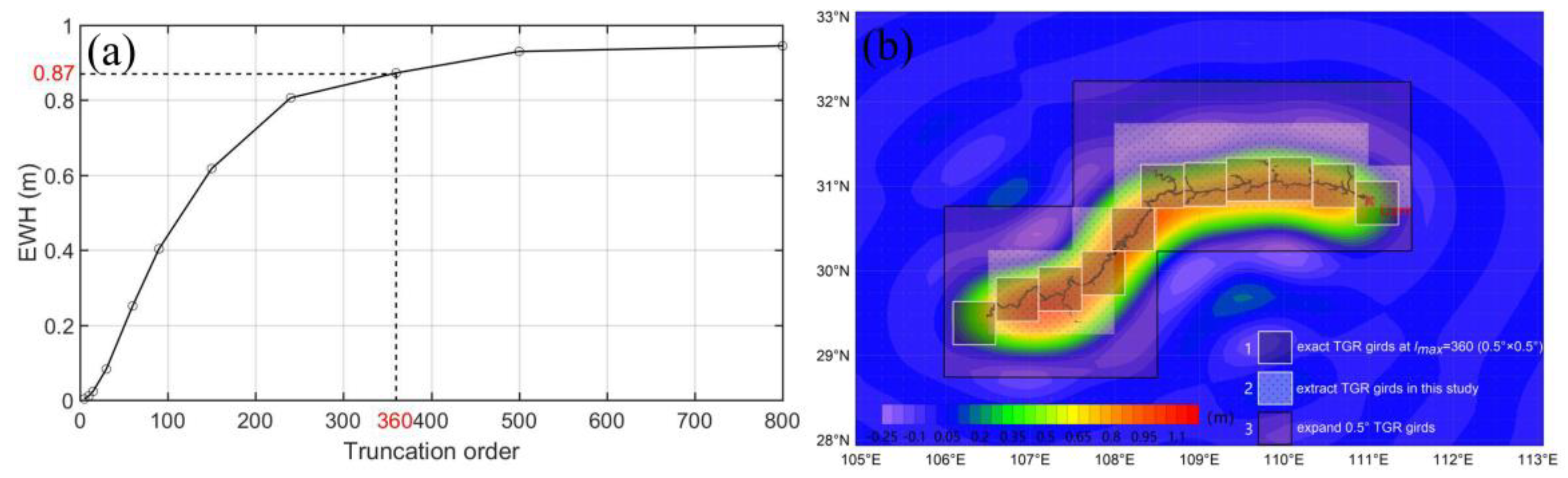
5.2. GRACE Spatial Resolution
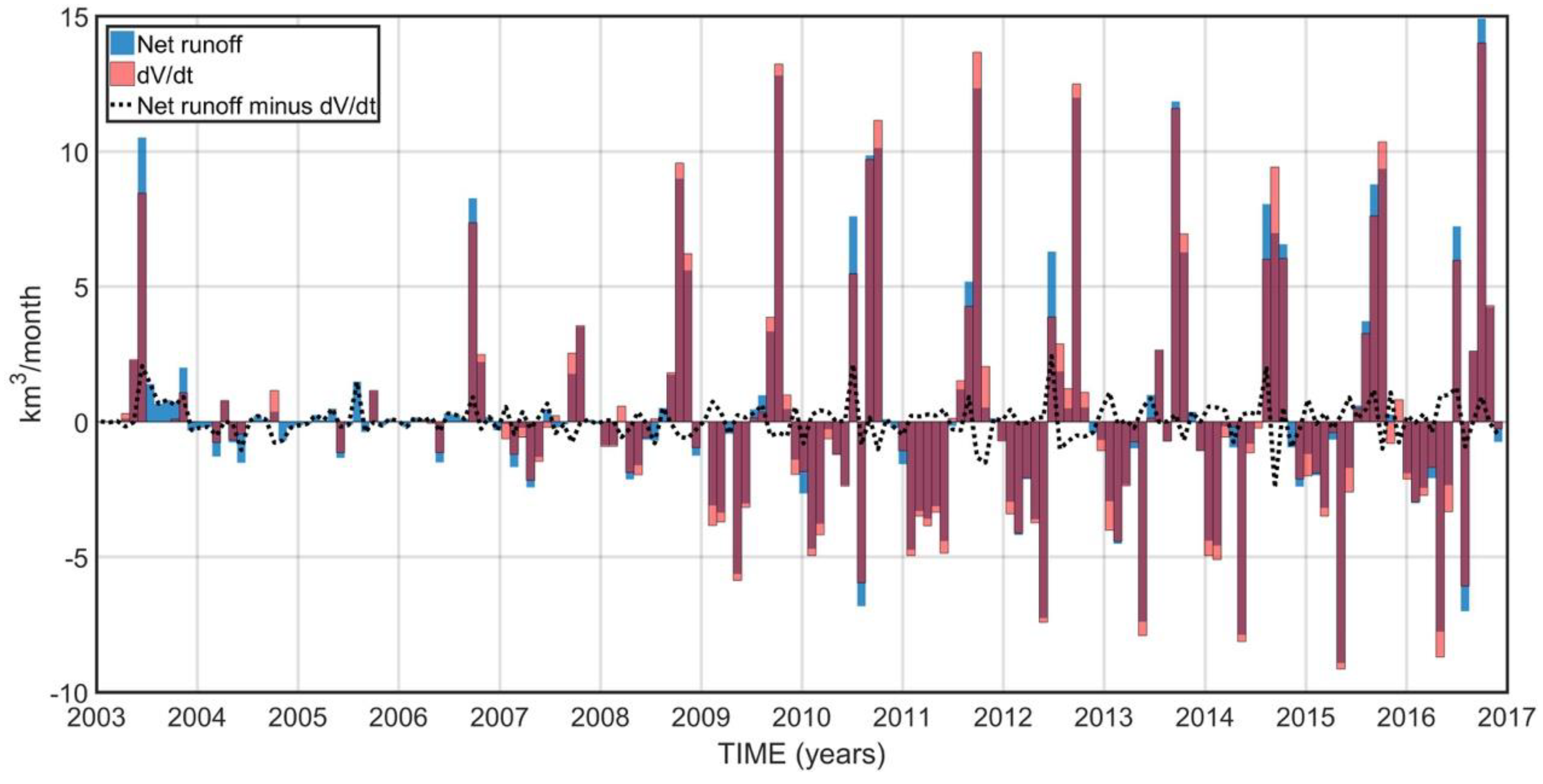
Traditionally, estimates of the mass change in a signal or certain region using GRACE were mainly based on the spatial average of the mass in the designated area with the sensitivity kernels. In the ideal case, the sensitivity in the region was one, and the sensitivity outside the region was zero. However, due to limitations of using the spherical harmonic coefficient order of the GRACE model (e.g., the highest order of GRACE gravity data used in this article is the 96th order, which provides a corresponding spatial resolution of about 2° × 2°), it is difficult for the region’s sensitivity kernel to reach a true one or zero. Therefore, the sensitivity kernel distribution obtained during the actual calculation for the TGR can not only provide insight into possible deviations in the estimated mass distribution using GRACE but can also help determine how to choose the size, shape, and location of mass-intensive areas.
As mentioned above, in order to obtain a higher resolution signal, the GRACE data was scaled based on the WGHM with a resolution of 0.5° × 0.5°. The restoration (downscaling) results significantly improved the signal amplitude and spatial differences in the study area, which indicated that the scale factor restoration (downscaling) method based on the LSM effectively improved the resolution of the original data. However, due to limitations in the resolution of the WGHM model, the signal could only be restored to a maximum 360th order, which is equivalent to a resolution of 0.5° × 0.5°, resulting in remaining signal ‘leakage’ (Figure 10a). Moreover, the WGHM is forced by a combination of a Global Precipitation Climatology Centre monthly precipitation datasets from 1901-present, which are calculated from rain gauge measurements and European Centre for Medium-Range Weather Forecasts analyses. Our comparison results show that the outputs of the WGHM agrees better with in-situ observations than GLDAS/Noah and CLM4.5 in the TGR area. But it also should be noted that the uncertainty in our estimated results from GRACE is largely affected by the amount of uncertainty from the WGHM model outputs.
In order to test the grid distribution suitable for signal extraction in the study area, a higher-resolution kernel distribution of equivalent water thickness sensitivity was constructed. A 1 m water level was set for each grid point, located in the range of 0.25° in the TGR, and the signal was truncated to the 360th order in the spherical harmonic domain to observe signal ‘leakage’. As shown in Figure 10b, grid area-1 was the most suitable area for TGR based on the current resolution. However, due to its irregularity, it could not cover signals that have obviously leaked to the external area. Therefore, when the internal signal of the region was extracted, the fit of the grid to the location of the actual reservoir area and the signal ‘leakage’ area was considered when possible. Grid area-3 showed a larger expansion range than the former two areas. The extraction of grid area-2 was closer to the true 1 m water height change, and the amplitude was much larger than grid area-3, which indicated that the area was too large and contained more external signals. This confirms the selection of grid area-2 for use in this study.

5.3. Runoff Effects

At the basin scale, GRACE data, precipitation data, and runoff data were used to estimate changes in ET in the TGR. The accuracy of regional runoff data will directly affect the final ET estimation results. The runoff data used in this study were the inflow and outflow of the TGD and Gezhouba dam. In order to analyze the impact of the difference between the inflow-outflow data and the actual regional runoff change, the net runoff of the TGD was compared with changes in the capacity of TGR based on water level changes (Figure 11).
It is noteworthy that the changes in the reservoir capacity of the TGR were mainly affected by the net runoff of the TGD, while the total effects of ET, precipitation, and surface-groundwater exchange were small. The maximum difference between the volume of the reservoir area and the dam’s runoff was reached in September 2014, of 2.4 km3/month, while the effect on the ET was about 4 cm/month, which was much less than the estimated ET at the corresponding time of 22 cm/month. In other periods, the difference between the two had an effect on ET of only about 1 cm/month. This result shows that the change in net runoff based on inflow and outflow data, which was not taken into account in the first half of the study area (the western end of the TGR), had little effect on the total runoff. The overall runoff in the TGR area was mainly controlled by the storage and release of the TGD during this time period.

5.4. Improving of Outputs of ET Products

The current ET products show obvious differences in certain regions and scales, and also have a large uncertainty [55,56]. The output value may be overestimated and underestimated at certain periods and regions. Our research results confirm that the ET is significantly observable by GRACE signals, with the improvement of GRACE signal accuracy and resolution, that could be good to consider assimilating the GRACE into the ET products to update their ET estimates. And Some scholars have already tried in this area and got good results [55].

6. Conclusions

The ET in the Three Gorges Reservoir area since the establishment of the Three Gorges Dam was estimated based on GRACE gravity data released by the CSR from 2002 to 2016 and surface hydrological observation data. The main conclusions were as follows:
(1)
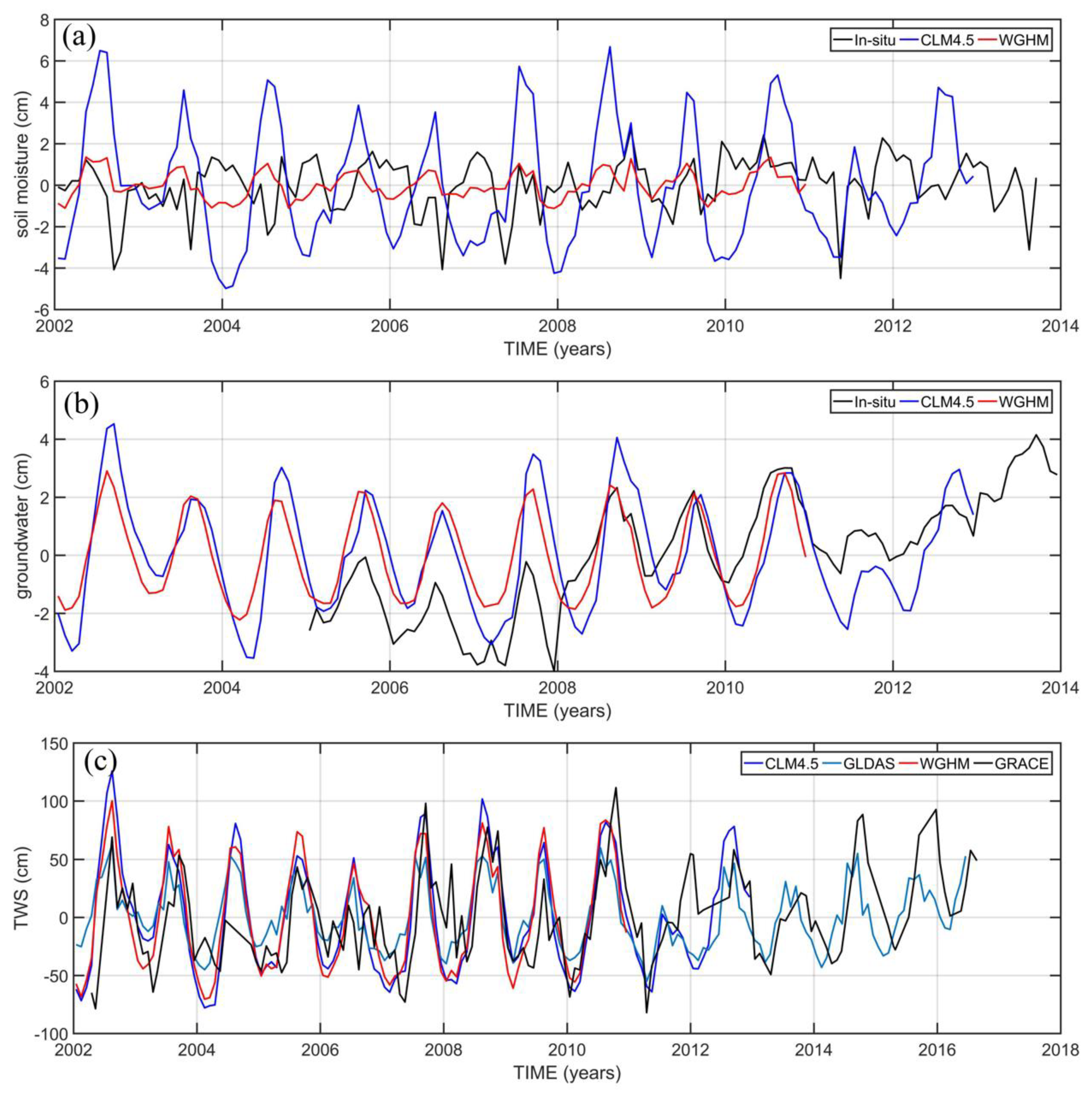
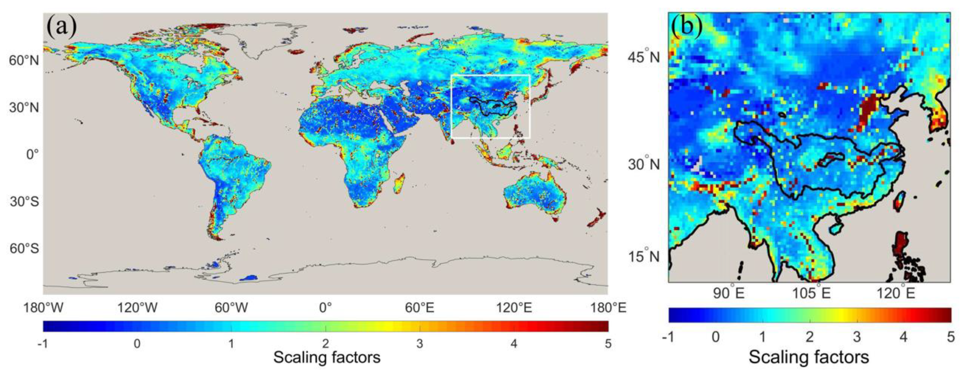
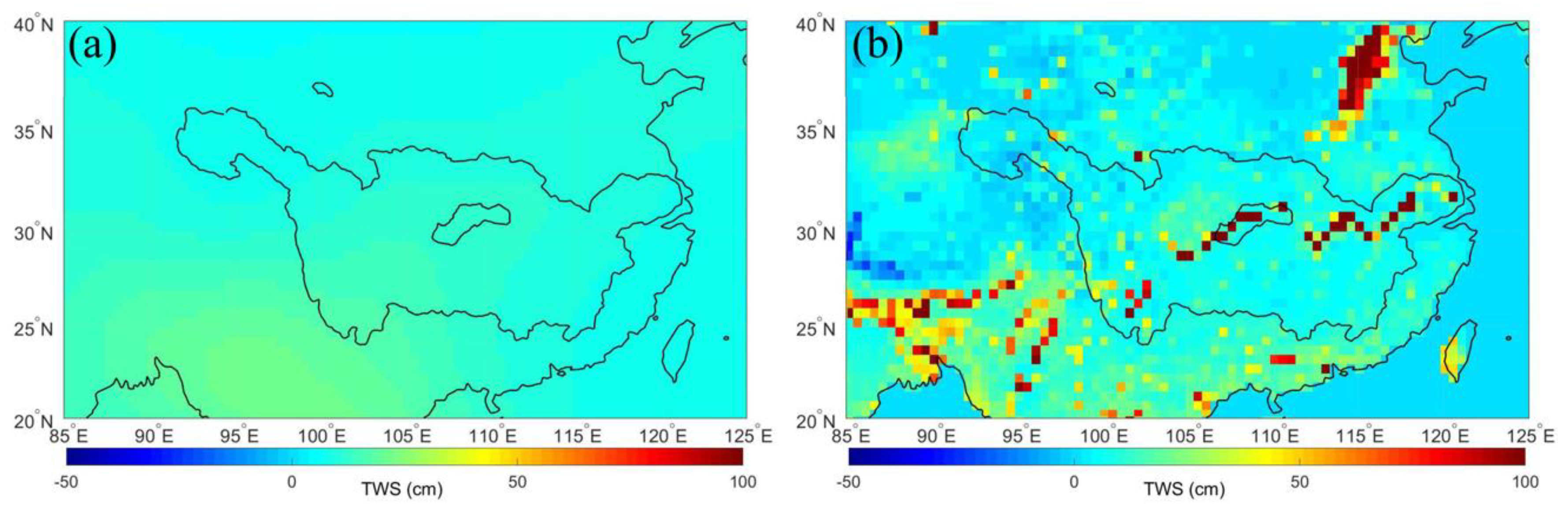
The WGHM and CLM4.5 Land System Models had higher credibility in the YRB and were able to describe the inter-annual change of terrestrial water reserves in the study area more accurately. However, GLDAS included soil and snow components that were not representative of the Yangtze River study area where the change in surface water content is dominant. The WGHM was selected based on the Nash efficiency coefficient to recover the signal ‘leakage’ caused by spherical harmonic truncation and Gaussian filtering. Our results indicated that the scaling factors derived by WGHM were good for enhancing the amplitude of the signal and improving the spatial resolution of the GRACE-driven TWS change.
(2)
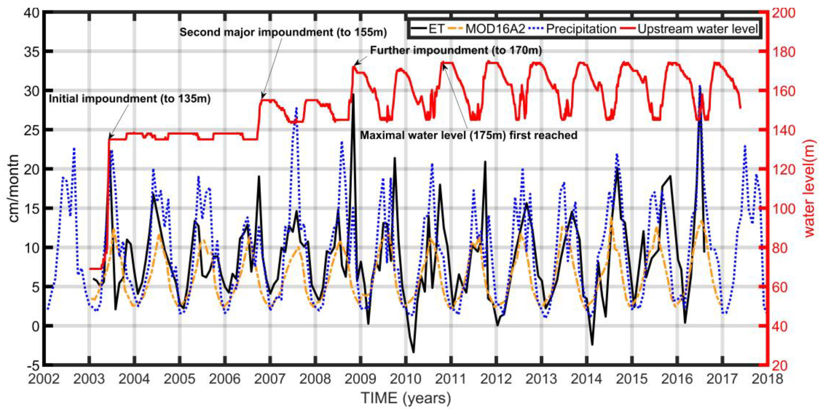
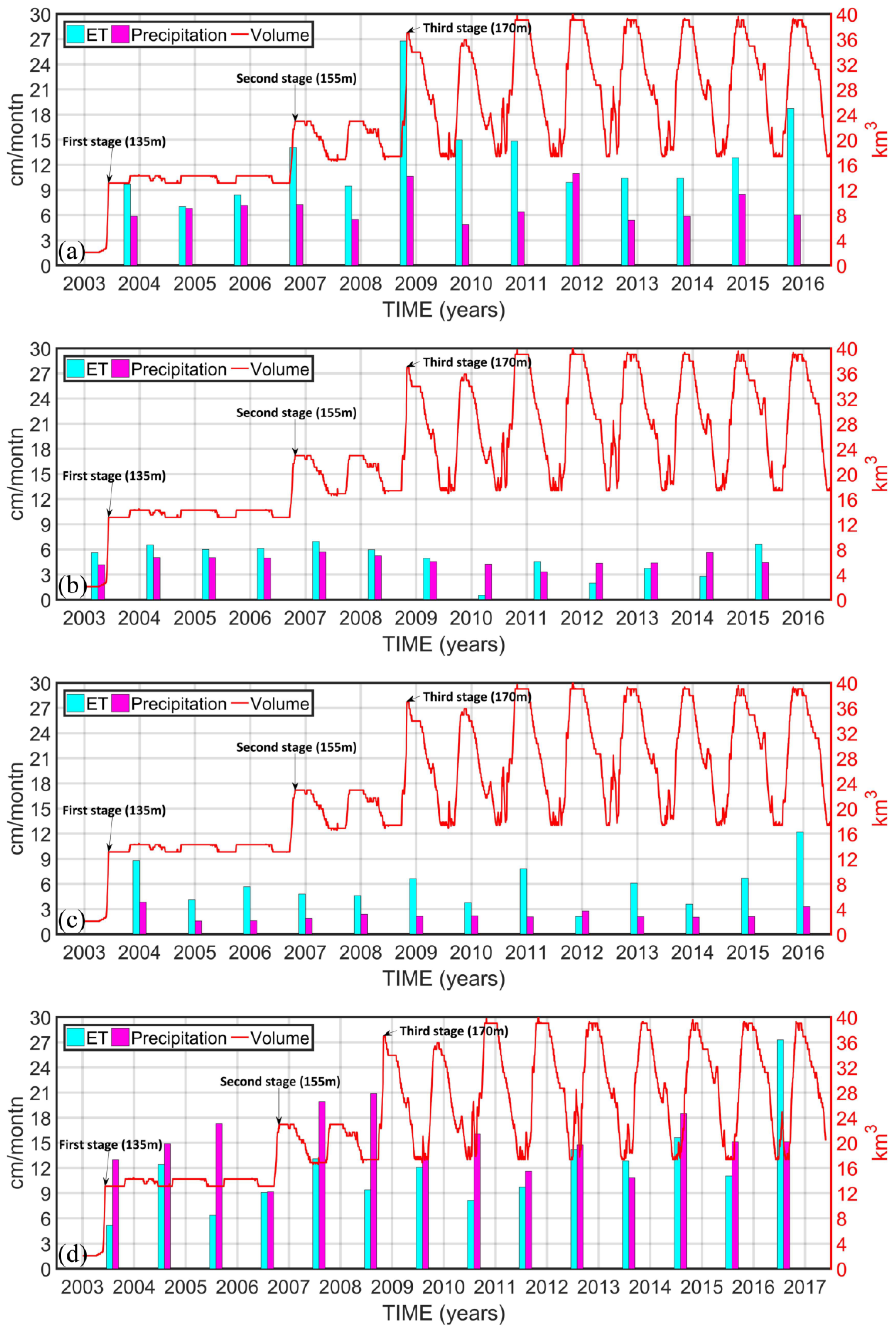
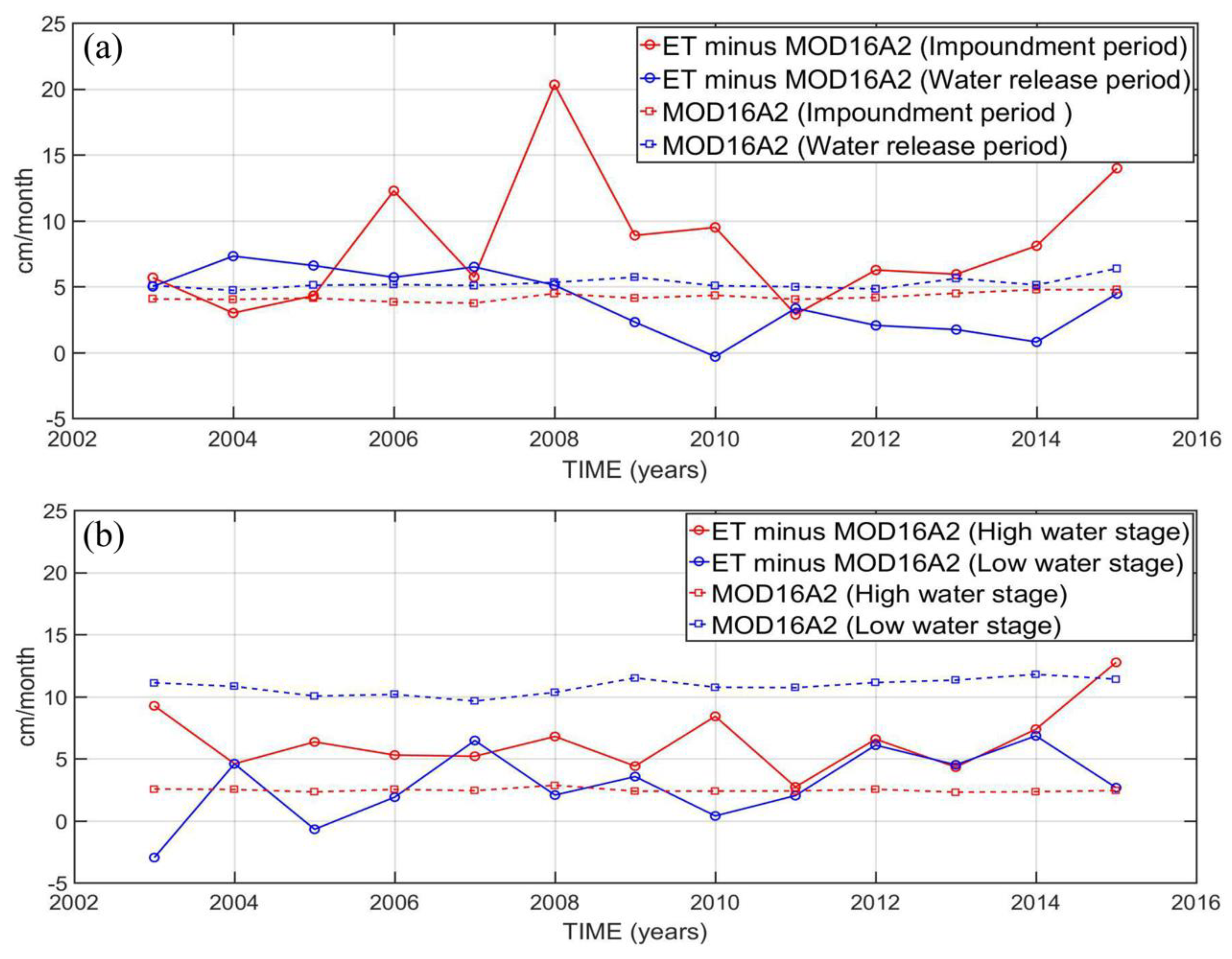
ET is affected by precipitation, water storage, and release events in the TGR. The seasonal changes in ET were mainly driven by rainfall. The fluctuations in the flooded area and storage capacity in the TGR were the main factors controlling the short-term changes in ET. Rising water levels during the storage stage led to an abnormal increase in regional ET. Water storage events in the TGR in 2003, 2006, and 2008 had the most obvious effects on ET. After that, the ET was abnormally reduced during the water release period (e.g., in spring and summer).
(3)
The MOD16A2 data product indicated that the ET from soil and vegetation was mainly driven by climate. The results showed no significant trends and abnormal fluctuations except for seasonal changes in the study area over the past ten years. The impact of the human-driven water storage and release events on the ET in the TGR area were mainly reflected in the mainstream and tributaries of the Yangtze River. The impacts of precipitation, ET, and surface-groundwater exchange maintained a dynamic balance compared with the impact of dam storage and release events at the basin scale.

Author Contributions

Conceptualization, L.W. and C.C.; Funding acquisition, L.W.; Methodology, Y.Z., L.W. and Z.P.; Investigation, Y.Z. and Z.F.; Supervision, L.W.; Validation, L.W. and C.C.; Writing—original draft, Y.Z.; Writing—review & editing, L.W., C.C. and Z.F. All authors have read and agreed to the published version of the manuscript.

Funding

This work is supported by the National Natural Science Foundation of China (41874090 and 41774091).

Acknowledgments

This work was supported by the National Natural Science Foundation of China (41874090 and 41774091). GRACE data in this study were provided by the CSR (ftp://podaac.jpl.nasa.gov/allData/grace/L2/CSR/RL06/). Remotely sensed evaporation data (MOD16A2-ET) was provided by NASA (https://ladsweb.modaps.eosdis.nasa.gov/archive/orders/). GLDAS data is provided by the NASA Goddard Geoscience Data and Information Services Center (http://disc.sci.gsfc.nasa.gov/). In addition, we also thank Prof. Andreas Güntner for providing the WGHM data published by the Goethe University Frankfurt, and the CLM4.5 data published by the National Center for Atmospheric Research provided by Prof. John Wahr. The measured groundwater and soil moisture data was sourced from the China Meteorological Data Sharing Service System (http://data.cma.cn/data/cdcindex.html). The water level and net runoff data of the Three Gorges Reservoir area are downloaded from the Yangtze River Three Gorges Corporation (https://www.ctg.com.cn/sxjt/sqqk/index.html).

Conflicts of Interest

The authors declare no conflict of interest.

References

  1. Syed, T.H.; Famiglietti, J.; Rodell, M.; Chen, J.; Wilson, C.R. Analysis of terrestrial water storage changes from GRACE and GLDAS. Water Resour. Res. 2008, 44, 02433. [Google Scholar] [CrossRef]
  2. Savenije, H.H.G.; Hoekstra, A.; Van Der Zaag, P. Evolving water science in the Anthropocene. Hydrol. Earth Syst. Sci. 2014, 18, 319–332. [Google Scholar] [CrossRef] [Green Version]
  3. Wang, J.; Sheng, Y.; Gleason, C.J.; Wada, Y. Downstream Yangtze River levels impacted by Three Gorges Dam. Environ. Res. Lett. 2013, 8, 044012. [Google Scholar] [CrossRef]
  4. Huang, Y.; Salama, M.S.; Krol, M.S.; Van Der Velde, R.; Hoekstra, A.; Zhou, Y.; Su, Z. Analysis of long-term terrestrial water storage variations in the Yangtze River basin. Hydrol. Earth Syst. Sci. 2013, 17, 1985–2000. [Google Scholar] [CrossRef] [Green Version]
  5. Zhan, S.; Song, C.; Wang, J.; Sheng, Y.; Quan, J. A Global Assessment of Terrestrial Evapotranspiration Increase Due to Surface Water Area Change. Earths Future 2019, 7, 266–282. [Google Scholar] [CrossRef] [PubMed] [Green Version]
  6. Mueller, B.; Hirschi, M.; Jimenez, C.; Ciais, P.; Dirmeyer, P.A.; Dolman, A.J.; Fisher, J.B.; Jung, M.; Ludwig, F.; Maignan, F.; et al. Benchmark products for land evapotran-spiration: LandFlux-EVAL multi-data set synthesis. Hydrol. Earth Syst. Sci. 2013, 17, 3707–3720. [Google Scholar] [CrossRef] [Green Version]
  7. Stan, F.-I.; Neculau, G.; Zaharia, L.; Ioana-Toroimac, G.; Mihalache, S. Study on the Evaporation and Evapotranspiration Measured on the Căldăruşani Lake (Romania). Procedia Environ. Sci. 2016, 32, 281–289. [Google Scholar] [CrossRef] [Green Version]
  8. Wang, X.; De Linage, C.; Famiglietti, J.; Zender, C.S. Gravity Recovery and Climate Experiment (GRACE) detection of water storage changes in the Three Gorges Reservoir of China and comparison with in situ measurements. Water Resour. Res. 2011, 47, 1091–1096. [Google Scholar] [CrossRef]
  9. Long, D.; Yang, Y.; Wada, Y.; Hong, Y.; Liang, W.; Yaning, C.; Yong, B.; Hou, A.; Wei, J.; Chen, L. Deriving scaling factors using a global hydrological model to restore GRACE total water storage changes for China’s Yangtze River Basin. Remote Sens. Environ. 2015, 168, 177–193. [Google Scholar] [CrossRef]
  10. Huang, Y.; Salama, M.S.; Krol, M.S.; Su, Z.; Hoekstra, A.; Zeng, Y.; Zhou, Y. Estimation of human-induced changes in terrestrial water storage through integration of GRACE satellite detection and hydrological modeling: A case study of the Y angtze R iver basin. Water Resour. Res. 2015, 51, 8494–8516. [Google Scholar] [CrossRef]
  11. McVicar, T.R.; Van Niel, T.; Li, L.; Hutchinson, M.F.; Mu, X.; Liu, Z. Spatially distributing monthly reference evapotranspiration and pan evaporation considering topographic influences. J. Hydrol. 2007, 338, 196–220. [Google Scholar] [CrossRef]
  12. Miralles, D.G.; Holmes, T.R.; De Jeu, R.A.M.; Gash, J.H.; Meesters, A.G.C.A.; Dolman, H. Global land-surface evaporation estimated from satellite-based observations. Hydrol. Earth Syst. Sci. 2011, 15, 453–469. [Google Scholar] [CrossRef] [Green Version]
  13. Rahimikhoob, A.; Asadi, M.; Mashal, M. A Comparison Between Conventional and M5 Model Tree Methods for Converting Pan Evaporation to Reference Evapotranspiration for Semi-Arid Region. Water Resour. Manag. 2013, 27, 4815–4826. [Google Scholar] [CrossRef]
  14. Yang, X.; Gourley, J.J.; Ren, L.; Zhang, Y.; Long, D. Multi-scale validation of GLEAM evapotranspiration products over China via ChinaFLUX ET measurements. Int. J. Remote Sens. 2017, 38, 5688–5709. [Google Scholar] [CrossRef]
  15. Mao, Y.; Wang, K. Comparison of evapotranspiration estimates based on the surface water balance, modified Penman-Monteith model, and reanalysis data sets for continental China. J. Geophys. Res. Atmos. 2017, 122, 3228–3244. [Google Scholar] [CrossRef]
  16. Zhang, K.; Kimball, J.S.; Nemani, R.; Running, S.W. A continuous satellite-derived global record of land surface evapotranspiration from 1983 to 2006. Water Resour. Res. 2010, 46. [Google Scholar] [CrossRef] [Green Version]
  17. Yang, S.L.; Zhang, J.; Xu, X.J. Influence of the Three Gorges Dam on downstream delivery of sediment and its environmental implications, Yangtze River. Geophys. Res. Lett. 2007, 34, 10401. [Google Scholar] [CrossRef]
  18. Dai, Z.; Liu, J. Impacts of large dams on downstream fluvial sedimentation: An example of the Three Gorges Dam (TGD) on the Changjiang (Yangtze River). J. Hydrol. 2013, 480, 10–18. [Google Scholar] [CrossRef]
  19. Li, S.; Xiong, L.; Dong, L.; Zhang, J. Effects of the Three Gorges Reservoir on the hydrological droughts at the downstream Yichang station during 2003–2011. Hydrol. Process. 2012, 27, 3981–3993. [Google Scholar] [CrossRef]
  20. Wang, L.; Kaban, M.K.; Thomas, M.; Chen, C.; Ma, X. The Challenge of Spatial Resolutions for GRACE-Based Estimates Volume Changes of Larger Man-Made Lake: The Case of China’s Three Gorges Reservoir in the Yangtze River. Remote Sens. 2019, 11, 99. [Google Scholar] [CrossRef] [Green Version]
  21. Zaitchik, B.F.; Rodell, M.; Reichle, R.H. Assimilation of GRACE Terrestrial Water Storage Data into a Land Surface Model: Results for the Mississippi River Basin. J. Hydrometeorol. 2008, 9, 535–548. [Google Scholar] [CrossRef]
  22. Shokri, A.; Walker, J.P.; Dijk, A.I.J.M.; Pauwels, V.R.N. On the Use of Adaptive Ensemble Kalman Filtering to Mitigate Error Misspecifications in GRACE Data Assimilation. Water Resour. Res. 2019, 55, 7622–7637. [Google Scholar] [CrossRef] [Green Version]
  23. Rodell, M.; Seneviratne, S.I.; Viterbo, P.; Höll, S.; Famiglietti, J.; Chen, J.; Wilson, C.R. Basin scale estimates of evapotranspiration using GRACE and other observations. Geophys. Res. Lett. 2004, 31, 183–213. [Google Scholar] [CrossRef] [Green Version]
  24. Long, D.; Longuevergne, L.; Scanlon, B.R. Uncertainty in evapotranspiration from land surface modeling, remote sensing, and GRACE satellites. Water Resour. Res. 2014, 50, 1131–1151. [Google Scholar] [CrossRef] [Green Version]
  25. Li, Q.; Luo, Z.; Zhong, B.; Zhou, H. An Improved Approach for Evapotranspiration Estimation Using Water Balance Equation: Case Study of Yangtze River Basin. Water 2018, 10, 812. [Google Scholar] [CrossRef] [Green Version]
  26. Klees, R.; Zapreeva, E.A.; Winsemius, H.H.C.; Savenije, H.H.G. The bias in GRACE estimates of continental water storage variations. Hydrol. Earth Syst. Sci. 2007, 11, 1227–1241. [Google Scholar] [CrossRef] [Green Version]
  27. Longuevergne, L.; Scanlon, B.R.; Wilson, C. GRACE Hydrological estimates for small basins: Evaluating processing approaches on the High Plains Aquifer, USA. Water Resour. Res. 2010, 46. [Google Scholar] [CrossRef]
  28. Landerer, F.W.; Swenson, S.C. Accuracy of scaled GRACE terrestrial water storage estimates. Water Resour. Res. 2012, 48, 04531. [Google Scholar] [CrossRef]
  29. Vishwakarma, B.D.; Horwath, M.; Devaraju, B.; Groh, A.; Sneeuw, N. A Data-Driven Approach for Repairing the Hydrological Catchment Signal Damage Due to Filtering of GRACE Products. Water Resour. Res. 2017, 53, 9824–9844. [Google Scholar] [CrossRef]
  30. Hu, X.G.; Chen, J.L.; Zhou, Y.H.; Huang, C.; Liao, X. Using GRACE spatial gravity measurements to monitor seasonal changes in water reserves in the Yangtze River Basin. Sci. China Ser. D Earth Sci. 2006, 36, 225–232. (In Chinese) [Google Scholar]
  31. Hervé, Y.; Lai, X.; Xijun, L.; Stéphane, A.; Jiren, L.; Sylviane, D.; Muriel, B.-N.; Xiaoling, C.; Shifeng, H.; Burnham, J.; et al. Nine years of water resources monitoring over the middle reaches of the Yangtze River, with ENVISAT, MODIS, Beijing-1 time series, Altimetric data and field measurements. Lakes Reserv. Res. Manag. 2011, 16, 231–247. [Google Scholar] [CrossRef]
  32. Ni, S.N.; Chen, J.L.; Li, J.; Liang, Q. Terrestrial water storage change in the Yangtze and Yellow river basins from GRACE time-variable gravity measurement. J. Geod. Geodyn. 2014, 34, 49–55, (In Chinese with English abstract). [Google Scholar]
  33. Zhang, Z.; Chao, B.F.; Chen, J.; Wilson, C. Terrestrial water storage anomalies of Yangtze River Basin droughts observed by GRACE and connections with ENSO. Glob. Planet. Chang. 2015, 126, 35–45. [Google Scholar] [CrossRef]
  34. Lv, M.; Ma, Z.; Yuan, X.; Lv, M.; Li, M.; Zheng, Z. Water budget closure based on GRACE measurements and reconstructed evapotranspiration using GLDAS and water use data for two large densely-populated mid-latitude basins. J. Hydrol. 2017, 547, 585–599. [Google Scholar] [CrossRef]
  35. Boy, J.P.; Chao, B.F. Time-variable gravity signal during the water impoundment of China’s Three-Gorges Reservoir. Geophys. Res. Lett. 2002, 29, 53–57. [Google Scholar]
  36. Wang, H.-S.; Wang, Z.-Y.; Yuan, X.-D.; Wu, P.; Rangelova, E.; Han-Sheng, W.; Zhi-Yong, W.; Xu-Dong, Y.; Patrick, W.; Elena, R. Water Storage Changes in Three Gorges Water Systems Area Inferred from Grace Time-Variable Gravity Data. Chin. J. Geophys. 2007, 50, 650–657. [Google Scholar] [CrossRef]
  37. Zhong, M.; Duan, J.; Xu, H.; Peng, P.; Yan, H.; Zhu, Y. Trend of China land water storage redistribution at medi- and large-spatial scales in recent five years by satellite gravity observations. Sci. Bull. 2008, 54, 816–821. [Google Scholar] [CrossRef] [Green Version]
  38. Cheng, M.; Ries, J.C.; Tapley, B.D. Variations of the Earth’s figure axis from satellite laser ranging and GRACE. J. Geophys. Res. Space Phys. 2011, 116. [Google Scholar] [CrossRef] [Green Version]
  39. Cheng, M.; Tapley, B.D.; Ries, J.C. Deceleration in the Earth’s oblateness. J. Geophys. Res. Sol. Earth 2013, 118, 740–747. [Google Scholar] [CrossRef]
  40. Swenson, S.; Chambers, D.P.; Wahr, J. Estimating geocenter variations from a combination of GRACE and ocean model output. J. Geophys. Res. Space Phys. 2008, 113. [Google Scholar] [CrossRef] [Green Version]
  41. AG, W.J.; Zhong, S. Computations of the viscoelastic response of a 3-D compressible Earth to surface loading: An application to Glacial Isostatic Adjustment in Antarctica and Canada. Geophys. J. Int. 2012, 192, 557–572. [Google Scholar] [CrossRef]
  42. Chen, J.; Wilson, C.R.; Tapley, B.D.; Blankenship, D.D.; Ivins, E.R. Patagonia Icefield melting observed by Gravity Recovery and Climate Experiment (GRACE). Geophys. Res. Lett. 2007, 34. [Google Scholar] [CrossRef]
  43. Wahr, J.; Molenaar, M.; Bryan, F. Time variability of the Earth’s gravity field: Hydrological and oceanic effects and their possible detection using GRACE. J. Geophys. Res. Sol. Earth 1998, 103, 30205–30229. [Google Scholar] [CrossRef]
  44. Swenson, S.; Wahr, J. Methods for inferring regional surface-mass anomalies from Gravity Recovery and Climate Experiment (GRACE) measurements of time-variable gravity. J. Geophys. Res. Space Phys. 2002, 107. [Google Scholar] [CrossRef] [Green Version]
  45. Velicogna, I.; Wahr, J. Measurements of Time-Variable Gravity Show Mass Loss in Antarctica. Science 2006, 311, 1754–1756. [Google Scholar] [CrossRef] [Green Version]
  46. Rodell, M.; Houser, P.; Jambor, U.; Gottschalck, J.; Mitchell, K.; Meng, C.-J.; Arsenault, K.R.; Cosgrove, B.; Radakovich, J.; Bosilovich, M.; et al. The Global Land Data Assimilation System. Bull. Am. Meteorol. Soc. 2004, 85, 381–394. [Google Scholar] [CrossRef] [Green Version]
  47. Döll, P.; Kaspar, F.; Lehner, B. A global hydrological model for deriving water availability indicators: Model tuning and validation. J. Hydrol. 2003, 270, 105–134. [Google Scholar] [CrossRef]
  48. Oleson, K.W.; Lawrence, D.M.; Bonan, G.B.; Feddema, J. Technical Description of Version 4.5 of the Community Land Model (CLM) NCAR Technical Note NCAR/TNG 503+STR; National Center for Atmospheric Research: Boulder, CO, USA, 2013; p. 420.
  49. Xie, P.; Arkin, P.A. Global Precipitation: A 17-Year Monthly Analysis Based on Gauge Observations, Satellite Estimates, and Numerical Model Outputs. Bull. Am. Meteorol. Soc. 1997, 78, 2539–2558. [Google Scholar] [CrossRef]
  50. Schneider, U.; Becker, A.; Finger, P.; Meyer-Christoffer, A.; Ziese, M.; Rudolf, B. GPCC’s new land surface precipitation climatology based on quality-controlled in situ data and its role in quantifying the global water cycle. Theor. App. Climatol. 2014, 115, 15–40. [Google Scholar] [CrossRef] [Green Version]
  51. Monteith, J.L.; Reifsnyder, W.E. Principles of Environmental Physics. Phys. Today 1974, 27, 51. [Google Scholar] [CrossRef]
  52. Nash, J.E.; Sutcliffe, J.V. River flow forecasting through conceptual models part I—A discussion of principles. J. Hydrol. 1970, 10, 282–290. [Google Scholar] [CrossRef]
  53. Wang, K.; Dickinson, R.E. A review of global terrestrial evapotranspiration: Observation, modeling, climatology, and climatic variability. Rev. Geophys. 2012, 50. [Google Scholar] [CrossRef]
  54. Pan, Y.; Zhang, C.; Gong, H.; Yeh, P.J.-F.; Shen, Y.-J.; Guo, Y.; Huang, Z.; Li, X. Detection of human-induced evapotranspiration using GRACE satellite observations in the Haihe River basin of China. Geophys. Res. Lett. 2017, 44, 190–199. [Google Scholar] [CrossRef]
  55. Ahmed, M.; Sultan, M.; Yan, E.; Wahr, J. Assessing and Improving Land Surface Model Outputs Over Africa Using GRACE, Field, and Remote Sensing Data. Surv. Geophys. 2016, 37, 529–556. [Google Scholar] [CrossRef]
  56. Zhong, Y.; Zhong, M.; Mao, Y.; Ji, B. Zhong Evaluation of Evapotranspiration for Exorheic Catchments of China during the GRACE Era: From a Water Balance Perspective. Remote Sens. 2020, 12, 511. [Google Scholar] [CrossRef] [Green Version]
Figure 1. Location of the study area. The black outer border area is the Yangtze River Basin (YRB) and the black inner border area is the study area (TGR). The red “X” is the location of the Three Gorges Dam (TGD).
Remotesensing 12 02143 g001
Figure 2. Time-series and trend of EWH in the TGR area from 2002 to 2016. The yellow dots and black line indicate GRACE monthly estimates, which average value has been removed. Blue dotted line represents long-term linear trend. Shaded areas are uncertainties in TWS from GRACE.
Remotesensing 12 02143 g002
Figure 3. Flow chart of the scale factor method, which was used to recover the GRACE signal ‘leakage’ based on results from the LSM models, the red frames mean this is a simultaneous step.
Remotesensing 12 02143 g003
Figure 4. Comparison of LSM components with measured data. Comparison of (a) CLM4.5, WGHM, and measured soil moisture content; (b) CLM4.5, WGHM, and measured groundwater content; (c) WGHM, GLDAS, CLM4.5, and GRACE total TWS. The GRACE results here are not decorrelated and show more high-frequency signals than the results in Figure 2.
Remotesensing 12 02143 g004
Figure 5. Global and Chinese regional scale factors based on WGHM. (a) Global map of regional scale factors; (b) the white box area in (a).
Remotesensing 12 02143 g005
Figure 6. EWH maps of the YRB before and after the signal ‘leakage’ restoration (using September 2010 as an example). The EWH (a) before restoration and (b) after restoration.
Remotesensing 12 02143 g006
Figure 7. Estimated ET in the TGR. The solid red line is the upstream water level of the TGD; the blue dashed line is the precipitation in the TGR area; the yellow dashed line is the MOD16A2 estimated ET; the solid black line is the estimated ET derived by GRACE.
Remotesensing 12 02143 g007
Figure 8. Changes in average ET and precipitation at different periods of each year. (a) Impoundment period (Oct. to Nov.); (b) water release period (Feb. to May.); (c) high-water stage (Dec. to Jan.); (d) low-water stage (Jul. to Aug.). The red curve is the storage capacity of the TGR, which is obtained by converting the water level: V ( H ) = 0.2985 × 1.0284 H [8].
Remotesensing 12 02143 g008
Figure 9. Variation of ET during different periods of each year in both main and tributary flows after MOD16A2 ET data was removed. ET during (a) the storage period (from Oct. to Nov.) and release period (from Feb. to May.), and; (b) the high-water level period (from Dec. to Jan.) and low water level period (from Jul. to Aug.).
Remotesensing 12 02143 g009
Figure 10. Effect of spherical harmonic truncation on the signal. (a) The effect of different order truncation on the signal amplitude of the study area, the red number represents the order and amplitude of the signal recovered in this study; (b) the signal spread of the TGR area caused by the 360th order truncation. Different grids represent different study areas.
Remotesensing 12 02143 g010
Figure 11. Variations and differences between the net runoff of the TGD and the reservoir capacity. dV/dt is the change of the reservoir capacity (V) of the TGD, where the relationship between the V and the upstream water level, H, is: V ( H ) = 0.2985 × 1.0284 H [8].
Remotesensing 12 02143 g011

