Abstract
Three-dimensional (3D) surface models, e.g., digital elevation models (DEMs), are important for planetary exploration missions and scientific research. Current DEMs of the Martian surface are mainly generated by laser altimetry or photogrammetry, which have respective limitations. Laser altimetry cannot produce high-resolution DEMs; photogrammetry requires stereo images, but high-resolution stereo images of Mars are rare. An alternative is the convolutional neural network (CNN) technique, which implicitly learns features by assigning corresponding inputs and outputs. In recent years, CNNs have exhibited promising performance in the 3D reconstruction of close-range scenes. In this paper, we present a CNN-based algorithm that is capable of generating DEMs from single images; the DEMs have the same resolutions as the input images. An existing low-resolution DEM is used to provide global information. Synthetic and real data, including context camera (CTX) images and DEMs from stereo High-Resolution Imaging Science Experiment (HiRISE) images, are used as training data. The performance of the proposed method is evaluated using single CTX images of representative landforms on Mars, and the generated DEMs are compared with those obtained from stereo HiRISE images. The experimental results show promising performance of the proposed method. The topographic details are well reconstructed, and the geometric accuracies achieve root-mean-square error (RMSE) values ranging from 2.1 m to 12.2 m (approximately 0.5 to 2 pixels in the image space). The experimental results show that the proposed CNN-based method has great potential for 3D surface reconstruction in planetary applications.
1. Introduction
Three-dimensional (3D) reconstruction is used to reconstruct 3D models of objects; these include digital elevation models (DEMs) of terrain surfaces, which are critical for planetary science and engineering research such as landing-site selection [1,2,3], geomorphological research [4], morphometric analyses [5,6], and geological studies [7]. Existing DEMs of the Martian surface include the Mars Orbiter Laser Altimeter (MOLA) DEM [8], which is generated by laser altimetry, and photogrammetry-based DEMs based on images from the High-Resolution Stereo Camera (HRSC) DEMs [9], context camera (CTX) DEMs [10], and the High-Resolution Imaging Science Experiment (HiRISE) DEMs [11]. The DEMs generated by laser altimetry usually have low resolution [8,12]. Thus, photometric-based DEMs are widely used [13]. Photogrammetry requires stereo or multiple images with appropriate geometry, and the resulting DEMs typically have resolutions 3–10 times lower than that of the original images, depending on the textural conditions of these images [14]. For planetary surfaces, such as those on Mars, high-resolution stereo images are rare [15].
Shape-from-shading (SfS), or photoclinometry, has been developed and applied in planetary topographical mapping for decades and has shown promising performance [16,17,18,19]. The SfS technique reconstructs a 3D surface from a single image by evaluating the photometric contents of each pixel and then generating a DEM with the same resolution as the input image. However, the thin Martian atmosphere attenuates the measured radiance, which leads to ambiguities in the SfS analysis, and the additional preferred atmospheric parameters that are used to reduce the effects of such ambiguities are difficult to obtain on Mars. Thus, applying SfS to images of Mars is challenging.
In recent years, convolutional neural networks (CNNs) have achieved great success in multiple image tasks. Unlike traditional methods, CNN-based methods can study and recognize features implicitly from a large dataset that contains thousands of samples, from which useful information is automatically extracted and memorized [20]. CNNs have generated promising 3D reconstruction results from close-range images, street maps [21,22,23,24,25], and face images [26,27,28,29,30]. The principle of CNN training, whereby the relationships between inputs and outputs are studied directly, ensures that ambiguities (such as noise and uncertainties) are implicitly learned and eliminated. These capabilities mean that CNN is particularly suited to the 3D reconstruction of the Martian surface, which is influenced by atmospheric ambiguities. To this end, Chen et al. [31] proposed a CNN-based algorithm for 3D reconstruction of the Martian surface that showed preliminary but favorable results.
This paper proposes a CNN-based framework for the 3D reconstruction of the Martian surface, with the network comprising two subnetworks. The auto-denoising network predicts reconstructed images and a correction term for the images, and then it calculates Lambertian images devoid of albedo differences and noise. The 3D reconstruction network generates high-quality DEMs based on the results from the auto-denoising network. Unlike previous work [31], our method considers elements that cause ambiguities in the 3D reconstruction process, such as atmospheric effects, albedo variations, and image noise. The performance of the proposed network is evaluated using real Martian remote-sensing imagery and DEMs. The remainder of this paper is organized as follows. Section 2 reviews the related literature. Section 3 provides details of the proposed method. In Section 4, we report the results of experiments conducted using CTX images of typical landforms on the Martian surface, and the performance of the network is evaluated. A discussion and conclusions are presented in Section 5 and Section 6, respectively.
2. Related Work
Here, we review related work on 3D surface reconstruction from single images. Traditional 3D reconstruction techniques (e.g., photogrammetry and laser altimetry) are ignored, as they are outside the scope of this paper.
3D surface reconstruction methods based on single images, such as SfS and shape-and-albedo-from-shading (SAfS), have been successfully applied in lunar topographical mapping [16,17,18,19] and landing-site assessments of Mars [32,33,34]. These techniques analyze the intensity of image pixels and how the planetary surface reflects incoming irradiance, such as sunlight. In general, the SfS technique contains solutions to partial differential equations (PDEs) and optimization. In PDE solutions, the SfS problem is addressed in several partial differential equations, and the research goal is to solve these equations. “Viscosity solutions” were proposed by Rouy and Tourin [35] to solve first-order PDEs. The Markov chain approximation algorithm was later proposed by Oliensis and Dupuis [36]. However, viscosity solutions can cause ambiguities known as “concave/convex ambiguities”, as described by Horn [37], due to the method’s lack of uniqueness. Several attempts have been made to overcome this problem by applying a “maximal solution” [38,39].
In recent years, optimization methods have become very popular. Early optimization methods estimated the gradient of a surface by assuming a reflectance model that is connected to the relationships between the gradients and intensity values of the pixels [40,41]. Barron and Malik [42,43] proposed the SAfS method, where albedo is the optimized target. In their work, both albedo and shape are incorporated in loss functions and optimized together until they converge. Tenthoff et al. [44] applied SfS to generate DEMs of Mercury, and the algorithm enabled the process to work properly under multiple image mosaics and substantial albedo variations.
The atmosphere of Mars makes the photometric process more complex than it is for airless bodies. The incoming sunlight is attenuated and scattered by aerosols in the atmosphere, causing both direct and indirect illumination of the surface. The reflected sunlight from the surface is also subject to similar effects before reaching the sensor. Early attempts to apply SfS/SAfS to Mars 3D image reconstruction tended to ignore or approximate the atmospheric effects or incorporated additional information, such as data from spectroscopic observations or multiple simultaneously acquired images (e.g., HRSC). These factors limit the use and performance of this technology.
CNN-based 3D reconstruction methods using single images are well developed for the generation of depth maps of close-range images and street maps. Eigen et al. [22], who were the first to use a CNN to predict depth maps, generated a coarse-depth prediction result that was integrated with another block to afford a refined prediction. The predicted depth maps had one-quarter the resolution of the input images. Laina et al. [21] proposed a fully convolutional network in which the fully connected layer is replaced to achieve real-time prediction. In addition, to accelerate the processing speed, a faster up-convolution block was designed that integrates several convolution results for up-sampling [21]. Cao et al. [23] converted the regression problem to a classification problem to simplify the task. Some researchers have added auxiliary information to the network to achieve better performance. Ma and Karaman [25] added sparse depth samples from point cloud data to the network, which improved the accuracy by more than 50%. Aside from depth maps, the output of CNNs has variable formats, such as mesh polygon and point clouds, to describe 3D information when using a single image as the input [45]. Fan et al. [46] and Xia et al. [47] proposed methods that output a group of point coordinates to describe 3D information. Pontes et al. [48] proposed a network that generates 3D mesh models and refining parameters to optimize the models simultaneously.
However, CNNs have been less explored for planetary 3D reconstruction. Thus, we propose a CNN-based framework to achieve high-resolution 3D reconstruction of the Martian surface using single images.
3. A CNN-Based Method for 3D Reconstruction of the Martian Surface from Single Images
3.1. Overview of the Proposed Approach
Figure 1 and Figure 2 show overviews of the proposed CNN training and 3D reconstruction methods. Both synthetic and real datasets were used to train the network. The synthetic data comprised simulated DEMs and images, and the real datasets comprised CTX imagery and HiRISE DEMs obtained from the Mars Orbital Data Explorer website. The data format of the CTX images was the projected image from the converted raw image into reflectance (Map-projected Radiometric Data Record, MRDR) with 8-bit pixel depth, and the image depth of HiRISE DEMs was 32 bits. These data were used as the real-world training dataset, the validation dataset, and the test dataset. CTX images and DEMs were normalized to zero mean and unit standard deviation in the pre-processing step by computing the standard score of each pixel, with the purpose to help the network to recognize patterns better and to reduce the effects of atmospheric haze and solar incidence angle. The network was first trained using synthetic training data to prevent the underfitting phenomenon. After several epochs, these training data were replaced by the real-world training data, and the network was trained for several more epochs. If the network performance met expectations, the test data were introduced to evaluate the network performance and ensure that the well-trained network was ready for use in 3D reconstruction tasks. In the 3D reconstruction process, CTX images were fed into the well-trained network. Because the normalization step removes absolute scales, the CNN-predicted DEMs were then scale-recovered based on the correlation between the standard deviation of image intensity and the gradients along the illumination direction. The scale recovery was further refined using existing low-resolution DEMs (e.g., the MOLA DEM) covering the same area.
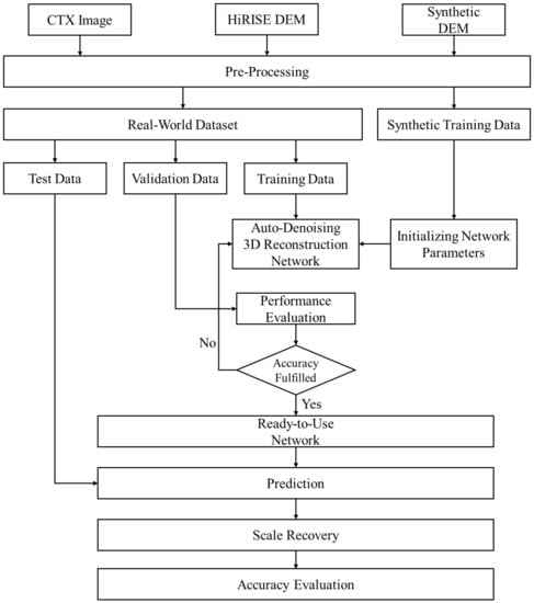
Figure 1.
Flowchart of the convolutional neural network (CNN) training process.
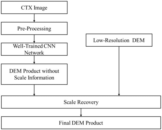
Figure 2.
Flowchart of the 3D reconstruction process.
3.2. Datasets
In this study, the synthetic dataset, CTX images, and the HiRISE DEM were utilized for training and evaluating the performance of our proposed algorithm. Examples of images are shown in Figure 3. Because the size and number of available HiRISE DEMs are limited, they were not adequate for training the CNN. Moreover, the standard data augmentation methods such as flip and rotation violate the relation between the pixel value and topographic gradients along the illumination direction. Therefore, a synthetic dataset was constructed to ensure satisfactory performance. All data consisted of orthoimages, corrected images, Lambertian images (i.e., the Lambertian reflectance of the surface), and DEMs corresponding to the orthoimages.
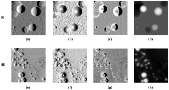
Figure 3.
Examples of two types of datasets: (i) synthetic images; (ii) real images. (a) Simulated image; (b) Lambertian image; (c) corrected image; (d) synthetic DEM; (e) CTX image; (f): Lambertian image from the HiRISE DEM; (g) corrected image; (h) HiRISE DEM.
3.2.1. Synthetic Dataset
A synthetic dataset offers well-initialized parameters for later fine-tuning using real datasets. The synthetic DEM consisted of the three typical terrain types on Mars: craters, cones, and random slopes. To generate a synthetic DEM with a pre-defined size of φ × φ nodes, the following equation is used:
where h is the generated DEM; S is a spherical function used to represent craters; E is an ellipsoid function for representing cones; G is Gaussian noise; and k and l are the pixel coordinates of the DEM. are the center coordinates and radius of sphere i, and are the center coordinates and the two major axes of ellipsoid j. α and β are random positive numbers indicating the number of corresponding landforms to be generated, and coordinates were randomly selected within the range of 0 to 224.
After the DEMs were generated, the Lommel–Seeliger reflectance model was used to generate synthetic images for use as simulated input images. An example of a simulated input image is presented in Figure 3a. The isotropic Lommel–Seeliger reflectance model [49] is expressed as shown in the following function:
where A is the albedo, which is regarded as a constant. μ0 and μ are the cosines of the incidence and emission angles. We assume that the azimuth of illumination direction I is 270°, the elevation angle is 45°, and the camera direction C is perpendicular to the surface level. η(k, l) indicates the surface normal. μ0 and μ are defined by the following respective equations:
and the surface normal is defined as follows:
The surface normal is expressed as a vector.
To generate images that remove noise and albedo effects, like the example shown in Figure 3b, the Lambertian reflectance law was also considered, which is expressed as follows:
Finally, a corrected image was introduced to convert the two reflectance laws, as shown in Figure 3c. The relationship between the synthetic and Lambertian images can be expressed as
From Equation (2), the corrected image is defined as
To initialize the network parameters of the synthetic dataset, we generated 70,000 patches of 224 × 224 pixels in size. The initialized CNN was then further fine-tuned using a real-world dataset, and the actual photometric characteristics of the Martian surface were learned during the training.
3.2.2. Real-World Dataset
We collected approximately 10,000 patches of CTX images paired with HiRISE DEMs from the Mars Orbital Data Explorer (https://ode.rsl.wustl.edu/mars/, accessed on 1 December 2020) to use as training samples and labels in our real-world dataset. The first pre-processing step was to normalize the images and DEMs to zero mean and unit standard deviation, which reduces atmospheric effects and enhances CNN effectiveness. The second step involved unifying their spatial resolutions to 6 m/pixel and then rotating them to an illumination direction with an azimuth of 270°. Synchronizing illumination directions minimizes unnecessary uncertainties and consequently increases the network’s performance. We assumed that the CTX images followed Lommel–Seeliger reflectance. As there may be atmospheric attenuation, shadows, and camera noise in the CTX images, the formula of the corrected image was modified to
where is the term indicating possible atmospheric effects and noise. An example of a corrected image from a real CTX image is shown in Figure 3g. All images were truncated to patches 224 × 224 pixels in size.
3.3. Network Architecture
As shown in Figure 4 the network consists of two subnetworks. The auto-denoising network removes possible albedo variations, atmospheric effects, and noise from input images by converting them to Lambertian images. This auto-denoising network has two deconvolution sections: the first reconstructs the input images, and the second predicts the corrections between the input images and the desired Lambertian images based on Equation (7). The 3D reconstruction network reconstructs 3D surfaces from the Lambertian images. A two-stage network can reduce possible contamination by noise and increase the stability of reconstruction. It also allows for performance evaluation of individual subnetworks. The backbone network for both subnetworks is the Inception-Resnet-V2 [50], which was chosen because it is well balanced in factors including computational constraints, data availability, and network performance. The deconvolution block consists of five up-sampling groups. Concatenation paths were added between the convolution and deconvolution blocks in the same subnetwork in order to integrate low-level and high-level features [51] and achieve better performance. As the traditional deconvolution operation generates extensive noise, it was replaced by combining a bilinear interpolation layer with a normal convolution layer [52].
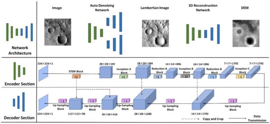
Figure 4.
Network architecture.
The activation function of the backbone network is the rectified linear unit (ReLU) function [53], which is defined by the following formula:
where represents the tensors among layers.
To constrain the range of the corrected image to (0,1), a sigmoid function was applied in the last layer of the correction deconvolution section, as shown below:
The activation function in the 3D reconstruction deconvolution section is the simplified S-shaped ReLU (SReLU) function [54], which is able to account for the possible height range of planetary surfaces while maintaining the advantages of ReLU. The SReLU function is expressed by the following formula:
3.4. Loss Function
The standard loss function for regression tasks is the loss, which minimizes the squared differences between the predicted and the labeled (ground truth) . However, in our experiment, the loss was found to generate over-smoothed predictions. Therefore, the Huber loss was used as the loss function in this research, and it is defined as follows:
For the auto-denoising network, the loss of the corrected images and the loss of the Lambertian images were calculated individually. The overall loss function of the auto-denoising network is defined as follows:
where is the regularization parameter, which equals 1 × 10⁻⁵. is the normalization item that was used to diminish overfitting, which is defined as follows:
where represents all of the parameters of the network.
In the 3D reconstruction network, the Huber loss of the elevations was calculated, and a first-order matching term was introduced to learn similar local structures based on the ground truth [24]. The first-order matching term is defined as follows:
The overall loss function of the 3D reconstruction network is given as follows:
with = 0.5, which was determined empirically based on experiments.
3.5. Training Strategy and Implementation
In the proposed network, the two subnetworks were trained separately. First, the loss of the auto-denoising network was calculated, and its parameters were updated. Then, the Lambertian surface images generated by the first auto-denoising network were fed into the 3D reconstruction network, and the loss of the second block was calculated separately. The two subnetworks were separately trained because if the entire set of network parameters are updated together, the 3D reconstruction loss of the 3D reconstruction network decreased the quality of the Lambertian surface images generated by the auto-denoising network. Moreover, the learning rates of these two tasks differed and were set individually. As we had two datasets, the synthetic dataset was utilized first to train the network. We found that when using the synthetic data with an increasing number of training epochs, the network tended to depict more small details on the input images, some of which were artificially generated noise. This tendency was difficult to inhibit by utilizing the real-world dataset. Thus, our strategy was to first train the network using the synthetic dataset for approximately five epochs and then use the real-world dataset for the remaining training epochs. After 10 epochs, the network was ready for prediction and performance assessments. The metric used to determine the performance of the network was the overall loss, shown in Equation (17), of the test data.
The network was built on the TensorFlow 1.14.0 platform [55] and implemented on a single RTX 2080Ti graphic card. The Adam optimizer was used for both network blocks with different learning rates of 3 × 10⁻⁴ and 5 × 10⁻⁵, with default values used for the other hyperparameters [56]. The batch size was set to four.
3.6. Scale Recovery
The CNN prediction results had a normalized scale and were rotated from the normalization of the illumination azimuth. Post-processing was performed to recover the correct direction and elevation of the predicted 3D models. The predicted patches were first mosaicked and rotated back to their original direction. Then, the elevation scale was estimated and recovered, as described in the following.
Scale recovery is a critical problem, as the elevations of small surface targets cannot be determined by auxiliary low-resolution DEMs. Predicted DEMs have only relative elevations, and the correct scale corresponding to real-world elevations must be recovered. As shown in Figure 5, we found that the standard deviation of the CTX images and the standard deviation of gradients along the illumination direction of the HiRISE DEMs, had a positive correlation. This is because image values inherently represent the local topography (i.e., topographic shading), which is in principle the same as SfS, as SfS reconstructs surface slopes and heights using image intensities as clues. By statistical analysis, the corresponding can be estimated as follows:
where and are linear regression parameters, as depicted in Figure 5. The scale between the ground-truth elevations and the predicted DEMs can then be calculated as follows:
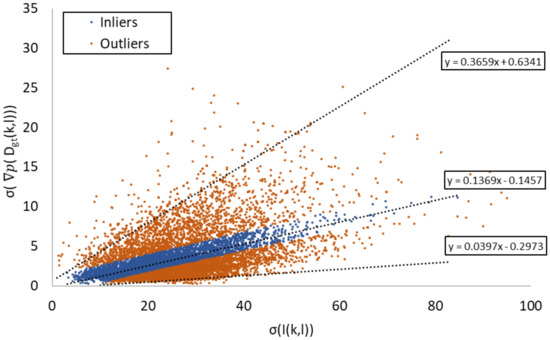
Figure 5.
Relationship of and . The inliers were selected by RANSAC [57], and parameters a and b calculated using the inliers were used as initial values for prediction.
Then, the elevation amplitude can be recovered as follows:
Figure 5 shows the global relationship of all of the CTX images and HiRISE DEMs used in the training process. The inliers (blue dots) represent the average relationship of the entire dataset, and they indicate strong correlations between the standard deviations of the image intensities and gradients in 3D space along the illumination direction. The correlation function (as depicted by parameters a and b) of the inliers can be used as the initialized value for scale recovery. In actual practice, the values of and can be further refined based on the available low-resolution DEM corresponding to the input image. The dispersion of dots in Figure 5 is affected by factors such as variations in photometric characteristics and the consistency of illumination and atmospheric conditions of the selected images. Therefore, images that have similar photometric behavior and incidence angles, as well as fewer variations in albedo and atmospheric haze, would reduce such dispersion and generate more accurate regression parameters.
Predictions from the network contain only high-frequency elevation information. To obtain global trends and determine absolute elevations, constraints from available low-resolution DEMs are needed to provide low-frequency information. To integrate both high-frequency information from the CNN predictions and low-frequency information from the existing low-resolution DEM, high-frequency information was first extracted from the predictions as follows:
where is the prediction generated by the CNN, and is the Gaussian filter.
The final output DEM integrates both frequencies as follows:
where represents the low-resolution DEM.
4. Experimental Evaluation
The performance of the proposed method was evaluated using single CTX images and their corresponding HiRISE DEMs. The evaluation was divided into two parts. The performance of the proposed auto-denoising network was evaluated first, and then the performance of the entire network was evaluated further. The structural similarity (SSIM) index was introduced to evaluate the similarity between images and inverted Lambertian images from DEMs [58]. Given two images x and y, the equation of SSIM is defined as
where and are the respective mean values of images x and y, is the covariance of images x and y, and and are constants. The range of the SSIM index is from 0 to 1. Higher values mean the images are more similar to each other. SSIM offers an indication of structural similarity between images and is more robust to random noise. Because the Lambertian images inverted from the HiRISE DEMs inherit a certain amount of noise, SSIM is a more appropriate indicator than the conventional correlation coefficient. Typical landforms on the Martian surface were chosen, such as craters, gullies/canyons, sand dunes, and cones. HiRISE DEMs were used as the ground truth for comparison, and these were down-sampled to realize the same 6 m/pixel resolution as the CTX images. Low-resolution DEMs with a spatial resolution of 463 m/pixel (similar to the spatial resolution of the MOLA DEM) were also interpolated from the HiRISE DEMs.
4.1. Evaluations of the Auto-Denoising Network
Three image patches from CTX mosaics were chosen to evaluate the performance of the auto-denoising network. In Figure 6, three patches containing albedo variations or noise are presented. These problematic features were successfully removed or minimized by the denoising. Table 1 also shows that the optimized images and Lambertian images generated by the DEMs had better SSIM index values, which validates the performance of the proposed network. However, for some regions of severe contamination, the network could not adjust differences perfectly. Distinguishing extreme values caused by different elements is difficult for the current network. In addition, as in most CNN implementations, the network first normalized the images before training. The normalization involves subtracting the mean value from each pixel and then dividing by the standard deviation (i.e., the standard score of each pixel of a 224 × 224 image patch). We found that the normalization step can partially reduce the effects of atmospheric attenuation and haze offset, which ensures the performance of the first subnetwork.
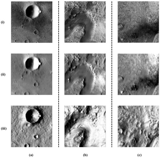
Figure 6.
Examples of CTX images and optimized images from the auto-denoising network: (i) CTX images; (ii) optimized images; (iii) simulated Lambertian images. (a) F21_043841_1654_XN_14S184W, (b) J03_045994_1986_XN_18N282W, (c) J03_045994_1986_XN_18N282W.

Table 1.
Comparison of structural similarity (SSIM) values.
4.2. Evaluations of Different Landforms
The results of evaluations of four typical landforms, i.e., sand dunes, gullies, cones, and craters, are presented and discussed in this section. Table 2 presents the details of the chosen datasets. Selected profiles and 3D surfaces obtained by prediction and ground truth are provided for evaluating the performance of the proposed method. Table 3 shows the calculated root-mean-square error (RMSE) values for the differences between the elevations predicted by the CTX images before and after merging the low-resolution DEMs and the ground-truth elevations obtained by the HiRISE DEMs. The root mean square (RMS) value of the elevations is also given.
Table 2.
Information on the test datasets.
Table 3.
Experiment results for four types of landforms.
As shown in Figure 7, relative to the HiRISE DEM, sand dunes were well reconstructed from the CTX image, except for a missing part of the middle image. However, the missing part was not present in the CTX image either. This may be because the missing dune is too small to be visible under the specified illumination conditions, or because it changed slightly due to the different acquisition times of the CTX and HiRISE images. In the bottom region, the ground-truth elevation was also lower than the predicted elevation. This is because the low-resolution DEM interpolated from the HiRISE DEM could not provide sufficient elevation details to enable scale recovery. The sand dune dataset had an RMSE value of 7.4 m.
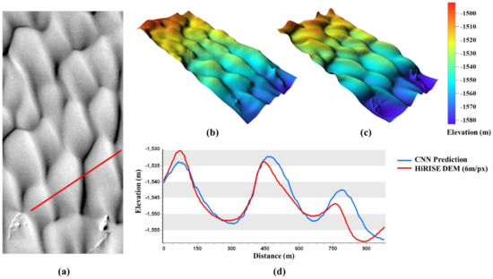
Figure 7.
Sand dune 3D reconstruction results: (a) CTX image; (b) 3D surface generated by the proposed method; (c) 3D surface generated by a HiRISE DEM; (d) Comparison of the selected profiles.
As shown in Figure 8, gullies were also well reconstructed. The reconstructed surface was smoother than that of the HiRISE DEM. In Figure 8d, which shows a comparison of the profile of the reconstructed surface with that of the ground truth, the depth of the gully is appropriate, but the ridges along the gully are higher than those in the HiRISE DEM. The occurred because the pixels of the ridges were much brighter than those in other regions of the image, which led to a prediction bias. The RMSE value for this dataset was 2.11 m.
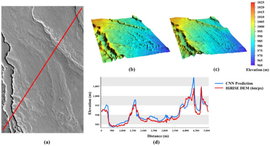
Figure 8.
Gully 3D reconstruction results: (a) CTX image; (b) 3D surface generated by the proposed method; (c) 3D surface generated by a HiRISE DEM; (d) Comparison of selected profiles.
Cones of various sizes are present on the Martian surface, as shown in Figure 9. Most of these cones had a diameter larger than 10 pixels and were successfully reconstructed. The profiles in Figure 9d show that the basic cone structures were recovered, and the elevations were close to those of the ground truth. Among several big cones, there were series of connected small cones that were continuously reconstructed. The RMSE value for this dataset was 4.02 m.
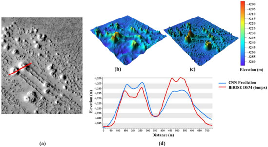
Figure 9.
Cone 3D reconstruction results: (a) CTX image; (b) 3D surface generated by the proposed method; (c) 3D surface generated by a HiRISE DEM; (d) Comparison of selected profiles.
Figure 10 shows several craters of different diameters and depths, which reveals that deep, large craters were well reconstructed, although they were shallower than the ground-truth craters. The crater reconstructions with similar pixel values in darker terrain were poorer in quality than deeper crater reconstructions. In addition, the edges along the illumination direction of some craters were a little higher than those along other directions. Noise on the terrain surface was removed along with some topographical details, so the prediction was smoother than the ground truth. The RMSE value of this dataset was approximately 6.32 m.
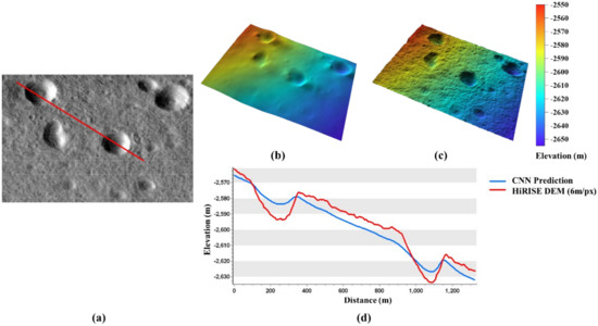
Figure 10.
3D reconstruction results of craters: (a) CTX image; (b) 3D surface generated by the proposed method; (c) 3D surface generated by HiRISE DEM; (d) Comparison of selected profiles.
4.3. Results of Different Low-Resolution DEMs
Publicly available DEMs of the Martian surface have various spatial resolutions. To quantify the effects of using DEMs with different spatial resolutions as constraints, we introduced the CTX DEM, HRSC DEM, and MOLA DEM into the experiment. All DEMs were adjusted to have the same mean elevation for comparison. The HiRISE DEM was down-sampled to 6 m/pixel and used as the ground truth for comparison. Difference maps were generated to evaluate the performance of the proposed method. Table 4 presents details of the data used.
Table 4.
Information on the images and low-resolution DEMs.
Figure 11 presents our 3D reconstruction results using variable low-resolution DEMs as constraints. The gully was successfully reconstructed with high accuracy, and some small features are also visible. Different low-resolution DEM reconstructions show similar topographical details, but different global information, which implies that the proposed method can be applied to refine the resolution of existing devices that are used to create DEMs. The difference maps in Figure 12 confirm that our method can refine low-resolution DEMs to the same resolution as the input image, with good accuracy. Table 5 lists the RMSE results.
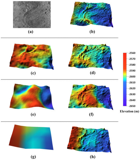
Figure 11.
3D reconstruction results using different low-resolution DEMs as constraints: (a) CTX image (6 m/pixel); (b) 3D surface generated by a HiRISE DEM (6 m/pixel); (c) 3D surface generated by a CTX DEM (20 m/pixel); (d) 3D surface generated by a refined CTX DEM (6 m/pixel); (e) 3D surface generated by a HRSC DEM (52 m/pixel); (f) 3D surface generated by a refined HRSC DEM (6 m/pixel); (g) MOLA DEM (463 m/pixel); (h) 3D surface generated by a refined MOLA DEM (6 m/pixel).
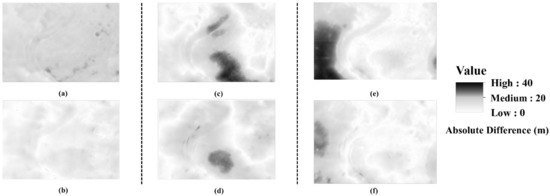
Figure 12.
Comparison of difference maps obtained with the HiRISE DEM (6 m/pixel): (a) Difference map of an original CTX DEM (20 m/pixel); (b) Difference map of the refined CTX DEM (6 m/pixel); (c) Difference map of the HRSC DEM (52 m/pixel); (d) Difference map of the refined HRSC DEM (6 m/pixel); (e) Difference map of the MOLA DEM (463 m/pixel); (f) Difference map of the refined MOLA DEM (6 m/pixel).
Table 5.
RMSE results for DEMs of different resolutions and for our predictions.
5. Discussion
It should be noted that two datasets were used in the proposed training process. A synthetic dataset was used to initialize the network parameters, and a real-world dataset was used to fine-tune those parameters. This strategy is based on the fact that the quality of CTX images varies, with some contaminated by weather, camera noise, and variable illumination. Thus, a network that can filter noise and recognize correct topographical information from images is required. However, artificially generated datasets contain no noise, which means that the network tends to assume that any change in pixel values corresponds to a topographic change that should be detected and included in the final product. This phenomenon worsens if the network is trained for a long time using synthetic data. Thus, the training strategy must balance the numbers of epochs using the synthetic and real-world datasets based on the noise level of the images. In addition, to generate DEMs with abundant surface details, the quality levels of the images and corresponding DEMs are equally important. If changes in the pixel values in the images do not correspond with changes in the DEM labels, the network recognizes the changes as noise and removes them in subsequent processes. Therefore, the key to dataset quality is not spatial resolution but excellent correspondence between training samples and labels.
Some mosaicked boundaries in the results may contain slightly visible seamlines, for which there are several possible reasons. For example, scale estimation based on linear regression is not optimally accurate for all images, which creates scale uncertainty in the final product. In addition, standard deviations of predictions are required to estimate possible elevation differences. However, the accuracy of 3D reconstruction results affects the magnitude of standard deviations, thereby introducing more uncertainty. Seamlines exist in areas with sharp elevation changes, whereas they are almost invisible in smooth terrain. A possible solution to this problem is to identify existing high-resolution DEMs of the proposed area and perform a linear regression to calculate the parameters in this specific area, as our statistics are based on global data of the Martian surface. This is because these global statistics are based on 8-bit CTX images with gray values ranging from 0 to 255; thus, introducing images with different gray value ranges or image formats may lead to failure to recover the correct scales. Some prerequisites should also be noted. The proposed scale recovery method assumes that the low-resolution DEMs used for refining the parameters contain sufficient topographical information. The other prerequisite is that noise such as shadow and albedo variation in the image should be small and cannot be dominant in the image, so that noise can be eliminated as outliers. In addition, the performance of the proposed scale recovery method also depends on the consistency of photometric, illumination, and atmospheric conditions in the dataset. A more internally consistent dataset would result in more accurate scale recovery parameters while limiting its applicable range. On the other hand, a more diverse dataset applies to a wider range of imaging conditions, but the accuracy of the recovery parameters decreases (e.g., the dot dispersion in Figure 5) due to variations in the photometric, illumination, and atmospheric conditions of the images. Therefore, it is believed that a more robust scale recovery method will further improve the proposed CNN-based approach. Nevertheless, the method worked well in our experimental analysis. For images with photometric and imaging conditions significantly different from those of the training dataset, a dataset more consistent with these images may be needed to tune the CNN model. Research from photoclinometry, or SfS, has confirmed that gray images only have a strong relationship with gradient changes along the illumination direction of terrain elevations [37,38]. Gradients only contain relative elevation information and, when revealed in images, are reliable only in a local range. If other DEMs are not introduced into our proposed method, although the final products correctly reconstruct local topography, they do not indicate global tendencies. This means that while on the global scale an overall surface may be flat, without any slopes, topographical details occur on the local scale. The reconstruction results for sand dunes, gullies, and craters all include global slopes of the terrain, which cannot be recovered by the CNN and must be provided by other DEMs.
6. Conclusions
In this study, we developed a novel CNN-based approach for high-resolution 3D reconstruction of the Martian surface from single imagery. A scale recovery method based on dataset statistics was developed and successfully applied using this framework. The experimental results validated the performance of our proposed method. High-resolution DEMs were reconstructed successfully from images of the same resolution.
The degree of geometric accuracy achieved is also promising, with RMSE values ranging from 2.1 m to 12.2 m, corresponding to approximately 0.5 to 2 pixels in the image space (considering a 6 m/pixel resolution for the input CTX imagery). The proposed method was also able to enrich the topographical details and improve the overall accuracy of existing DEM tools, i.e., the MOLA and HRSC DEMs. As there are few high-resolution stereo (e.g., HiRISE or CTX) images of the Martian surface, and as low-resolution DEMs are globally available (e.g., from MOLA), the proposed CNN-based method shows great potential for generating high-resolution DEMs with good accuracy from single images.
Our future work will focus on improving the robustness of the scale recovery algorithm, as well as the accuracy and details of the 3D reconstruction. It is also important to test different photometric models to present the Martian surface. For example, using the lunar-Lambert model instead of the Lommel–Seeliger model might be better to separate albedo from shading. Comparing and integrating the CNN-based method with existing methods such as photoclinometry or SfS for 3D reconstruction of the Martian surface is also of interest.
Author Contributions
Conceptualization and supervision, B.W.; methodology, Z.C. and W.C.L.; software and validation, Z.C.; Writing—original draft, Z.C.; Writing—review and editing, B.W. All authors have read and agreed to the published version of the manuscript.
Funding
This work was funded by grants from the Research Grants Council of Hong Kong (Project No: R5043-19; Project No: G-PolyU505/18; Project No: PolyU15210520). The work was also supported by a grant from Beijing Municipal Science and Technology Commission (Project No: Z191100004319001).
Institutional Review Board Statement
Not applicable.
Informed Consent Statement
Not applicable.
Data Availability Statement
Publicly available datasets were analyzed in this study. The datasets can be found here: https://ode.rsl.wustl.edu/mars/.
Acknowledgments
The authors would like to thank all those who worked on the archive of the datasets to make them publicly available.
Conflicts of Interest
The authors declare no conflict of interest.
References
- De Rosa, D.; Bussey, B.; Cahill, J.T.; Lutz, T.; Crawford, I.A.; Hackwill, T.; van Gasselt, S.; Neukum, G.; Witte, L.; McGovern, A.; et al. Characterisation of potential landing sites for the European Space Agency’s Lunar Lander project. Planet. Space Sci. 2012, 74, 224–246. [Google Scholar] [CrossRef]
- Wu, B.; Li, F.; Ye, L.; Qiao, S.; Huang, J.; Wu, X.; Zhang, H. Topographic modeling and analysis of the landing site of Chang’E-3 on the Moon. Earth Planet. Sci. Lett. 2014, 405, 257–273. [Google Scholar] [CrossRef]
- Wu, B.; Li, F.; Hu, H.; Zhao, Y.; Wang, Y.; Xiao, P.; Li, Y.; Liu, W.C.; Chen, L.; Ge, X.; et al. Topographic and geomorphological mapping and analysis of the Chang’E-4 landing site on the far side of the Moon. Photogramm. Eng. Remote Sens. 2020, 86, 247–258. [Google Scholar] [CrossRef]
- Hynek, B.M.; Beach, M.; Hoke, M.R.T. Updated global map of Martian valley networks and implications for climate and hydrologic processes. J. Geophys. Res. Planets 2010, 115. [Google Scholar] [CrossRef]
- Brooker, L.M.; Balme, M.R.; Conway, S.J.; Hagermann, A.; Barrett, A.M.; Collins, G.S.; Soare, R.J. Clastic polygonal networks around Lyot crater, Mars: Possible formation mechanisms from morphometric analysis. Icarus 2018, 302, 386–406. [Google Scholar] [CrossRef]
- Williams, R.M.E.; Weitz, C.M. Reconstructing the aqueous history within the southwestern Melas basin, Mars: Clues from stratigraphic and morphometric analyses of fans. Icarus 2014, 242, 19–37. [Google Scholar] [CrossRef]
- Head, J.W.; Fassett, C.I.; Kadish, S.J.; Smith, D.E.; Zuber, M.T.; Neumann, G.A.; Mazarico, E. Global distribution of large lunar craters: Implications for resurfacing and impactor populations. Science 2010, 329, 1504–1507. [Google Scholar] [CrossRef] [PubMed]
- Smith, D.E.; Zuber, M.T.; Frey, H.V.; Garvin, J.B.; Head, J.W.; Muhleman, D.O.; Pettengill, G.H.; Phillips, R.J.; Solomon, S.C.; Zwally, H.J.; et al. Mars Orbiter Laser Altimeter: Experiment summary after the first year of global mapping of Mars. J. Geophys. Res. Planets 2001, 106, 23689–23722. [Google Scholar] [CrossRef]
- Jaumann, R.; Neukum, G.; Behnke, T.; Duxbury, T.C.; Eichentopf, K.; Flohrer, J.; Gasselt, S.V.; Giese, B.; Gwinner, K.; Hauber, E.; et al. The high-resolution stereo camera (HRSC) experiment on Mars express: Instrument aspects and experiment conduct from interplanetary cruise through the nominal mission. Planet. Space Sci. 2007, 55, 928–952. [Google Scholar] [CrossRef]
- Kim, J.-R.; Lin, S.-Y.; Choi, Y.-S.; Kim, Y.-H. Toward generalized planetary stereo analysis scheme—prototype implementation with multi-resolution Martian stereo imagery. Earth Planets Space 2013, 65, 799–809. [Google Scholar] [CrossRef]
- McEwen, A.S.; Banks, M.E.; Baugh, N.; Becker, K.; Boyd, A.; Bergstrom, J.W.; Beyer, R.A.; Bortolini, E.; Bridges, N.T.; Byrne, S.; et al. The high resolution imaging science experiment (HiRISE) during MRO’s primary science phase (PSP). Icarus 2010, 205, 2–37. [Google Scholar] [CrossRef]
- Smith, D.E.; Zuber, M.T.; Jackson, G.B.; Cavanaugh, J.F.; Neumann, G.A.; Riris, H.; Sun, X.; Zellar, R.S.; Coltharp, C.; Connelly, J.; et al. The Lunar Orbiter Laser Altimeter investigation on the Lunar Reconnaissance Orbiter mission. Space Sci. Rev. 2010, 150, 209–241. [Google Scholar] [CrossRef]
- Wu, B.; Hu, H.; Guo, J. Integration of Chang’E-2 imagery and LRO laser altimeter data with a combined block adjustment for precision lunar topographic modeling. Earth Planet. Sci. Lett. 2014, 391, 1–15. [Google Scholar] [CrossRef]
- Zhu, Q.; Zhang, Y.; Wu, B.; Zhang, Y. Multiple close-range image matching based on a self-adaptive triangle constraint. Photogramm. Rec. 2010, 25, 437–453. [Google Scholar] [CrossRef]
- Zurek, R.W.; Smrekar, S.E. An overview of the Mars Reconnaissance Orbiter (MRO) science mission. J. Geophys. Res. Planets 2007, 112. [Google Scholar] [CrossRef]
- Liu, W.C.; Wu, B.; Wöhler, C. Effects of illumination differences on photometric stereo shape-and-albedo-from-shading for precision lunar surface reconstruction. ISPRS J. Photogramm. Remote Sens. 2018, 136, 58–72. [Google Scholar] [CrossRef]
- Wu, B.; Liu, W.C.; Grumpe, A.; Wöhler, C. Construction of pixel-level resolution DEMs from monocular images by shape and albedo from shading constrained with low-resolution DEM. ISPRS J. Photogramm. Remote Sens. 2018, 140, 3–19. [Google Scholar] [CrossRef]
- Grumpe, A.; Belkhir, F.; Wöhler, C. Construction of lunar DEMs based on reflectance modelling. Adv. Space Res. 2014, 53, 1735–1767. [Google Scholar] [CrossRef]
- Liu, W.C.; Wu, B. An integrated photogrammetric and photoclinometric approach for illumination-invariant pixel-resolution 3D mapping of the lunar surface. ISPRS J. Photogramm. Remote Sens. 2020, 159, 153–168. [Google Scholar] [CrossRef]
- Yosinski, J.; Clune, J.; Nguyen, A.; Fuchs, T.; Lipson, H. Understanding neural networks through deep visualization. arXiv 2015, arXiv:1506.06579. [Google Scholar]
- Laina, I.; Rupprecht, C.; Belagiannis, V.; Tombari, F.; Navab, N. Deeper Depth Prediction with Fully Convolutional Residual Networks. In Proceedings of the 2016 Fourth International Conference on 3D Vision (3DV), Stanford, CA, USA, 25–28 October 2016; pp. 239–248. [Google Scholar]
- Eigen, D.; Puhrsch, C.; Fergus, R. Depth map prediction from a single image using a multi-scale deep network. In Advances in Neural Information Processing Systems 27; Ghahramani, Z., Welling, M., Cortes, C., Lawrence, N.D., Weinberger, K.Q., Eds.; Curran Associates, Inc.: Red Hook, NY, USA, 2014; pp. 2366–2374. [Google Scholar]
- Cao, Y.; Wu, Z.; Shen, C. Estimating Depth from monocular images as classification using deep fully convolutional residual networks. IEEE Trans. Circuits Syst. Video Technol. 2018, 28, 3174–3182. [Google Scholar] [CrossRef]
- Eigen, D.; Fergus, R. Predicting depth, surface normals and semantic labels with a common multi-scale convolutional architecture. In Proceedings of the 2015 IEEE International Conference on Computer Vision (ICCV), Santiago, Chile, 7–13 December 2015; IEEE: New York, NY, USA, 2015; pp. 2650–2658. [Google Scholar]
- Ma, F.; Karaman, S. Sparse-to-dense: Depth prediction from sparse depth samples and a single image. In Proceedings of the 2018 IEEE International Conference on Robotics and Automation (ICRA), Brisbane, Australia, 21–25 May 2018; pp. 4796–4803. [Google Scholar]
- Fangmin, L.; Ke, C.; Xinhua, L. 3D face reconstruction based on convolutional neural network. In Proceedings of the 2017 10th International Conference on Intelligent Computation Technology and Automation (ICICTA), Changsha, China, 9–10 October 2017; pp. 71–74. [Google Scholar]
- Jackson, A.S.; Bulat, A.; Argyriou, V.; Tzimiropoulos, G. Large pose 3D face reconstruction from a single image via direct volumetric CNN regression. In Proceedings of the International Conference on Computer Vision, Venice, Italy, 22–29 October 2017; pp. 1031–1039. [Google Scholar]
- Chinaev, N.; Chigorin, A.; Laptev, I. MobileFace: 3D Face reconstruction with efficient CNN regression. In Proceedings of the European Conference on Computer Vision (ECCV) Workshops, Munich, Germany, 8–14 September 2018. [Google Scholar]
- Sengupta, S.; Kanazawa, A.; Castillo, C.D.; Jacobs, D.W. SfSNet: Learning shape, reflectance and illuminance of faces ‘in the wild’. In Proceedings of the IEEE Conference on Computer Vision and Pattern Recognition (CVPR), Salt Lake City, UT, USA, 18–23 June 2018; pp. 6296–6305. [Google Scholar]
- Guo, Y.; Zhang, J.; Cai, J.; Jiang, B.; Zheng, J. CNN-based real-time dense face reconstruction with inverse-rendered photo-realistic face images. IEEE Trans. Pattern Anal. Mach. Intell. 2019, 41, 1294–1307. [Google Scholar] [CrossRef] [PubMed]
- Chen, Z.; Wu, B.; Liu, W.C. Deep learning for 3D reconstruction of the Martian surface using monocular images: A first glance. ISPRS Int. Arch. Photogramm. Remote Sens. Spat. Inf. Sci. 2020, XLIII-B3-2020, 1111–1116. [Google Scholar] [CrossRef]
- Beyer, R.A.; Alexandrov, O.; McMichael, S. The Ames Stereo Pipeline: NASA’s open source software for deriving and processing terrain data. J. Geophys. Res. Planets 2017, 5, 537–548. [Google Scholar] [CrossRef]
- Beyer, R.A.; Kirk, R.L. Meter-scale slopes of candidate MSL landing sites from point photoclinometry. Space Sci. Rev. 2012, 170, 775–791. [Google Scholar] [CrossRef]
- Beyer, R.A.; McEwen, A.S.; Kirk, R.L. Meter-scale slopes of candidate MER landing sites from point photoclinometry. J. Geophys. Res. Planets 2003, 108. [Google Scholar] [CrossRef]
- Rouy, E.; Tourin, A. A viscosity solutions approach to shape-from-shading. SIAM J. Numer. Anal. 1992, 29, 867–884. [Google Scholar] [CrossRef]
- Oliensis, J.; Dupuis, P. A global algorithm for shape from shading. In Proceedings of the 1993 (4th) International Conference on Computer Vision, Berlin, Germany, 11–14 May 1993; IEEE Computer Society Press: Piscataway, NJ, USA, 1993; pp. 692–701. [Google Scholar]
- Horn, B.K.P. Obtaining shape from shading information. In The Psychology of Computer Vision; McGraw-Hill: New York, NY, USA, 1975; Chapter 4; pp. 115–155. [Google Scholar]
- Falcone, M.; Sagona, M. An algorithm for the global solution of the shape-from-shading model. In Image Analysis and Processing, Proceedings of the ICIAP: International Conference on Image Analysis and Processing, Florence, Italy, 17–19 September 1997; Del Bimbo, A., Ed.; Springer: Berlin/Heidelberg, Germany, 1997; pp. 596–603. [Google Scholar]
- Camilli, F.; Grüne, L. Numerical approximation of the maximal solutions for a class of degenerate Hamilton-Jacobi equations. SIAM J. Numer. Anal. 2000, 38, 1540–1560. [Google Scholar] [CrossRef]
- Kirk, R.L.I. Thermal Evolution of Ganymede and Implications for Surface Features. II. Magnetohydrodynamic Constraints on Deep Zonal Flow in the Giant Planets. III. A Fast Finite-Element Algorithm for Two-Dimensional Photoclinometry. Ph.D. Thesis, California Institute of Technology, Pasadena, CA, USA, 1987. [Google Scholar]
- Horn, B.K.P. Height and gradient from shading. Int. J. Comput. Vis. 1990, 5, 37–75. [Google Scholar] [CrossRef]
- Barron, J.T.; Malik, J. Shape, albedo, and illumination from a single image of an unknown object. In Proceedings of the 2012 IEEE Conference on Computer Vision and Pattern Recognition, Providence, RI, USA, 16–21 June 2012; IEEE: New York, NY, USA, 2012; pp. 334–341. [Google Scholar]
- Barron, J.T.; Malik, J. High-frequency shape and albedo from shading using natural image statistics. In Proceedings of the CVPR 2011, Colorado Springs, CO, USA, 20–25 June 2011; IEEE: New York, NY, USA, 2011; pp. 2521–2528. [Google Scholar]
- Tenthoff, M.; Wohlfarth, K.; Wöhler, C. High resolution digital terrain models of Mercury. Remote Sens. 2020, 12, 3989. [Google Scholar] [CrossRef]
- Fu, K.; Peng, J.; He, Q.; Zhang, H. Single image 3D object reconstruction based on deep learning: A review. Multimed. Tools Appl. 2021, 80, 463–498. [Google Scholar] [CrossRef]
- Fan, H.; Su, H.; Guibas, L. A point set generation network for 3D object reconstruction from a single image. In Proceedings of the 2017 IEEE Conference on Computer Vision and Pattern Recognition (CVPR), Honolulu, HI, USA, 21–26 July 2017; pp. 2463–2471. [Google Scholar]
- Xia, Y.; Wang, C.; Xu, Y.; Zang, Y.; Liu, W.; Li, J.; Stilla, U. RealPoint3D: Generating 3D point clouds from a single image of complex scenarios. Remote Sens. 2019, 11, 2644. [Google Scholar] [CrossRef]
- Pontes, J.K.; Kong, C.; Sridharan, S.; Lucey, S.; Eriksson, A.; Fookes, C. Image2Mesh: A learning framework for single image 3D reconstruction. In Computer Vision—ACCV 2018, Proceedings of the 14th Asian Conference on Computer Vision, Perth, Australia, 2–6 December 2018; Jawahar, C.V., Li, H., Mori, G., Schindler, K., Eds.; Springer International Publishing: Cham, Switzerland, 2019; pp. 365–381. [Google Scholar]
- Hapke, B. Theory of Reflectance and Emittance Spectroscopy; Cambridge University Press: Cambridge, UK, 2012; ISBN 978-1-139-21750-7. [Google Scholar]
- Szegedy, C.; Ioffe, S.; Vanhoucke, V.; Alemi, A.A. Inception-v4, Inception-ResNet and the impact of residual connections on learning. In Proceedings of the Thirty-First AAAI Conference on Artificial Intelligence, San Francisco, CA, USA, 4–9 February 2017; pp. 4278–4284. [Google Scholar]
- Ronneberger, O.; Fischer, P.; Brox, T. U-Net: Convolutional networks for biomedical image segmentation. In Medical Image Computing and Computer-Assisted Intervention—MICCAI 2015, Proceedings of the 18th International Conference, Munich, Germany, 5–9 October 2015; Navab, N., Hornegger, J., Wells, W.M., Frangi, A.F., Eds.; Springer International Publishing: Cham, Switzerland, 2015; pp. 234–241. [Google Scholar]
- Odena, A.; Dumoulin, V.; Olah, C. Deconvolution and checkerboard artifacts. Distill 2016, 1, e3. [Google Scholar] [CrossRef]
- Glorot, X.; Bordes, A.; Bengio, Y. Deep sparse rectifier neural networks. In Proceedings of the Fourteenth International Conference on Artificial Intelligence and Statistics, JMLR Workshop and Conference Proceedings, Fort Lauderdale, FL, USA, 11–13 April 2011; pp. 315–323. [Google Scholar]
- Jin, X.; Xu, C.; Feng, J.; Wei, Y.; Xiong, J.; Yan, S. Deep learning with S-shaped rectified linear activation units. arXiv 2015, arXiv:1512.07030. [Google Scholar]
- Abadi, M.; Barham, P.; Chen, J.; Chen, Z.; Davis, A.; Dean, J.; Devin, M.; Ghemawat, S.; Irving, G.; Isard, M.; et al. TensorFlow: A system for large-scale machine learning. In Proceedings of the 12th USENIX Symposium on Operating Systems Design and Implementation (OSDI ’16), Savannah, GA, USA, 2–4 November 2016; pp. 265–283. [Google Scholar]
- Kingma, D.P.; Ba, J. Adam: A method for stochastic optimization. arXiv 2017, arXiv:1412.6980. [Google Scholar]
- Choi, S.; Kim, T.; Yu, W. Performance evaluation of RANSAC Family. In Proceedings of the British Machine Vision Conference 2009, London, UK, 7–10 September 2009; pp. 81.1–81.12. [Google Scholar]
- Wang, Z.; Bovik, A.C.; Sheikh, H.R.; Simoncelli, E.P. Image quality assessment: From error visibility to structural similarity. IEEE Trans. Image Process. 2004, 13, 600–612. [Google Scholar] [CrossRef] [PubMed]


Publisher’s Note: MDPI stays neutral with regard to jurisdictional claims in published maps and institutional affiliations. |
© 2021 by the authors. Licensee MDPI, Basel, Switzerland. This article is an open access article distributed under the terms and conditions of the Creative Commons Attribution (CC BY) license (http://creativecommons.org/licenses/by/4.0/).