Abstract
The supply–demand relationship of urban public service facilities is the key to measuring a city’s service level and quality, and a balanced supply–demand relationship is an important indicator that reflects the optimal allocation of resources. To address the problem presented by the unbalanced distribution of educational resources, this paper proposes a dynamic Voronoi diagram algorithm with conditional constraints (CCDV). The CCDV method uses the Voronoi diagram to divide the plane so that the distance from any position in each polygon to the point is shorter than the distance from the polygon to the other points. In addition, it can overcome the disadvantage presented by the Voronoi diagram’s inability to use the nonspatial attributes of the point set to precisely constrain the boundary range; the CCDV method can dynamically plan and allocate according to the school’s capacity and the number of students in the coverage area to maintain a balance between supply and demand and achieve the optimal distribution effect. By taking the division of school districts in the Bao’an District, Shenzhen, as an example, the method is used to obtain a school district that matches the capacity of each school, and the relative error between supply and demand fluctuates only from −0.1~0.15. According to the spatial distribution relationship between schools and residential areas in the division results, the schools in the Bao’an District currently have an unbalanced distribution in some areas. A comparison with the existing school district division results shows that the school district division method proposed in this paper has advantages. Through a comprehensive analysis of the accessibility of public facilities and of the balance of supply and demand, it is shown that school districts based on the CCDV method can provide a reference for the optimal layout of schools and school districts.
1. Introduction
As the level of urbanization increases, cities are rapidly expanding, their populations are growing, and the demand and requirements for public service facilities are gradually increasing. However, the insufficient construction of public service facilities and low standards are generating problems such as a lack of coordination between facility construction and urban space expansion that results in an imbalance between facility supply and demand [1,2,3]. The fundamental contradiction between the construction of urban public facilities and the areas where services are needed is the imbalance between supply and demand: it is particularly important that existing resources be reasonably allocated to ensure such a balance.
Public service facilities specifically include education, medical and health, culture, sports, transportation, social welfare, and security facilities [4]. In recent years, a belief in the “equalization of basic public service facilities” has gradually taken root, and educational equity has become a common concern across all sectors of society [5,6]. Urban school districts are a manifestation of the balanced distribution of urban basic education resources. In China, elementary school students are sent to schools in their school district based on the principle of nearest enrollment [7,8]. However, with the continuous increase in the urban population, the number of school-age children is also increasing. The capacity in public primary schools in large and medium-sized cities is limited, which means the nearest school is often unable to enroll all school-age children in the surrounding area. This makes it difficult for families to enroll at a nearby school and also makes the phenomenon of choosing across schools universal. It is thus worth studying this space optimization problem to determine how to dynamically divide school districts or automatically allocate places, so as to ensure that as many students as possible can enroll in a nearby school.
The problem of school district division has a certain degree of complexity and has always attracted academic attention. Therefore, many scholars have conducted research to determine the exact or approximate solution to achieve optimal enrollment. The school district division methods mainly focus on mathematical models, the Geographic Information System (GIS), and the heuristic algorithm.
References [9,10,11,12,13] applied different the mathematical models to study the division of school districts. They constructed a variety of linear constraint models for the shortest distance between students and the school and the lowest transportation cost. However, the mathematical model approach is mainly a simple statistical comparison of data; these models are unable to consider the problem of spatial layout, most involve NP-hard problems, and it is difficult to obtain stable and effective solutions [14,15]. References [16,17,18,19] mainly applied GIS methods such as the buffer analysis method, road network distance analysis method, and Thiessen polygon division method. Caro et al. [16] and Kong [18] based on the principles of the shortest total enrollment distance and the continuity of the division area, using the buffer analysis method and road network analysis distance method to develop the optimal school district division tool. However, they can hardly cover all areas continuously. References [19,20,21,22,23] took continuity and compactness as constraints, and studied the model of school district division based on Thiessen polygon and network analysis. Although the Thiessen polygon method can cover all the space and minimize the traffic cost, it is difficult to take into account the contradiction between supply and demand or between schools and residents. In recent years, an increasing number of problems with complex features have appeared, and a single heuristic algorithm may be insufficient to address these challenges. Therefore, researchers [24,25,26] have started studying hybrid algorithms, that is, integrating two or more heuristic algorithms to solve the problem of school district division. Although these intelligent optimization algorithms can obtain high-quality solutions through continuous search and optimization, the computational complexity of the algorithms is high, and it is easy for them to fall into the local optimum. The most important thing is that it is difficult for them to simultaneously consider the spatial location and attribute constraints of data.
Scholars have conducted sufficient research on accessibility assessment methods. Luo and Wang [27] proposed a two-step floating catchment area (2SFCA) method when studying the accessibility of medical facilities, which is a more effective accessibility assessment method. This method uses a two-step floating search method based on service supply points and service demand points to calculate the accessibility of an area, which alleviates the problem of imbalance between supply and demand of service facilities. However, scholars found that the 2SFCA method sets a single search range for all service supply points and service demand points. The service supply point can only serve the demand points within the range and cannot provide services for the demand points outside the range, and it is believed that the accessibility of people within the service range is equal [28,29]. In response to these problems, scholars have carried out improved research based on the 2SFCA method. Luo and Qi [28] proposed the enhanced two-step floating catchment area method (E2SFCA) method. They think that people do not mind the difference in transit time within a few minutes when enjoying service facilities. Therefore, the distance decay within a period of time (for example, 0–10 min) is not serious, and a fixed decay coefficient can be used to express the decaying rules with distance. However, in the E2SFCA method, how to set the weight coefficient of distance decay has become a new problem. Luo and Whippo [30] believed that according to the different spatial distribution of service supply points and population, different areas should adopt different service ranges, so they proposed an improved 2SFCA method with variable service ranges. This method can solve the problem that service supply points cannot form a supply scale or service demand points cannot obtain services, which is caused by the scattered distribution of service supply points or service demand points. However, the setting of the search range threshold for service supply points and service demand points is also subjective [31]. In addition, scholars have proposed different accessibility assessment methods from the aspects of competitiveness of service supply points [32], differences in travel modes [33], and integration of multiple data [34].
From the perspective of school district division, distance and the balance of supply and demand are important constraints in school district division [35,36,37,38,39,40]. Due to the uneven distribution of schools and the continuous growth of the population in the central areas of the city, the supply of degrees provided by some schools is less than demand, while the supply of degrees for some schools slightly exceeds demand, and the supply–demand relationship of urban public service facilities is the key to measuring a city’s service level and service quality. The balance of the supply–demand relationship is an important indicator that reflects the optimal allocation of resources. When considering distance accessibility factors, in order to reduce the subjectivity of parameter settings and automatically obtain a fairer range of school districts, this paper attempts to use the Thiessen polygon method in GIS to automatically divide the school district and combine the supply and demand factors to further optimize the school district.
This article explores an optimization strategy for school district division from the perspective of supply and demand balance and constructs an algorithm for the dynamic division of school districts. It can not only consider the distance cost, but also balance the school capacity and the number of school-age children in the school district as much as possible. Specifically, a dynamic Voronoi diagram partition method based on attribute constraints (CCDV) is proposed to try to balance the supply and demand of school resources. First, a Voronoi diagram is constructed based on each school to fully consider the distance factor. Second, based on the school capacity and the population of school-age children within the polygon range, the range of each polygon in the Voronoi diagram is recalculated to maximize the balance between supply and demand. Third, by taking the layout of primary schools in the Bao’an District, Shenzhen, as an example, and using the community as a spatial unit, the Voronoi diagram method is applied to evaluate the supply and demand status of primary schools in the Bao’an District and optimize the district layout. Finally, according to the results of comparative experiments, it is judged whether the CCDV method is beneficial to the balance of supply and demand of school degrees. The research and application of the CCDV method can provide a reference for the division of urban school districts, with a view to enhancing the scientific foundation, authority, and rationality of public service facility planning.
2. Dynamic Voronoi Method Based on Conditional Constraints (CCDV)
Thiessen polygons are also called Voronoi diagrams, which are named after George Voronoi. They are a set of continuous polygons composed of vertical bisectors that connect two adjacent points. The distance from any point in a Thiessen polygon to the control points that constitute the polygon is less than the distance to the control points of other polygons [23,41]. Therefore, the Voronoi method can effectively solve the problem of nearby enrollment and divide an area into school districts with the minimum distance cost. Starting with school supply and school district demand, this paper proposes a dynamic Thiessen polygon elementary school district division strategy. It is based on the balance between supply and demand constraints to explore a suitable method of school district division.
The constrained dynamic Voronoi diagram method is based on the traditional Thiessen polygon algorithm. The traditional Thiessen polygon takes the point set as the initial data to divide the plane, so that the distance from any position in each polygon to the point (school) is shorter than the distance from the polygon to other points (schools). However, the Thiessen polygon only considers the distance constraint, the resulting polygon is fixed, and it cannot incorporate the nonspatial attributes of the point. Moreover, constraints cannot be set for the attribute relationship between other features within the polygon coverage and the initial point. Therefore, an improvement must be made on the basis of the Voronoi diagram method.
First, the dynamic Voronoi graph algorithm with constraints can use the distance constraint of the Voronoi graph to form the initial coverage of each school. This coverage ensures that the distance between each school and surrounding student resources is acceptable. Second, each school has a student capacity, so the number of school-age children within the initial polygon is calculated. Here, the community is used as a spatial unit to calculate the population of school-age children in the study area, but it can also be calculated in different unit types (such as grid, transportation analysis zone). When the school’s capacity limit is reached, the accumulation stops. All communities that participate in the statistics are regarded as the school district, and the Voronoi diagram is re-established for the remaining data, and the next round of calculation is performed. If the cumulative number of school-age children in a polygon does not reach the school’s capacity limit, then the search is expanded around the polygon by a certain step length until the school’s accommodation limit is reached, and it is then reaccumulated based on the expanded range. After repeated iterative calculations, when all schools or student sources are allocated, a spatially continuous school district is formed, and the number of students covered by the school district and the school’s capacity are balanced, that is, balance is achieved between the school’s supply and demand. Figure 1 shows the implementation process of the constrained dynamic Voronoi diagram (CCDV) method.
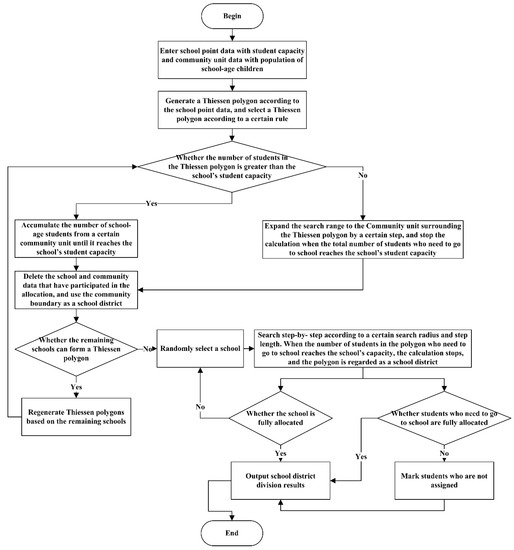
Figure 1.
Flow chart of the CCDV method.
The implementation steps of the CCDV method are as follows.
- (1)
- By taking the school’s spatial position as the reference point, use the Voronoi diagram algorithm to segment the plane where the school is located and ensure that the boundary of the generated Thiessen polygon can cover all areas with school-age students.
- (2)
- Calculate the center of gravity of each Thiessen polygon, and sort the centers of gravity from low to high in the order of longitude first and then latitude to form a fixed sequence of Thiessen polygons.
- (3)
- Select the first Thiessen polygon, assuming that the number of students in the school within the polygon is (i refers to a school). The total number of school-age children within the polygon is counted according to the community units covered by the polygon. First, calculate the center of gravity of each community, and sort the center of gravity from low to high in the order of longitude first and then latitude. Second, suppose that there are j community units in the range, and that the number of students represented by each unit is . Again, sequentially accumulate the number of school-age students in the area according to the order of the community’s center of gravity, that is, . Since it is generally impossible to guarantee that the number of students in a school zone is exactly equal to the school’s capacity, a floating range is set for the school’s capacity so that the number of students in each school zone will float within a certain range. Given the situation in Shenzhen, the school capacity range set in this article is . This parameter can be adjusted according to actual needs. If , then stop the iteration. M is the number of students assigned to the school, and all community units that participate in the iteration represent the area covered by the school district.
- (4)
- If all the community units in the polygon in the previous step cannot meet the stop condition after iterating, then this means that the number of students in the area is less than the number that the school can accommodate. Therefore, expand the search range. Setting too small a range will result in low search efficiency, and setting too large a range will cause the distance between students and the school to be too far, which is not conducive to the principle of nearby enrollment. To address this, the algorithm will gradually expand the search range to search for the optimal area. First, set an initial expansion range based on the original polygon boundary, which is 100 m in this article. Then, set a search step length, which in this article is 10 m, and the range will be gradually expanded on the basis of a 100 m range. When the total number of students in the search area is less than or equal to the number of students that the school can accommodate, the search stops. The polygon boundary is regarded as the new school district range.
- (5)
- Save the mapping relationship between the schools and community units that have been allocated. At the same time, remove the allocated schools and community units from the original data. Regenerate Thiessen polygons from the remaining school point data, and return to step (1) to start the next round of iterative calculations.
- (6)
- Since at least 3three points can form a Thiessen polygon, when iterating to the last two remaining schools, a polygon cannot be formed. Therefore, arbitrarily choose a school as the center, and follow the method in step (4) to expand the search range gradually. Stop the search when the total number of students in the search area is less than or equal to the number of students that the school can accommodate, and the polygon boundary is regarded as the new school district range. Since it is impossible to ensure that the number of people allocated each time is exactly equal to the school’s capacity, there may be a surplus of schools or students at the end of the allocation, that is, the supply of schools and the demand for schools of school-age students may be imbalanced. Therefore, in the calculation, it is necessary to determine whether the school and the students are all allocated. If the school is allocated, then the results of all school district divisions are output; if there are too many students, then the students who are not allocated to the school are marked, and the corresponding community is output.
As shown in Figure 2, if there are five schools (A, B, C, D, E) in the study area, including the number of students that the school can accommodate and the distribution of school-age children, the CCDV method is used to divide the school district. Firstly, establish the Thiessen polygon based on the school location, and then select one of the polygons to compare the number of students who need to go to school and the number of school-age children in the area. If the capacity of the school A is greater than the existing number of school-age children in the area, expand the polygonal range until the school capacity is less than or equal to the number of school-age children, as shown in Figure 2c. Complete the first school district division and regenerate the Thiessen polygons for the remaining schools. Secondly, select the school B for calculation and find that the number of school-age students in this area is already greater than the capacity of the school, so this area is the second school district. After completing the second iteration calculation, new Thiessen polygons are generated for the remaining schools. Then, iterative calculations are performed on the remaining schools in turn, until all schools are divided or all school-age children are allocated. Finally, the result of school district division is obtained, as shown in Figure 2e. The school D has a larger capacity and covers students who originally belonged to School E. Therefore, School E can cover students in more distant areas until it reaches its capacity. It is found from Figure 2 that although the CCDV method may increase some distance costs, it can maximize the supply–demand ratio of the school within a certain distance range. It is important to solve the problem that the number of school-age students is far greater than the capacity provided by the school. The application of this method can increase the utilization rate of educational facilities and minimize the difference between supply and demand.
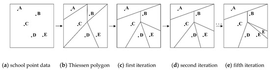
Figure 2.
Schematic diagram of the CCDV method for iterative division of school districts.
3. School District Division Experiment and Analysis
3.1. Experimental Area and Data Description
The object of this study is elementary schools as public service facilities. The service object of the elementary school is six- to 12-year-old children. Compared with middle and high school students, this younger group is characterized by a limited travel radius and walking as the primary travel mode. Facility accessibility is thus more sensitive for this group. Therefore, by taking the division of elementary school districts in the Bao’an District of Shenzhen as an example, the feasibility of the constraint-based dynamic Voronoi diagram method for the division of school districts is analyzed. According to the statistics of the Bao’an District, 137 primary schools can accommodate 140,743 students, and the population data of school-age children based on 4782 community units is 153,375. Community management urgently has been needed to improve grassroots social governance in recent years. The division of the community is based on the population, the road network, residential quarters, etc. At the same time, by considering the distance factor, it is consistent with the goal of enrolling in a nearby school. The distribution of elementary schools and the school-age population in the existing school districts in the Bao’an District are shown in Figure 3.
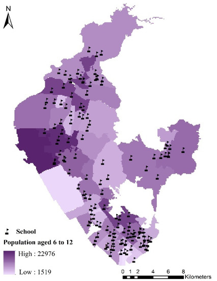
Figure 3.
Distribution of elementary schools and the school-age population in the existing school districts in the Bao’an District, Shenzhen.
Figure 3 shows that there are 46 school districts in the Bao’an District. There are large populations and a dense distribution of schools in the southwestern and southern parts of the district. The boundary of the school district is basically established by road networks. In other areas, it is most often divided by community administrative boundaries. In addition, there is a large gap between the number of students that the Bao’an District can support and the number of students who actually need to go to school. The official report of the Bao’an District confirms that there is an imbalance between supply and demand in the existing school district division.
Therefore, based on the supply and demand of the existing schools in the Bao’an District, Shenzhen, this paper applies the dynamic Voronoi diagram school district division method based on conditional constraints. Through the dynamic division of the school district, it is possible to achieve the maximum possible balance between the supply and demand for each school while enrolling more nearby students.
3.2. Experimental Results
The school point data with student capacity and the community unit data that contain the population of school-age children are substituted into the CCDV method. After repeated iterations, the school-age children in the community unit are allocated to various schools, and the result for the school district division in the Bao’an District, Shenzhen (Figure 4), is obtained. As shown in Figure 4, each color corresponds to an area covered by a school, and both the Voronoi method and the CCDV method are divided into 137 school districts, but the range of communities covered by each school is different. Because there are many areas, no legend is shown. The mapping relationship between the center of gravity of each school and the community unit is shown in Figure 5. The connection between each school and the community unit indicates that the students in the community are assigned to this school.
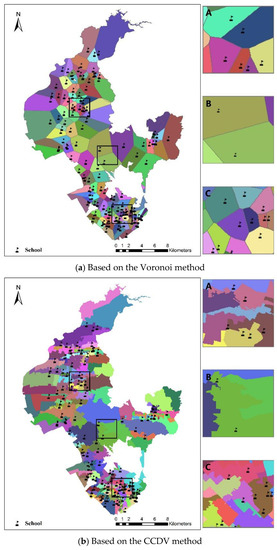
Figure 4.
School district division results.
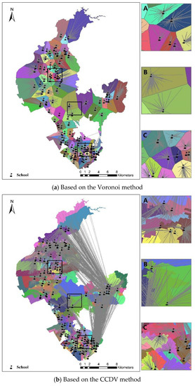
Figure 5.
Correspondence between schools and school-age children in the community unit.
By comparing (a) and (b) in Figure 4, we can see that the dynamic Voronoi method with constraints can not only consider the distance factor, but also allocate school-age children according to supply and demand conditions. The above view can be confirmed from the three enlarged areas of A, B, and C. Some school districts contain more than one school, indicating that the student capacity of schools in the area is greater than the demand, so the range of enrolling students can be expanded. In Figure 5, the community units covered by each school can be observed more clearly. Figure 5 also to a certain extent reflects the irrationality of the current layout of some schools in the Bao’an District. The community units that divide the Bao’an District into the northwest, middle, and south are basically clustered around the school, which can meet the school’s student capacity limit and the principle of nearby enrollment. However, the existence of reservoirs and forest parks in the central and eastern regions means that the population density is relatively sparse, while the distribution of schools is relatively dense, which causes an insufficient distribution of the number of students; thus, students must come from farther away, which results in the southeast area being assigned to these schools. In addition, because the northeastern part of the Bao’an District borders on another district (Guangming District), a concave administrative boundary is formed. Therefore, some schools in the northeast search other areas for students when the number enrolled do not reach the school supply capacity. It can be seen that a reasonable adjustment of the school layout can increase the convenience of enrollment and improve the balance of the distribution of educational resources.
3.3. Result Verification
By aiming at the problem of unbalanced resource allocation in the division of existing elementary schools in the Bao’an District and taking the supply and demand of the school district as the starting point, a dynamic Voronoi algorithm based on conditional constraints is proposed. The accessibility level and the supply and demand levels of the school district are calculated through a technical method of public service facility evaluation. The differences between the school districts generated by the improved algorithm, the school districts generated by the Voronoi algorithm, and the existing school districts are compared in terms of accessibility and the supply–demand balance. The rationality of using these different methods to divide school districts is then evaluated.
- (1)
- Accessibility
Accessibility is a key factor in evaluating the location of public service facilities. Accessibility measures the degree of effort required to reach the end point, and it can also indicate the potential for interaction between the start point and the end point. Regardless of the type of facility, balanced coverage is the goal when selecting the location of public service facilities. The public welfare characteristics of facilities and their social security functions determine that so-called balanced coverage should first be fair coverage, and balanced coverage is also more conducive to maximizing the utility of public service facilities.
The key factor in the layout of primary schools is to maximize their service levels, and the service utility of primary schools is largely determined by their accessibility. There are many ways to measure accessibility, including measurements of the affordability, acceptability, availability, and convenience of access to the service [42]. The research objects selected in this paper are public elementary schools. The geometric center of gravity of each elementary school is the supply point, the geometric center of the community unit is the demand point, and the Euclidean distance between these two points is used as a measure of accessibility. Because this article mainly focuses on differences in the distance between two points in different school district division methods, the linear distance between the center of gravity of the starting area is used for analysis. Table 1 shows the calculation of the different distances from the school to each community unit based on the existing school district, the school district based on the Voronoi division, and the school district based on the CCDV division.

Table 1.
Comparison of the distance to school for students in the school district based on different methods.
When the distance between the school and the residential area is smaller, the accessibility is better. It can be seen from Table 1 that the total distance to school for school-age children in the school district based on the Voronoi method is 1817.2 km less than the existing school district, the longest distance is 1.9 km less, the average school distance is 0.38 km less, and the optimization rate is 25.7%, which demonstrates that dividing school districts based on the Voronoi method is conducive to the implementation of the nearest admission policy. However, the distance to school for students in school districts based on the CCDV method is greater than the distance to school in the other two methods, especially the farthest distance, and the total distance is 365.8% greater than the total distance of the existing school district. This is mainly due to the unbalanced distribution of schools and students, which has led to schools searching for students farther away (as shown in Figure 4b); the average distance is only 37.2% greater than the average distance of the existing school district. This shows that if the distribution of schools can be reasonably adjusted, this method has certain advantages.
- (2)
- Supply and demand balance
The degree of supply and demand compares the supply of urban public facilities and the demand for these facilities from the external environment. By assessing the degree of supply and demand, contradictions between the supply and demand for public service facilities can be analyzed. Applying quantitative methods to evaluate the rationality of the distribution of urban public service facilities can provide references for realizing their effective spatial layout [43]. This article uses the relative error in the supply and demand of public service facilities to analyze the level provided by the facilities, and the formula is as follows.
Among the variables, K is the relative error between the supply and demand of students in a school zone (there are 46 school districts in the current plan and 137 school districts based on the Voronoi and CCDV methods), S is the number of students that can be accommodated by the schools in the school zone, and D is the total number of students that need to go to school in all community units in the school zone. Figure 6 shows the relative error of the school supply and demand in each school district based on the existing school district, the Voronoi-based school district, and the CCDV-based school district.

Figure 6.
The relative error of school supply and demand in the school districts based on different methods.
By using the relative error between the school capacity and the actual assigned number of students, the supply and demand status of the services provided by the schools in the area can be quantitatively analyzed and evaluated. When the relative error is positive, this means that supply is greater than demand; when it is negative, this means that demand is greater than supply. When the absolute value of the relative error is smaller, the supply and demand are more balanced. Figure 6 shows that the gap between the capacity of schools in the school district and the number of students that need to go to school calculated by the CCDV method is small and fluctuates from −0.1~0.15, which indicates that supply and demand are more balanced. The relative error of supply and demand calculated by the existing school district and the Voronoi method fluctuates greatly, especially for the school districts based on the Voronoi method. Although the Voronoi approach has advantages in accessibility, it performs poorly from the perspective of supply and demand balance.
The above results comprehensively show that the constrained dynamic Voronoi diagram method has a certain practical value in solving the problem of school district division. It can combine the school capacity and the number of school-age children in the analysis unit to accurately allocate the source of students to the corresponding school.
4. Conclusions
To address the problem of school district division, starting from school supply and school district demand, this paper proposes a school district division method based on the balance of supply and demand. The attribute constraints of school supply and school district demand are added to the traditional Voronoi diagram algorithm to form a constrained dynamic Voronoi diagram method. By taking the Bao’an District of Shenzhen as an example, this method is used to define elementary school districts. The feasibility and rationality of the method proposed in this paper are further verified by comparing the differences in the spatial accessibility of schools and the balance of supply and demand achieved by the different school district division methods.
When dividing school districts based on the CCDV method, the affiliation between schools and students is established, which shows that there is an imbalance between supply and demand in the distribution of existing school districts and schools. In the future, based on the methods mentioned in this article, the division of school districts and the spatial layout of schools can be reasonably adjusted. The CCDV method for dividing school districts can also take into account the issues of accessibility and the balance of supply and demand to achieve the optimal distribution effect. The method proposed in this paper reflects the intelligent automation of school district distribution and improves work efficiency. Comparing the existing school district with the school district based on the Voronoi method, it shows that the results of this article can help the education department accurately grasp the supply and demand situation of each school coverage area, which is conducive to promoting the rational allocation of urban education resources and has reference value for promoting the equalized development of urban education service facilities.
However, the CCDV method can only be used for single school district division at present. In areas where the allocation of educational resources is unbalanced and high-quality resources are concentrated in a few popular schools, a multi-slice division presents another option for sharing high-quality teaching resources and promoting educational equity. Future work aims to improve the method of this paper for application to the division of multiple school districts to meet actual needs more flexibly. Furthermore, the CCDV method will be tried in the allocation of facilities in other fields, such as medical and health, transportation, etc., so that the limited public facilities can serve more people from the perspective of supply and demand balance.
Author Contributions
Conceptualization: H.C.; methodology: H.C. and L.W.; validation: H.C., L.W., and S.H.; formal analysis: H.C. and L.W.; investigation: H.C.; data curation: H.C., S.H., and R.L.; writing—original draft preparation: H.C.; writing—review and editing: H.C. and L.W.; visualization: H.C. and S.H.; supervision: L.W.; project administration: L.W.; funding acquisition: L.W. All authors have read and agreed to the published version of the manuscript.
Funding
This study was financially supported by the National Natural Science Foundation of China (41871311), the National Key Research and Development Program (Grant No: 2017YFB0503600).
Data Availability Statement
The data presented in this study are available on request from the corresponding author. The data are not publicly available due to permissions.
Acknowledgments
The authors are thankful to the anonymous referees for their comments and suggestions that improved the quality of this paper.
Conflicts of Interest
The authors declare no conflict of interest.
References
- Setyono, D.; Cahyono, D.; Helmy, M. Measuring service capacity of public facilities based on supply aspect (Case study: Elementary school in Malang city). Procedia Soc. Behav. Sci. 2016, 227, 45–51. [Google Scholar] [CrossRef][Green Version]
- Jin, M.; Liu, L.; Tong, D.; Gong, Y.; Liu, Y. Evaluating the Spatial Accessibility and Distribution Balance of Multi-Level Medical Service Facilities. Int. J. Environ. Res. Public Health 2019, 16, 1150. [Google Scholar] [CrossRef]
- He, X.; Zhou, C.; Zhang, J.; Yuan, X. Using Wavelet Transforms to Fuse Nighttime Light Data and POI Big Data to Extract Urban Built-Up Areas. Remote Sens. 2020, 12, 3887. [Google Scholar] [CrossRef]
- Song, Z.; Chen, W.; Yuan, F.; Wang, L. Formulation of public facility location theory framework and literature review. Prog. Geogr. 2010, 29, 1499–1508. [Google Scholar]
- Zhang, J.; Ge, Z.; Luo, Z.; Sun, S. Research on equalized layout of urban and rural public facilities: A case study of educational facilities in Changzhou. City Plan. Rev. 2012, 36, 9–15. [Google Scholar]
- Mei, D.; Xiu, C.; Feng, X.; Wei, Y. Study of the School–Residence Spatial Relationship and the Characteristics of Travel-to-School Distance in Shenyang. Sustainability 2019, 11, 4432. [Google Scholar] [CrossRef]
- Li, J. A Positive Research on nearby enrollment at the stage of compulsory education. Res. Educ. Dev. 2007, 23, 39–43. [Google Scholar]
- Lu, N.; Huang, H. Examining the school choice phenomenon: Reflection on global context and local conditions. Res. Educ. Dev. 2009, 20, 1–6. [Google Scholar]
- Ernest, K. Mathematical analysis applied to school attendance areas. Socio Econ. Plan. Sci. 1968, 1, 465–475. [Google Scholar]
- Franklin, A.; Ernest, K. Computed school assignments in a large district. Oper. Res. 1973, 21, 413–426. [Google Scholar] [CrossRef]
- Heckmana, L.; Taylorb, H. School rezoning to achieve racial balance: A linear programming approach. Socio Econ. Plan. Sci. 1969, 3, 127–133. [Google Scholar] [CrossRef]
- Mckeown, P.; Workman, B. A study in using linear programming to assign students to schools. Interfaces 1976, 6, 96–101. [Google Scholar] [CrossRef]
- Taylor, R.; Vasu, M.; Causby, J. Intergrated planning for school and community: The case of Johnston county, North Carolina. Interfaces 1999, 29, 67–89. [Google Scholar] [CrossRef]
- Beheshtifar, S.; Alimoahmmadi, A. A multiobjective optimization approach for location-allocation of clinics. Int. Trans. Oper. Res. 2015, 22, 313–328. [Google Scholar] [CrossRef]
- He, Q. Study on Division of Primary School District in Beilin District, Xi’an City; Xian University of Architecture and Technology: Xi’an, China, 2018. [Google Scholar]
- Caro, F.; Shirabe, T.; Guignard, M.; Weintraub, A. School redistricting: Embedding GIS tools with integer programming. J. Oper. Res. Soc. 2004, 55, 836–849. [Google Scholar] [CrossRef]
- Novaes, A.G.N.; De Cursi, J.E.S.; Da Silva, A.C.L.; Souza, J.C. Solving continuous location-districting problems with Voronoi diagrams. Comput. Oper. Res. 2009, 36, 40–59. [Google Scholar] [CrossRef]
- Kong, Y. Optimal school allocation using GIS and linear programming. Geomat. Inf. Sci. Wuhan Univ. 2012, 37, 513–515. [Google Scholar]
- Tong, G.; Li, P.; Liu, Z.; Hu, Y. The GIS in Shenyang primary and secondary schools layout planning. Planners 2014, 30, 68–74. [Google Scholar]
- Chen, J.; Zhao, X.; Li, Z. An Algorithm for the Generation of Voronoi Diagrams on the Sphere Based on QTM. Photogramm. Eng. Rem. S. 2003, 69, 79–89. [Google Scholar] [CrossRef]
- Zhang, L.; Zhou, H. Research on Public Establishment Location Selection Based on the Voronoi Diagram in GIS. Comput. Eng. Appl. 2004, 40, 223–227. [Google Scholar]
- Okabe, A.; Satoh, T.; Furuta, T.; Suzuki, A.; Okano, K. Generalized network Voronoi diagrams: Concepts, computational methods, and applications. Int. J. Geogr. Inf. Sci. 2008, 22, 965–994. [Google Scholar] [CrossRef]
- Li, X.; Chen, J.; Zhao, L.; Guo, S.; Sun, L.; Zhao, X. Adaptive Distance-Weighted Voronoi Tessellation for Remote Sensing Image Segmentation. Remote Sens. 2020, 12, 4115. [Google Scholar] [CrossRef]
- Bong, C.; Wang, Y. A multiobjective hybrid metaheuristic approach for GIS-based spatial zoning model. J. Math. Model. Algorithms 2004, 3, 245–261. [Google Scholar]
- Kong, Y.; Zhu, Y.; Wang, Y. A hybrid metaheuristic algorithm for the school districting problem. Acta Geogr. Sin. 2017, 72, 256–268. [Google Scholar]
- Assad, A.; Deep, K. A hybrid harmony search and simulated annealing algorithm for continuous optimization. Inform. Sciences 2018, 450, 246–266. [Google Scholar]
- Luo, W.; Wang, F. Measures of Spatial Accessibility to Health Care in a GIS Environment: Synthesis and a Case Study in the Chicago Region. Environ. Plan. B Plan. Des. 2003, 30, 865–884. [Google Scholar] [CrossRef]
- Luo, W.; Qi, Y. An enhanced two-step floating catchment area (E2SFCA) method for measuring spatial accessibility to primary care physicians. Health Place 2009, 15, 1100–1107. [Google Scholar] [CrossRef]
- Mcgrail, M.; Humphreys, J. Measuring spatial accessibility to primary care in rural areas: Improving the effectiveness of the two-step floating catchment area method. Appl. Geogr. 2009, 29, 533–541. [Google Scholar] [CrossRef]
- Luo, W.; Whippo, T. Variable catchment sizes for the two-step floating catchment area (2SFCA) method. Health Place 2012, 18, 789–795. [Google Scholar] [CrossRef] [PubMed]
- Tao, Z.; Cheng, Y. Research progress of the two-step floating catchment area method and extensions. Prog. Geogr. 2016, 35, 589–599. [Google Scholar]
- Wan, N.; Zou, B.; Sternberg, T. A three-step floating catchment area method for analyzing spatial access to health services. Int. J. Geogr. Inf. Sci. 2012, 26, 1073–1089. [Google Scholar] [CrossRef]
- Mao, L.; Nekorchuk, D. Measuring spatial accessibility to healthcare for populations with multiple transportation modes. Health Place 2013, 24, 115–122. [Google Scholar] [CrossRef]
- Zhao, Y.; Zhang, G.; Lin, T.; Liu, X.; Liu, J.; Lin, M.; Ye, H.; Kong, L. Towards Sustainable Urban Communities: A Composite Spatial Accessibility Assessment for Residential Suitability Based on Network Big Data. Sustainability 2018, 10, 4767. [Google Scholar] [CrossRef]
- Chen, Y.; Gong, J.; Shi, W. Research on the optimal path algorithm in multi-level road network. Geomat. Inf. Sci. Wuhan Univ. 2006, 31, 70–73. [Google Scholar]
- Masouleh, F.; Murayama, Y.; Rho’Dess, T. The application of GIS in education administration: Protecting students from hazardous roads. Trans. GIS 2009, 13, 105–123. [Google Scholar] [CrossRef]
- Slagle, M. GIS in Community-Based School Planning: A Tool to Enhance Decision Making, Cooperation, and Democratization in the Planning Process; Cornell University: Ithaca, NY, USA, 2000. [Google Scholar]
- Okabe, A.; Okunuki, K. A computational method for estimating the demand of retail stores on a street network and its implementation in GIS. Trans. GIS 2001, 5, 209–220. [Google Scholar] [CrossRef]
- Hanley, P. Transportation cost changes with statewide school district consolidation. Socio Econ. Plan. Sci. 2007, 41, 163–179. [Google Scholar] [CrossRef]
- Liu, X. Research on Optimization of Primary School Planning Layout Based on Accessibility; Wuhan University: Wuhan, China, 2017. [Google Scholar]
- Kazemzadeh-Zow, A.; Shahraki, S.; Salvati, L.; Samani, N. A spatial zoning approach to calibrate and validate urban growth models. Int. J. Geogr. Inf. Sci. 2017, 31, 763–782. [Google Scholar] [CrossRef]
- Penchansky, R.; Thomas, J. The Concept of Access: Definition and Relationship to Consumer Satisfaction. Med. Care 1981, 19, 127–140. [Google Scholar] [CrossRef]
- Wang, D.; Xuan, W.; Ma, Y.; Wang, P. Study on optimal distribution of urban public service facilities based on supply-demand balance theory. J. Hefei Univ. Technol. 2019, 42, 848–855. [Google Scholar]


Publisher’s Note: MDPI stays neutral with regard to jurisdictional claims in published maps and institutional affiliations. |
© 2021 by the authors. Licensee MDPI, Basel, Switzerland. This article is an open access article distributed under the terms and conditions of the Creative Commons Attribution (CC BY) license (http://creativecommons.org/licenses/by/4.0/).