Article

Estimating the Characteristic Spatiotemporal Variation in Habitat Quality Using the InVEST Model—A Case Study from Guangdong–Hong Kong–Macao Greater Bay Area

1
School of Geography, South China Normal University, Guangzhou 510631, China
2
The Joint Laboratory of Plateau Surface Remote Sensing, Tibet University, Lhasa 850000, China
*
Author to whom correspondence should be addressed.
Remote Sens. 2021, 13(5), 1008; https://doi.org/10.3390/rs13051008
Submission received: 21 January 2021 / Revised: 2 March 2021 / Accepted: 3 March 2021 / Published: 7 March 2021
(This article belongs to the Section Environmental Remote Sensing)

Abstract

:
The intensity of human activity, habitat loss and habitat degradation have significant impacts on biodiversity. Habitat quality plays an important role in spatial dynamics when evaluating fragmented landscapes and the effectiveness of biodiversity conservation. This study aimed to evaluate the status and characteristic variation in habitat quality to analyze the underlying factors affecting habitat quality in the Guangdong–Hong Kong–Macao Greater Bay Area (GBA). Here, we applied Kendall’s rank correlation method to calculate the sensitivity of habitat types to threat factors for the Integrated Valuation of Ecosystem Services and Tradeoffs habitat quality (InVEST-HQ) model. The spatiotemporal variation in habitat quality of the GBA in the period 1995–2015 was estimated based on the InVEST-HQ model. We analyzed the characteristic habitat quality using different ecosystem classifications and at different elevation gradients. Fractional vegetation cover, the proportion of impervious surface, population distribution and gross domestic product were included as the effect factors for habitat quality. The correlation between the effect factors and habitat quality was analyzed using Pearson’s correlation tests. The results showed that the spatial pattern of habitat quality decreased from fringe areas to central areas in the GBA, that the forest ecosystem had the highest value of habitat quality, and that habitat quality increased with elevation. In the period from 1995 to 2015, habitat quality declined markedly and this could be related to vegetation loss, land use change and intensity of human activity. Built-up land expansion and forest land fragmentation were clear markers of land use change. This study has great significance as an operational approach to mitigating the tradeoff between natural environment conservation and rapid economic development.

1. Introduction

With the increasing intensity of human activity (e.g., urbanization and expansion of agricultural areas), species populations and richness have been changing over time in complex ways [1,2]. Habitat loss and degradation are the largest threats to wildlife and biodiversity [3], particularly the process of urbanization and land use change in developing countries [4,5,6]. Biodiversity supports ecosystem functioning and underpins an ecosystem’s stability in the face of global environment change [7,8,9]. However, the number of species under threat is increasing, and populations of vulnerable taxa are declining, resulting in profound changes to ecosystem function [10,11,12].
Habitat quality refers to the capability of an ecosystem to provide the necessary resources and conditions for all its wildlife or specific populations [13,14]. The study of habitat quality plays an important role in extracting the spatial dynamics of fragmented landscapes and assessing the effectiveness of biodiversity conservation measures [15]. Habitat patches in a landscape will influence wildlife population viability and habitat occupancy in a landscape will ultimately manifest in population dynamics, which highlights the importance of evaluating habitat quality on a large scale [16,17,18,19].
There are two conceptual approaches to assessing habitat quality:
  • An indirect approach, which reveals variation in habitat quality by measuring variables for certain species and their populations in different habitats [18]. This approach could be implemented by direct field investigation [9,20] or species distribution modeling. Field investigation could acquire veracious species distribution data and population information, but usually consumes significant human and material resources. Species distribution models, which can be generated using maximum entropy model (MaxEnt) [21] and bioclimatic data [22], use known occupancy data and environmental variables to evaluate the habitat suitability of other nonvisited areas to predict the potential species distribution [23]. This type of model can help describe the relationship between habitat selection and the environment variable, but it requires species occurrence data.
  • Another approach for assessing habitat quality is to measure attributes of a habitat directly, such as critical resources and the ecological constraints that could limit the use of resources [18]. Common ways to carry out this approach include expert-based models and ecological process models. An expert-based model can reflect the ecological situation of a study area or the necessary resources for specific populations [24]. However, this approach relies on expert knowledge to select an evaluation index to establish ecological indicators with which to evaluate habitat status. The ecological process model, a simplified version of the ecological process, emphasizes the threat of human activities to habitat quality. Examples include the integrated valuation of environmental services and tradeoffs habitat quality (InVEST-HQ) model [25] and the global biodiversity model (GLOBIO) model [26]. These models have a complete evaluation system to assess habitat quality which can reduce randomness in terms of the selection of evaluation indices. With a consideration of ecological process, these models could provide a more scientific theoretical foundation in the assessment of habitat quality.
In particular, the InVEST-HQ model can estimate habitat quality based on land use/cover data and habitat threat data and provides a concise approach to evaluating the status of habitat quality when there are limited available data and an unsampled area [14,25]. It can be used to map and quantify a numeric value for habitat quality and can be used as a proxy for regional biodiversity to some extent [27,28,29]. A limitation of the InVEST-HQ model is that the parameters rely on empirical values, an issue that requires more attention. The InVEST-HQ model has been applied to assess habitat quality in relation to different anthropogenic threats in many areas. For instance, the model has been used for habitat quality studies that assessed the effects of land use intensity and population density in the Nansihu lake basin [30], urbanization and dam construction in the Llobregat River basin [14], urbanization and landscape patterns in Hangzhou, China [27], built-up areas and water pollution in the Pochote River in León, Nicaragua [31], and urbanization expansion in the Beijing–Tianjing–Hebei region [32].
The Guangdong–Hong Kong–Macao Greater Bay Area (GBA) is one of the most densely populated and economically active regions in the world [33]. In this region, rapid change in land use/cover and intense human activity has led to a large amount of nature capital consumption and increased pressure on ecosystems [34]. It is vital for the sustainable development of urban agglomerations to maintain the biodiversity and ecosystem services in the GBA during rapid economic and urban development. Thus, evaluating and monitoring the status and dynamic changes in habitat quality under the impact of land use change and human activity has great significance in mitigating the tradeoff between natural environment conservation and rapid economic development. There is still a lack of knowledge regarding the characteristic differentiation of habitat quality, and the relationship between habitat quality and factors affecting it are not clear in the GBA.
In this study, we applied the Kendall’s rank correlation method to calculate the parameters of the InVEST-HQ model, then used the InVEST-HQ model to estimate the spatiotemporal variation in habitat quality over the period 1995–2015. We used different ecosystem classifications and a digital elevation model (DEM) to analyze the characteristics of spatial differentiation of habitat quality in different perspective. Finally, fractional vegetation cover, the proportion of impervious surface, population distribution and gross domestic product were considered as factors affecting habitat quality. The underlying correlation between habitat quality and these factors was analyzed using the Pearson correlation coefficient. The main objectives of this work were to (1) acquire suitable parameters for the sensitivity of land use/cover (LULC) types to the threat factors in the GBA to increase the objectivity of the InVEST-HQ model; (2) assess the spatiotemporal variation in habitat quality in the period 1995–2015; (3) identify the characteristics of spatial differentiation of habitat quality from ecosystem and elevational gradient perspectives; (4) analyze the underlying correlations between the influencing factors and habitat quality.
In this study we assessed habitat quality, which can be used to evaluate the availability of management strategies for biodiversity conservation, and we provide insights for exploring the tradeoffs between natural habitat and economic development in urban agglomerations.

2. Materials and Methods

2.1. Study Area

The Guangdong–Hong Kong–Macao Greater Bay Area (GBA) is located in South China (21–25°N, 111–116°E) with an elevation of between −17 and 1828 m above sea level (Figure 1). The area includes nine cities in Guangdong Province (Guangzhou, Shenzhen, Zhuhai, Jiangmen, Zhaoqing, Foshan, Dongguan, Huizhou and Zhongshan) and two special administrative regions of China (Hong Kong and Macau). The area of the GBA covers approximately 5.6 × 10⁴ km2 has several representative geomorphic types including hills, platforms, monadnocks, and plains [35]. The GBA has a subtropical monsoon climate with mild winters and long, hot and humid summers. The average annual precipitation is 1889 mm and the annual average maximum and minimum temperature are 26.4 and 18.9 °C, respectively.
The GBA provides a suitable habitat for a wide diversity of species due to the diversity of its ecosystem types and resources such as abundant wetlands and water [36]. Among the land cover types of the GBA in 2015 were forest land (54% cover), cultivated land (23%), built-up areas (14%), and built-up areas under development from 1995 to 2015 (5%).

2.2. Data Resources and Preparation

For this study we used land use/cover datasets, vector datasets (i.e., road network datasets, residential datasets and industry datasets), socioeconomic datasets (i.e., population distribution (POP) data and gross domestic product (GDP) data), impervious surface data, normalized difference vegetation index (NDVI) data, digital elevation model (DEM) data and terrestrial ecosystem classification data. All datasets in this study are described in Table 1.
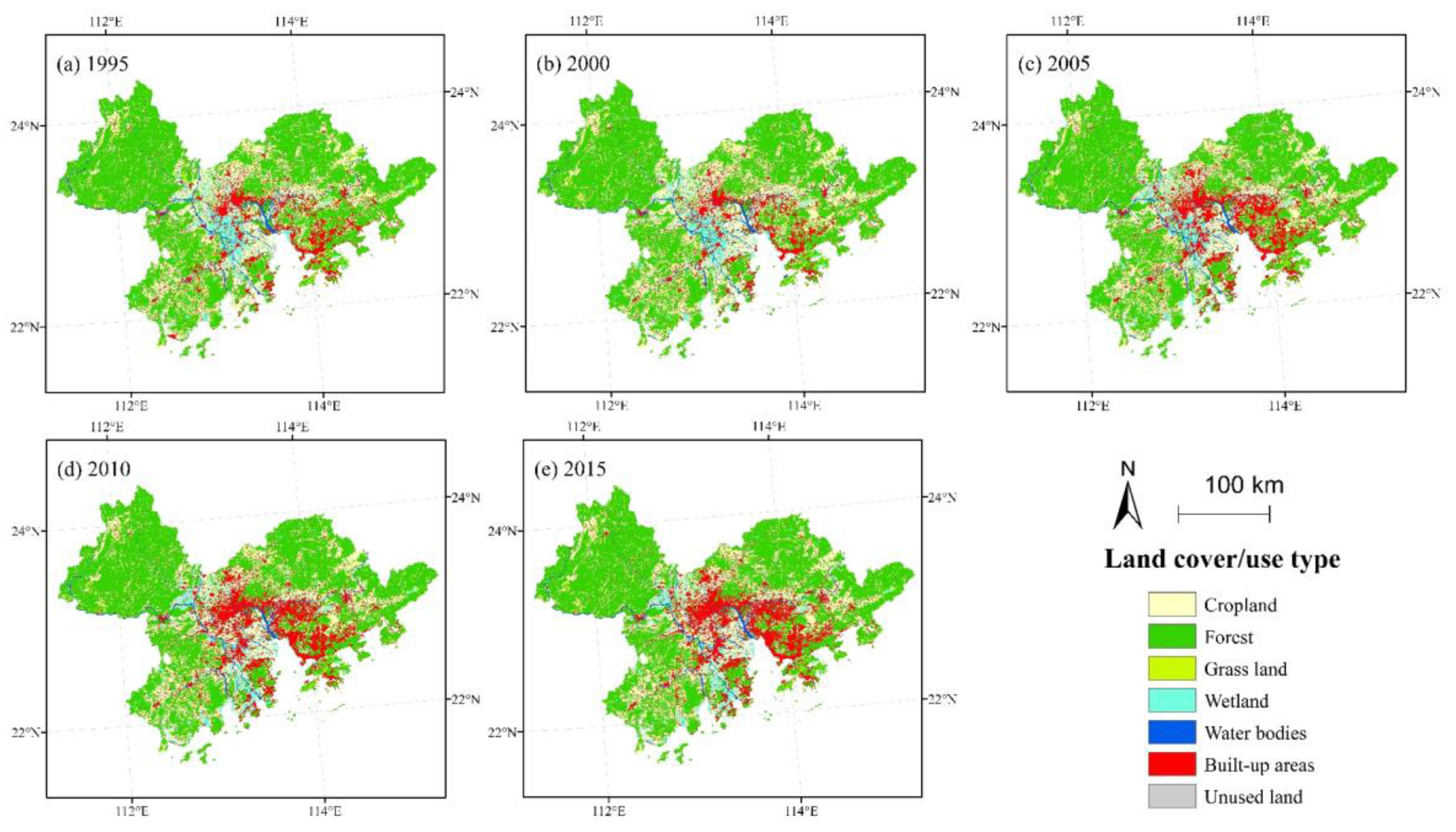
Land use/cover datasets for the years 1995, 2000, 2005, 2010 and 2015 used China land use/cover change (CNLUCC) data provided by the Resources and Environmental Sciences, Chinese Academy of Sciences (RESDC; http://www.resdc.cn, DataID = 184; accessed on 24 July 2020). CNLUCC data based on Landsat series satellite remote sensing images were processed using the supervised classification method to divide land cover/use categories with comprehensive accuracy exceeding 90% and a fine spatial resolution of 30 m [37]. In this study, CNLUCC data were reclassified into seven categories: cropland, forest, grassland, water bodies, wetland, built-up areas and unused land. The land use/cover datasets are shown in Figure 2.
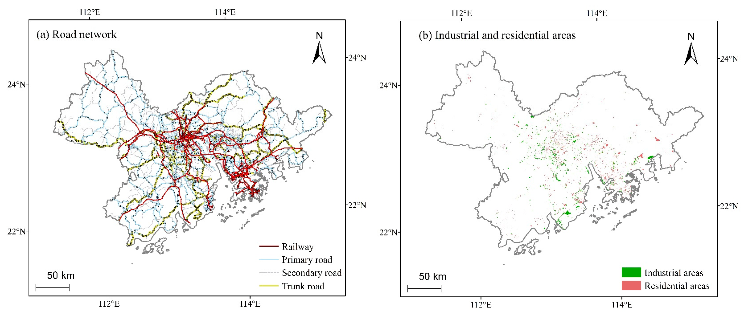
Vector datasets of the road network, residential areas and industrial areas, were obtained from OpenStreetMap (OSM; https://download.geofabrik.de/, accessed on 12 July 2020). We selected road network datasets with railways, primary roads, trunk roads and secondary roads from the attribution of the road layer (fclass) in OSM data. Industry and residential datasets were extracted from the attribution of the land use layer in OSM data. The vector datasets are shown in Figure 3.
Socioeconomic data included population distribution (POP) data and gross domestic product (GDP) data. Population data for the years 2000–2015 were derived from Oak Ridge National Laboratory (ORNL) LandScan global population distribution data at approximately 1 km (30″ × 30″) spatial resolution (https://landscan.ornl.gov/landscan-datasets, accessed on 20 October 2020). This database uses the best available demographic (census) and geographic data and remote sensing imagery techniques within a multivariate asymmetric model to acquire a reliable population distribution data source; the POP data are shown in Figure A1 in Appendix A. POP data in 1995 were obtained from RESDC (http://www.resdc.cn/data.aspx?DATAID=251, accessed on 21 July 2020) with 1 km spatial resolution. The 1 km grid GDP data we used covered the period from 1995 to 2015 and were provided by RESDC (http://www.resdc.cn/data.aspx?DATAID=252, accessed on 22 July 2020). The GDP data are shown in Figure A2.
Impervious surface data were acquired from global artificial impervious area (GAIA) maps (http://data.ess.tsinghua.edu.cn/gaia.html, accessed on 2 November 2020), which provide highly accurate annual GAIA from 1985 to 2018 with 30 m spatial resolution [38]. We extracted the proportion of impervious surface (PIS) using 300 m grids in the years 1995, 2000, 2005, 2010 and 2015, with values ranging from 0 to 1. The PIS is shown in Figure A3.
NDVI datasets were derived at the spatial resolution of 250 m in MOD13Q1 16-day products from LAADS DAAC (https://ladsweb.modaps.eosdis.nasa.gov/, accessed on 15 October 2020), with data from 2000 onwards. We calculated the mean value of NDVI in each year and then estimated fractional vegetation cover (FVC) based on the pixel dichotomy model. NDVI data for 1995 were obtained from the RESDC website (http://www.resdc.cn/DOI/doi.aspx?DOIid=49, accessed on 25 October 2020), which provides NDVI data from 1998 to 2018. We also estimated FVC and conducted correlation analysis using the 1998 NDVI instead of 1995 NDVI. The fractional vegetation cover (FVC) datasets are shown in Figure A4.
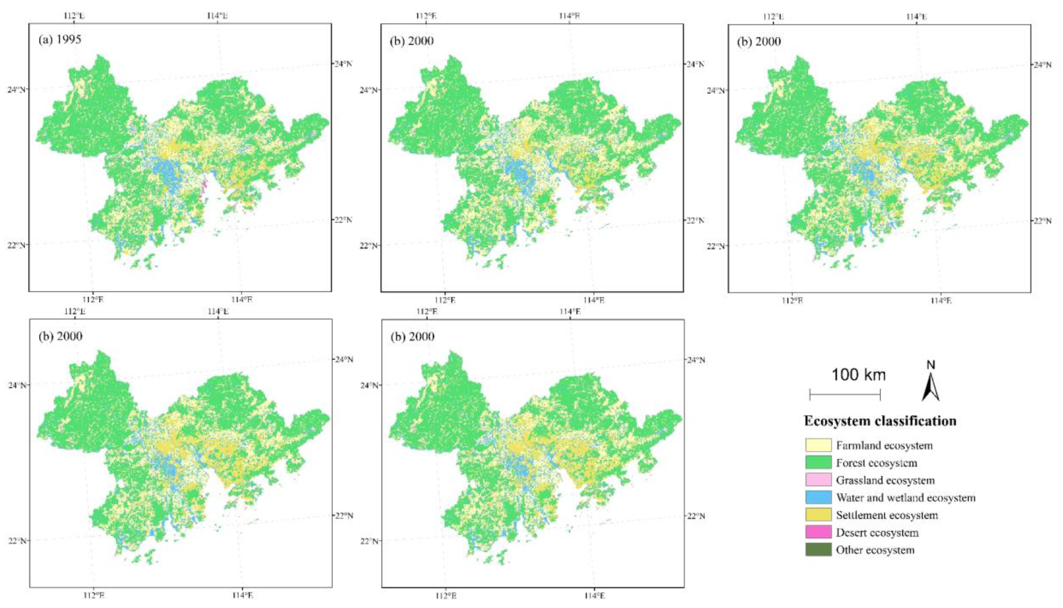
Supplementary analysis datasets in this study included DEM data and terrestrial ecosystem classification data. Terrestrial ecosystem classification data of China were obtained from RESDC (http://www.resdc.cn/data.aspx?DATAID=103, accessed on 28 July 2020) and had seven classifications: farmland, forest, grassland, water and wetland, settlement, desert and other ecosystems. These classification datasets covered the years 1995, 2000, 2005, 2010 and 2015 and were based on 1:100,000 scale land use/cover data. The spatial pattern of the terrestrial ecosystem classification is shown in Figure A5. DEM data at 30 m spatial resolution captured by the Shuttle Radar Topography Mission (SRTM) were downloaded from the Consortium for Spatial Information (CGIAR-CSI; http://srtm.csi.cgiar.org/srtmdata/, accessed on 25 July 2020). The terrestrial ecosystem classification data and DEM data were applied to extract the values of habitat quality, which had been identified using the characteristics of differentiation in habitat quality to extract numerical distribution of habitat quality from different perspectives.
Albers equal-area conic projection was used for all datasets in this study. The central meridian was 105 and the first standard parallel and second standard parallel were 25 and 47, respectively.

2.3. Methods

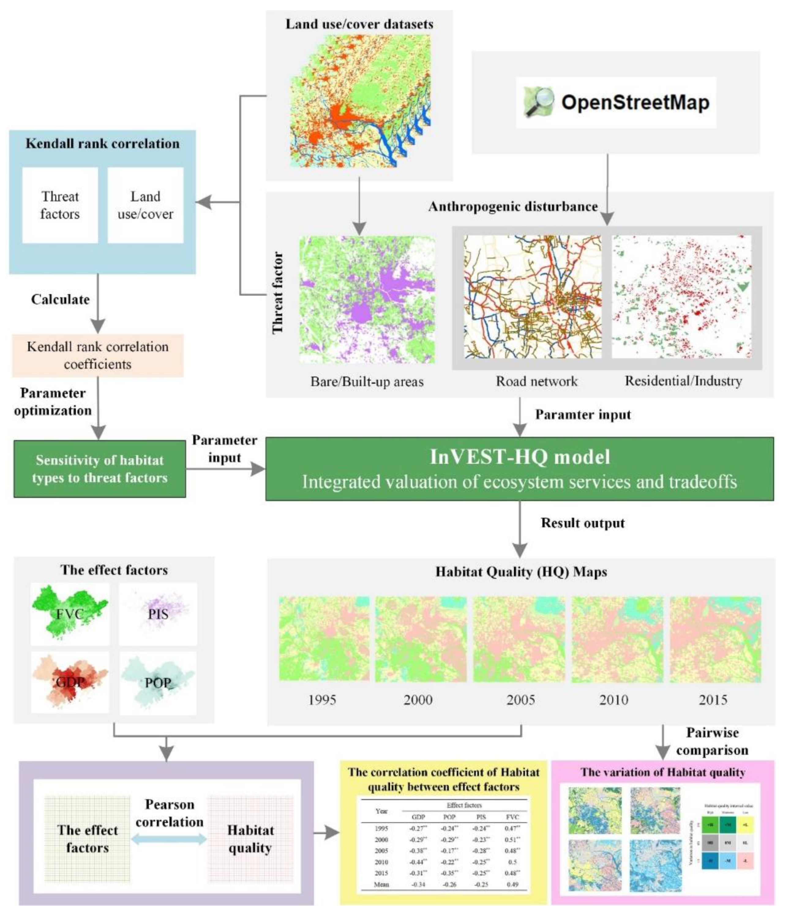
The analysis workflow of this study consisted of four key steps. First, the original parameter of InVEST-HQ—sensitivity of LULC to a threat factor—was calculated by Kendall’s correlation instead of the empirical value. Second, we estimated the habitat quality of the GBA from 1995 to 2015 based on the optimized InVEST-HQ model. Third, we analyzed spatial differentiation in habitat from different perspectives based on different ecosystem classifications and elevational gradients. Fourth, Pearson’s correlations were used to analyze the relationship between the effect factors and habitat quality. The organizational flow chart of this study is shown in Figure 4.

2.3.1. The InVEST Model

The InVEST model is an open-source software model used to visualize and estimate goods and services from nature on a spatial scale; it was developed by Stanford University, Minnesota University, the World Wide Fund and the Nature Conservancy [25]. Habitat quality is one of the modules of the InVEST model which can rapidly estimate the status of habitat for each LULC scale. The InVEST habitat quality (InVEST-HQ) model has been used to assess historic and dynamic changes in habitat quality in Italy [4], China [29,30] and Nicaragua [31]. We used the InVEST-HQ model (InVEST v3.8.7, Stanford University, Stanford, CA, USA) to estimate the habitat quality of the GBA in 1995, 2000, 2005, 2010 and 2015 (model available at https://naturalcapitalproject.stanford.edu/software/invest, accessed on 25 May 2020). More details can be found in the InVEST user’s guide [25] and relevant literature [14,39], while the parameters of the InVEST-HQ model are described here in Section 3.

2.3.2. Kendall’s Rank Correlation Analysis Methods

Kendall’s rank correlation can be applied to measure the strength of dependence between two classified variables. In the InVEST-HQ model, the original parameter in sensitivity of habitat type to threat factor was determined by empirical values for each LULC and threat factor (both variables were categorical datasets which had been classified as 0 or 1). The absolute value of Kendall’s correlation coefficients served as the sensitivity of habitat types to threat factors in the InVEST-HQ model. All correlation coefficients were calculated using R software in this study.
T = | τ | = | n c n d n ( n 1 ) / 2 |
where T is the absolute value of Kendall’s correlation coefficient, τ is Kendall’s correlation coefficient, nc is the number of concordant pairs, nd is the number of discordant pairs, and n is the number of pairs.

2.3.3. Pearson’s Correlation Analysis Methods

Pearson’s correlation analysis was used to investigate the factors affecting habitat quality. Habitat quality is affected by multiple factors. In particular, FVC is an important ecological parameter used for monitoring vegetation cover or forest, POP and GDP are socioeconomic factors that are used to indicate the intensity of human activity, and PIS can indicate the intensity of artificial types of land use. Therefore, POP, PIS, GDP and FVC were selected as the potential effect factors.
The significance of the Pearson’s correlation coefficients were estimated using the t-tests. We calculated the Pearson’s correlation coefficients of all habitat quality datasets and all effect factor datasets from 1995, 2000, 2005, 2010 and 2015.
r = i = 0 N 1 ( x i x ¯ ) ( y i y ¯ ) i = 0 N 1 ( x i x ¯ ) 2 i = 0 N 1 ( y i y ¯ ) 2
where r is the Pearson’s correlation coefficient; xi is the matrix of habitat quality, yi is the matrix of each effect factor, N is the number of matrix elements (x, y both have the same matrix element), and x ¯ ,   y ¯ are the mean values of habitat quality and effect factor, respectively.

2.3.4. Variation in Habitat Quality Analysis

A series of habitat quality maps were acquired using the InVEST-HQ model in different years, with the habitat quality scoring between 0 and 1 in each cell. To ascertain the spatiotemporal variation in habitat quality, we referred to the categorized method of Czekajlo et al. [40] on greenness score, which had a similar application environment. This method could express variation at different levels and incorporate the current state with historic trends [40].
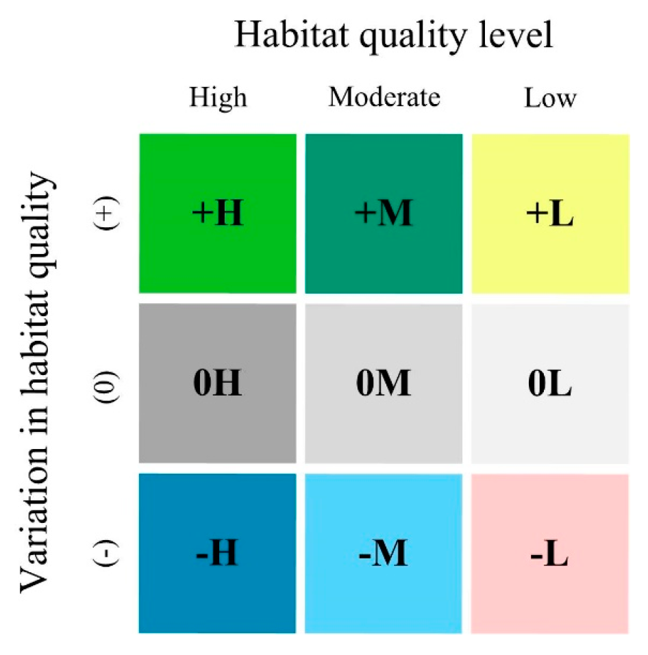
In this study, we calculated four comparison groups for a pair-wise comparison sequence between 1995 and 2000, 2000 and 2005, 2005 and 2010, and 2010 and 2015. The difference maps were divided into three classes (decrease (−): difference value less than 0; not significant (0): difference value equal to 0; and increase (+): difference value greater than 0). Then, the habitat quality score (0–1) was categorized into three levels using natural breaks (Jenks) in each year, namely, low (L), moderate (M) and high (H). Last, we acquired 9 variation categories in each difference value group, with each difference value class marked by three habitat quality score levels. The habitat quality variation in this study was categorized by the last year of the comparison (e.g., when comparing a pair-wise sequence between 1995 and 2000, the habitat quality score in 2000 was selected as the categorized level). Natural breaks (Jenks) is an unsupervised classification, which was also successfully applied in another study [40,41]. The categories of variation in habitat quality are shown in Figure 5.

3. Model Parameter Settings

The parameters of the InVEST-HQ model in this study include LULC maps, a raster layer of threat factors, the weight of each threat factor, the maximum distance of each threat factor, the sensitivity score of habitat types to threat factors, and the habitat suitability score. The data resources and descriptions are given in Table 2. The details of the parameter settings will be given in the following sections.

3.1. Threat Factor Parameters

Defining the threat factor parameter for a habitat is a key issue in the InVEST-HQ model [27]. Threat factors include biotic factors (e.g., alien species invasion), abiotic factors (e.g., sunshine duration, temperature, precipitation) and anthropogenic disturbance (e.g., land use change, roads, rural settlements) [30]. Anthropogenic disturbance has been considered in relation to ecology and the environment in previous studies, which have focused on the impact of land use change [30,42,43], and the threat of land use change and roads [31]. In this study, we selected threat factors from anthropogenic disturbance based on the study of Sallustio et al. [4] and the actual situation of the GBA.
The GBA has experienced rapid development and change in land use/cover due to accelerated industrialization and urbanization [44]. Artificial land use/cover types (e.g., cropland, urban areas, plantations) have expanded, undermining ecosystem services along with considerable losses of biodiversity [45]. Artificial land use/cover types should be considered as threat factors, as the most direct manifestation of anthropogenic disturbance to the ecosystem [30]. The transport network has a cumulative and irreversible effect on ecosystem services and biodiversity, and its construction has resulted in habitat fragmentation and has become a severe threat [46,47,48]. We selected cropland, built-up areas and bare land from the LULC map, and road networks (including railways, primary roads, trunk roads and secondary roads), residential and industrial areas from OSM data as they are consistent with these threat factors.
The parameter of threat factors included weight, maximum distance and decay type, which were determined by empirical values or expert knowledge. We determined the weight, maximum distance, and decay type of each threat factor based on relevant studies [4,27,30,31] carried out in similar circumstances, the actual situation of the GBA, and the InVEST model user’s guide [25]. The threat factor parameters of this study are listed in Table 3.
The near edge of the threat factor should be considered which will influence the habitat quality result in the InVEST-HQ model [25]. In this study, we defined the buffer width of road networks, industry and residential activity, then we converted the vector buffer file into a raster surface. The buffer widths were based on Aneseyee et al. [49]: 1.5 km for trunk road, 1.5 km for railway, 1 km for primary road, 0.5 km for secondary road, 0.5 km for residential areas and 1 km for industrial areas. All maps consisted of a value of 1 or 0, where 1 indicated the presence of a threat and 0 indicated the absence of threat.

3.2. Habitat Suitability Score

In the InVEST-HQ model, the habitat suitability score is a numerical parameter based on LULC types regarded as suitable habitat. Each LULC type gives a habitat suitability score with a value ranging from 0 to 1, where a value of 1 indicates the most suitable habitat. We assumed each LULC type was suitable according to the habitat suitability score in the InVEST user’s guide [25] with a consideration for overall biodiversity (γ biodiversity) in the GBA. Built-up areas and unused land that were not suitable habitat were set at a value of 0, while forest and wetland were set the value 1; other LULC values were based on relevant literature [4,27] and the InVEST user’s guide [25]. The habitat suitability scores are shown in Table 4.

3.3. Sensitivity of Habitat Types to Threat Factors

The sensitivity of habitat types to threat factors was a numerical parameter given for each LULC type between each threat factor in the InVEST-HQ model, with the value ranging from 0 to 1, with 1 representing high sensitivity to a threat factor. The original parameter of the sensitivity score for LULC to the threat factor within the model were based on the empirical value [50], which generally relies on expert knowledge, meaning that the InVEST-HQ model is implicitly subjective and limited in terms of applicability to special regions.
Therefore, finding an approach which could acquire objective regional representative parameters was deemed necessary. We used Kendall’s correlation analysis to calculate the correlation coefficients between each LULC type and each threat factor in different years, in an attempt to address the limitations of the sensitivity score in the InVEST-HQ model. The method was described in Section 2.3.2 and the results are shown in Table A1.

4. Results and Analyses

4.1. Characteristic of Spatiotemporal Pattern in Habitat Quality

4.1.1. Spatial Pattern of Habitat Quality

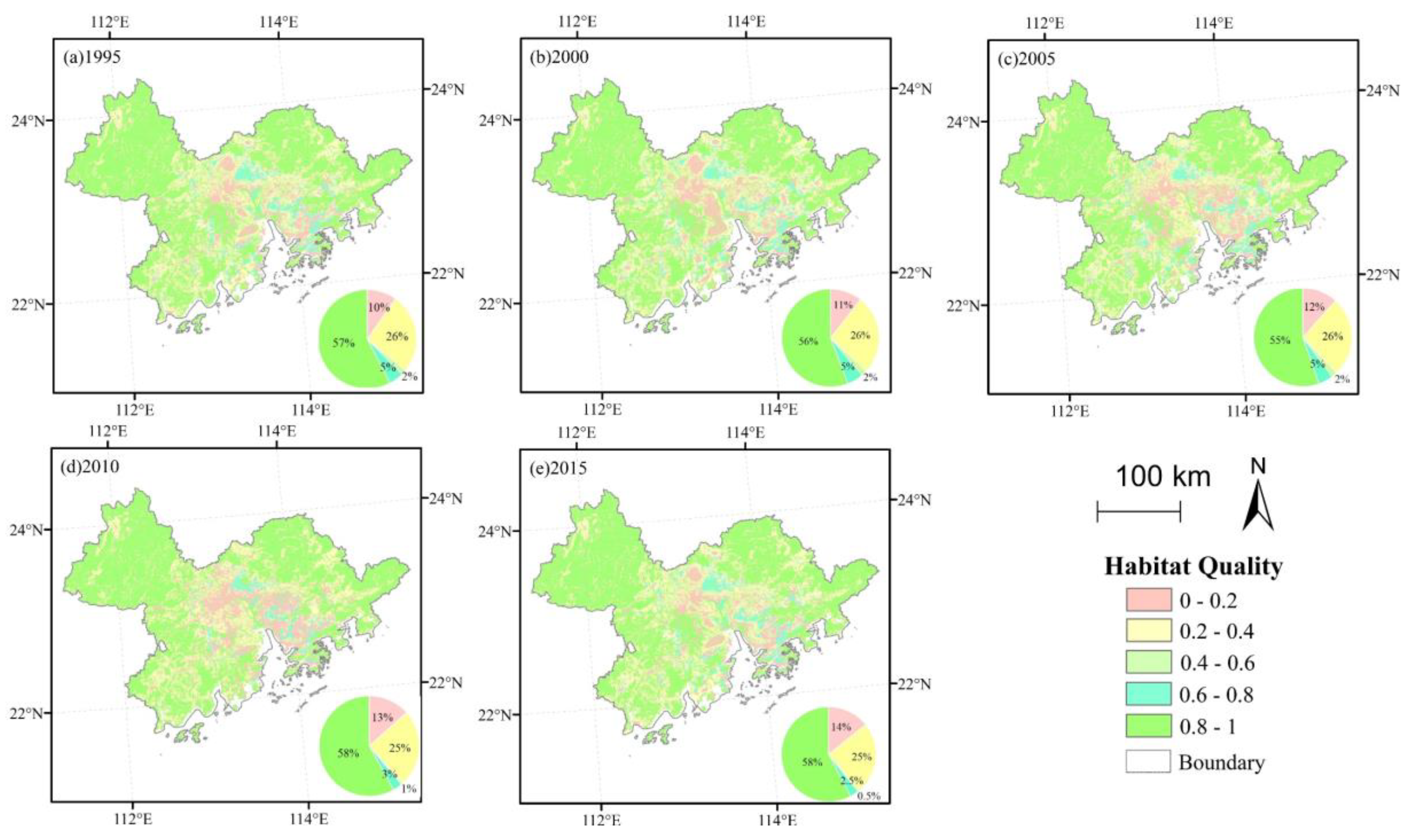
Figure 6 shows the spatial pattern of habitat quality in the GBA with a range of habitat quality values between 0 and 1 (higher values indicating a more suitable habitat). The spatial pattern displays that the habitat quality index increased from the center to the fringe areas in the period from 1995 to 2015, with some small differences in central areas between years. The overall level of habitat quality was high over the entire study period, with an average score of 0.61, 0.60, 0.59, 0.60 and 0.60 in 1995, 2000, 2005, 2010 and 2015, respectively. The dominant level of high habitat quality (0.8–1) was greater than or equal to 55% and was mainly distributed in the outer ring of the GBA, especially in Zhaoqing, Jiangmen and Huizhou. These areas were dominated by forest in mountain areas with high vegetation fraction cover. The land use intensity was relatively low and the vegetation cover was dense [51], suggesting that the biodiversity value in fringe areas was significantly higher than in central areas. The next most highly distributed levels of habitat quality were the mid-low level (0.2–0.4) and the low level (0–0.2), which accounted for 25% and 10%, respectively, and were concentrated in the central areas of the GBA such as Guangzhou, Shenzhen and Foshan. These areas were dominated by serried industry parks and built-up land with a high intensity of human activities, and thus do not provide much suitable habitat for wildlife. The medium habitat quality level was less than or equal to 5% with a dispersed distribution in Hong Kong, Guangzhou and Dongguan, while the mid-high level had a low distribution of less than or equal to 5% of the total area.

4.1.2. Spatial Pattern of Habitat Quality from Different Perspectives

To evaluate the characteristics of spatial patterns from different ecosystem perspectives, we used the terrestrial ecosystem classification data to extract habitat quality values over the period from 1995 to 2015. As shown in Figure 7, different ecosystem classifications showed a discrepancy in the distribution of habitat quality scores. Farmland and settlements had a consistent distribution with a large value range over the period from 1995 to 2015, which indicates that habitat quality differed within the same ecosystem classification, which could be attributed to differences in climate and elevation. The forest ecosystem had the highest value of habitat quality and was overall close to 1 during the period from 1995 to 2015, which indicates that the forest ecosystem provides a suitable habitat and has high biodiversity value. The grassland ecosystem showed a stable distribution of habitat quality value. Other ecosystems had consistent distributions during the studied period, except for 1995. The desert ecosystem was eliminated from this study because the sample size of this ecosystem was too small to analyze.
To understand the characteristics of spatial patterns from the elevational perspective, a DEM was used to extract habitat quality values at different elevational gradients over the period 1995–2015 (Figure 8). Overall, the habitat quality has an increasing trend with elevation. There was a cluster of habitat quality values in the range of 0.25 to 0.4, which does not change with elevation in the region. It was indicated that this range of habitat quality (0.25 to 0.4) was majorly distributed in plain areas. However, there is a significant trend in the range of 0.5 to 1 that showed that habitat quality increased with altitude, indicating that high habitat quality may be related to elevation. A study in Nanshi Lake basin verified that elevation was significantly correlated with habitat quality [30]. However, this finding differs from a study in the Omo-Gibe Basin, as a different pattern of altitude to habitat quality showed a decreasing trend in the Winike watershed [49].

4.2. Characteristics of Spatiotemporal Variation in Habitat Quality

Spatiotemporal Variation of Habitat Quality

The spatiotemporal variation in habitat quality is shown in Figure 9. In general, the variation in habitat quality in the GBA revealed a conspicuous change in the study years that tended toward habitat degradation overall, except for the period from 1995 to 2000. In the interval value of habitat quality level (low (L), moderate (M) and high (H)) perspective, the high level of habitat quality (e.g., (+H) and (−H)) had a dramatic change with a large distribution in the entire studied period. The moderate level had a small distribution in Guangzhou for the period of 1995 to 2010, though a comparatively larger distribution than that for Foshan, Zhongshan and Dongguan during the period from 2010 to 2015. From the variation perspective, the changing levels of habitat quality showed significant spatial differentiation. The areas with no change (0) were mainly distributed in the cities of central GBA, such as Dongguan, Foshan, Guangzhou and Shenzhen, and had a gradual expansion throughout the course of the studied period. The changing areas in the period from 1995 to 2000 showed that habitat quality improved, with overall positive variation and little habitat degradation in Shenzhen, Foshan and Hong Kong. The variation in the period from 2000 to 2005 showed both positive and negative patterns. However, there was a general decrease both in the period from 2005 to 2010 and from 2010 to 2015.

4.3. Analysis of the Variation of Habitat Quality and Effect Factor

In the period from 1995 to 2000 the habitat quality improved; however, habitat degradation was the general pattern for the GBA during the period from 2000 to 2015. This was associated with multiple factors, such as human activities, land use change and vegetation loss. The effect of land use change was reflected by built-up area expansion and forest land fragmentation. The built-up area increased rapidly from 8.77% to 14.18%, and the area of forest land decreased from 56.42% to 53.94% in the GBA during the period from 1995 to 2015. However, in the period from 1995 to 2000, the percentage of built-up land slightly declined, as shown in Figure 10.
Human activities and vegetation loss were important factors affecting habitat quality in the GBA and, based on the Pearson’s correlation coefficient relating habitat quality to each effect factor in different years, they showed a significant correlation (Table 5; except for FVC in 2010). FVC, which represented natural vegetation cover, had a strong positive linear relationship with habitat quality. This result indicated that vegetation loss led to habitat degradation. Vegetation loss in urban agglomerations especially decreased the capacity of the urban ecosystem to provide obligatory ecosystem services [49]. POP, PIS and GDP were used to embody human activities, and they had a significant negative linear correlation with habitat quality, which revealed that natural habitat degradation was a result of the growth in population, economic development and the expansion of impervious surface cover. Human activities were verified here as the largest threats to the ecological environment and biodiversity in the GBA. Our findings are similar to those of a previous study of ecological quality in the GBA, which reported that urban expansion and policy variation had a dominant influence on habitat change [52], and another study on the habitat quality of the Pearl River delta found that habitat quality was significantly affected by population and economic density [51].

5. Discussion

5.1. The Role of Sensitivity of Habitat Type to Threat Factors in the InVEST Habitat Quality Model

The sensitivity of habitat types to threat factors is a parameter that uses a value from 0 to 1 to indicate the degree to which the habitat type is affected by each threat factor [25]. A sensitivity value close to 1 signifies that the habitat type is heavily degraded by the threat factor. As mentioned in Section 3.3, the original sensitivity scores were set by an empirical value and relied on an expert knowledge system [25]. However, this parameter is difficult to acquire in some study areas, and gives the HQ model a subjective tendency. Therefore, finding a way to determine sensitivity of habitat types to threat factors using the InVEST-HQ model was considered important in this study. Kendall’s correlation coefficient can describe the strength of association between two categorical variables [53] and has been successfully used in other fields [54,55]. For the InVEST-HQ model we used, the sensitivity of each habitat type to threat factors was estimated by the Kendall’s correlation coefficient (LULC datasets and threat factors were both categorical data), which could calculate an objective sensitivity value specific to the GBA. A limitation of this study is that the results of this strategy to calculate sensitivity were not compared with other strategies, such as the expert-based strategy.

5.2. Exploring the Use of Assessment of Habitat Quality for Biodiversity Conservation

The InVEST-HQ model evaluates habitat quality as an ecological indicator at the landscape scale which can be a proxy for regional biodiversity [27,28]. The model depends on the accessibility and intensity of artificial land use/cover types [56,57]. Recently, the InVEST-HQ model was used to assess the status of biodiversity and habitats worldwide, which could reveal spatial and temporal changes of biodiversity at the largest scale [58].
In this study, the results of the InVEST-HQ model will help to understand the spatial distribution of habitat quality with a consideration for general biodiversity. We obtained a series of habitat quality maps for different years. There was a characteristic spatial pattern which showed increased habitat quality from the center to fringe areas and showed a significant difference among ecosystem classifications and an increase of habitat quality with elevation. This finding can be applied to understand the biodiversity status of the GBA, which could help evaluate the strategies for biodiversity conservation in the region and assist in prioritizing habitat conservation units. A similar mechanism of spatial distribution of habitat quality was observed in other areas, e.g., Nansihu lake basin, China [30], Changli county, China [59], and Italy [4].
The spatiotemporal variation of habitat quality was affected by multiple factors in this study, such as human activities, land use change and vegetation loss. Vegetation loss and intense human activity were the most important factors of habitat degradation, with built-up area expansion and forest land fragmentation as the most clear expressions of land use change. It is necessary in studies of the urban ecosystem to explore the tradeoff areas between nature conservation and economic development, especially in the GBA. Many studies have focused on habitat quality and its influencing factors, such as a study of the habitat quality in Yangtze River Delta Regional, China, which found a significant negative relationship with urbanization intensity [60], and a study of protected areas in Italy found that increased human population density led to a decreasing trend in habitat quality [4].

5.3. Limitations and Future Outlook

The InVEST-HQ model is flexible in terms of parameter settings, which facilitated the integration of a different concept for habitat threat data and its attributes. In particular, the threat factor could be divided into three types: biotic factors, abiotic factors and anthropogenic disturbances [30]. We focused on anthropogenic threats in the InVEST-HQ model in this study. To express the impact of anthropogenic disturbance on habitat quality, we selected cropland, built-up area, bare land, the road network, and residential and industrial areas. However, it is worth noting that we assumed all native species and habitats in the study area were impacted by these threat factors, and we ignored possible alternative consequences. This assumption in relation to threat factors was similar with previous studies, such as a study in Nansihu lake basin, China [30], a study in the state of Minnesota, USA [61], a study in Chaharmahal and Bakhtiari province, Iran [47], and a study in the areas of Hohhot-Baotou-Ordos-Yulin, China [32]. We recognize that this approach could be improved by selecting more threat factors in future studies.
We used Kendall’s correlation analysis to acquire a series of objective sensitivity scores for habitat types to threat factors. Although this study attempted to improve the objectivity by the correlation analysis method, there were some limitations for the other parameters. The weight of the threat factors, the maximum distance of threat factors, and habitat suitability scores were determined by empirical values and expert knowledge, which resulted in some inevitable subjectivity. Previous studies have also optimized some parameters; for example, a study obtained habitat suitability scores by integrating a soil degradation index with the aboveground habitat condition [62], another study obtained habitat suitability scores based on a species distribution model and expert opinion [63], future land use cover types were obtained in a study by cellular automata in different future scenarios, which could predict the future variation in habitat quality [42]. In a future study, we should attempt to find more approaches to add objectivity to the InVEST-HQ model.
Our results of habitat quality in different years were not compared with field site data. The unverified calibration of the field investigation may lead to some uncertainty in the results of the InVEST-HQ model. To overcome this limitation, future studies should obtain a comparison of the performance of our model with other ecological process models, or carry out a field investigation of habitat to calibrate the InVEST-HQ model.

6. Conclusions

In this study we used the Kendall’s correlation coefficient of land use/cover types and threat factors instead of the sensitivity of habitat types to threat factor parameter provided in the InVEST-HQ model. Then, we estimated the spatiotemporal pattern and variation in habitat quality in the GBA during the period from 1995 to 2015 based on the optimized InVEST-HQ model. We analyzed the differentiation of habitat quality across different ecosystem classifications and elevation gradients. Finally, we analyzed the relationship between habitat quality, vegetation cover and anthropogenic threats using Pearson’s correlation coefficients.
Our results indicated that the spatial pattern of habitat quality decreased from fringe areas to central areas, showing significant differences for different ecosystem classifications and elevational gradients. In the period from 1995 to 2015, habitat quality declined as a result of vegetation loss, land use change and intense human activity, and the fraction of vegetation cover was an important effect factor of habitat quality, with a strong positive linear relationship. Human activities were the largest threat to the ecological environment in the GBA, with a significant negative linear relationship. The expansion of built-up areas and forest land fragmentation were clear expressions of land use change. Our method provides an operational approach to evaluating the availability of management strategies for biodiversity conservation and a unique perspective of sustainable development in urban agglomerations that could be used to explore tradeoffs between natural habitats and economic development. The unverified calibration of the field investigation might lead to some uncertainty in the results. Future studies should focus on a comparison of the performance of other ecological process models or design an investigation of habitat to overcome this limitation.
We attempted to develop an optimization method to improve the objectivity of the InVEST-HQ model, and to calculate the sensitivity of habitat types to threat factors by Kendall’s correlation coefficient, which provided an objective and applicable sensitivity value for the GBA. However, a comparison was not made with the original strategy, so future studies should address this limitation.

Author Contributions

Conceptualization, L.W., C.S., and F.F.; Supervision, C.S., and F.F.; Writing—original draft, L.W.; Writing—review and editing, C.S., and F.F. All authors have read and agreed to the published version of the manuscript.

Funding

This research was funded by the National Nature Science Foundation of China (Grant No. 41901347), Guangdong Basic and Applied Basic Research Foundation (Grant No. 2020A1515010562) and the China Postdoctoral Science Foundation (Grant No. 2018M643109).

Acknowledgments

We sincerely thank the reviewers for their helpful comments and suggestions about our manuscript.

Conflicts of Interest

The authors declare no conflict of interest.

Appendix A

Figure A1 and Figure A2 show the population distribution and gross domestic product distribution in the years 1995, 2000, 2005, 2010 and 2015.
Figure A1. The spatial distribution of population: (a) 1995, (b) 2000, (c) 2005, (d) 2010, (e) 2015.
Remotesensing 13 01008 g0a1
Figure A2. The spatial distribution of gross domestic product: (a) 1995, (b) 2000, (c) 2005, (d) 2010, (e) 2015.
Remotesensing 13 01008 g0a2
Figure A3. The spatial pattern of the proportion of impervious surfaces: (a) 1995, (b) 2000, (c) 2005, (d) 2010, (e) 2015.
Remotesensing 13 01008 g0a3
Figure A4. The spatial pattern of fractional vegetation cover in (a) 1995, (b) 2000, (c) 2005, (d) 2010, and (e) 2015.
Remotesensing 13 01008 g0a4
The terrestrial ecosystem classification data was obtained from RESDC and is shown in Figure A5. These data were classified into farmland, forest, grassland, water and wetland, settlement, desert, and other ecosystems.
Figure A5. The spatial pattern of terrestrial ecosystem classification in (a) 1995, (b) 2000, (c) 2005, (d) 2010, and (e) 2015.
Remotesensing 13 01008 g0a5
Table A1 shows the absolute value of Kendall’s correlation coefficient for each LULC type and threat factor, which were used to replace the original parameter of the InVEST-HQ model.
Table A1. The sensitivity score of habitat types to threat factors.
YearLULC TypesThreat Factors
CroplandBuilt-Up AreasBare LandRail-WayTrunk RoadPrimary RoadSecondary RoadIndustry ActivityResidential
1995Cropland10.170.010.040.080.10.080.040.04
Forest0.60.330.010.20.220.240.240.220.19
Grass land0.090.0500.010.020.010.030.010.01
Wetland0.130.0700.050.080.060.060.120.03
Water bodies0.080.0500.020.040.030.020.070.01
Built-up areas0.17100.250.240.260.290.190.27
Unused land0.010.010.350.0100.0100.020
2000Cropland10.170.030.050.080.110.090.040.05
Forest0.620.310.050.190.220.240.240.220.19
Grass land0.090.040.30.010.010.020.020.020.01
Wetland0.140.070.010.040.070.050.060.110.02
Water bodies0.090.040.010.020.040.020.010.060
Built-up areas0.1710.010.240.240.250.280.190.27
Unused land0.010.010.210.010.01000.010.01
2005Cropland10.14000.050.080.040.020.02
Forest0.580.370.010.20.230.250.250.230.19
Grass land0.080.0500.010.010.020.030.020.01
Wetland0.130.0800.030.050.030.040.090.01
Water bodies0.080.0500.020.040.020.010.060
Built-up areas0.15100.240.240.250.280.190.24
Unused land0.010.010.770.010000.010.01
2010Cropland10.2000.050.080.040.020.02
Forest0.560.40.010.210.230.250.250.230.2
Grass land0.070.0500.010.020.020.030.020.01
Wetland0.120.0900.010.01000.020.02
Water bodies0.080.0600.020.040.030.010.060.01
Built-up areas0.2100.30.280.30.350.280.29
Unused land0.010.010.690.010000.010
2015Cropland10.2100.010.050.070.030.070.02
Forest0.550.410.010.210.230.250.250.230.2
Grass land0.080.0600.020.020.030.030.020.02
Wetland0.120.0900.010.01000.020.02
Water bodies0.080.0600.020.040.030.010.060.01
Built-up areas0.21100.310.290.30.360.290.29
Unused land0.010.010.720.0100000

References

  1. Baeten, L.; Hermy, M.; Van Daele, S.; Verheyen, K. Unexpected understorey community development after 30 years in ancient and post-agricultural forests. J. Ecol. 2010, 98, 1447–1453. [Google Scholar] [CrossRef] [Green Version]
  2. Daskalova, G.N.; Myers-Smith, I.H.; Bjorkman, A.D.; Blowes, S.A.; Supp, S.R.; Magurran, A.E.; Dornelas, M. Landscape-scale forest loss as a catalyst of population and biodiversity change. Science 2020, 368, 1341–1347. [Google Scholar] [CrossRef]
  3. Newbold, T.; Hudson, L.N.; Hill, S.L.L.; Contu, S.; Lysenko, I.; Senior, R.A.; Börger, L.; Bennett, D.J.; Choimes, A.; Collen, B.; et al. Global effects of land use on local terrestrial biodiversity. Nat. Cell Biol. 2015, 520, 45–50. [Google Scholar] [CrossRef] [Green Version]
  4. Sallustio, L.; De Toni, A.; Strollo, A.; Di Febbraro, M.; Gissi, E.; Casella, L.; Geneletti, D.; Munafò, M.; Vizzarri, M.; Marchetti, M. Assessing habitat quality in relation to the spatial distribution of protected areas in Italy. J. Environ. Manag. 2017, 201, 129–137. [Google Scholar] [CrossRef]
  5. Ng, C.N.; Xie, Y.J.; Yu, X.J. Measuring the spatio-temporal variation of habitat isolation due to rapid urbanization: A case study of the Shenzhen River cross-boundary catchment, China. Landsc. Urban Plan. 2011, 103, 44–54. [Google Scholar] [CrossRef]
  6. Wilson, M.C.; Chen, X.-Y.; Corlett, R.T.; Didham, R.K.; Ding, P.; Holt, R.D.; Holyoak, M.; Hu, G.; Hughes, A.C.; Jiang, L.; et al. Erratum to: Habitat fragmentation and biodiversity conservation: Key findings and future challenges. Landsc. Ecol. 2015, 31, 229–230. [Google Scholar] [CrossRef] [Green Version]
  7. Bongaarts, J. IPBES, Summary for policymakers of the global assessment report on biodiversity and ecosystem services of the Intergov-ernmental Science-Policy Platform on Biodiversity and Ecosystem Services. Popul. Dev. Rev. 2019, 45, 680–681. [Google Scholar] [CrossRef] [Green Version]
  8. Oliver, T.H.; Heard, M.S.; Isaac, N.J.; Roy, D.B.; Procter, D.; Eigenbrod, F.; Freckleton, R.; Hector, A.; Orme, C.D.L.; Petchey, O.L.; et al. Biodiversity and Resilience of Ecosystem Functions. Trends Ecol. Evol. 2015, 30, 673–684. [Google Scholar] [CrossRef] [Green Version]
  9. Vellend, M.; Baeten, L.; Myers-Smith, I.H.; Elmendorf, S.C.; Beauséjour, R.; Brown, C.D.; De Frenne, P.; Verheyen, K.; Wipf, S. Global meta-analysis reveals no net change in local-scale plant biodiversity over time. Proc. Natl. Acad. Sci. USA 2013, 110, 19456–19459. [Google Scholar] [CrossRef] [PubMed] [Green Version]
  10. Dornelas, M.; Gotelli, N.J.; McGill, B.; Shimadzu, H.; Moyes, F.; Sievers, C.; Magurran, A.E. Assemblage Time Series Reveal Biodiversity Change but Not Systematic Loss. Science 2014, 344, 296–299. [Google Scholar] [CrossRef] [Green Version]
  11. Magurran, A.E.; Deacon, A.E.; Moyes, F.; Shimadzu, H.; Dornelas, M.; Phillip, D.A.T.; Ramnarine, I.W. Divergent biodiversity change within ecosystems. Proc. Natl. Acad. Sci. USA 2018, 115, 1843–1847. [Google Scholar] [CrossRef] [Green Version]
  12. Yoccoz, N.G.; Ellingsen, K.E.; Tveraa, T. Biodiversity may wax or wane depending on metrics or taxa. Proc. Natl. Acad. Sci. USA 2018, 115, 1681–1683. [Google Scholar] [CrossRef] [Green Version]
  13. Hall, L.S.; Krausman, P.R.; Morrison, M.L. The Habitat Concept and a Plea for Standard Terminology. Wildl. Soc. Bull. 1997, 25, 173–182. [Google Scholar]
  14. Terrado, M.; Sabater, S.; Chaplin-Kramer, B.; Mandle, L.; Ziv, G.; Acuña, V. Model development for the assessment of terrestrial and aquatic habitat quality in conservation planning. Sci. Total. Environ. 2016, 540, 63–70. [Google Scholar] [CrossRef] [Green Version]
  15. Thomas, J.A.; Bourn, N.A.D.; Clarke, R.T.; Stewart, K.E.; Simcox, D.J.; Pearman, G.S.; Curtis, R.; Goodger, B. The quality and isolation of habitat patches both determine where butterflies persist in fragmented landscapes. Proc. R. Soc. Lond. Ser. B Biol. Sci. 2001, 268, 1791–1796. [Google Scholar] [CrossRef]
  16. Fahrig, L. Effects of Habitat Fragmentation on Biodiversity. Annu. Rev. Ecol. Evol. Syst. 2003, 34, 487–515. [Google Scholar] [CrossRef] [Green Version]
  17. Howell, C.A.; Latta, S.C.; Donovan, T.M.; Porneluzi, P.A.; Parks, G.R.; Faaborg, J. Landscape effects mediate breeding bird abundance in midwestern forests. Landsc. Ecol. 2000, 15, 547–562. [Google Scholar] [CrossRef]
  18. Johnson, M.D. Measuring Habitat Quality: A Review. Condor 2007, 109, 489–504. [Google Scholar] [CrossRef]
  19. Sutherland, W.J. The effect of local change in habitat quality on populations of migratory species. J. Appl. Ecol. 1998, 35, 418–421. [Google Scholar] [CrossRef]
  20. Miller, J.R.; Groom, M.; Hess, G.R.; Steelman, T.; Stokes, D.L.; Thompson, J.; Bowman, T.; Fricke, L.; King, B.; Marquardt, R. Biodiversity Conservation in Local Planning. Conserv. Biol. 2009, 23, 53–63. [Google Scholar] [CrossRef] [PubMed]
  21. Beumer, L.T.; Van Beest, F.M.; Stelvig, M.; Schmidt, N.M. Spatiotemporal dynamics in habitat suitability of a large Arctic herbivore: Environmental heterogeneity is key to a sedentary lifestyle. Glob. Ecol. Conserv. 2019, 18, e00647. [Google Scholar] [CrossRef]
  22. Srivastava, V.; Griess, V.C.; Padalia, H. Mapping invasion potential using ensemble modelling. A case study on Yushania maling in the Darjeeling Himalayas. Ecol. Model. 2018, 385, 35–44. [Google Scholar] [CrossRef]
  23. Elith, J.; Leathwick, J.R. Species Distribution Models: Ecological Explanation and Prediction Across Space and Time. Annu. Rev. Ecol. Evol. Syst. 2009, 40, 677–697. [Google Scholar] [CrossRef]
  24. Mocq, J.; St-Hilaire, A.; Cunjak, R. Assessment of Atlantic salmon (Salmo salar) habitat quality and its uncertainty using a multiple-expert fuzzy model applied to the Romaine River (Canada). Ecol. Model. 2013, 265, 14–25. [Google Scholar] [CrossRef]
  25. Sharp, R.; Douglass, J.; Wolny, S.; Arkema, K.; Bernhardt, J.; Bierbower, W.; Chaumont, N.; Denu, D.; Fisher, D.; Glowinski, K.; et al. InVEST 3.8.7. User’s Guide; Collaborative publication by The Natural Capital Project, Stanford University, University of Minnesota, The Nature Conservancy, and World Wildlife Fund; Stanford University: Stanford, CA, USA, 2020. [Google Scholar]
  26. Alkemade, R.; Van Oorschot, M.; Miles, L.; Nellemann, C.; Bakkenes, M.; Brink, B.T. GLOBIO3: A Framework to Investigate Options for Reducing Global Terrestrial Biodiversity Loss. Ecosystems 2009, 12, 374–390. [Google Scholar] [CrossRef] [Green Version]
  27. Zhu, C.; Zhang, X.; Zhou, M.; He, S.; Gan, M.; Yang, L.; Wang, K. Impacts of urbanization and landscape pattern on habitat quality using OLS and GWR models in Hangzhou, China. Ecol. Indic. 2020, 117, 106654. [Google Scholar] [CrossRef]
  28. Chiang, L.-C.; Lin, Y.-P.; Huang, T.; Schmeller, D.S.; Verburg, P.H.; Liu, Y.-L.; Ding, T.-S. Simulation of ecosystem service responses to multiple disturbances from an earthquake and several typhoons. Landsc. Urban Plan. 2014, 122, 41–55. [Google Scholar] [CrossRef]
  29. Xu, L.; Chen, S.S.; Xu, Y.; Li, G.; Su, W. Impacts of Land-Use Change on Habitat Quality during 1985–2015 in the Taihu Lake Basin. Sustainability 2019, 11, 3513. [Google Scholar] [CrossRef] [Green Version]
  30. Sun, X.; Jiang, Z.; Liu, F.; Zhang, D. Monitoring spatio-temporal dynamics of habitat quality in Nansihu Lake basin, eastern China, from 1980 to 2015. Ecol. Indic. 2019, 102, 716–723. [Google Scholar] [CrossRef]
  31. Hack, J.; Molewijk, D.; Beißler, M.R. A Conceptual Approach to Modeling the Geospatial Impact of Typical Urban Threats on the Habitat Quality of River Corridors. Remote Sens. 2020, 12, 1345. [Google Scholar] [CrossRef] [Green Version]
  32. Song, S.; Liu, Z.; He, C.; Lu, W. Evaluating the effects of urban expansion on natural habitat quality by coupling localized shared socioeconomic pathways and the land use scenario dynamics-urban model. Ecol. Indic. 2020, 112, 106071. [Google Scholar] [CrossRef]
  33. Ma, Y.; Zhang, S.; Yang, K.; Li, M. Influence of spatiotemporal pattern changes of impervious surface of urban megaregion on thermal environment: A case study of the Guangdong—Hong Kong—Macao Greater Bay Area of China. Ecol. Indic. 2021, 121, 107106. [Google Scholar] [CrossRef]
  34. Bi, M.; Xie, G.; Yao, C. Ecological security assessment based on the renewable ecological footprint in the Guangdong-Hong Kong-Macao Greater Bay Area, China. Ecol. Indic. 2020, 116, 106432. [Google Scholar] [CrossRef]
  35. Ma, P.; Wang, W.; Zhang, B.; Wang, J.; Shi, G.; Huang, G.; Chen, F.; Jiang, L.; Lin, H. Remotely sensing large- and small-scale ground subsidence: A case study of the Guangdong–Hong Kong–Macao Greater Bay Area of China. Remote Sens. Environ. 2019, 232, 111282. [Google Scholar] [CrossRef]
  36. Wu, M.; Wu, J.; Zang, C. A comprehensive evaluation of the eco-carrying capacity and green economy in the Guangdong-Hong Kong-Macao Greater Bay Area, China. J. Clean. Prod. 2021, 281, 124945. [Google Scholar] [CrossRef]
  37. Liu, J.; Zhang, Z.; Xu, X.; Kuang, W.; Zhou, W.; Zhang, S.; Li, R.; Yan, C.; Yu, D.; Wu, S.; et al. Spatial patterns and driving forces of land use change in China during the early 21st century. J. Geogr. Sci. 2010, 20, 483–494. [Google Scholar] [CrossRef]
  38. Gong, P.; Li, X.; Wang, J.; Bai, Y.; Chen, B.; Hu, T.; Liu, X.; Xu, B.; Yang, J.; Zhang, W.; et al. Annual maps of global artificial impervious area (GAIA) between 1985 and 2018. Remote Sens. Environ. 2020, 236, 111510. [Google Scholar] [CrossRef]
  39. Bhagabati, N.K.; Ricketts, T.H.; Sulistyawan, T.B.S.; Conte, M.; Ennaanay, D.; Hadian, O.; McKenzie, E.; Olwero, N.; Rosenthal, A.; Tallis, H.; et al. Ecosystem services reinforce Sumatran tiger conservation in land use plans. Biol. Conserv. 2014, 169, 147–156. [Google Scholar] [CrossRef]
  40. Czekajlo, A.; Coops, N.C.; Wulder, M.A.; Hermosilla, T.; Lu, Y.; White, J.C.; Bosch, M.V.D. The urban greenness score: A satellite-based metric for multi-decadal characterization of urban land dynamics. Int. J. Appl. Earth Obs. Geoinform. 2020, 93, 102210. [Google Scholar] [CrossRef]
  41. Anchang, J.Y.; Ananga, E.O.; Pu, R. An efficient unsupervised index based approach for mapping urban vegetation from IKONOS imagery. Int. J. Appl. Earth Obs. Geoinform. 2016, 50, 211–220. [Google Scholar] [CrossRef]
  42. He, J.; Huang, J.; Li, C. The evaluation for the impact of land use change on habitat quality: A joint contribution of cellular automata scenario simulation and habitat quality assessment model. Ecol. Model. 2017, 366, 58–67. [Google Scholar] [CrossRef]
  43. Huang, J.; Tang, Z.; Liu, D.; He, J. Ecological response to urban development in a changing socio-economic and climate context: Policy implications for balancing regional development and habitat conservation. Land Use Policy 2020, 97, 104772. [Google Scholar] [CrossRef]
  44. Weng, Q. Land use change analysis in the Zhujiang Delta of China using satellite remote sensing, GIS and stochastic modelling. J. Environ. Manag. 2002, 64, 273–284. [Google Scholar] [CrossRef] [Green Version]
  45. Foley, J.A.; DeFries, R.; Asner, G.P.; Barford, C.; Bonan, G.; Carpenter, S.R.; Chapin, F.S.; Coe, M.T.; Daily, G.C.; Gibbs, H.K.; et al. Global Consequences of Land Use. Science 2005, 309, 570–574. [Google Scholar] [CrossRef] [PubMed] [Green Version]
  46. Benítez-López, A.; Alkemade, R.; Verweij, P.A. The impacts of roads and other infrastructure on mammal and bird populations: A meta-analysis. Biol. Conserv. 2010, 143, 1307–1316. [Google Scholar] [CrossRef] [Green Version]
  47. Nematollahi, S.; Fakheran, S.; Kienast, F.; Jafari, A. Application of InVEST habitat quality module in spatially vulnerability assessment of natural habitats (case study: Chaharmahal and Bakhtiari province, Iran). Environ. Monit. Assess. 2020, 192, 1–17. [Google Scholar] [CrossRef]
  48. Selva, N.; Kreft, S.; Kati, V.; Schluck, M.; Jonsson, B.-G.; Mihok, B.; Okarma, H.; Ibisch, P.L. Roadless and Low-Traffic Areas as Conservation Targets in Europe. Environ. Manag. 2011, 48, 865–877. [Google Scholar] [CrossRef] [Green Version]
  49. Aneseyee, A.B.; Noszczyk, T.; Soromessa, T.; Elias, E. The InVEST Habitat Quality Model Associated with Land Use/Cover Changes: A Qualitative Case Study of the Winike Watershed in the Omo-Gibe Basin, Southwest Ethiopia. Remote Sens. 2020, 12, 1103. [Google Scholar] [CrossRef] [Green Version]
  50. Li, F.; Wang, L.; Chen, Z.; Clarke, K.C.; Li, M.; Jiang, P. Extending the SLEUTH model to integrate habitat quality into urban growth simulation. J. Environ. Manag. 2018, 217, 486–498. [Google Scholar] [CrossRef] [PubMed] [Green Version]
  51. Zhai, T.; Wang, J.; Fang, Y.; Qin, Y.; Huang, L.; Chen, Y. Assessing ecological risks caused by human activities in rapid urbanization coastal areas: Towards an integrated approach to determining key areas of terrestrial-oceanic ecosystems preservation and restoration. Sci. Total Environ. 2020, 708, 135153. [Google Scholar] [CrossRef] [PubMed]
  52. Yang, C.; Li, Q.; Hu, Z.; Chen, J.; Shi, T.; Ding, K.; Wu, G. Spatiotemporal evolution of urban agglomerations in four major bay areas of US, China and Japan from 1987 to 2017: Evidence from remote sensing images. Sci. Total Environ. 2019, 671, 232–247. [Google Scholar] [CrossRef] [PubMed]
  53. Derumigny, A.; Fermanian, J.-D. A classification point-of-view about conditional Kendall’s tau. Comput. Stat. Data Anal. 2019, 135, 70–94. [Google Scholar] [CrossRef] [Green Version]
  54. Mendes, R.S.; Lush, V.; Wanner, E.F.; Martins, F.V.; Sarubbi, J.F.; Deb, K. Online clustering reduction based on parametric and non-parametric correlation for a many-objective vehicle routing problem with demand responsive transport. Expert Syst. Appl. 2021, 170, 114467. [Google Scholar] [CrossRef]
  55. Sepúlveda, A.; Guido, R.C.; Castellanos-Dominguez, G. Estimation of relevant time–frequency features using Kendall coefficient for articulator position inference. Speech Commun. 2013, 55, 99–110. [Google Scholar] [CrossRef]
  56. McKinney, M.L. Urbanization, Biodiversity, and Conservation: The impacts of urbanization on native species are poorly studied, but educating a highly urbanized human population about these impacts can greatly improve species conserva-tion in all ecosystems. BioScience 2002, 52, 883–890. [Google Scholar] [CrossRef]
  57. Coffin, A.W. From roadkill to road ecology: A review of the ecological effects of roads. J. Transp. Geogr. 2007, 15, 396–406. [Google Scholar] [CrossRef]
  58. Gong, J.; Xie, Y.; Cao, E.; Huang, Q.; Li, H. Integration of InVEST-habitat quality model with landscape pattern indexes to assess mountain plant biodiversity change: A case study of Bailongjiang watershed in Gansu Province. J. Geogr. Sci. 2019, 29, 1193–1210. [Google Scholar] [CrossRef] [Green Version]
  59. Tang, Z.; Ma, J.; Peng, H.; Wang, S.; Wei, J. Spatiotemporal changes of vegetation and their responses to temperature and precipitation in upper Shiyang river basin. Adv. Space Res. 2017, 60, 969–979. [Google Scholar] [CrossRef]
  60. Zhu, J.; Ding, N.; Li, D.; Sun, W.; Xie, Y.; Wang, X. Spatiotemporal Analysis of the Nonlinear Negative Relationship between Urbanization and Habitat Quality in Metropolitan Areas. Sustainability 2020, 12, 669. [Google Scholar] [CrossRef] [Green Version]
  61. Polasky, S.; Nelson, E.; Pennington, D.; Johnson, K.A. The Impact of Land-Use Change on Ecosystem Services, Biodiversity and Returns to Landowners: A Case Study in the State of Minnesota. Environ. Resour. Econ. 2010, 48, 219–242. [Google Scholar] [CrossRef]
  62. Yohannes, H.; Soromessa, T.; Argaw, M.; Dewan, A. Spatio-temporal changes in habitat quality and linkage with landscape characteristics in the Beressa watershed, Blue Nile basin of Ethiopian highlands. J. Environ. Manag. 2021, 281, 111885. [Google Scholar] [CrossRef] [PubMed]
  63. Di Febbraro, M.; Sallustio, L.; Vizzarri, M.; De Rosa, D.; De Lisio, L.; Loy, A.; Eichelberger, B.; Marchetti, M. Expert-based and correlative models to map habitat quality: Which gives better support to conservation planning? Glob. Ecol. Conserv. 2018, 16, e00513. [Google Scholar] [CrossRef]
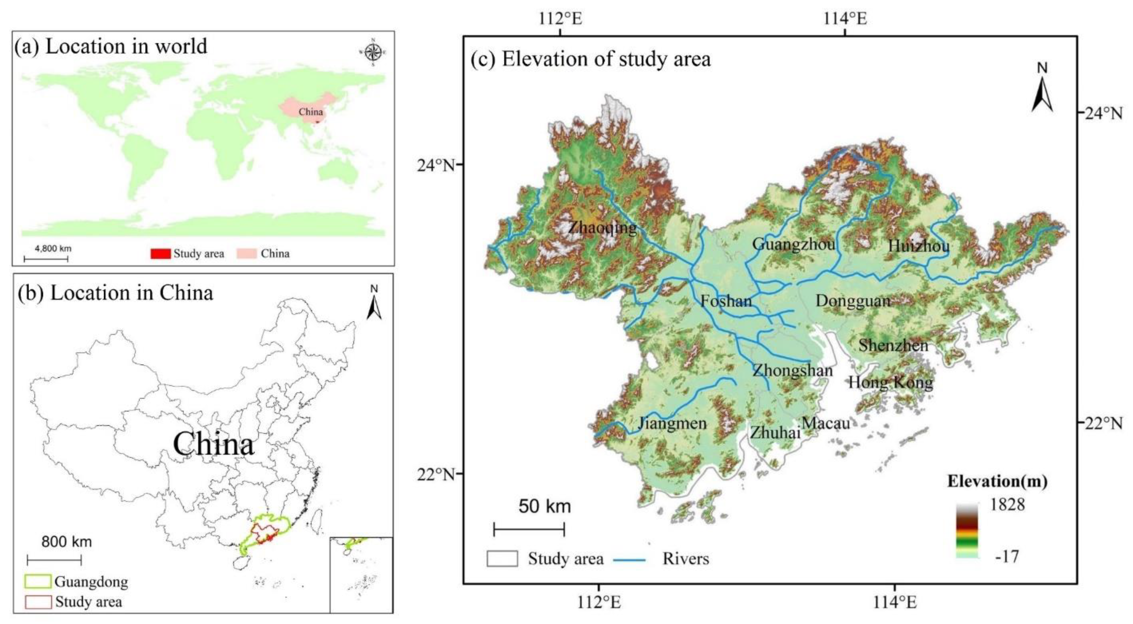
Figure 1. Location and elevation of the Guangdong–Hong Kong–Macao Greater Bay Area (GBA) in relation to (a) the world and (b) China, and (c) with elevation.
Remotesensing 13 01008 g001
Figure 2. Land cover/use in the GBA during the period from 1995 to 2015: (a) 1995, (b) 2000, (c) 2005, (d) 2010, (e) 2015.
Remotesensing 13 01008 g002
Figure 3. Data used in this study showing (a) the road network, and (b) industrial and residential areas in the GBA.
Remotesensing 13 01008 g003
Figure 4. Input data and processing steps to evaluate habitat quality in the Guangdong–Hong Kong–Macao Greater Bay Area (GBA). GDP—gross domestic product; POP—population distribution; PIS—proportion of impervious surface; FVC—fractional vegetation cover.
Remotesensing 13 01008 g004
Figure 5. The categories of variation in habitat quality. Note: +H: the high level of habitat quality increased; 0H: the high level of habitat quality did not change; −H: the high level of habitat quality decreased; +M: the moderate level of habitat quality increased; 0M: the moderate level of habitat quality did not change; −M: the moderate level of habitat quality decreased; +L: the low level of habitat quality increased; 0L: the low level of habitat quality did not change; −L: the low level of habitat quality decreased.
Remotesensing 13 01008 g005
Figure 6. Spatial distribution of habitat quality in the GBA during the period from 1995 to 2015: (a) 1995; (b) 2000; (c) 2005; (d) 2010; (e) 2015; the inset pie chart shows the proportions of each habitat quality range for different years.
Remotesensing 13 01008 g006
Figure 7. Numerical distribution of habitat quality for different ecosystem types: (a) 1995; (b) 2000; (c) 2005; (d) 2010; (e) 2015.
Remotesensing 13 01008 g007
Figure 8. The numerical distribution of habitat quality at different elevations in the years (a) 1995, (b) 2000, (c) 2005, (d) 2010, and (e) 2015.
Remotesensing 13 01008 g008
Figure 9. The variation in habitat quality in the Guangdong–Hong Kong–Macao Greater Bay Area (GBA) during the period from 1995 to 2015: (a) 1995 to 2000; (b) 2000 to 2005; (c) 2005 to 2010; (d) 2010 to 2015. Note: +H: the high level of habitat quality increased; 0H: the high level of habitat quality did not change; −H: the high level of habitat quality decreased; +M: the moderate level of habitat quality increased; 0M: the moderate level of habitat quality did not change; −M: the moderate level of habitat quality decreased; +L: the low level of habitat quality increased; 0L: the low level of habitat quality did not change; −L: the low level of habitat quality decreased.
Remotesensing 13 01008 g009
Figure 10. Area of built-up areas and forest land: (a) the percentage of built-up land; (b) the percentage of forest land.
Remotesensing 13 01008 g010
Table 1. The datasets and resources used in this study.
No.DatasetsData DescriptionData ResourcesData Format
1Land use/cover datasetsChina land use/cover change dataObtained from Resources and Environmental Sciences, Chinese Academy of Sciences (RESDC), http://www.resdc.cn, DataID = 184 (accessed on 20 January 2021)TIFF
2Vector datasetsRoad network datasets, residential datasets and industry datasets obtainedObtained from OpenStreetMap (OSM), https://download.geofabrik.de/ (accessed on 20 January 2021)Shapefile
3Socioeconomic datasetsPopulation distribution (POP) data Obtained from Oak Ridge National Laborator LandScan global population distribution data, https://landscan.ornl.gov/landscan-datasets (accessed on 20 January 2021)TIFF
Gross domestic product (GDP) dataObtained from RESDC 1 km grid GDP data, http://www.resdc.cn/data.aspx?DATAID=252 (accessed on 20 January 2021)TIFF
4Impervious surface dataGlobal artificial impervious dataObtained from global artificial impervious area (GAIA) maps, http://data.ess.tsinghua.edu.cn/gaia.html (accessed on 20 January 2021)TIFF
5Normalized difference vegetation index dataMOD13Q1 16-day products and RESDC NDVI datasetObtained from Level-1 and Atmosphere Archive & Distribution System Distributed Active Archive Center (LAADS DAAC) (https://ladsweb.modaps.eosdis.nasa.gov/ (accessed on 20 January 2021)) and RESDC (http://www.resdc.cn/DOI/doi.aspx?DOIid=49 (accessed on 20 January 2021))TIFF
6Supplementary analysis datasetsDEM datathe Shuttle Radar Topography Mission (SRTM), http://srtm.csi.cgiar.org/srtmdata/ (accessed on 20 January 2021)TIFF
Terrestrial ecosystem classification dataObtained from RESDC, http://www.resdc.cn/DOI/doi.aspx?DOIid=103 (accessed on 20 January 2021)TIFF
Table 2. The parameters of the habitat quality model.
ParameterParameter DescriptionData ResourcesData Format
LULCLand use/cover mapCNLUCCTIFF
Threat factorThe layer of threat factorOSM and CNLUCCTransferred to TIFF
Threat factor parametersThe weight of threat factorBased on relevant literature [4,27,30,31] and InVEST user’s guide [25]CSV
The maximum distance of each threat factor
The types of decay over space for the threat
Habitat suitability scoreEach LULC type needs to give a habitat suitability score with a value ranging from 0 to 1Based on relevant literature [4,27] and InVEST user’s guide [25]CSV
Sensitivity of habitat types to threat factorsThe parameter of the sensitivity score for LULC to the threat factorThe absolute value of Kendall’s correlation coefficientsCSV
Table 3. Threat factor parameter settings.
ThreatWeightMaximum DistanceDecay Type
Bare land0.23linear
Built-up areas110exponential
Cropland 0.688linear
Railway 0.99exponential
Trunk road110exponential
Primary road18linear
Secondary road0.755linear
Industry activity112exponential
Residential 0.55exponential
Table 4. Habitat suitability of each land use/land cover (LULC) type.
LULC TypesCroplandForestGrasslandWater BodiesWetlandBuilt-Up AreasUnused Land
Habitat score0.3510.40.9100
Table 5. Pearson’s correlation coefficients of habitat quality in relation to POP, PIS, GDP and FVC.
YearEffect Factors
GDPPOPPISFVC
1995−0.27 **−0.24 **−0.24 **0.47 **
2000−0.29 **−0.29 **−0.23 **0.51 **
2005−0.38 **−0.17 **−0.28 **0.48 **
2010−0.44 **−0.22 **−0.25 **0.5
2015−0.31 **−0.35 **−0.25 **0.48 **
Mean−0.34−0.26−0.250.49
Note: ** Correlation is significant at the 0.01 level (two-tailed); GDP—gross domestic product; POP—population distribution; PIS—proportion of impervious surface; FVC—fractional vegetation cover.
Publisher’s Note: MDPI stays neutral with regard to jurisdictional claims in published maps and institutional affiliations.