
Rangeland Fractional Components Across the Western United States from 1985 to 2018

 , , and
Abstract
1. Introduction
2. Materials and Methods
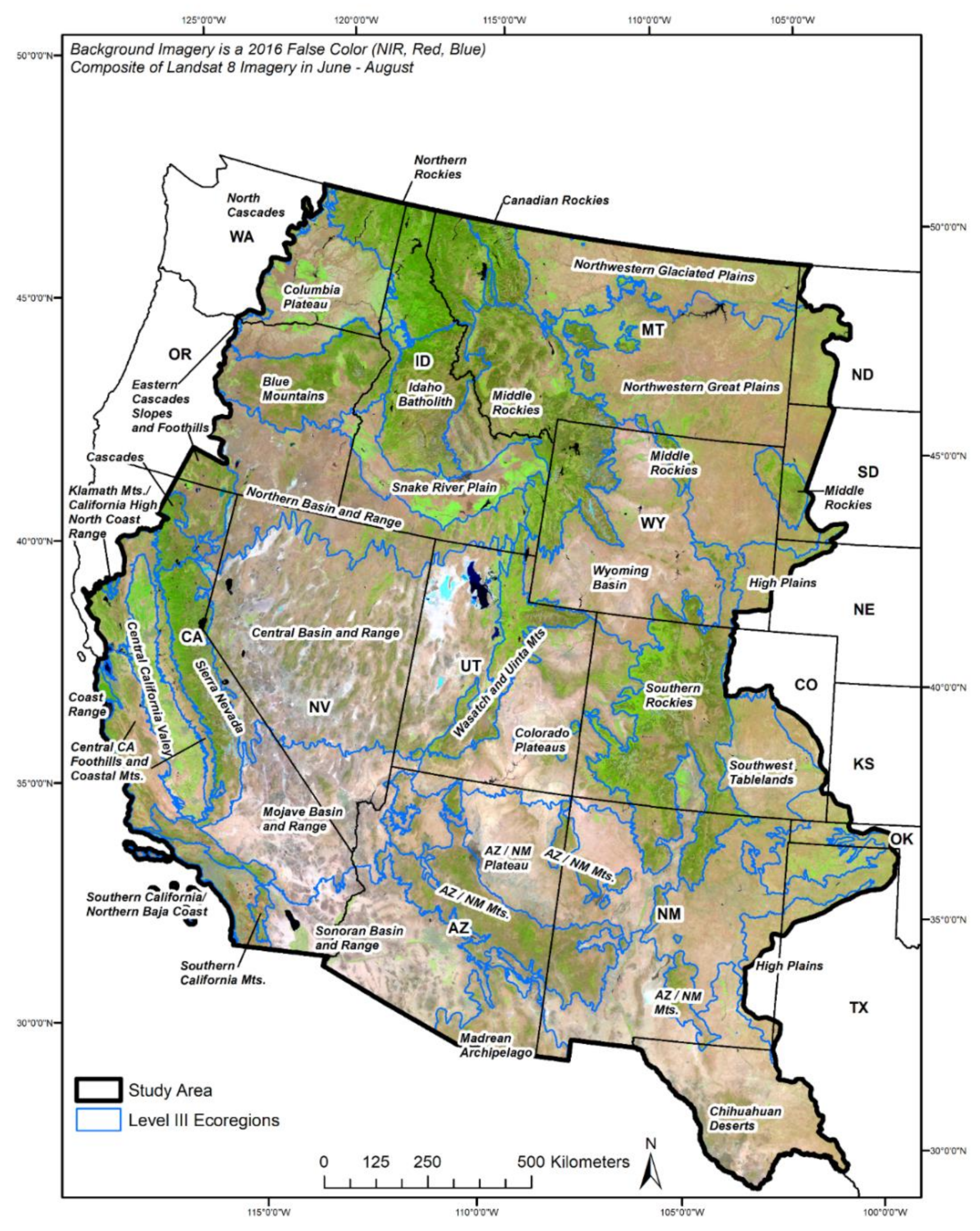
2.1. Study Area
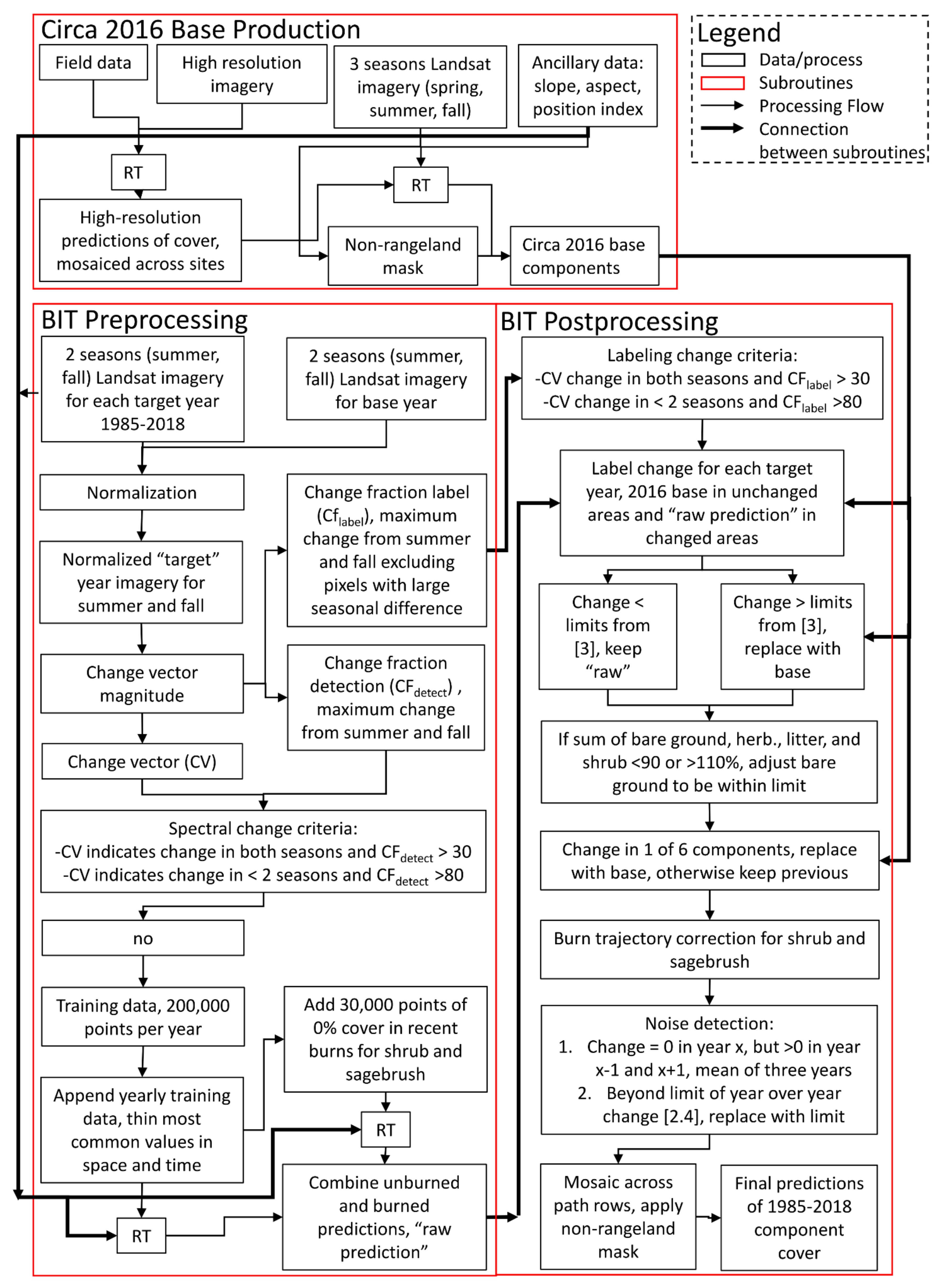
2.2. Method Overview
2.3. Base Map-Training Data Development
2.4. BIT Process
2.4.1. Image Processing
2.4.2. Ancillary Data
2.4.3. Land Cover Masking
2.4.4. Normalization
2.4.5. Change Detection
2.4.6. Training
2.4.7. Component Prediction
2.4.8. Change Labeling
2.5. Post Processing
2.6. Mosaicking
2.7. Validation
2.8. Trends Analysis
2.9. Statistics and Case Study Methods
3. Results
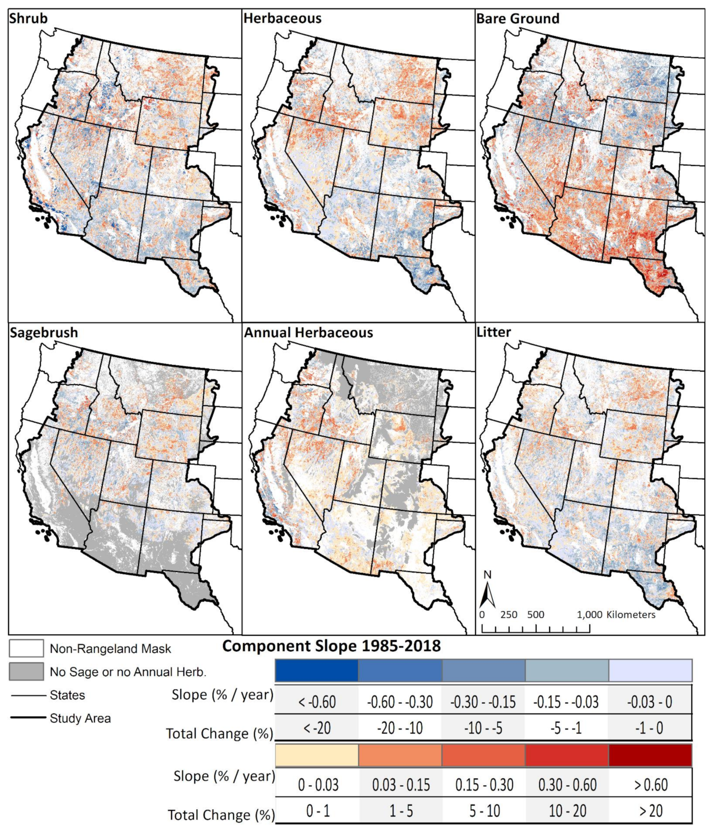
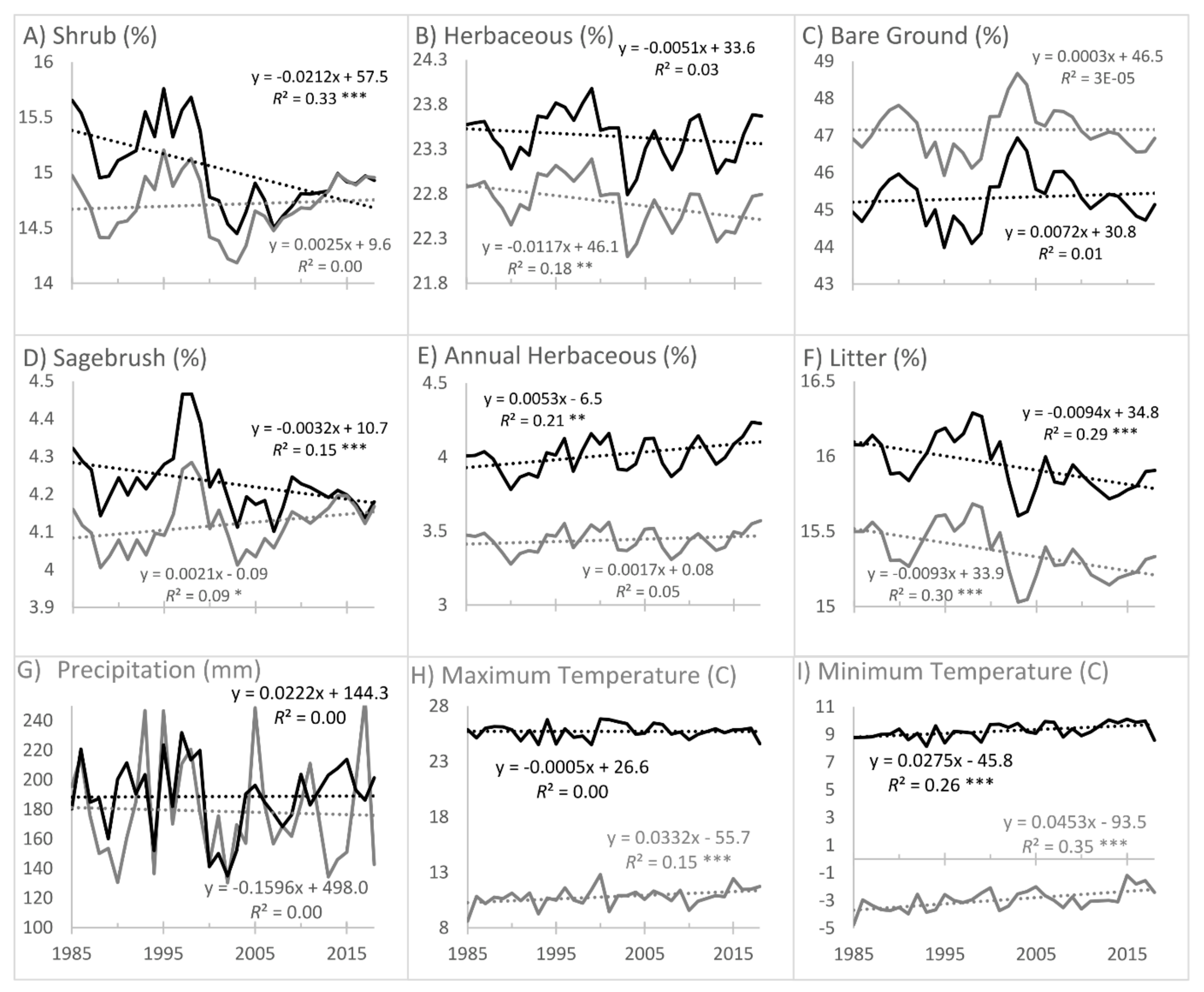
3.1. Overall Trends
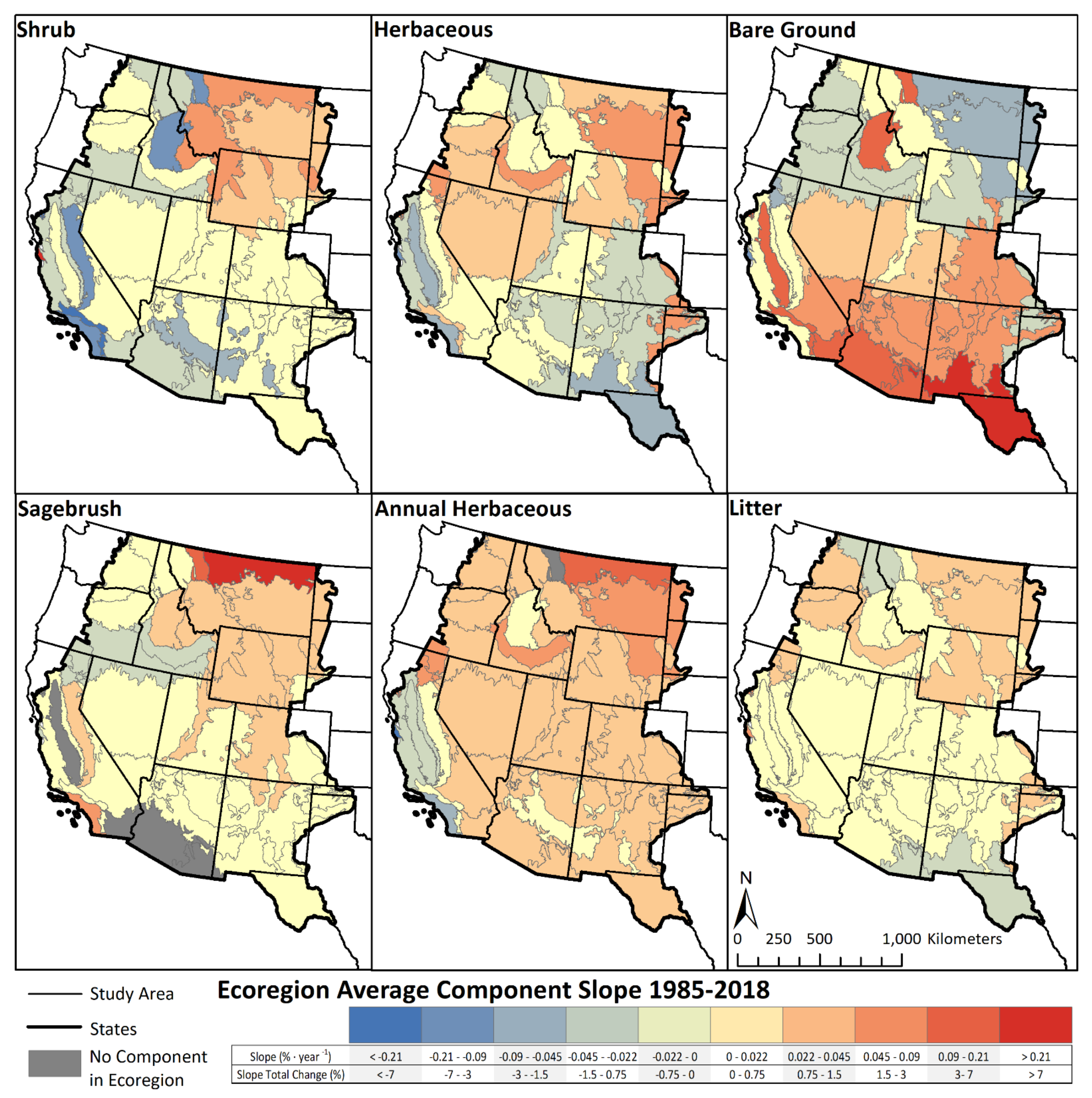
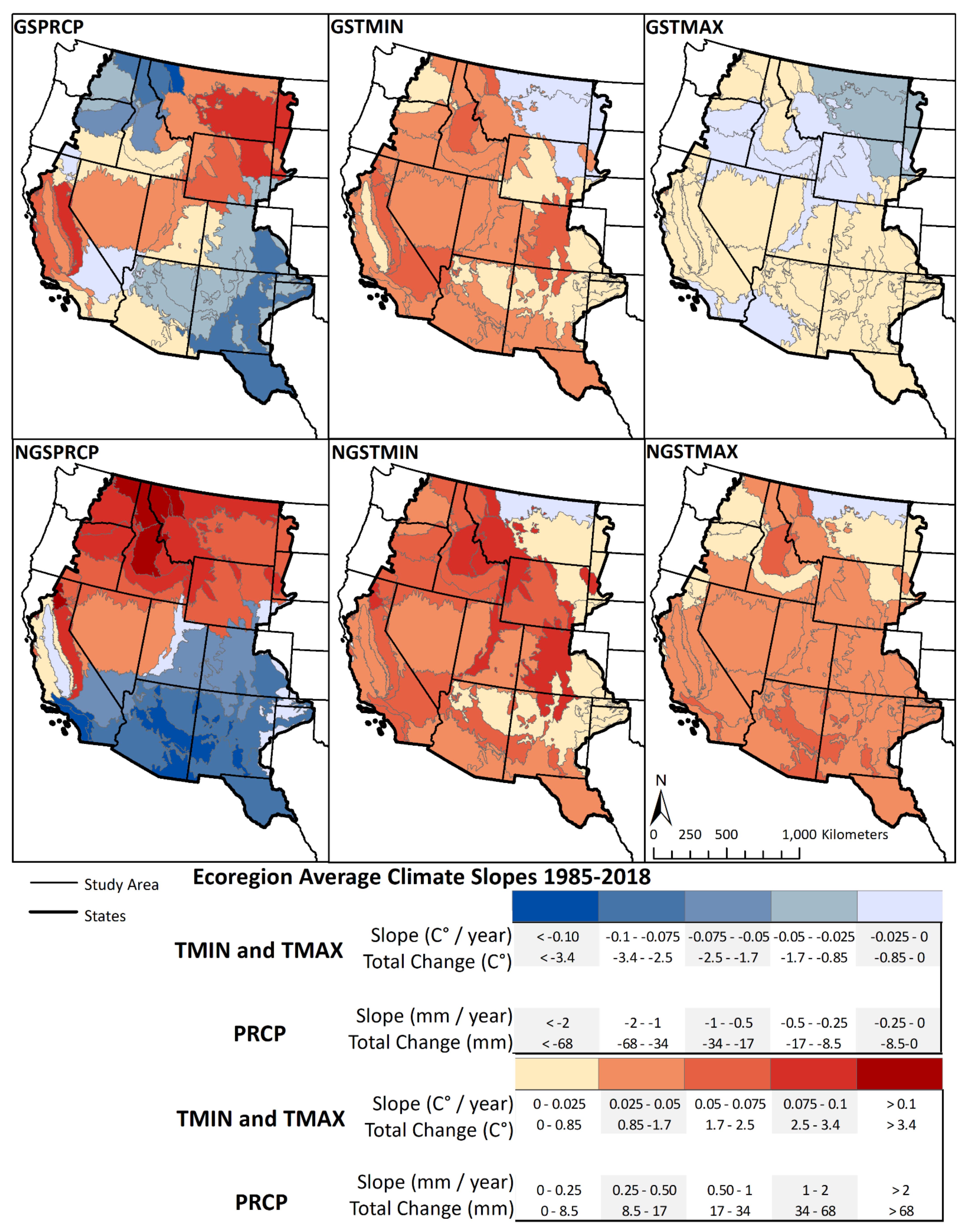
3.2. Level III Ecoregion Trends
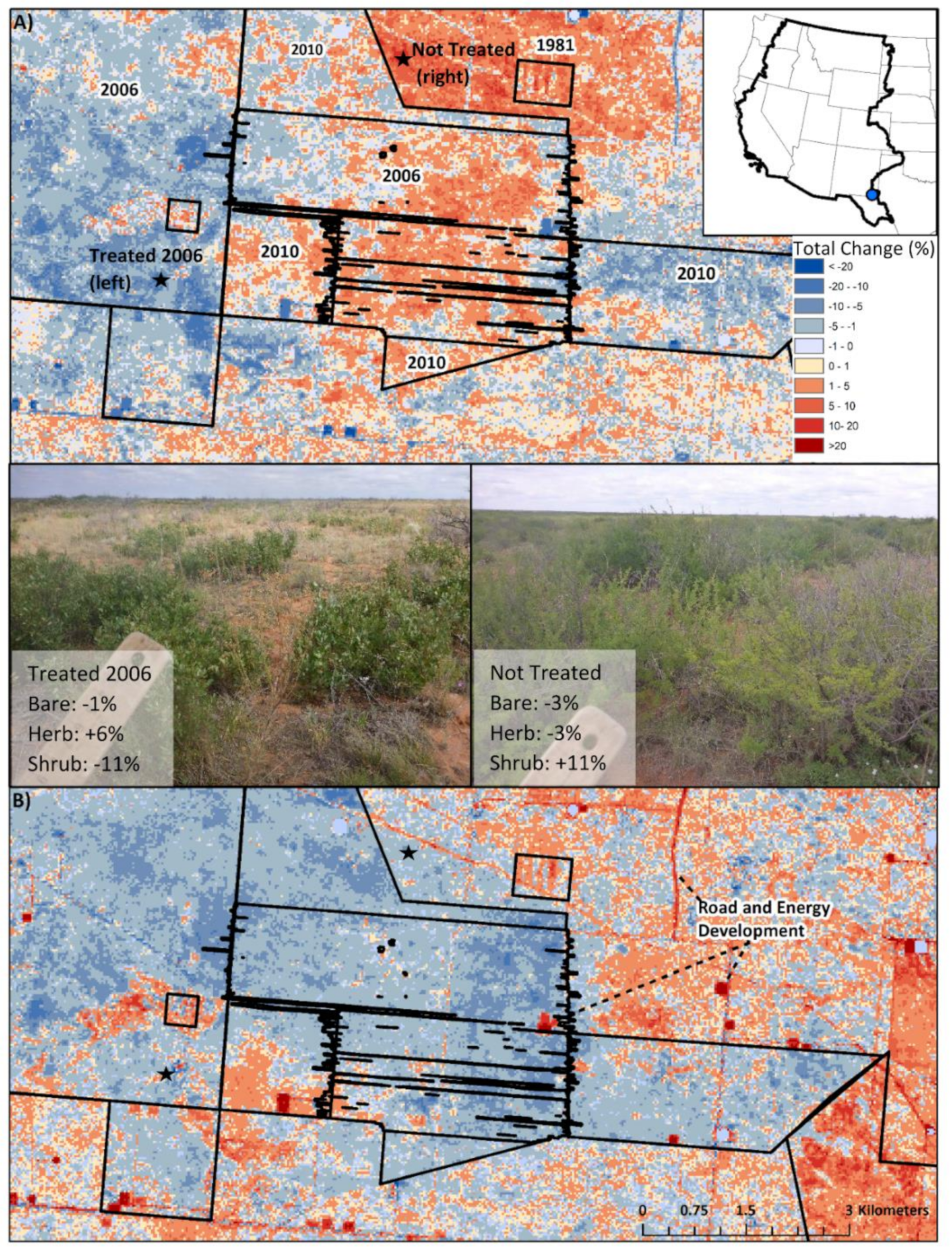
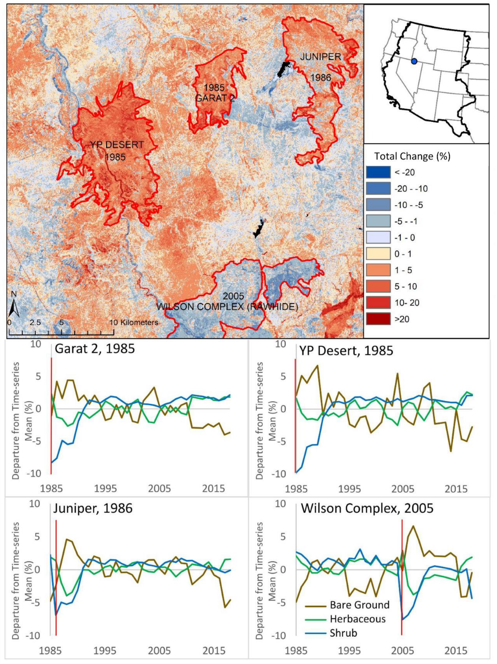
3.3. Case Studies
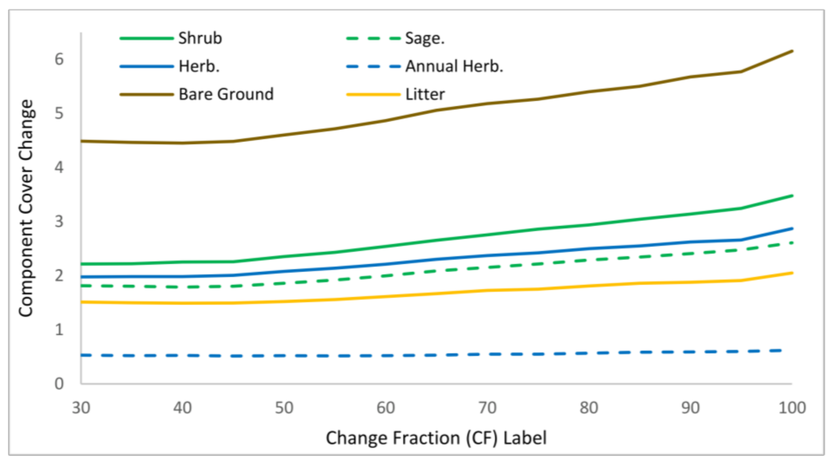
3.4. Change Fraction Sensitivity
4. Discussion
4.1. Ecoregion Level Trends
4.2. Going Forward
5. Conclusions
Supplementary Materials
Author Contributions
Funding
Informed Consent Statement
Data Availability Statement
Acknowledgments
Conflicts of Interest
References
- Sims, P.L.; Singh, J.S. The structure and function of ten western North American grasslands: III. Net primary production, turnover and efficiencies of energy capture and water use. J. Ecol. 1978, 66, 573–597. [Google Scholar] [CrossRef]
- Khumalo, G.; Holechek, J.; Thomas, M.; Molinar, F. Long-term vegetation productivity and trend under two stocking levels on Chihuahuan Desert rangeland. Rangeland Ecol. Manag. 2007, 60, 165–171. [Google Scholar] [CrossRef]
- Rigge, M.; Shi, H.; Homer, C.; Danielson, P.; Granneman, B. Long-term trajectories of fractional component change in the Northern Great Basin, USA. Ecosphere 2019, 10, e02762. [Google Scholar] [CrossRef]
- Williams, A.P.; Cook, E.R.; Smerdon, J.E.; Cook, B.I.; Abatzoglou, J.T.; Bolles, K.; Baek, S.H.; Badger, A.M.; Livneh, B. Large contribution from anthropogenic warming to an emerging North American megadrought. Science 2020, 368, 314–318. [Google Scholar] [CrossRef] [PubMed]
- Zhou, B.; Okin, G.; Zhang, J. Leveraging google earth engine (GEE) and machine learning algorithms to incorporate in situ measurement from different times for rangelands monitoring. Remote Sens. Environ. 2020, 236, 111521. [Google Scholar] [CrossRef]
- Jones, M.O.; Allred, B.W.; Naugle, D.E.; Maestas, J.D.; Donnelly, P.; Metz, L.J.; Karl, J.; Smith, R.; Bestelmeyer, B.; Boyd, C.; et al. Innovation in rangeland monitoring: Annual, 30 m, plant functional type percent cover maps for US rangelands, 1984–2017. Ecosphere 2018, 9, e0243. [Google Scholar] [CrossRef]
- Brown, J.; Tollerud, H.; Barber, C.; Zhou, Q.; Dwyer, J.; Vogelmann, J.; Loveland, T.; Woodcock, C.; Stehman, S.; Zhu, Z.; et al. Lessons learned implementing an operational continuous United States national land change monitoring capability: The Land Change Monitoring, Assessment, and Projection (LCMAP) approach. Remote Sens. Environ. 2020, 238, 111356. [Google Scholar] [CrossRef]
- Maynard, J.J.; Karl, J.W.; Browning, D.M. Effect of spatial image support in detecting long-term vegetation change from satellite time series. Landscape Ecol. 2016, 31, 2045–2062. [Google Scholar] [CrossRef]
- Woodcock, C.E.; Loveland, T.R.; Herold, M.; Bauer, M.E. Transitioning from change detection to monitoring with remote sensing: A paradigm shift. Remote Sens. Environ. 2020, 238, 111558. [Google Scholar] [CrossRef]
- Vogelmann, J.E.; Xian, G.; Homer, C.; Tolk, B. Monitoring gradual ecosystem change using Landsat time series analyses: Case studies in selected forest and rangeland ecosystems. Remote Sens. Environ. 2012, 122, 92–105. [Google Scholar] [CrossRef]
- Shi, H.; Rigge, M.; Homer, C.; Xian, G.; Meyer, D.; Bunde, B. Historical cover trends in a sagebrush steppe ecosystem from 1985 to 2013: Links with climate, disturbance, and management. Ecosystems 2017, 21, 913–929. [Google Scholar] [CrossRef]
- Rigge, M.; Homer, C.; Shi, H.; Meyer, D. Validating a Landsat time-series of fractional component cover across western U.S. rangelands. Remote Sens. 2019, 11, 3009. [Google Scholar] [CrossRef]
- Shi, H.; Homer, C.; Rigge, M.; Postma, K.; Xian, G. Assessing fractional component change in a shrubland ecosystem with both long-term field observations and a Landsat time-series in Wyoming USA. Ecosphere 2020, 11, e03311. [Google Scholar] [CrossRef]
- Rigge, M.; Homer, C.; Cleeves, L.; Meyer, D.; Bunde, B.; Shi, H.; Xian, G.; Bobo, M. Quantifying Western U.S. Rangelands as Fractional Components with Landsat. Remote Sens. 2020, 12, 412. [Google Scholar] [CrossRef]
- Omernik, J.M.; Griffth, G.E. Ecoregions of the conterminous United States: Evolution of a hierarchical spatial framework. Environ. Manag. 2014, 54, 1249–1266. [Google Scholar] [CrossRef]
- Jeffries, M.I.; Finn, S.P. The Sagebrush Biome Range Extent, as Derived from Classified Landsat Imagery: U.S. Geological Survey Data Release. Available online: https://www.sciencebase.gov/catalog/item/5ccb4a64e4b09b8c0b7808a6 (accessed on 13 May 2019).
- RuleQuest Research. Cubist, Version 2.05; Rule-Quest Pty: St Ives, NSW, Australia, 2008. [Google Scholar]
- Daly, C.; Smith, J.W.; Smith, J.I.; McKane, R.B. High-resolution spatial modeling of daily weather elements for a catchment in the Oregon Cascade Mountains, United States. J. Appl. Meteorol. Clim. 2007, 46, 1565–1586. [Google Scholar] [CrossRef]
- Xian, G.; Homer, C.; Aldridge, C. Effects of land cover and regional climate variations on long-term spatiotemporal changes in sagebrush ecosystems. GISci. Remote Sens. 2012, 49, 378–396. [Google Scholar] [CrossRef]
- Wylie, B.K.; Pastick, N.J.; Picotte, J.J.; Deering, C.A. Geospatial data mining for digital raster mapping. GISci. Remote Sens. 2018, 56, 406–429. [Google Scholar] [CrossRef]
- Ellsworth, L.M.; Wrobleski, D.W.; Kauffman, J.B.; Reis, S.A. Ecosystem resilience is evident 17 years after fire in Wyoming big sagebrush ecosystems. Ecosphere 2016, 7, e01618. [Google Scholar] [CrossRef]
- Batchelor, J.L.; Ripple, W.J.; Wilson, T.M.; Painter, L.E. Restoration of riparian areas following the removal of cattle in the Northwestern Great basin. Environ. Manag. 2015, 55, 930–942. [Google Scholar] [CrossRef]
- Pilliod, D. Land Treatment Digital Library—A Dynamic System to Enter, Store, Retrieve, and Analyze Federal Land-Treatment Data (Ver. 1.1, August 2015): U.S. Geological Survey Fact Sheet 2009-3095. Available online: https://pubs.usgs.gov/fs/2009/3095/ (accessed on 20 October 2009).
- Wisdom, M.J.; Rowland, M.M.; Tausch, R.J. Effective management strategies for sage-grouse and sagebrush: A question of triage? Trans. N. Am. Wildl. Nat. Resour. Conf. 2005, 70, 206–227. [Google Scholar]
- Augustine, D.; Davidson, A.; Dickinson, K.; Van Pelt, B. Thinking like a grassland: Challenges and opportunities for biodiversity conservation in the Great Plains of North America. Rangeland Ecol. Manag. 2020. [Google Scholar] [CrossRef]
- Bromley, G.T.; Gerken, T.; Prein, A.F.; Stoy, P.C. Recent trends in the near-surface climatology of the Northern North American Great Plains. J. Clim. 2020, 33, 461–475. [Google Scholar] [CrossRef]
- Chen, M.; Parton, W.J.; Hartman, M.D.; Del Grosso, S.J.; Smith, W.K.; Knapp, A.K.; Lutz, S.; Derner, J.D.; Tucker, C.J.; Ojima, D.S.; et al. Assessing precipitation, evapotranspiration, and NDVI as controls of U.S. Great Plains plant production. Ecosphere 2019, 10, e02889. [Google Scholar] [CrossRef]
- Reeves, M.; Hanberry, B.; Wilmer, H.; Kaplan, N.; Lauenroth, W. An assessment of production trends on the Great Plains from 1984–2017. Rangeland Ecol. Manag. in press. [CrossRef]
- Brookshire, E.N.J.; Stoy, P.C.; Currey, B.; Finney, B. The greening of the Northern Great Plains and its biogeochemical precursors. Glob. Chang. Biol. 2020, 10, 5404–5413. [Google Scholar] [CrossRef]
- McIntosh, M.M.; Holechek, J.L.; Speigal, S.A.; Cibils, A.F.; Estell, R.E. Long-term declining trends in Chihuahuan Desert forage production in relation to precipitation and ambient temperature. Rangeland Ecol. Manag. 2019, 72, 976–987. [Google Scholar] [CrossRef]
- Asner, G.P.; Archer, S.; Huges, R.F.; Ansley, R.J.; Wessman, C.A. Net changes in regional woody vegetation cover and carbon storage in Texas drylands 1937–1999. Glob. Chang. Biol. 2003, 9, 316–335. [Google Scholar] [CrossRef]
- Hanna, S.K.; Fulgham, K.O. Post-fire vegetation dynamics of a sagebrush steppe community change significantly over time. Calif. Agric. 2015, 69, 36–42. [Google Scholar] [CrossRef]
- Pastick, N.J.; Dahal, D.; Wylie, B.K.; Parajuli, S.; Boyte, S.P.; Wu, Z. Characterizing land surface phenology and exotic annual grasses in dryland ecosystems using Landsat and Sentinel-2 data in harmony. Remote Sens. 2020, 12, 725. [Google Scholar] [CrossRef]
- Maestas, J.; Jones, M.; Pastick, N.J.; Rigge, M.B.; Wylie, B.K.; Garner, L.; Crist, M.; Homer, C.; Boyte, S.; Witacre, B. Annual Herbaceous Cover across Rangelands of the Sagebrush Biome. Available online: https://doi.org/10.5066/P9VL3LD5 (accessed on 26 May 2020).
- Homer, C.; Rigge, M.; Shi, H.; Meyer, D.; Bunde, B.; Granneman, B.; Postma, K.; Danielson, P.; Case, A.; Xian, G. Remote Sensing Shrub/Grass National Land Cover Database (NLCD) Back-in-Time (BIT) Products for the Western U.S. Available online: https://doi.org/10.5066/P9C9O66W (accessed on 18 June 2020).


| Linear Trend | Shrub | Sage. | Herb. | Annual Herb. | Bare Ground | Litter |
|---|---|---|---|---|---|---|
| Changed (%) | 98.1 | 58.8 | 97.2 | 98.5 | 98.9 | 97.5 |
| Decrease (p < 0.10) (%) | 26.7 | 14.8 | 22.2 | 12.6 | 20.9 | 24.5 |
| Increase (p < 0.10) (%) | 19.2 | 11.3 | 18.6 | 18.6 | 21.1 | 16.7 |
| Total (p < 0.10) change (%) | 45.9 | 26.1 | 40.9 | 31.2 | 42.0 | 41.3 |
| Ratio of decrease to increase | 1.39 | 1.31 | 1.19 | 0.68 | 0.99 | 1.47 |
| Change (p < 0.10) in burns (%) 1 | 22.3 | 23.4 | 18.6 | 33.8 | 17.3 | 18.5 |
| Range (% Cover) | Shrub | Sage. | Herb. | Annual Herb. | Bare Ground | Litter |
|---|---|---|---|---|---|---|
| 0 | 1.46 | 0.67 | 2.34 | 0.53 | 0.66 | 1.99 |
| 1 to 5 | 27.87 | 36.58 | 25.57 | 24.58 | 7.57 | 44.27 |
| 6–10 | 35.84 | 39.34 | 27.43 | 44.55 | 21.74 | 37.91 |
| 11–15 | 16.76 | 15.08 | 19.88 | 17.20 | 22.08 | 12.38 |
| 16–20 | 7.45 | 5.93 | 12.17 | 8.23 | 17.21 | 2.81 |
| 21–25 | 3.89 | 1.91 | 6.56 | 4.11 | 12.08 | 0.51 |
| 26–30 | 2.29 | 0.43 | 3.19 | 2.21 | 7.81 | 0.09 |
| 31–35 | 1.77 | 0.05 | 1.51 | 1.10 | 4.74 | 0.02 |
| >35 | 2.66 | 0.01 | 1.35 | 1.22 | 6.11 | 0.00 |
| Mean | 10.54 | 7.93 | 11.18 | 10.35 | 17.14 | 6.59 |
Publisher’s Note: MDPI stays neutral with regard to jurisdictional claims in published maps and institutional affiliations. |
© 2021 by the authors. Licensee MDPI, Basel, Switzerland. This article is an open access article distributed under the terms and conditions of the Creative Commons Attribution (CC BY) license (http://creativecommons.org/licenses/by/4.0/).
Share and Cite
Rigge, M.; Homer, C.; Shi, H.; Meyer, D.; Bunde, B.; Granneman, B.; Postma, K.; Danielson, P.; Case, A.; Xian, G. Rangeland Fractional Components Across the Western United States from 1985 to 2018. Remote Sens. 2021, 13, 813. https://doi.org/10.3390/rs13040813
Rigge M, Homer C, Shi H, Meyer D, Bunde B, Granneman B, Postma K, Danielson P, Case A, Xian G. Rangeland Fractional Components Across the Western United States from 1985 to 2018. Remote Sensing. 2021; 13(4):813. https://doi.org/10.3390/rs13040813
Chicago/Turabian StyleRigge, Matthew, Collin Homer, Hua Shi, Debra Meyer, Brett Bunde, Brian Granneman, Kory Postma, Patrick Danielson, Adam Case, and George Xian. 2021. "Rangeland Fractional Components Across the Western United States from 1985 to 2018" Remote Sensing 13, no. 4: 813. https://doi.org/10.3390/rs13040813
APA StyleRigge, M., Homer, C., Shi, H., Meyer, D., Bunde, B., Granneman, B., Postma, K., Danielson, P., Case, A., & Xian, G. (2021). Rangeland Fractional Components Across the Western United States from 1985 to 2018. Remote Sensing, 13(4), 813. https://doi.org/10.3390/rs13040813