Abstract
The Taiwan Bank (TB) is located in the southern Taiwan Strait, where the marine environments are affected by South China Sea Warm Current and Kuroshio Branch Current in summer. The bottom water flows upward along the edge of the continental shelf, forming an upwelling region that is an essential high-productivity fishing ground. Using trophic dynamic theory, fishery resources can be converted into primary production required (PPR) by primary production, which indicates the environmental tolerance of marine ecosystems. This study calculated the PPR of benthic and pelagic species, sea surface temperature (SST), upwelling size, and net primary production (NPP) to analyze fishery resource structure and the spatial distribution of PPR in upwelling, non-upwelling, and thermal front (frontal) areas of the TB in summer. Pelagic species, predominated by those in the Scombridae, Carangidae families and Trachurus japonicus, accounted for 77% of PPR (67% of the total catch). The benthic species were dominated by Mene maculata and members of the Loliginidae family. The upwelling intensity was the strongest in June and weakest in August. Generalized additive models revealed that the benthic species PPR in frontal habitats had the highest deviance explained (28.5%). Moreover, frontal habitats were influenced by NPP, which was also the main factor affecting the PPR of benthic species in all three habitats. Pelagic species were affected by high NPP, as well as low SST and negative values of the multivariate El Niño–Southern Oscillation (ENSO) index in upwelling habitats (16.9%) and non-upwelling habitats (11.5%). The composition of pelagic species varied by habitat; this variation can be ascribed to impacts from the ENSO. No significant differences were noted in benthic species composition. Overall, pelagic species resources are susceptible to climate change, whereas benthic species are mostly insensitive to climatic factors and are more affected by NPP.
1. Introduction
Located in the southern part of the Taiwan Strait (TS), the Taiwan Bank (TB) is characterized by sand dunes and shallow water (approximate depth 10–30 m). Three primary currents affect the waters around the TB: the Kuroshio Branch Current (KBC), South China Sea Warm Current (SCSC), and China Coastal Current (CCC). These currents are defined by the seasonal monsoons [1,2,3]. In summer, the northeastward surface currents of the SCSC and KBC bringing the warm, saline, and oligotrophic water from the SCS to the ECS, which are predominantly driven by wind, and the bottom currents flow upward from the continental slope, forming upwellings with vertical mixing of different layers’ water (Figure 1) [1,2,3,4,5]. The upwelling and thermal front regions near the southern edge of the TB span approximately 2500–3000 km2 and are clearly observable in summer [2,4,5]. Thermal fronts with characteristic shapes appear at fixed locations around the upwelling, where the sea surface temperatures (SSTs) are lower and primary production (PP) is higher than those in the surrounding waters [5,6]. Here, four different water masses (the diluted water, the Kuroshio water, the upwelling water, and the warm water from the South China Sea (SCS)) contribute to the formation of fronts [5]. The thermal fronts and orientations around TB upwelling correspond to cold fronts with characteristic shapes in the north and south of TB upwelling [6]. Furthermore, small and mesoscale eddies, filaments caused by the monsoons and KBC, which all have an effect on the larva species due to the dispersion and convergence of nutrients [7,8]. Through foraging behavior, the aggregative response of biological interactions links primary productivity and top predators. Finally, the distribution of fishery resources in the different fisheries is affected [9,10,11,12].
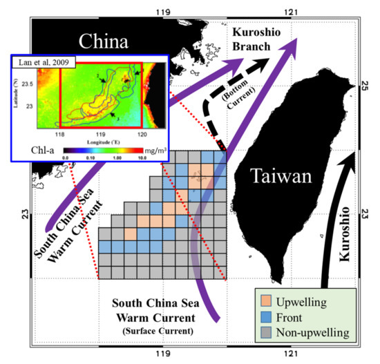
Figure 1.
Schematic of currents and three studied habitat types in the Taiwan Bank. The orange, blue, and gray boxes represent the upwelling, thermal front, and non-upwelling habitats, respectively.
High PP contributes to abundant fishery resources. The upwelling of nutrient-rich bottom water into the euphotic zone promotes the growth and propagation of phytoplankton, sustaining zooplankton communities and generally supporting fishery production. Therefore, upwelling strength directly affects the stability of marine ecosystems and general oceanic productivity [4,12,13]. Oceanic fronts (e.g., thermal fronts), sharp transition regions between water masses with disparate hydrographic, biological, or chemical properties, can limit the distribution of marine organisms, thereby serving as biogeographical boundaries [14,15,16]. The hydrographic characteristics of thermal fronts provide environmental conditions conducive to plankton blooms, fish aggregations, and consumer congregation [17,18]. Upwellings and thermal fronts have supported the maintenance of critical commercial fisheries near the TB since the 1950s; such fisheries typically employ light fishery, pole and line, and longline fishing, as well as trawling and gill nets [19]. The total catch weight and value of the offshore and coastal fisheries in the TS peaked in the 1980s, accounting for 44% of Taiwanese fishery production. By 2018, it had decreased to 16% (Figure 2). This dramatic decline can be attributed to high demand, unregulated fishing practices, and overexploitation [20,21]. In their evaluation of the stock status of 16 species under fishing pressure in the waters surrounding Taiwan, Ju et al. [21] discovered only one species that is not overfished. Furthermore, climate-driven environmental variabilities such as the El Niño–Southern Oscillation (ENSO) are pivotal factors affecting the intensity of the upwelling regions in the TB. The East Asian summer monsoon is always weaker at the peak of El Niño but strengthens when El Niño starts to decay [22,23,24]. This suggests that stronger south westerlies occur in the summer following an El Niño event and in turn more strongly promote coastal upwelling. In addition to warming the SCS currents northward, these winds produce higher SST gradients in the TS [12,25]. Changes in marine environments have also been demonstrated to affect fishery resources on different spatiotemporal scales, as well as ecological factors such as ecotourism and fisheries landings [26,27,28]. The marine environmental factors not only directly affect the habitat environment of biological preference but are also impactful on the competition and predation relationship of species in the ecosystem [27]. The bottom–up and top–down control could limit all the taxa in the ecosystem with interaction between species and the energy flow [29].
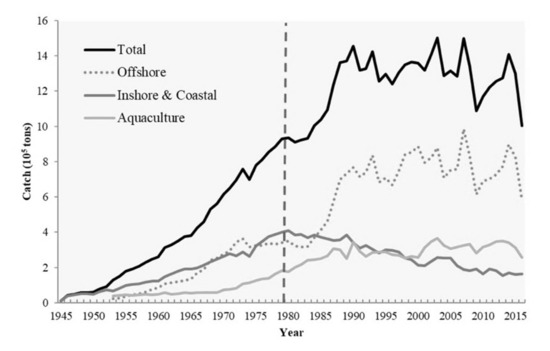
Figure 2.
Average annual catch of Taiwan Fishery from 1945 to 2017. The black line, dotted line, dark gray line and light gray line represent the total, offshore, inshore and coastal, and aquaculture fishery, respectively (Fisheries Agency, 2018).
PP, the basis for food chains, promotes the abundance of fishery resources [30,31,32]. Characterized by energy transfer between trophic levels, PP can be converted into percentages relative to the primary production required (PPR) to provide an estimate for the sustainability of fishery production [33]. In satellite telemetry studies, Chassot et al. [34] and Lam and Pauly [35] have found large marine ecosystems (LMEs) in tropical, temperate, and upwelling systems to have varying levels of fishery sustainability, trophic transfer efficiency, and species composition—all of which affect PPR. Watson et al. [36] investigated the historical operation of fishery fleets in major fishing grounds near six continents to gain an understanding of specific ecosystems and national fisheries, comparing their potential fishery sustainability. Knight and Jiang [37] used a fishing pressure index that compares NPP and PPR estimates for a specific catch to assess the sustainability of local fisheries in New Zealand and thereby provide a reference for subsequent fishery management. PPR can also be applied to large-scale fisheries, such as those in LMEs. Taken together, these studies indicate that PPR can reflect changes in fish catch that are related to energy flow; therefore, the interspecies transfer efficiency may accurately reflect the effect of ecosystems on fisheries.
Along with upwellings, the complexity of hydrological cycling and relevant changes that occur in summer are responsible for the high nutrient levels and high PP in the TB, a diverse fishing environment characterized by richness of species and habitats, which include upwelling, frontal, and non-upwelling habitats. However, studies on the TB have devoted little attention to differences in habitat characteristics when investigating the impacts of climate variability on PP and PPR in this region. Therefore, the present study collected data on fishery activity in the TB area and investigated the fishery resource structure and spatial distribution of PPR in upwelling, non-upwelling, and thermal front (frontal) habitats in summer. In addition, we explored the influence of marine climatic changes on the fishery resource structure and PPR of different habitat characteristics. The results are a valuable reference for ecosystem-based fishery management.
2. Materials and Methods
2.1. Fishery Data Collection
High spatial-resolution data on 11 types of fishery activity were collected from the voyage data recorders and logbooks of fishing vessels operating in the waters of the TB (118°E–120°E, 22°N–24°N) from 2011 to 2016 (Table 1). The fishery data comprised information on daily fishing locations for 0.1° spatial grids, including the fishing date, longitude and latitude, working hours (or soak time), total catch (catch weight in kg), and catch species.

Table 1.
The 12 pelagic and benthic species accounting for the highest proportion of total catch and primary production required in the Taiwan Bank region.
The life history strategies of fish differ by species, as do their environmental and habitat preferences. We used the Fish Database of Taiwan (http://fishdb.sinica.edu.tw/ (accessed on 5 January 2021)) and the FishBase database (http://www.fishbase.org (accessed on 5 January 2021)) to classify catch species as pelagic (living between the surface and bottom of the ocean) or benthic (comprising reef, demersal, and benthopelagic species).
2.2. Environmental Data and Climate Index
Daily SST data were extracted from images from the Advanced Very-High-Resolution Radiometer (AVHRR) cross-track scanning system developed by the US National Oceanic and Atmospheric Administration (NOAA). The AVHRR has a spatial resolution of 1.1 km, and the high-resolution picture transmissions are received at a ground station at National Ocean Taiwan University. Net primary production (NPP) data were estimated using the vertically generalized production model (VGPM) from the ocean productivity website of Oregon State University; the website is based on data from the Moderate Resolution Imaging Spectroradiometer (MODIS) Aqua, which has a spatial resolution of 9 km.
The ENSO, Western Pacific Oscillation (WPO), and Pacific Decadal Oscillation (PDO) are large-scale interannual and decadal climate variabilities that develop from air–sea interactions in the Pacific Ocean [38]. In this study, the ENSO was represented by the Oceanic Niño Index, which is based on a 3-month running mean of SST anomalies in the Niño 3.4 region (5°N–5°S, 120°W–170°W) between 1971 and 2000. We used the WPO index to represent the WPO event. Based on data from the NOAA Earth System Research Laboratories (ESRL; https://www.esrl.noaa.gov/psd/data/climateindices/list/ (accessed on 5 January 2021)), the WPO index is an indicator of changes in sea surface pressure in the western Pacific Ocean in winter; such changes affect the jet stream in the western and Central Pacific, altering water temperature and rainfall patterns [39]. The PDO was represented by the PDO index, the first empirical orthogonal function characterizing detrended SST anomalies in the Pacific north of 20°N [39]; PDO data were downloaded from the NOAA ESRL website.
2.3. Upwelling Size
The size of and variations in upwelling were estimated by examining the differences in water temperature between the upwelling and the non-upwelling regions. Upwelling regions were defined as regions with SSTs 1 °C to 3 °C lower than the monthly mean SST in the surrounding waters [1]. In images, each pixel represented 1.1 km2, and upwelling size was determined in accordance with the following equations used by Santos et al. [40]:
where is the upwelling strength of each longitude and latitude measured, is the SST at each longitude and latitude (°C), and is the mean SST of the study area (°C).
2.4. PPR and Contribution to PPR
To understand the PPR, characteristics of marine environments, and fishery resource structure in the waters around the TB, we gridded the monthly environmental and fishery data onto eighty 0.2° spatial grids. All 80 grids were classified by habitat type (upwelling, frontal, or non-upwelling) according to results reported by Lan et al. [6], who detected summertime upwelling and thermal front locations using long-term SST data (Figure 1).
PPR was used to reflect fishery catch in comparable energy units (t C·month−1) for the 0.2° spatial grids. PPR is the product of the carbon-converted catch weight and the conversion ratio for the trophic level of the taxa involved [36,41]:
where is the catch weight (ton), is the trophic transfer efficiency, and is the trophic level of species i.
The conversion of wet weight to carbon for the calculation of trophic transfer efficiency was based on a conservative 9:1 ratio [33,42]. Data of trophic level (TL) were extracted from FishBase.
Contribution to PPR is the percentage in PPR attributable to a single fish species. This contribution for a given year is calculated as follows:
where cPPRi is the percentage contribution of catch species i to overall PPR in year j, and PPRij is the PPR of species i in year j.
2.5. Statistical Models of Fishery Resources in Each Habitat
Generalized additive models (GAMs) were used to express the effects of environmental and climatic factors on the variations in the PPR of pelagic and benthic species in the three TB habitat types. The GAMs were constructed using the GAM function of the mgcv package in R [43]. A semiparametric approach to analyzing multiple nonlinear relationships between covariates and response variables, GAMs can also explain the variance in response variables [44]. In the present study, PPR was a response variable, and environmental (SST, NPP, and upwelling size) and climatic factors (multivariate ENSO index (MEI), WPO, and PDO) were the main independent variables (p < 0.05). The GAMs were constructed as follows:
where the constant c, which accounts for 10% of the mean of the overall observed PPR, was added to all PPR values because the log function cannot accept zeros; is the model constant; is a spline smoothing function for each model covariate . All covariates were continuous, and the number of effective degrees of freedom was estimated for each main factor. The optimal fitting model was selected through a stepwise procedure based on minimizing the Akaike information criterion (AIC). The residual distribution was used to evaluate model fit.
3. Results
3.1. Environment and Structure of Fishery Resources in TB Region
The spatial distribution of the monthly average SST and NPP in the TB region reveals that the areas of low SST and high NPP in summer closely overlap the upwelling grids, forming a banana shape (Figure 3). Overall, the SST was lower, and the upwelling size and NPP were higher in June and July than in August and September (Figure 4a). The greatest monthly variations in environmental factors occurred in the upwelling habitat, where the minimal SST ranged from 5.64 °C to 27.61 °C, maximal NPP ranged from 926.03 to 1273.86 mg·C·m−2·day−1, and upwelling area ranged from 136 to 194 km2 per grid (Figure 4b). The lowest SST and highest NPP were observed in frontal habitats in June also, but the upwelling spanned only 76 to 94 km2 per grid (Figure 4c). The non-upwelling habitats (Figure 4d) had the lowest NPP and upwelling size (6–20 km2 per grid).
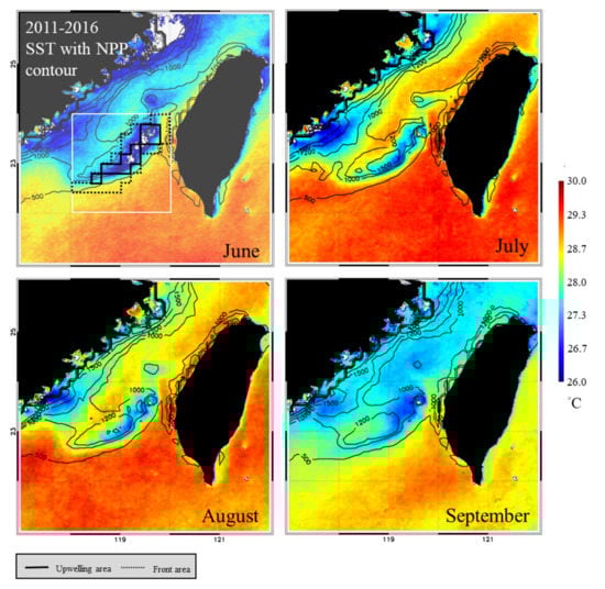
Figure 3.
Spatial distributions of monthly sea surface temperature (SST) and net primary production (NPP) in the Taiwan Bank region. The areas circumscribed by solid and dotted black lines are the upwelling and thermal front habitats, respectively.
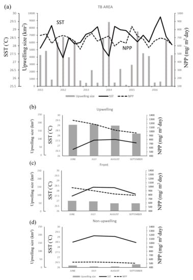
Figure 4.
Time series showing the relationship of sea surface temperature (SST) with net primary production (NPP) and upwelling size in (a) the Taiwan Bank (TB) region, (b) upwelling habitat, (c) thermal front habitat, and (d) non-upwelling habitat. Monthly data are presented in (b–d).
Data on 311 TB species, which are caught through various fishing methods, were recorded for the study period. Pelagic and benthic species, respectively, accounted for 67.09% and 28.99% of the total catch and 77.89% and 20.46% of the PPR (Table 1). Pelagic Scombridae species constituted the highest percentage of the total catch (30.90%) and PPR (37.00%). High cPPRs were also observed for Scomber australasicus (8.03%) and Auxis rochei (7.54%), both pelagic species (Table 1). The benthic species Mene maculata accounted for 9.90% of the total catch, but the cPPRs were 3.34%. None of each benthic species was higher than 5%.
3.2. Variations in Distribution of Fishery Resources and PPR
The PPR distributions of the pelagic and benthic species in the TB region differed during the study period (Figure 5). The PPR of pelagic species was the highest in the upwelling habitat and the northern part of the frontal habitat, as well as in the southeastern part of the non-upwelling habitat (Figure 5a). Benthic species with high PPR were observed mainly in the upwelling and frontal habitats and were both less abundant and more sparsely distributed in the non-upwelling habitat to the south (Figure 5b). Several species from the three habitats were selected for further comparison of the fishery resource structures and cPPR in the TB region. The pelagic representatives selected, Etrumeus micropus, Sardinella spp., Trachurus japonicus, Katsuwonus pelamis, Thunnus albacares, and Scombridae family. The selected benthic species are members of the Loliginidae family, as well as M. maculata and Trichiurus spp. The pelagic species from the Scombridae family and E. micropus had the highest cPPRs in the upwelling habitat, with successively lower contributions to PPR in the frontal and non-upwelling habitats (Figure 6). The cPPRs of T. japonicus, K. pelamis, and T. albacares were higher in the frontal and non-upwelling habitats. Benthic species from the Loliginidae family had higher cPPR in the upwelling and frontal habitats than in the non-upwelling habitat, and the cPPR of M. maculata was high (5.81%) in the non-upwelling habitat.
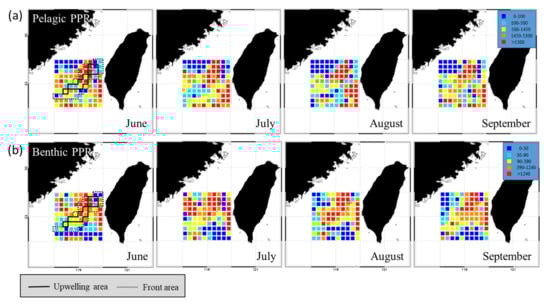
Figure 5.
Spatial distributions of monthly data for (a) pelagic primary production required (PPR) and (b) benthic PPR in the Taiwan Bank region (2011–2016). The areas circumscribed by solid and dotted black lines are the upwelling and thermal front habitats, respectively.
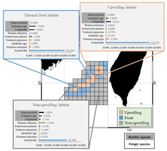
Figure 6.
The important species with the contributions to primary production required in the three habitats.
3.3. Effects of Environmental and Climatic Factors on PPR
The data used to select the benthic and pelagic species for GAM analysis are presented in Table 2 and Table 3. The maximal deviance explained of the selected benthic and pelagic species PPR was 28.5% and 22% in the frontal habitat (Table 2), 19.2% and 16.9% in the upwelling habitat, and 8.9% and 11.5% in the non-upwelling habitat. The NPP accounted for considerable portions of the variation in benthic species PPR in all three habitats, as well as that in the pelagic species in the frontal habitat (Table 3). Both SST and upwelling size were critical factors, explaining 6.41% and 6.83% of the deviance of the pelagic species PPR in the frontal habitat. Overall, the climatic factors of the MEI and PDO index were most strongly associated with the pelagic species PPR in the upwelling habitat (MEI: 10.10%) and the non-upwelling habitat (MEI: 4.74%, PDO: 5.26%).
Table 2.
Optimal models in each habitat by GAM analysis.
Table 3.
The deviance explained by each factor in each habitat GAM model.
A positive association was observed between the NPP and PPR of benthic and pelagic species in all habitats for NPP concentrations of 500–1500 mg·C·m−2·day−1 in all three habitats (Figure 7 and Figure 8). Monthly NPP peaked in June and decreased gradually through September for both species types in all three habitats, whereas monthly PPR increased gradually from June to August. These results indicate that the relationship between PPR and NPP may be time-lagged (Figure 9). Moreover, upwelling size and SST (27–29 °C) were positively associated with the benthic PPR in the frontal habitat (Figure 7c,d).
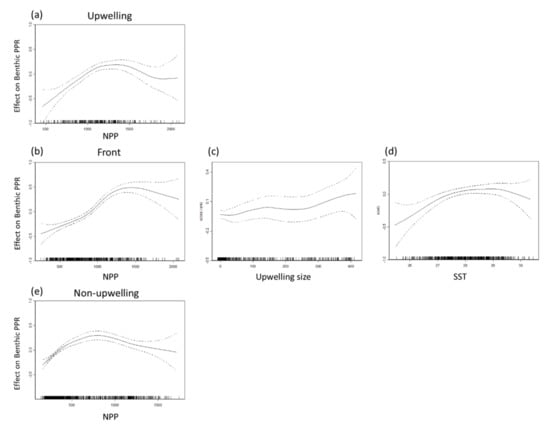
Figure 7.
Partial residual plots of the effects of each factor on benthic primary production required (PPR) in the (a) upwelling habitat, (b–d) thermal front habitat, and (e) non-upwelling habitat.
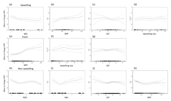
Figure 8.
Partial residual plots of the effects of each factor on pelagic primary production required (PPR) in the upwelling habitat (a–d), thermal front habitat (e–g), and non-upwelling habitat (h–k).
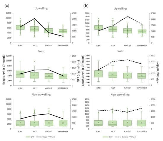
Figure 9.
Effects of net primary production (NPP; monthly means) on (a) pelagic primary production required (PPR), and (b) benthic PPR in the three habitats.
As shown in Figure 8, the MEI and PDO index were negatively associated with pelagic PPR in the upwelling and non-upwelling habitats, which revealed the differences in the characteristics of changes between years. The distribution of and differences in the annual summertime averages of the SST, NPP, and PPR of pelagic and benthic species during the negative (La Niña) and positive (El Niño) MEI events are presented in Figure 10. The annual summertime average time series indicate that pelagic PPR was highest in 2011 in La Niña year with higher NPP and relatively low in 2016 in El Niño year (Figure 10e). Otherwise, the relationships between benthic PPR and ENSO events were not clearly on time series patterns (Figure 10f).
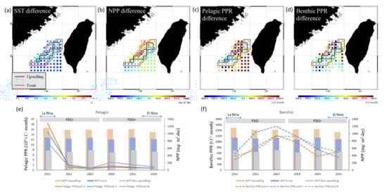
Figure 10.
Comparison of differences in the annual average (a) sea surface temperature (SST), (b) net primary production (NPP), (c) pelagic primary production required (PPR), and (d) benthic PPR in the Taiwan Bank region during the La Niña (2011) and El Niño (2016) events, as shown in spatial images and (e) Pelagic, and (f) Benthic PPR with NPP time series. The black and red boxes represent the upwelling and frontal habitats, respectively.
On the other hand, the difference of annual spatial distribution reveals that higher average PPRs were noted of pelagic species in the northwest and southeast parts of the frontal habitat, northern parts of the upwelling habitat, and southern parts of the non-upwelling habitat (Figure 10c), with lower SST (Figure 10a) and higher NPP (Figure 10b) in La Niña years. Variations in the spatial distribution of the PPR of benthic species were not associated with environmental factors during ENSO events (Figure 10d).
4. Discussion
4.1. Environmental Characteristics of Three TB Habitats
The monthly average data indicated that upwelling size and NPP were higher in June and July, and that in the waters around the TB, the SST, which is lower in summer, generally differs among the three habitats. For the summertime average SST difference between the upwelling habitat and fronts, non-upwelling is close to 0.7 and 1.5 °C, respectively. The SST was around 26 °C in TB upwelling, which was also within the SST ranges (24–26 °C) of upwelling areas shown in previous studies [1,3,6]. Furthermore, the SST gradient magnitudes of thermal front habitat calculated by Lan et al [6] were 0.1 to 0.2 °C/km and gradually disappeared in September. With other upwelling near TS, the average SST differences between upwelling and non-upwelling areas were 2 to 4 °C in the East China Sea and Dong Sheng upwelling [1,45].
Compared to Tang et al. [1], our results showing the difference of SST between upwelling and non-upwelling areas in TB presented the same patterns, which were approximately 1–3 °C, averaging 2.35 °C [1,46]. In September, as the SCSC and southwest monsoon weaken, the northeast monsoon and CCC begin to strengthen [6,47]. Lin et al. [48] discovered that rather than being closely correlated with variations in upwelling strength, wind direction and speed were mainly associated with topography, tides, and ocean currents [3,46,49]. The southwest monsoon drives the SCSC and KBC into the TS, causing the velocity of surface currents to exceed that of bottom currents [47,50]. SST increases gradually from upwelling areas to non-upwelling areas, and frontal habitats are affected by the upwelling of cold bottom water and downwelling of warm surface water [6,46,51], an effect that was strongest in July and weakest in September in this study.
The NPP, which also had different concentrations in three habitats, and NPP difference compared with upwelling habitats were closed to 238 and 590 mg·C·m−2·day−1 in thermal front and non-upwelling habitats, respectively. The monthly mean NPPs of MODIS Aqua calculated by VGPM were in the ranges of 500–1500 mg C m–2day–1 in TS [52]. The NPP ranges of China coastal upwelling is 600–2500 mg C m–2day–1; in Taiwan, northeastern upwelling is 500–1000 mg C m–2day–1 [52,53]. Rather SST or NPP in TB and other upwellings around TS present the obvious difference between upwelling and non-upwelling habitat. We suggest which could generalize into SST deviation at a lowest of 1°C and NPP deviation at a lowest of 500 mg C m–2day–1. These differences not only indicate the geography status but also show the impact of upwelling mechanism. The northeastern upwelling in TS was mainly caused by shelf break and wind stress curl; China coastal upwelling along TS was caused by alongshore winds, and TB upwelling was suggested to be caused by shelf break and background flow [3,7,23,45].
The NPP data indicated low nutrient concentrations in the non-upwelling area, whereas abundant nutrients such as phosphates and nitrates were present in the water upwelled from lower to upper layers or even to the surface layer [45,47]. Spatial distribution data suggest that the high PP, attributable to upwelling events and the accompanying nutritional richness, was responsible for the negative correlation between SST and NPP. In addition, in the first comparison of the satellite-derived VGPM estimates with in situ PP in the TS, Lan et al. [52] reported high correlation and low root-mean-square deviation. Satellite SST represents temperature only in the uppermost ocean layer and , being a function of SST, and differs in the lower layers, providing different photosynthetic efficiency [27]. The VGPM is one of the most widely known and applied depth-integrated/wavelength-integrated models. However, it has rarely been applied to coastal waters [54]. Thus, improvements in the accuracy of Chl-a from other ocean color sensors, including Medium Spectral Resolution Imaging Spectrometer and Ocean Color Climate Change Initiative data, will ultimately lead to an improvement in satellite PP algorithms for further research.
4.2. Fishery Resource Structure and PPR in Three TB Habitats
Both the fishing methods and fishery resource structure in the TB region are complex and variegated. The TS is located on the northern boundary of the Kuroshio triangle; it is characterized by high diversity of corals and reef species, and the currents and water depth create a suitable habitat for migratory species [55,56,57,58]. The distribution of top predators is dependent on that of anchovies and other forage species, which cluster in habitats located in thermal fronts [17]. Tiedemann and Brehmer [59] observed that larval and juvenile fish are divided into groups living in upwellings or thermal fronts. We noted that both fishery resource structure and PPR distributions in the TB differed by habitat.
In the present study, the upwelling habitat had high NPP and was dominated by cold-water pelagic species (i.e., E. micropus and Scombridae species) and benthic species (i.e., Loliginidae species). Attracted by the abundance of forage species, Scombridae species inhabit low-temperature areas with high NPP [60,61]. The main higher trophic level species (TL > 4.0) were Trichiurus spp. (TL = 4.42), followed by Loliginidae (TL = 4.0), Scombridae (TL = 4.0) and Etrumeus micropus (TL = 3.5). The Trichiurus spp. and Scombridae in TS main prey the Cephalopoda, which also prey small reef/demersal fish and small pelagic fish, respectively [62,63,64]. The species variations between three habitats were not only effected by the environment factors but also connected to the diet and feeding habits.
Furthermore, the PPR contributions of high trophic level species of Trichiurus spp. and Katsuwonus pelamis (TL = 4.03) were increased in the thermal front habitats, followed by Loliginidae, Etrumeus micropus and Trachurus japonicas (TL = 3.4). Tanabe [65] shows that the Trichiurus spp. and Loliginidae were the two main forage species of Katsuwonus pelamis. Trachurus japonicas is a small pelagic fish, and its diet is partially similar to Scombridae [66]. In the non-upwelling habitat, Thunnus albacares and Mene maculate express the higher composition, suggesting co-variation with the predator–prey relationships [67].
In addition, some tropical species such as T. albacares, Coryphaena hippurus, and K. pelamis appeared in the non-upwelling habitat. Chen [60] noted that the summer southwest monsoon causes a gradual rise in SST, and that upwelling periods characterized by high NPP correspond to the periods of the highest T. albacares and K. pelamis catches in non-upwelling habitats. In the present study, the fishery resource structure in the frontal habitat indicated that it is a transition zone between upwelling and non-upwelling habitats, a premise supported by the presence of both warm- and cold-water species, including E. micropus, K. pelamis, Scomberomorus commerson, T. japonicus, and Loliginidae species. Sabatini and Martos [17] and Sassa et al. [68] have reported that T. japonicus and Loliginidae species concentrate along the edge of thermal fronts. Wang et al. [69] found that frontal areas along northeastern Taiwan are dominated by immature fish from the Loliginidae family, whereas their adult counterparts appear in coastal waters and upwelling areas.
4.3. Explanatory Variables in GAM Analysis
The GAM analysis revealed that NPP accounted for a considerable portion of the variation in the benthic species in all three habitats, as well as that in the pelagic species in the frontal habitat. Moreover, the variation in PPR with NPP in the upwelling and frontal habitats may be time-lagged by 1 to 2 months. Higher NPP increases zooplankton blooms, directly increasing the first-level consumer resources [70,71]. Furthermore, the downstream secondary production creates an attractive habitat for species, such as those of the Scombridae and Loliginidae families and T. albacares, which occupy high trophic levels [28,53]. Therefore, the effect of high chlorophyll-a concentrations on NPP appears to be time-lagged because of trophic transfer efficiency [32,52,72,73]. Furthermore, the cPPR of benthic species was affected by variations in NPP. Studies have suggested that high spatiotemporal variability in NPP is positively correlated with demersal production [74,75]. The benthic PPR was not correlated with climate index but was highly positively correlated with NPP, indicating that its effects on NPP and upwelling events are asynchronous. Notably, the effects of dominant ENSO events on fishery catch were inconsistent. Furthermore, no relationships between the ENSO and NPP were noted. Tzeng et al. [76] observed that not all El Niño/La Niña events are similarly correlated with NPP in the eastern TS, stating that other factors may influence the spatial distribution of NPP. Wu et al. [77] inferred that the ENSO does not exert one single effect on summertime upwelling in the TS, and that the interaction between the East Asian monsoon systems in the China seas may play a role [78,79].
Our results indicate that pelagic PPR in the TB region is primarily affected by environmental and climatic factors. Song et al. [80] indicated that the SST is the factor most contributing to spawning–feeding migration in the TS. Ma et al. [81] reported that small pelagic species, including the chub mackerel and Pacific sardine, favor the low temperatures of the East China Sea. Climate variabilities have changed the marine environment in the TS; specifically, ENSO events influence the intensity of the upwelling in the TS [82]. The weaker wind field during El Niño events explains why summertime SST is higher during those events than during La Niña [12,25]. In essence, the changes in SST and upwelling intensity caused by climatic factors in the TB are the main factors affecting the migration patterns of the pelagic species in the three habitats.
4.4. Effects of Climate Change on the TB
The thermal fronts in the TB are characterized by two frontal belts on the northern and southern edges. Studies have indicated that the formation of the thermal front along the southern edge is linked to the interaction between topography and upwelling phenomena, whereas the thermal front along the northern edge may be tidally generated [51,83]. We compared the variations in the cPPR of pelagic and benthic species during El Niño and La Niña events (Table 4). During El Niño events, catches of Scombridae species decreased (Table 4), whereas catches of low-trophic-level species, such as E. micropus and Sardinella spp., increased. Moreover, pelagic PPR exhibited a trend of decline during these events (Figure 10). The cPPR of the pelagic species was higher during La Niña events, especially in the southern and northern part of the non-upwelling and upwelling habitats, respectively (Figure 10c). Moreover, cold-water species (Scombridae and Carangidae species and E. micropus) increased in abundance, as did warm-water species. Annual average time series obviously showed that the pelagic PPR was higher at La Nina (Figure 10e). The stronger El Niño event from 1997 to 1998 changed the dynamics of the summer monsoon and the mechanism of upwelling in the TS. Furthermore, it affected the composition and abundance of high-trophic-level pelagic species [25,78].
Table 4.
Contributions of individual species to primary production required in La Niña and El Niño years by habitat type.
The PDO has been shown to affect ocean productivity and eddy currents in the high- and mid-latitude regions of the North Pacific [76,84]. These effects are in turn associated with changes in marine ecosystems and fisheries [20,85,86]. The PDO index was a crucial factor in our GAM results, particularly those for the pelagic species in the upwelling and non-upwelling habitats. The WPO has been defined as a regional climate mode or subseasonal mode in which teleconnection patterns are expressed in a common region that has e–folding timescales between 7 and 10 days [87,88]. However, how the WPO alters climate patterns in the TS remains relatively unexplored. Baxter and Nigam [89] speculated that the WPO exerts stronger effects on air–sea flux in air pressure and rainfall. Thus, collecting more long-term fishery data and expanding the time scale on which the impacts of the PDO are investigated (i.e., beyond the decadal scale) are warranted in future research.
5. Conclusions
In the present analysis of fishery resource structure and the spatial distribution of PPR in upwelling, frontal, and non-upwelling habitats in the TB region in summer, variations in benthic PPR were correlated with changes in NPP. Members of the Loliginidae family, as well as M. maculata and Trichiurus spp., were the major benthic species in all three habitats. Variations in the pelagic PPR were influenced by ENSO events, and increased upwelling size contributed to lower SST and higher NPP in the TB region during La Niña events. High cPPR during La Niña events was observed for the pelagic species in the upwelling habitat, mainly those in the families of Scombridae (including A. rochei) and Carangidae. By contrast, during El Niño events, the dominant species were E. micropus and S. commerson. The frontal habitat marked the zone of transition between the two other habitats, and members of the Scombridae and Carangidae families and E. micropus had high cPPR in La Niña years. The high cPPR species during El Niño years were T. japonicus and K. pelamis. During La Niña events, the dominant pelagic species in the non-upwelling habitat were the same as those in the frontal habitat. During El Niño events, A. rochei rochei was the dominant species (Figure 11).
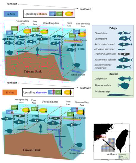
Figure 11.
The fishery resource structures on the three ecosystem habitats of Taiwan Bank in El Nino and La Nina year.
In the future, we hope to evaluate the performance of our models through various habitat classification methods. The global trend of sea temperature rise exerts substantial impacts on fisheries and ecosystems [77,90]. Shifts in environmental characteristics under the impacts of climate change mean that some habitats are no longer suitable for certain species; such impacts affect the entire ecosystem. The present research period spanned 6 years. To delineate the long-term relationship between climate change and the upwelling habitat in the TB, future studies should employ a longer study period.
Author Contributions
Conceptualization, K.-W.L.; methodology, K.-W.L. and P.-Y.H.; software, T.S.; formal analysis, K.-W.L. and M.-A.L.; resources, C.-H.L.; data curation, P.-Y.H., M.-A.L. and C.-H.L.; writing—original draft preparation, P.-Y.H.; writing—review and editing, P.-Y.H. and K.-W.L.; supervision, K.-W.L. All authors have read and agreed to the published version of the manuscript.
Funding
This research received no external funding.
Acknowledgments
This study was financially supported by the Council of Agriculture (109AS-1.1.5-ST-aC and 109AS-9.2.2-FA-F1(2)) and the National Science Council (MOST 108-2611-M-019-007 and MOST 109-2611-M-019-007). We are grateful to the Taiwan Ocean Conservation and Fisheries Sustainability Foundation for providing data from Taiwanese vessels. This manuscript was edited by Wallace Academic Editing. Finally, the authors thank anonymous reviewers for their constructive suggestions for improvement.
Conflicts of Interest
The authors declare no conflict of interest.
References
- Tang, D.L.; Kester, D.R.; Ni, I.H.; Kawamura, H.; Hong, H.S. Upwelling in the Taiwan Strait during the summer monsoon detected by satellite and shipboard measurements. Remote Sens. Environ. 2002, 83, 457–471. [Google Scholar] [CrossRef]
- Tang, D.L.; Kawamura, H.; Guan, L. Long-time observation of annual variation of Taiwan Strait upwelling in summer season. Adv. Space Res. 2004, 33, 307–312. [Google Scholar] [CrossRef]
- Jiang, Y.; Chai, F.; Wan, Z.; Zhang, X.; Hong, H. Characteristics and mechanisms of the upwelling in the southern Taiwan Strait: A three-dimensional numerical model study. J. Oceanogr. 2011, 67, 699–708. [Google Scholar] [CrossRef]
- Hu, J.; Kawamura, H.; Hong, H.; Pan, W. A review of research on the upwelling in the Taiwan Strait. Bull. Mar. Sci. 2003, 73, 605–628. [Google Scholar]
- Zhang, F.; Li, X.; Hu, J.; Sun, Z.; Zhu, J.; Chen, Z. Summertime sea surface temperature and salinity fronts in the southern Taiwan Strait. Int. J. Remote Sens. 2014, 35, 4452–4466. [Google Scholar] [CrossRef]
- Lan, K.W.; Kawamura, H.; Lee, M.A.; Chang, Y.; Chan, J.W.; Liao, C.H. Summertime sea surface temperature fronts associated with upwelling around the Taiwan Bank. Cont. Shelf Res. 2009, 29, 903–910. [Google Scholar] [CrossRef]
- Chang, Y.-L.; Miyazawa, Y.; Guo, X. Effect of mesoscale eddies on the Taiwan strait current. J. Phys. Oceanogr. 2015, 45, 1651–1666. [Google Scholar] [CrossRef]
- Zu, T.; Wang, D.; Yan, C.; Belkin, I.; Zhuang, W.; Chen, J. Evolution of an anticyclonic eddy southwest of Taiwan. Ocean Dyn. 2013, 63, 519–531. [Google Scholar] [CrossRef]
- Logerwell, E.A.; Smith, P.E. Mesoscale eddies and survival of late stage Pacific sardine (Sardinops sagax) larvae. Fish. Oceanogr. 2001, 10, 13–25. [Google Scholar] [CrossRef]
- Kai, E.T.; Marsac, F. Influence of mesoscale eddies on spatial structuring of top predators’ communities in the Mozambique Channel. Prog. Oceanogr. 2010, 86, 214–223. [Google Scholar]
- Zhou, C.; He, P.; Xu, L.; Bach, P.; Wang, X.; Wan, R.; Tang, H.; Zhang, Y. The effects of mesoscale oceanographic structures and ambient conditions on the catch of albacore tuna in the South Pacific longline fishery. Fish. Oceanogr. 2020, 29, 238–251. [Google Scholar] [CrossRef]
- Hong, H.; Chai, F.; Zhang, C.; Huang, B.; Jiang, Y.; Hu, J. An overview of physical and biogeochemical processes and ecosystem dynamics in the Taiwan Strait. Cont. Shelf Res. 2011, 31, S3–S12. [Google Scholar] [CrossRef]
- Wang, Y.; Kang, J.H.; Ye, Y.Y.; Lin, G.M.; Yang, Q.L.; Lin, M. Phytoplankton community and environmental correlates in a coastal upwelling zone along western Taiwan Strait. J. Mar. Syst. 2016, 154, 252–263. [Google Scholar] [CrossRef]
- McClain, C.R. A decade of satellite ocean color observations. Annu. Rev. Mar. 2009, 1, 19–42. [Google Scholar] [CrossRef]
- Stuart, V.; Platt, T.; Sathyendranath, S. Remote sensing and fisheries: An introduction. ICES J. Mar. Sci. 2011, 68, 639–641. [Google Scholar] [CrossRef]
- Klemas, V. Fisheries applications of remote sensing: An overview. Fish. Res. 2013, 148, 124–136. [Google Scholar] [CrossRef]
- Sabatini, M.; Martos, P. Mesozooplankton features in a frontal area off northern Patagonia (Argentina) during spring 1995 and 1998. Sci. Mar. 2002, 66, 215–232. [Google Scholar] [CrossRef]
- Malakoff, D. New tools reveal treasures at ocean hot spots: Biologically rich ocean “fronts” attract marine life—And could be candidates for conservation, too. Science 2004, 304, 1104–1106. [Google Scholar] [CrossRef]
- Chou, M.Y. Application Fishing Activity Data to Explore the Fishing Grounds Distribution Characteristics of Coastal Fisheries in Taiwan. Master’s Thesis, National Taiwan Ocean University, Keelung, Taiwan, 2017. [Google Scholar]
- Lan, K.W.; Zhang, C.I.; Kang, H.J.; Wu, L.J.; Lian, L.J. Impact of fishing exploitation and climate change on the grey mullet mugil cephalus stock in the Taiwan Strait. Mar. Coast. Fish. 2017, 9, 271–280. [Google Scholar] [CrossRef]
- Ju, P.; Tian, Y.; Chen, M.; Yang, S.; Liu, Y.; Xing, Q.; Sun, P. Evaluating stock status of 16 commercial fish species in the coastal and offshore waters of taiwan using the CMSY and BSM methods. Front. Mar. Sci. 2020, 7, 618. [Google Scholar] [CrossRef]
- Wang, Y.; Wang, B.; Oh, J.-H. Impact of the preceding El Niño on the East Asian summer atmosphere circulation. J. Meteorol. Soc. Jpn. Ser. II 2001, 79, 575–588. [Google Scholar] [CrossRef]
- Wen, C. Impacts of El Niño and La Niña on the cycle of the East Asian winter and summer monsoon. Chin. J. Atmos. Sci. 2002, 5, 359–376. [Google Scholar]
- Chen, W.; Feng, J.; Wu, R. Roles of ENSO and PDO in the link of the East Asian winter monsoon to the following summer monsoon. J. Clim. 2013, 26, 622–635. [Google Scholar] [CrossRef]
- Kuo, N.J.; Ho, C.R. ENSO effect on the sea surface wind and sea surface temperature in the Taiwan Strait. Geophys. Res. Lett. 2004, 31. [Google Scholar] [CrossRef]
- Bell, J.D.; Ganachaud, A.; Gehrke, P.C.; Griffiths, S.P.; Hobday, A.J.; Hoegh-Guldberg, O.; Johnson, J.E.; Le Borgne, R.; Lehodey, P.; Lough, J.M.; et al. Mixed responses of tropical Pacific fisheries and aquaculture to climate change. Nat. Clim. Chang. 2013, 3, 591–599. [Google Scholar] [CrossRef]
- Hazen, E.L.; Jorgensen, S.; Rykaczewski, R.R.; Bograd, S.J.; Foley, D.G.; Jonsen, I.D.; Shaffer, S.A.; Dunne, J.P.; Costa, D.P.; Crowder, L.B. Predicted habitat shifts of Pacific top predators in a changing climate. Nat. Clim. Chang. 2013, 3, 234–238. [Google Scholar] [CrossRef]
- Liao, C.H.; Lan, K.W.; Ho, H.Y.; Wang, K.Y.; Wu, Y.L. Variation in the catch rate and distribution of swordtip squid uroteuthis edulis associated with factors of the oceanic environment in the southern east China Sea. Mar. Coast. Fish. 2018, 10, 452–464. [Google Scholar] [CrossRef]
- Lynam, C.P.; Llope, M.; Möllmann, C.; Helaouët, P.; Bayliss-Brown, G.A.; Stenseth, N.C. Interaction between top-down and bottom-up control in marine food webs. Proc. Natl. Acad. Sci. USA 2017, 114, 1952–1957. [Google Scholar] [CrossRef] [PubMed]
- Valiela, I. Marine Ecological Processes; Springer: New York, NY, USA, 1995; p. 546. [Google Scholar]
- Howarth, R.W. Nutrient limitation of net primary production in marine ecosystems. Annu. Rev. Ecol. Evol. Syst. 1988, 19, 89–110. [Google Scholar] [CrossRef]
- Chassot, E.; Mélin, F.; Le Pape, O.; Gascuel, D. Bottom-up control regulates fisheries production at the scale of eco-regions in European seas. Mar. Ecol. Prog. Ser. 2007, 343, 45–55. [Google Scholar] [CrossRef]
- Pauly, D.; Christensen, V. Primary production required to sustain global fisheries. Nature 1995, 374, 255–257. [Google Scholar] [CrossRef]
- Chassot, E.; Bonhommeau, S.; Dulvy, N.K.; Mélin, F.; Watson, R.; Gascuel, D.; Le Pape, O. Global marine primary production constrains fisheries catches. Ecol. Lett. 2010, 13, 495–505. [Google Scholar] [CrossRef]
- Lam, V.W.; Pauly, D. Status of fisheries in 13 Asian Large Marine Ecosystems. Deep Sea Res. Part II Top. Stud. Oceanogr. 2019, 163, 57–64. [Google Scholar] [CrossRef]
- Watson, R.; Zeller, D.; Pauly, D. Primary productivity demands of global fishing fleets. Fish Fish. 2014, 15, 231–241. [Google Scholar] [CrossRef]
- Knight, B.R.; Jiang, W. Assessing primary production constraints in New Zealand fisheries. Fish. Res. 2009, 100, 15–25. [Google Scholar] [CrossRef]
- Mantua, N.J.; Hare, S.R. The Pacific decadal oscillation. J. Oceanogr. 2002, 58, 35–44. [Google Scholar] [CrossRef]
- Linkin, M.E.; Nigam, S. The North Pacific Oscillation–west Pacific teleconnection pattern: Mature-phase structure and winter impacts. J. Clim. 2008, 21, 1979–1997. [Google Scholar] [CrossRef]
- Santos, F.; Gomez-Gesteira, M.; Decastro, M.; Alvarez, I. Differences in coastal and oceanic SST trends due to the strengthening of coastal upwelling along the Benguela current system. Cont. Shelf Res. 2012, 34, 79–86. [Google Scholar] [CrossRef]
- Pauly, D.; Christensen, V.; Dalsgaard, J.; Froese, R.; Torres, F. Fishing down marine food webs. Science 1998, 279, 860–863. [Google Scholar] [CrossRef]
- Strathmann, R.R. Estimating the organic carbon content of phytoplankton from cell volume or plasma volume 1. Limnol. Oceanogr. 1967, 12, 411–418. [Google Scholar] [CrossRef]
- Wood, S.M. Generalized Additive Models, an Introduction with R; Chapman and Hall: London, UK, 2006; p. 392. [Google Scholar]
- Maunder, M.N.; Punt, A.E. Standardizing catch and effort data: A review of recent approaches. Fish. Res. 2004, 70, 141–159. [Google Scholar] [CrossRef]
- Hu, J.; Wang, X.H. Progress on upwelling studies in the China seas. Rev. Geophys. 2016, 54, 653–673. [Google Scholar] [CrossRef]
- Yan, T.Z.; Li, H.Y.; Yu, G.Y. Numerical study on upwelling along the coast of Fujian coastal, I. Three dimensional numerical simulation of upwelling in Taiwan Strait. Hai Yang Xue Bao 1997, 19, 12–19. [Google Scholar]
- Zhang, W.-Z.; Chai, F.; Hong, H.-S.; Xue, H. Volume transport through the Taiwan Strait and the effect of synoptic events. Cont. Shelf Res. 2014, 88, 117–125. [Google Scholar] [CrossRef]
- Lin, P.G.; Chen, Z.Z.; Hu, J.Y.; Zhu, J.; Sun, Z.Y. Variation characteristics of upwelling in Taiwan Strait and its relationship with wind in summer 2011. J. Oceanogr. Taiwan Strait 2012, 31, 307–316. [Google Scholar]
- Yan, Y.M.; Dai, C.S.; Lu, J.B. An inquisition of fisheries resources management in Taiwan Strait and its adjacent waters. J. Oceanogr. Taiwan Strait 2000, 19, 249–253. [Google Scholar]
- Huang, T.-H.; Lun, Z.; Wu, C.-R.; Chen, C.-T.A. Interannual carbon and nutrient fluxes in Southeastern Taiwan Strait. Sustainability 2018, 10, 372. [Google Scholar] [CrossRef]
- Chang, Y. High Resolution Satellite-Derived Sea Surface Temperature Front and Its Application on Fishery in the Taiwan Strait. Ph.D. Thesis, National Taiwan Ocean University, Keelung, Taiwan, 2009. [Google Scholar]
- Lan, K.W.; Chang, Y.J.; Wu, Y.L. Influence of oceanographic and climatic variability on the catch rate of yellowfin tuna (Thunnus albacares) cohorts in the Indian Ocean. Deep Sea Res. Part II Top. Stud. Oceanogr. 2020, 175, 104681. [Google Scholar] [CrossRef]
- Lan, K.W.; Lian, L.J.; Li, C.H.; Hsiao, P.Y.; Cheng, S.Y. Validation of a primary production algorithm of vertically generalized production model derived from multi-satellite data around the waters of Taiwan. Remote Sens. 2020, 12, 1627. [Google Scholar] [CrossRef]
- Tripathy, S.C.; Ishizaka, J.; Siswanto, E.; Shibata, T.; Mino, Y. Modification of the vertically generalized production model for the turbid waters of Ariake Bay, southwestern Japan. Estuar. Coast. Shelf Sci. 2012, 97, 66–77. [Google Scholar] [CrossRef]
- Chen, Y.Q.; Shen, X.Q. Changes in the biomass of the East China Sea Ecosystem. In Large Marine Ecosystems of the Pacific Rim Assessment, Sustainability and Management; Sherman, K., Tang, Q., Eds.; Blackwell Science: Malden, MA, USA, 1999; pp. 221–239. [Google Scholar]
- Talaue-McManus, L. Transboundary Diagnostic Analysis for the South China Sea; UNEP: Bangkok, Thailand, 2000; Volume 14. [Google Scholar]
- Qu, J.G.; Xu, Z.L.; Long, Q.; Wang, L.; Shen, X.; Zhang, J.; Cai, Y. East China Sea, GIWA Regional Assessment 36; University of Kalmar: Kalmar, Sweden, 2005; pp. 10–11. [Google Scholar]
- Wilkinson, C.C.; DeVantier, L.L.; Talau-McMaanus, L.L.; Souter, D.D. South China Sea, GIWA Regional Assessment 54; University of Kalmar: Kalmar, Sweden, 2005; pp. 9–11. [Google Scholar]
- Tiedemann, M.; Brehmer, P. Larval fish assemblages across an upwelling front: Indication for active and passive retention. Estuar. Coast. Shelf Sci. 2017, 187, 118–133. [Google Scholar] [CrossRef]
- Chen, Y.T. Studies on the Fishing-Oceanic Conditions of Taiwanese Seine Fishery in the Sorthwastern Waters of Taiwan. Master’s Thesis, National Taiwan Ocean University, Keelung, Taiwan, 2017. [Google Scholar]
- Kiyota, M.; Yonezaki, S.; Watari, S. Characterizing marine ecosystems and fishery impacts using a comparative approach and regional food-web models. Deep Sea Res. Part II Top. Stud. Oceanogr. 2020, 175, 104773. [Google Scholar] [CrossRef]
- Chiou, W.D.; Chen, C.Y.; Wang, C.M.; Chen, C.T. Food and feeding habits of ribbonfish Trichiurus lepturus in coastal waters of south-western Taiwan. Fish. Sci. 2006, 72, 373–381. [Google Scholar] [CrossRef]
- Sassa, C.; Tsukamoto, Y.; Konishi, Y. Diet composition and feeding habits of Trachurus japonicus and Scomber spp. larvae in the shelf break region of the East China Sea. Bull. Mar. Sci. 2008, 82, 137–153. [Google Scholar]
- Wang, Y.C.; Lin, L.P.; Sheng, Y.L.; Weng, J.S.; Lee, M.A. Stomach content analysis of Etrumeus micropus in the coastal waters of Penghu off Taiwan in late summer. J. Fish. Soc. Taiwan 2017, 44, 135–145. [Google Scholar]
- Tanabe, T. Feeding habits of skipjack tuna Katsuwonus pelamis and other tuna Thunnus spp. juveniles in the tropical western Pacific. Fish. Sci. 2001, 67, 563–570. [Google Scholar] [CrossRef]
- Fuita, T.; Kitagawa, D.; Okuyama, Y.; Ishito, Y.; Inada, T.; Jin, Y. Diets of the demersal fishes on the shelf off Iwate, northern Japan. Mar. Biol. 1995, 123, 219–233. [Google Scholar] [CrossRef]
- Weng, J.S.; Lee, M.A.; Liu, K.M.; Hsu, M.S.; Hung, M.K.; Wu, L.J. Feeding ecology of juvenile yellowfin tuna from waters southwest of Taiwan inferred from stomach contents and stable isotope analysis. Mar. Coast. Fish. 2015, 7, 537–548. [Google Scholar] [CrossRef]
- Sassa, C.; Tsukamoto, Y.; Nishiuchi, K.; Konishi, Y. Spawning ground and larval transport processes of jack mackerel Trachurus japonicus in the shelf-break region of the southern East China Sea. Cont. Shelf Res. 2008, 28, 2574–2583. [Google Scholar] [CrossRef]
- Wang, K.Y.; Liao, C.H.; Lee, K.T. Population and maturation dynamics of the swordtip squid (Photololigo edulis) in the southern East China Sea. Fish. Res. 2008, 90, 178–186. [Google Scholar] [CrossRef]
- Ware, D.M. Aquatic ecosystems: Properties and models. In Fisheries Oceanography: An Intrgrative Approach to Fisheries Ecology and Management; Harrison, P.J., Parsons, T.R., Eds.; Balckwell Science: Oxford, UK, 2000; pp. 161–200. [Google Scholar]
- Ware, D.M.; Thomson, R.E. Bottom-up ecosystem trophic dynamics determine fish production in the northeast pacific. Science 2005, 308, 1280–1284. [Google Scholar] [CrossRef] [PubMed]
- Yatsu, A.; Aydin, K.Y.; King, J.R.; McFarlane, G.A.; Chiba, S.; Tadokoro, K.; Kaeriyama, M.; Watanabe, Y. Elucidating dynamic responses of North Pacific fish populations to climatic forcing: Influence of life-history strategy. Prog. Oceanogr. 2008, 77, 252–268. [Google Scholar] [CrossRef]
- Ottersen, G.; Kim, S.; Huse, G.; Polovina, J.J.; Stenseth, N.C. Major pathways by which climate may force marine fish populations. J. Mar. Syst. 2010, 79, 343–360. [Google Scholar] [CrossRef]
- Van Denderen, P.D.; Hintzen, N.T.; Rijnsdorp, A.D.; Ruardij, P.; van Kooten, T. Habitat-specific effects of fishing disturbance on benthic species richness in marine soft sediments. Ecosystems 2014, 17, 1216–1226. [Google Scholar] [CrossRef]
- Buhl-Mortensen, L.; Ellingsen, K.E.; Buhl-Mortensen, P.; Skaar, K.L.; Gonzalez-Mirelis, G. Trawling disturbance on megabenthos and sediment in the Barents Sea: Chronic effects on density, diversity, and composition. ICES J. Mar. Sci. 2016, 73, i98–i114. [Google Scholar] [CrossRef]
- Tzeng, W.N.; Tseng, Y.H.; Han, Y.S.; Hsu, C.C.; Chang, C.W.; Di Lorenzo, E.; Hsieh, C.H. Evaluation of multi-scale climate effects on annual recruitment levels of the Japanese eel, Anguilla japonica, to Taiwan. PLoS ONE 2012, 7, e30805. [Google Scholar] [CrossRef]
- Wu, Y.L.; Lee, M.A.; Chen, L.C.; Chan, J.W.; Lan, K.W. Evaluating a suitable aquaculture site selection model for Cobia (Rachycentron canadum) during extreme events in the inner bay of the Penghu Islands, Taiwan. Remote Sens. 2020, 12, 2689. [Google Scholar] [CrossRef]
- Hong, H.S.; Shang, S.L.; Zhang, C.Y.; Huang, B.Q.; Hu, J.Y.; Huang, J.Q.; Lu, Z.B. Evidence of ecosystem response to the interannual environmental variability in the Taiwan Strait. Hai Yang Xue Bao 2005, 27, 63–69. [Google Scholar]
- Huang, Y.H. ENSO Effects on Marine Meteorology of Adjacent Waters Surrounding Taiwan. Master’s Thesis, National San Yet-sen University, Kaohsiung, Taiwan, 2005. [Google Scholar]
- Song, P.; Zhang, J.; Lin, L.; Xu, Z.; Zhu, X. Nekton species composition and biodiversity in Taiwan Strait. Sheng Wu Duo Yang Xing 2012, 20, 32–40. [Google Scholar]
- Ma, S.; Cheng, J.; Li, J.; Liu, Y.; Wan, R.; Tian, Y. Interannual to decadal variability in the catches of small pelagic fishes from China Seas and its responses to climatic regime shifts. Deep Sea Res. Part II Top. Stud. Oceanogr. 2019, 159, 112–129. [Google Scholar] [CrossRef]
- Yan, Y. Study on the relationship between the Sea Surface Temperature (SST) in NINO Region and the yield of pelagic fish in Minnan-Taiwan Bank Fishing Ground. J. Fujian Fish. 2006, 4, 11–15. [Google Scholar]
- Chang, Y.; Shimada, T.; Lee, M.A.; Lu, H.J.; Sakaida, F.; Kawamura, H. Wintertime sea surface temperature fronts in the Taiwan Strait. Geophys. Res. Lett. 2006, 33. [Google Scholar] [CrossRef]
- Tian, Y.; Kidokoro, H.; Watanabe, T.; Iguchi, N. The late 1980s regime shift in the ecosystem of Tsushima warm current in the Japan/East Sea: Evidence from historical data and possible mechanisms. Prog. Oceanogr. 2008, 77, 127–145. [Google Scholar] [CrossRef]
- Yasuda, I.; Sugisaki, H.; Watanabe, Y.; Minobe, S.S.; Oozeki, Y. Interdecadal variations in Japanese sardine and ocean/climate. Fish. Oceanogr. 1999, 8, 18–24. [Google Scholar] [CrossRef]
- Lan, K.W.; Lee, M.A.; Zhang, C.I.; Wang, P.Y.; Wu, L.J.; Lee, K.T. Effects of climate variability and climate change on the fishing conditions for grey mullet (Mugil cephalus L.) in the Taiwan Strait. Clim. Chang. 2014, 126, 189–202. [Google Scholar] [CrossRef]
- Barnston, A.G.; Livezey, R.E. Classification, seasonality and persistence of low-frequency atmospheric circulation patterns. Mon. Weather Rev. 1987, 115, 1083–1126. [Google Scholar] [CrossRef]
- Feldstein, S.B. The timescale, power spectra, and climate noise properties of teleconnection patterns. J. Clim. 2000, 13, 4430–4440. [Google Scholar] [CrossRef]
- Baxter, S.; Nigam, S. Key role of the North Pacific Oscillation–west Pacific pattern in generating the extreme 2013/14 North American winter. J. Clim. 2015, 28, 8109–8117. [Google Scholar] [CrossRef]
- Lee, M.A.; Kuo, Y.C.; Chan, J.W.; Chen, Y.K.; Teng, S.Y. Long-term (1982–2012) summertime sea surface temperature variability in the Taiwan Strait. Terr. Atmos. Ocean. Sci. 2015, 26, 183–192. [Google Scholar] [CrossRef]


Publisher’s Note: MDPI stays neutral with regard to jurisdictional claims in published maps and institutional affiliations. |
© 2021 by the authors. Licensee MDPI, Basel, Switzerland. This article is an open access article distributed under the terms and conditions of the Creative Commons Attribution (CC BY) license (http://creativecommons.org/licenses/by/4.0/).