Article

Neighbor-Based Label Distribution Learning to Model Label Ambiguity for Aerial Scene Classification

School of Mechanical Engineering, Southwest Jiaotong University, Chengdu 610031, China
*
Author to whom correspondence should be addressed.
Remote Sens. 2021, 13(4), 755; https://doi.org/10.3390/rs13040755
Submission received: 4 January 2021 / Revised: 13 February 2021 / Accepted: 16 February 2021 / Published: 18 February 2021

Abstract

:
Many aerial images with similar appearances have different but correlated scene labels, which causes the label ambiguity. Label distribution learning (LDL) can express label ambiguity by giving each sample a label distribution. Thus, a sample contributes to the learning of its ground-truth label as well as correlated labels, which improve data utilization. LDL has gained success in many fields, such as age estimation, in which label ambiguity can be easily modeled on the basis of the prior knowledge about local sample similarity and global label correlations. However, LDL has never been applied to scene classification, because there is no knowledge about the local similarity and label correlations and thus it is hard to model label ambiguity. In this paper, we uncover the sample neighbors that cause label ambiguity by jointly capturing the local similarity and label correlations and propose neighbor-based LDL (N-LDL) for aerial scene classification. We define a subspace learning problem, which formulates the neighboring relations as a coefficient matrix that is regularized by a sparse constraint and label correlations. The sparse constraint provides a few nearest neighbors, which captures local similarity. The label correlations are predefined according to the confusion matrices on validation sets. During subspace learning, the neighboring relations are encouraged to agree with the label correlations, which ensures that the uncovered neighbors have correlated labels. Finally, the label propagation among the neighbors forms the label distributions, which leads to label smoothing in terms of label ambiguity. The label distributions are used to train convolutional neural networks (CNNs). Experiments on the aerial image dataset (AID) and NWPU_RESISC45 (NR) datasets demonstrate that using the label distributions clearly improves the classification performance by assisting feature learning and mitigating over-fitting problems, and our method achieves state-of-the-art performance.

Graphical Abstract

1. Introduction

Aerial scene classification aims at classifying each aerial image into a scene label, which is typically cast as a single label learning (SLL) problem. Convolutional neural networks (CNNs) have been acknowledged as the most powerful approach for aerial scene classification [1,2]. The fact that some aerial scenes share similar appearance or objects causes the label ambiguity of aerial image. Some References [3,4,5] handle the label ambiguity through multi-label learning (MLL). Both SLL and MLL aim to answer the question ‘which label can describe the sample?’. Different from SLL or MLL, label distribution learning (LDL) [6,7] handles the more ambiguous question ‘how much does each label describe the sample?’. For a sample, its label distribution represents the degree to which each label describes the sample. In this way, samples are associated with multiple labels, and a sample can contribute to not only the learning of the ground truth, but also the learning of correlated labels. Thus, each label is supplied with more training data. Using label distributions to express label ambiguity can boost CNN learning by improving data utilization [7,8,9,10,11].

1.1. Difficulties in Modeling Label Ambiguity

However, the label distribution of each sample is unavailable in original training sets and needs to be constructed by modeling label ambiguity. It is generally known that label ambiguity is caused by those similar samples that have different but correlated labels [7]. Existing LDL methods are invalid for scene classification due to the following reasons:
  • The widely used label distribution is Gaussian smoothing from the sample ground truth to close labels [7,8,9,10,11], as shown in Figure 1. For the age images, local sample similarity is known, i.e., similar images have close ages; also, global label correlations are available, i.e., the age difference reflects label correlations. The Gaussian distribution properly models the label ambiguity because both the local similarity and label correlations are captured.
  • For scene classification or generic SLL problems, neither local similarity nor label correlations are known, and thus it is hard to model label ambiguity. As mentioned in Gao et al. [7], modeling label ambiguity is challenging due to the diversity of label space.

1.2. Motivation and Fundamental Ideal

Our goal is to construct label distributions for CNN training, which needs to model the label ambiguity regarding aerial images. Our motivation is as follows:
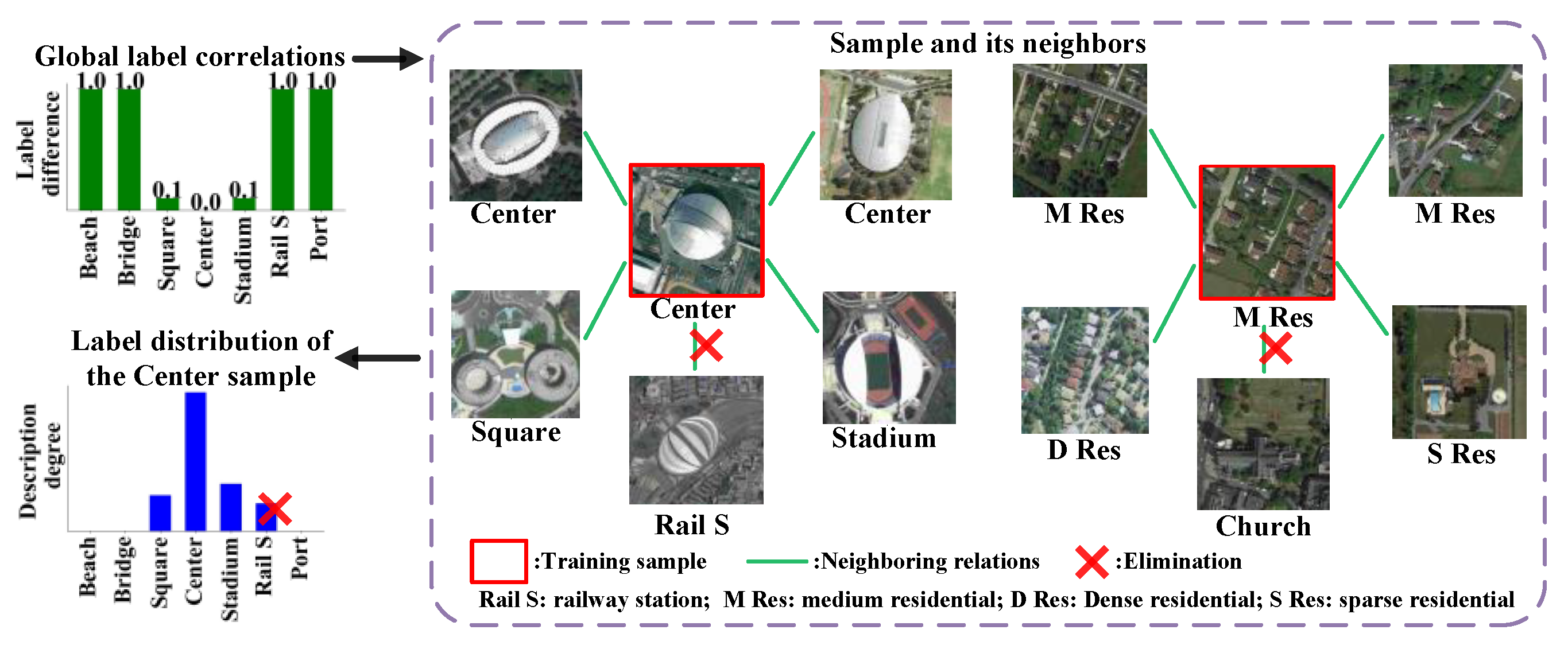
  • We assume that the label ambiguity is caused by sample neighbors having different but correlated labels. As shown in Figure 2, the images of scenes Center, Square, and Stadium share similar visual features; hence, labels Square and Stadium cause the label ambiguity of the Center sample annotated by the red box. As label ambiguity originates from label correlations, we desire to uncover the local sample neighbors that satisfy global label correlations.
  • Subspace learning [12,13,14] has the potential to uncover sample neighbors that satisfy a certain property. To find neighbors having discrimination ability, subspace learning is adopted for semi-supervised learning (SSL) or clustering problems [15,16,17]. In subspace learning, the neighboring relations are formulated as the representation coefficient matrix that takes samples as the dictionary and reconstructs each sample as a linear combination of others, i.e., the self-expressiveness assumption [12]. The sample affinity graph is determined by the coefficient matrix. Discriminative neighbors desire the matrix to be block-diagonal, i.e., neighboring relations occur only between samples of the same label. Many constraints are proposed to purchase the block-diagonal matrix, such as the block-wise [18], low-rank [19], and group-sparse [20] constraints.
  • The subspace learning methods developed for SSL or clustering problems are suboptimal for modeling label ambiguity. The desired discriminative neighbors are used for capturing reliable unlabeled samples in SSL or producing accurate clustering membership. The block-diagonal matrix requires sample neighbors have the same label, which is inappropriate for uncovering the neighbors with different labels.
In this paper, we define a subspace learning problem to model label ambiguity, and the fundamental idea of this paper is shown in Figure 2. First, we predefine the global label correlations, which reflect that Center is similar to Stadium and Square but differs substantially from Rail S. In subspace learning, the objective function penalizes the coefficient matrix using the 1 norm and the label correlations. The 1 norm provides sparse neighbors, such as the Square image and Stadium image, which captures local similarity. According to the label correlations, the neighboring relation between the training sample and the Rail S image is severely penalized, even though the two images are similar. Label propagation among the neighbors leads to the label distribution that can express the label ambiguity of the training sample. The label noise of Rail S is eliminated by using the label correlations. Similarly, the label ambiguity of the M Res sample is caused by the D Res images and S Res images, but not by the Church image, even though the Church image is visually similar to the M Res sample.

1.3. Contributions

In this paper, we uncover the sample neighbors that cause the label ambiguity of aerial images and propose neighbor-based LDL for aerial scene classification, as shown in Figure 3. To be specific, a subspace learning problem is defined to uncover neighboring relations among samples, which includes a 1 norm to capture local sample similarity and a constraint based on global label correlations. During subspace learning, sample neighbors are enforced to share correlated labels. Our method differs substantially from existing methods in two aspects:
  • Different from most subspace learning methods, our method is developed for modeling label ambiguity. Most subspace learning methods emphasize the discrimination ability of neighboring relations, and the learned affinity graph is encouraged to be block-diagonal. Conversely, we aim to uncover neighboring relations among different but correlated labels. Figure 3 shows that our affinity graph is consistent with the global label correlations and is not block-diagonal.
  • Most LDL methods are invalid for generic SLL problems, and we model label ambiguity by jointly capturing local sample similarity and global label correlations. Although the data-dependent LDL (D2LDL) proposed by He et al. [21] has the potential to handle generic SLL problems, it only uses a 1 norm to uncover sample neighbors but overlooks label correlations. In contrast, we introduce label correlations to uncover sample neighbors, which can reduce label noise, as explained in Figure 2.
The main contributions of this paper are two-fold:
  • We define a subspace learning problem, which jointly captures local sample similarity and global label correlations. The neighbor-based label distribution can robustly express label ambiguity.
  • To our knowledge, this is the first LDL work that can manage generic SLL problems. Experiment results demonstrate that using the label distributions can prevent CNNs from over-fitting and assist feature learning.
The remainder of this paper is organized as follows: Section 2 reviews related works, Section 3 formulates the proposed method in detail, Section 4 reports the experimental results, Section 5 presents the discussion, and Section 6 concludes this paper.

2. Related Works

2.1. Deep Learning

Currently, deep learning has been acknowledged as the most successful and widely used approach for aerial scene classification. CNNs are able to produce task-specific deep features that are automatically learned from training sets [1,2], which requires little feature engineering by hand. Thus, the deep features enjoy better representation ability than the low-level features (e.g., local binary patterns) or mid-level features (e.g., bag of features). How to further improve the deep features remains a hot research topic [22,23,24,25]. Recently, the attention mechanism has been introduced into network structures to learn more discriminative features, such as the spatial attention [24] for capturing class-specific regions, or the channel attention [25] for selection of important features. As the deep features are usually redundant, some methods adopt meta-heuristic algorithms [26] to select the most effective features among the high-dimensional features [27,28], which leads to compact and robust features.
Overall, many studies related to deep learning focus on network structures or feature selection; however, there are limited works concerning label representations. In this paper, we build a label representation based on label distributions, which is used to guide the feature learning during network training.

2.2. Label Distribution Learning (LDL)

As an extension of MLL [3,4,5], LDL [6,7] is a paradigm for handling label ambiguity. Studies on LDL include two aspects: the former is to learn accurate classifiers [29,30,31], and the latter is to build label distributions that can express label ambiguity. The goal of this paper is to construct label distributions for aerial images. The strategies for constructing the distributions can be summarized as three types:
The first type is the Gaussian-based label distribution [7], as shown in Figure 1. The Gaussian distribution has established its effectiveness in the fields of age estimation [8], pose estimation [10], and crowd counting [11]. The problem of age estimation can be cast as a classification problem by viewing each age as a label. The classification performance can be improved by using the Gaussian distribution for CNN training. Similarly, using the Gaussian distribution yields satisfactory performance for pose estimation and crowd counting.
The second type is incomplete label distribution learning (IncomLDL) [32], which aims to recover missing labels from partially labeled samples provided by humans. IncomLDL methods [32,33,34,35] usually regularize the label distribution matrix of all samples by a manifold constraint and a low-rank constraint. The former captures local similarity [33]. The latter models the label correlations that exist in the partially labeled samples (e.g., label co-occurrence), which force the completed matrix to agree with the existed label correlations [32]. However, IncomLDL methods are invalid for generic SLL problems due to the lack of label correlations that can guide the construction of label distributions.
The third type is the adaptive label distribution [21,36,37,38] which aims to enhance the adaption to data variations. Among the methods for adaptive label distributions, the data-dependent LDL (D2LDL) [21] has the potential to be transformed into scene classification problems, which models label ambiguity regarding human age though sample neighbors and the label distributions are computed as label propagation. D2LDL adopts subspace learning to compute the sample affinity graph and the coefficient matrix is constrained by the 1 norm to obtain sparse neighbors. Compared to the Gaussian distribution, D2LDL is more flexible for data variations. However, D2LDL only captures local similarity through the 1 norm but overlooks label correlations, which may cause neighbors conflicting with label correlations and thus produce label noise, as explained in Figure 2.

2.3. Subspace Learning

Subspace learning [12,13] has gained success in semi-supervised learning and clustering problems [15,16,17,18,19]. The affinity graph produced by subspace learning can provide the graph Laplacian matrix for semi-supervised learning [17], and also can be used for spectral clustering [15]. The self-expressiveness assumption [12] states that each sample can be represented as a linear combination of other samples. Thus, samples are embedded into many local subspaces expressed by the representation coefficient matrix. Samples that lie in the same subspace are neighboring. Formally, denote the sample features and coefficient matrix as X and Z respectively, where X R D × N , Z R N × N , and D, N represent the feature dimension and sample number, respectively. Sparse subspace clustering (SSC) [12] is a typical subspace learning approach, which is formulated as:
m i n Z , E Z 1 + λ e E 1         s . t .         X = X Z + E ,       d i a g ( Z ) = 0
where the 1 norm · 1 guarantees sparsity [39], and λ e is a trade-off parameter. The representation error E is incorporated to resist outliers, where E R D × N . The operator diag ( · ) indicates constructing diagonal matrices. The constraint diag ( Z ) = 0 prevents Z from being an identity matrix. A non-zero coefficient Z ( m , n ) indicates that samples m and n lie in the same subspace and the two samples are neighboring. To ensure that the neighboring relations are non-negative and symmetric, the affinity graph A is defined as:
A = 1 2 ( | Z | + | Z T | )
SSC can uncover adaptive and sparse neighbors and is robust to outliers. Thus, SSC and its variants [40,41,42,43] have realized impressive clustering performance. In SSL or clustering problems, the desirable neighbor assignment is that the affinity graph has exact C connected components (i.e., block-diagonal structure), where C is the class number. Various constraints have been imposed on the coefficient matrix to encourage the block-diagonal structure [15,16,17,18,19,40,41,42,43].
Compared to D2LDL, our method jointly considers sparsity and label correlations. Different from the subspace learning for SLL or clustering problems, we aim at modeling label ambiguity and do not purchase the block-diagonal structure.

3. Proposed Method

We define a subspace learning problem to model the label ambiguity of aerial images. As shown in Figure 3, the constructed label distributions are used for CNN training. At the testing stage, predictions are determined by the fully connected (FC) layer that is connected to the single truth label.
Notations: The matrices in this paper are denoted in boldface. For a matrix M, its entry ( i , j ) and the jth column are denoted as M ( i , j ) and M ( · , j ) , respectively. The 1 norm and Frobenius norm are denoted as · 1 and · F , respectively. 0, 1, and I represent a vector of 0s, a vector of 1s, and an identity matrix, respectively. The symbol descriptions are listed in Table 1.

3.1. Modeling Label Ambiguity

Label ambiguity originates from the visually similar samples that have different but correlated labels. As shown in Figure 2, the label ambiguity of the training sample is caused by the similar images of Square and Stadium. In Figure 2, although the Rail S image is similar to the training sample, it is unreasonable to assume label ambiguity between the training sample and the Rail S image because scenes Center and Rail S are substantially different in terms of the global label correlations. According to the definition of LDL [6,7], label ambiguity should agree with label correlations. As shown in Figure 1, the Gaussian distribution only includes the labels that are near the sample ground truth. In the methods of IncomLDL [32], the label distribution matrix is regularized by a low-rank constraint to capture label correlations, which force the completed matrix to accord with the label correlations.
Our goal is to uncover the sample neighbors that cause label ambiguity. As explained by SSC [12], a non-zero coefficient Z ( m , n ) indicates that samples m and n are neighboring. To model label ambiguity, ideal neighboring relations should meet the following properties:
  • The agreement with local sample similarity. If samples m and n have similar features, samples m and n are neighboring, i.e., Z ( m , n ) 0 .
  • The consistence with global label correlations. If samples m and n have substantially different labels, samples m and n are not neighboring, i.e., Z ( m , n ) = 0 .

3.1.1. Uncovering Sample Neighbors

We define a subspace learning problem to uncover the ideal neighboring relations. Firstly, a global label correlation matrix G is predefined to formulate label differences, where G R + C × C . Element G ( i , j ) is specified as a large value if labels i and j are importantly different, and G ( i , j ) is small if labels i and j are correlated. By introducing G into objective Function (1), the subspace learning problem is formulated as follows:
m i n Z , E Z 1 + α z m , n G ( y m , y n ) | Z ( m , n ) | + λ e E 1           s . t .         X = X Z + E ,         d i a g ( Z ) = 0
where α z is a trade-off parameter and we set it as 1.0. On the one hand, if sample features X ( · , m ) and X ( · , n ) are similar, Z ( m , n ) is large because each sample tends to select similar samples to reconstruct itself. On the other hand, if samples m and n have substantially different labels, the large element G ( y m , y n ) enforces Z ( m , n ) = 0 and thus the neighboring relation between samples m and n is prohibited. Hence, the objective Function (3) can uncover ideal neighboring relations that jointly capture local similarity and label correlations. Note that D2LDL [21] adopts standard SSC (i.e., the objective Function (1)) to compute neighboring relations, which overlooks label correlations.

3.1.2. Predefining Label Correlations

The global label correlations G should be properly predefined. A simple yet effective approach for evaluating label correlations is to utilize additional knowledge from confusion matrices [44,45]. Following this approach, we use the Library for support vector machines (LIBSVM) [46] to train classifiers on training sets, and compute confusion matrices on validation sets. We use pretrained CNNs as feature extractors, in which the activations of the penultimate FC layer serve as image features.
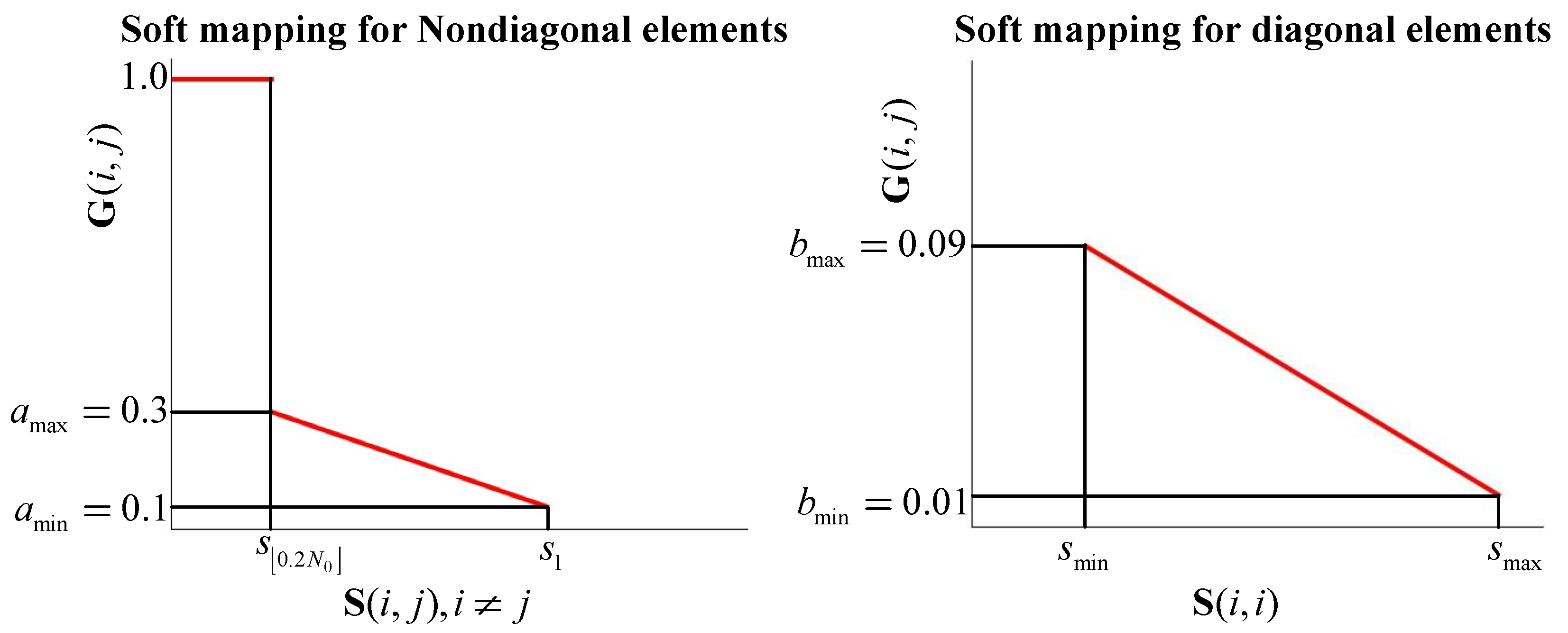
Denote the confusion matrix as H R C × C , where element H ( i , j ) denotes the rate at which samples of label i are classified as label j. According to Wang et al. [44], the symmetric similarity matrix S R C × C is computed as S = 1 / 2 ( H + H T ) . A large S ( i , j ) implies a similar label pair ( i , j ) . In this paper, label pairs ( i , j ) that are in the top 20% in terms of similarity are regarded as correlated labels. Specifically, we sort all the non-diagonal elements { S ( i , j ) } i j of S as a descending sequence and delete the repeated values from the sequence. This leads to a sequence ( s 1 , s 2 , , s N 0 ) , in which s 1 implies the most similar label pair. Labels i and j are thought of as correlated if S ( i , j ) s 0.2 N 0 , where the function · denotes the rounding down operator. Denote the maximal and minimal values in the classification accuracies { S ( i , i ) } i = 1 ~ C as s max and s min , respectively. Since the role of G is to express label differences, G ( i , j ) should be inversely proportional to S ( i , j ) . Soft mappings are defined to compute G, as illustrated in Figure 4. Elements of G are computed as follows:
G ( i , j ) = { 1 if   S ( i , j ) < s 0.2 N 0   and   i j s 1 S ( i , j ) s 1 s 0.2 N 0 ( a max a min ) + a min if   S ( i , j ) s 0.2 N 0   and   i j s max S ( i , i ) s max s min ( b max b min ) + b min if   i = j
where the hyper-parameters a min , a max , b min , and b max are set to 0.1, 0.3, 0.01, and 0.09, respectively. On the one hand, label differences for correlated label pairs range from a min to a max , and a high S ( i , j ) leads to a small G ( i , j ) . On the other hand, a low classification accuracy S ( i , i ) causes a relatively large G ( i , j ) , as the samples of label i tend to be scattered.

3.1.3. Optimization

We optimize the objective Function (3) by resorting to the alternating direction method of multipliers (ADMM) [47]. First, we replace G with another correlation matrix Θ R N × N , the elements of which are Θ ( m , n ) = G ( y m , y n ) . Θ ( m , n ) is large when samples m and n have substantially different labels. In addition, an auxiliary matrix J R N × N is introduced. Considering Θ and J, objective (3) equals:
min Z , J , E Z 1 + α z Θ Z 1 + λ e E 1 = min Z , J , E ( 1 1 T + α z Θ ) Z 1 + λ e E 1               s . t .         X = X J + E ,       J = Z diag ( Z )
where operator is the elementwise product. Using ADMM, the augmented Lagrange function of objective (5) is
( Z , J , E , Y 1 , Y 2 ) = ( 1 1 T + α z Θ ) Z 1 + λ e E 1 + tr [ B 1 T ( X X J E ) ] + tr [ B 2 T ( J Z + diag ( Z ) ) ] + μ 2 ( X X J E F 2 + J Z + diag ( Z ) F 2 )
where B 1 and B 2 are Lagrange multipliers and μ is a penalty parameter. Since ( · ) is separable, we can alternatively update Z, J, E, B 1 , and B 2 , while fixing others.
Update of Z:
We update Z by solving the following problem:
Z t + 1 = arg min Z     1 μ t ( 11 T + α z Θ ) Z 1 + 1 2 Z + diag ( Z ) U t F 2
where t denotes the tth iteration and U t = J t + 1 / μ t B 2 , t . The closed-form solution of Z is
Z t + 1 = Z ˜ t + 1 d i a g ( Z ˜ t + 1 )
The elements of Z ˜ can be obtained by applying the soft-thresholding operator [47]:
Z ˜ t + 1 ( m , n ) = sgn ( U t ( m , n ) ) max ( | U t ( m , n ) | 1 + α z Θ ( m , n ) μ t , 0 )
Solution (8) shows that a large Θ ( m , n ) encourages Z ˜ t + 1 ( m , n ) = 0 , which eliminates the neighboring relations between two substantially different labels y m and y n . Thus, the uncovered neighboring relations are consistent with label correlations.
Update of J:
Fixing other variables, the problem for J becomes:
J t + 1 = arg min J tr [ B 1 T ( X X J E ) ] + tr [ B 2 T ( J Z + diag ( Z ) ) ] + μ 2 ( X X J E F 2 + J Z + diag ( Z ) F 2 )
Let the derivative with respect to J be zero, then the solution is expressed as
J t + 1 = ( X T X + I ) 1 [ X T ( X E t + 1 μ t B 1 , t ) + Z t diag ( Z t ) 1 μ t B 2 , t ]
Update of E:
While other variables are fixed, we update E as follows:
E t + 1 = arg min E   λ e μ t E 1 + 1 2 E V t F 2
where V t = X X J t + 1 + 1 / μ t B 1 , t . E can be obtained by applying the soft-thresholding operator [47]:
E t + 1 ( m , n ) = sgn ( V t ( m , n ) ) max ( | V t ( m , n ) | λ e μ t , 0 )
Update of B 1 and B 2 :
The Lagrange multipliers can be updated by using the gradient ascent procedure:
B 1 , t + 1 = B 1 , t + μ t ( X X J t + 1 E t + 1 ) B 2 , t + 1 = B 2 , t + μ t ( J t + 1 Z t + 1 + diag ( Z t + 1 ) )
For clarity, the ADMM algorithm for solving objective (3) is outlined in Algorithm 1.
Algorithm 1: Solving the objective Function (3) through ADMM
Input: X, Θ , α z , λ e , μ 0
Initialize: Z = J = 0 , B 1 = 0 , B 2 = 0 , t = 0 , t max = 30 , μ max = 10 10 , ρ = 1.1 , ε = 10 4
Compute the constant term ( X T X + I ) 1 in Equation (9)
While the convergence conditions are not satisfied:
 1: update Z t + 1 according to Equations (7) and (8)
 2: update J t + 1 according to Equation (9)
 3: update E t + 1 according to Equation (10)
 4: update B 1 , t + 1 and B 2 , t + 1 according to Equation (11)
 5: update μ t by μ t + 1 = min ( μ max , ρ μ t )
 6: check the convergence conditions:
     X X J t + 1 E t + 1 < ε and J t + 1 Z t + 1 + d i a g ( Z t + 1 ) < ε
 7: t = t + 1
 8: if t > t max , break
End while
Output: Z t + 1

3.2. Constructing Label Distributions

3.2.1. Label Propagation

Label ambiguity can be modeled through the affinity graph A and we construct label distributions through label propagation. Denote the matrix of sample ground truth as Y, where Y R C × N with Y ( i , n ) = 1 if i = y n , and Y ( i , n ) = 0 otherwise. Denote the label distributions of all samples as P, where P R C × N . Y ( · , n ) and P ( · , n ) represent the ground truth and label distribution of the nth sample, respectively. According to Equation (2), the affinity graph can be determined by the coefficient matrix, i.e., A = 1 / 2 ( | Z | + | Z T | ) . The label distribution P ( · , n ) can be computed as the following label propagation:
P ( · , n ) = 1 d n ( Y ( · , 1 ) A ( 1 , n ) + Y ( · , m ) A ( m , n ) + Y ( · , N ) A ( N , n ) ) = Y ( A ( · , n ) d n ) ,   d n = m = 1 N A ( m , n )
where d n is the degree [15] of sample n and the term A ( · , n ) / d n represents the transition probabilities [48]. d n acts as the normalization term to ensure that i = 1 C P ( i , n ) = 1 .
Equation (12) shows that if sample m is the neighbor of sample n, a positive A ( m , n ) incorporates the label of sample m into the label distribution of sample n; if two samples are not neighboring, A ( m , n ) = 0 , and the label of sample m has no influence on P ( · , n ) . Thus, sample n is associated with its neighbor labels and thus P ( · , n ) describes the label ambiguity regarding sample n.

3.2.2. Rectifying Label Distributions

We use the label distribution for CNN training and thus the sample ground truth should account for the highest intensity in the distribution. Since the images of the same class usually share similar features, the majority of sample neighbors have the same label to the sample ground truth. In most label distributions, the ground truth has the highest intensity. However, the adaptively uncovered neighbors cannot ensure that the ground truth always occupies the highest intensity in all label distributions. Referring to D2LDL that use the ground truth to rectify label distributions [21], we compute the rectified distributions P r as follows:
P r = 0.5 P + 0.5 Y
where term 0.5 Y ensures that y n has the highest intensity in P r ( · , n ) . We use P r for CNN learning.

3.3. CNN Learning Framework

The label distributions are used as label-level regularization in network learning. The network jointly learns the task of scene classification and the task of learning label distributions P r . The multitask loss is defined as
L = L c l s ( , Y ) + λ l L l d l ( , P r )
where represents the set of training images and λ l is a trade-off parameter. We set λ l to 0.5. Term L c l s ( · ) adopts the common softmax loss and term L l d l ( · ) uses Kullback–Leibler (KL) loss, respectively. The KL divergence is defined as:
KL ( P r ( · , n ) , P ^ ( · , n ) ) = i = 1 C P r ( i , n ) ln P r ( i , n ) P ^ ( i , n ) i = 1 C P r ( i , n ) ln P ^ ( i , n )
where P ^ ( · , n ) is the network output generated by a softmax function. Hence, L l d l ( · ) is computed as follows:
L l d l ( , P r ) = 1 N n = 1 N i = 1 C P r ( i , n ) ln P ^ ( i , n )
The learning framework is supervised not only by sample ground truth but also the side information about the label ambiguity of samples. Compared to the ground truth, the label distributions are more informative since it incorporates correlated labels. As mentioned in previous studies [7,9,10,49], informative label representations enable CNNs to learn robust features. Additionally, the label distribution is label smoothing in terms of label ambiguity. As explained in References [49,50,51,52], label smoothing can prevent networks from over-fitting.

4. Experiments and Results

To examine the role of modeling label ambiguity, the proposed method is applied to two CNN backbones, namely VGGNet (VGG) and ResNet, and we conduct experiments on two aerial scene datasets: the aerial image dataset (AID) [1] and NWPU_RESISC45 (NR) [2]. As shown in Figure 5, the two datasets are challenging due to the large intraclass variations and small interclass distinctions.

4.1. Implementation Details

4.1.1. Datasets and Protocols

The AID dataset [1] is comprised of 10,000 600 × 600 images, which cover 30 scene classes. Following previous studies in which AID was used [1,53,54,55,56], we adopt the data division strategy of AID-0.2, where the training/validation/testing ratio is 0.2/0.2/0.6. The NR dataset [2] includes 45 scene classes, each with 700 256 × 256 images. Similar to previous studies [2,22,23,55,56,57,58,59], data division strategy NR-0.1 is used: the training/validation/testing ratio is 0.1/0.1/0.8. Note that the relatively low training ratios (i.e., the 0.2 on AID and 0.1 on NR) are adopted to study the effect of label distributions in improving data utilization. Moreover, we apply no data augmentation strategy, except that there is extra specification.
Following the common evaluation protocol of aerial scene classification [1,2], we train networks under the designated training ratios, and report the overall accuracy (OA) on testing sets. To obtain stable results, we report the average accuracies over 5 trials. For preprocessing, we resize all images to 224 × 224, subtract the mean from the resized images, and divide them by the standard deviation for each color channel.

4.1.2. Network Backbones

The popular VGGNet and ResNet have demonstrated promising performance for aerial scene classification. We separately utilize VGG-16bn [60] and ResNet50 [61] as the backbones of our networks. The networks are initialized as the weights that were pretrained on ImageNet, and the weights are optimized using stochastic gradient descent. The learning rate, momentum, and weight decay are set to 0.001, 0.9, and 0.0005, respectively. Each network is trained for 50 epochs using minibatches of 16. During training, the learning rate is reduced to one tenth when the loss values stop decreasing.

4.1.3. Parameters for Subspace Learning

In the objective Function (3), the feature matrix X is extracted from the penultimate FC layer of pretrained networks (VGG or ResNet) and we reduce the feature dimension, D, to 100 through principal component analysis (PCA). As recommended by Elhamifar et al. [12], λ e is calculated as β / min n   max m n X ( · , m ) 1 , where β is set to 20, as in Reference [15]. The parameter μ 0 in the ADMM algorithm is set to β . For a fair comparison, λ e and the ADMM parameters are kept the same for both D2LDL and our method.
All the algorithms are developed in Python under the PyTorch framework. The experiments are implemented on a workstation with an I7-8700K CPU and a Titan XP GPU.

4.2. Analysis of Label Distributions

To explore the uncovered sample neighbors and the constructed label distributions, we implement experiments on the AID-0.2 dataset using VGG pretrained features. To intuitively illustrate the results of label propagation, we display the label distributions P but not the rectified distributions P r .

4.2.1. Agreement with Local Similarity

The images of the same scene may exhibit different label distribution patterns due to the large intraclass variations. Within the same class, similar images should share close distribution patterns. To observe the distribution patterns, we group the label distributions of the same class into 3 clusters by K-means, as shown in Figure 6.
The local similarity among the cluster 3 images reflects that these images share similar building appearance with the Indus images. Accordingly, the label distributions in cluster 3 specify relatively high intensities on the Indus label, which agrees with the local similarity. The explanation is that the sample tends to select similar neighbors to reconstruct itself during subspace learning, and thus the images in cluster 3 have many Indus neighbors. Analogously, the local similarity among the cluster 1 shows that the images contain obvious railway station buildings, and thus the distributions in cluster 1 are dominated by the Rail S label.
Therefore, the label distributions agree with local similarity, and can adapt to the intraclass variations. Additionally, our distributions also support the conclusions of recent studies [21,36,37,38,62,63]: label distributions should vary with data variations.

4.2.2. Consistence with Label Correlations

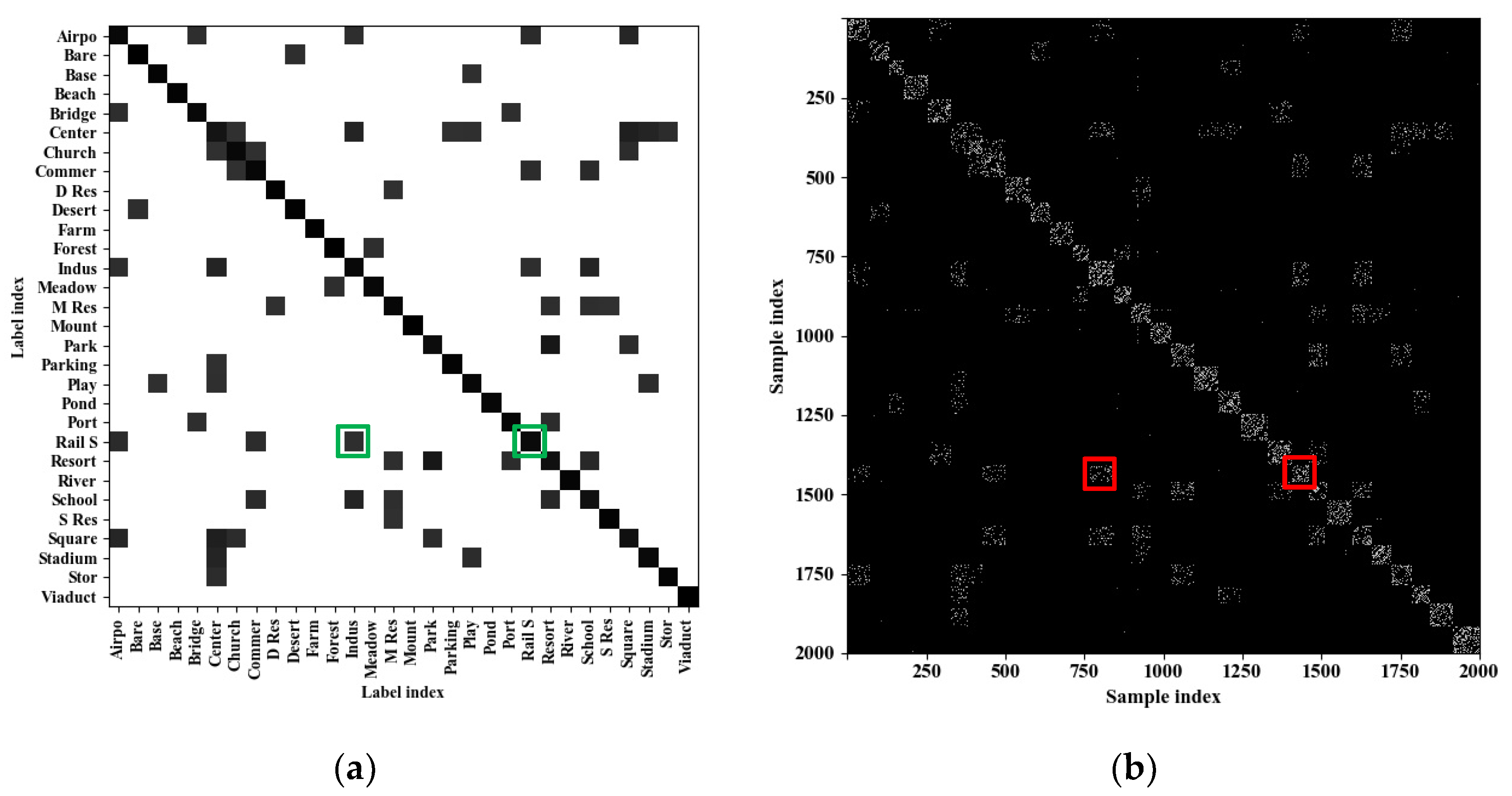
Neighboring relations that cause label ambiguity should be consistent with label correlations. Figure 7 shows the global label correlations G evaluated on the confusion matrices, and the affinity graph A determined by the coefficient matrix Z. We have the following 3 observations.
  • The dark elements in G indicate the correlated label pairs. For example, the green boxes show that scenes Rail S and Indus are correlated. The explanation is that lots of Rail S images and Indus images are confused with each other in validation sets.
  • The light elements in A are globally consistent with the dark elements in G. For example, the red boxes suggest that many Rail S samples have Indus neighbors. The explanation is that Z is penalized by G in objective Function (3) and thus the neighboring relations are consistent with label correlations.
  • A is not block-diagonal, in which there are neighboring relations among samples of different labels. In contrast, the affinity graph for SSL or clustering problems [15,16,17,18,19,40,41,42,43] are encouraged to be block-diagonal so as to yield discriminative neighbors.

4.2.3. Comparisons with D2LDL

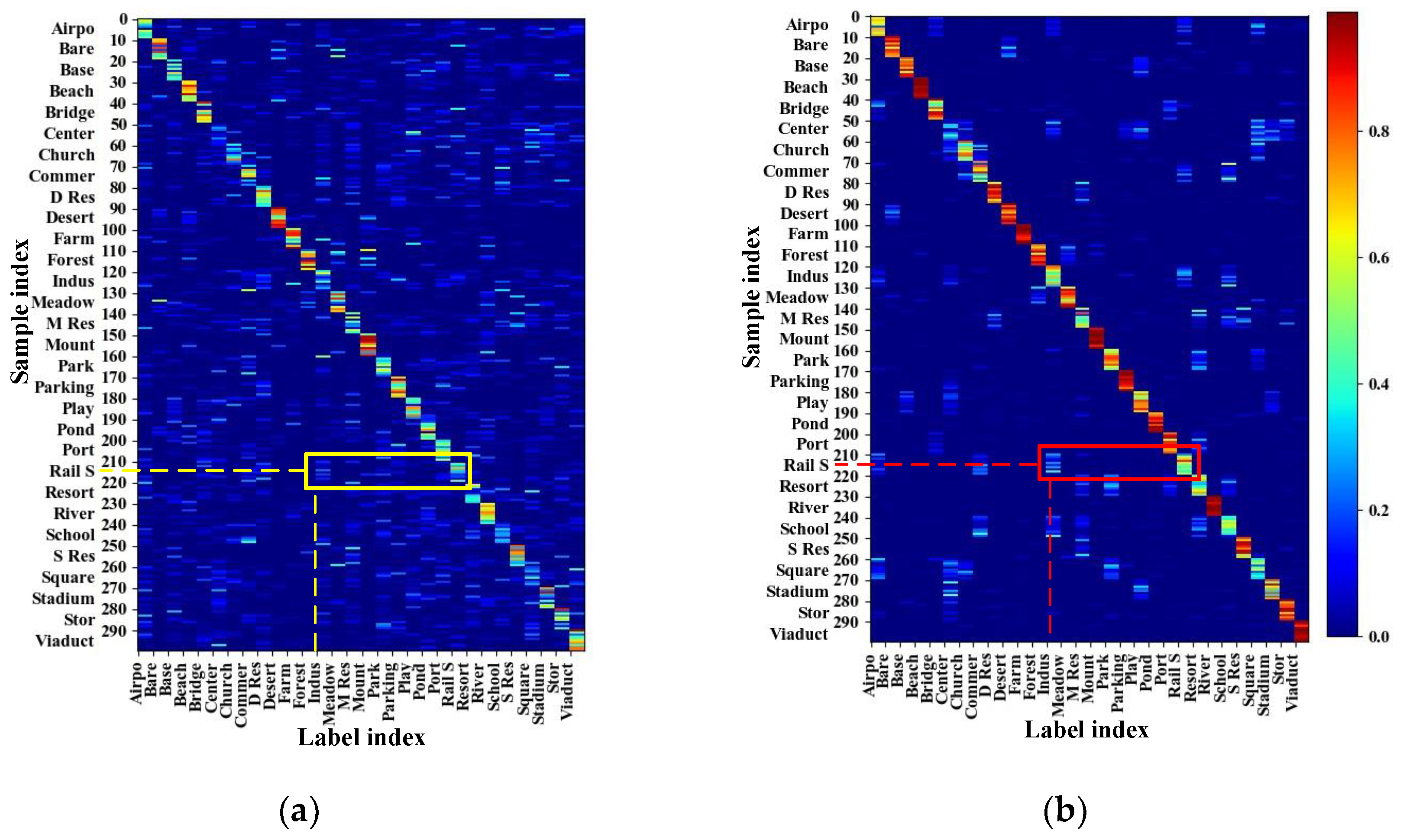
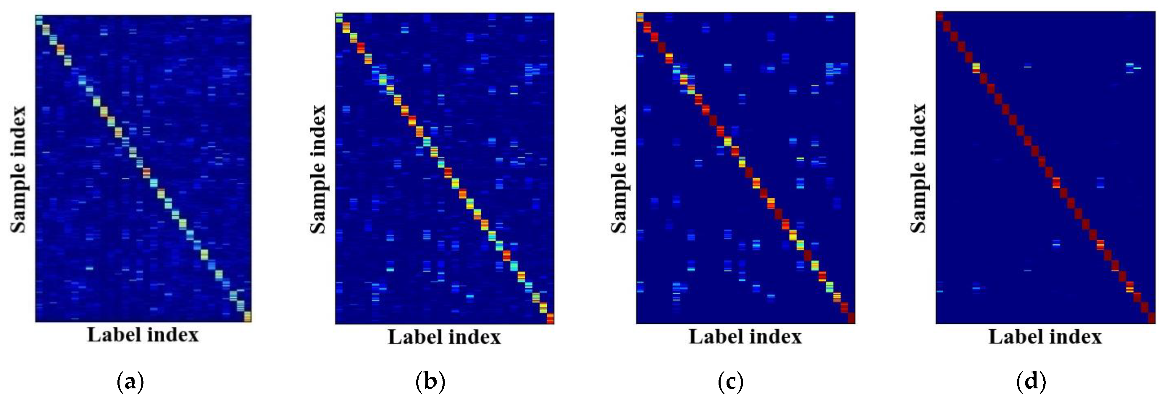
D2LDL [21] exploits the 1 norm to uncover sample neighbors but overlooks label correlations, which may cause label noise. The label noise reflects unreasonable neighbors, such as the Rail S image in Figure 2. Serious noise may cause the distorted distributions, in which the sample ground truth fails to account for the highest intensity. We refer to the distribution P ( · , n ) as a distorted distribution if P ( y n , n ) P ( i y n , n ) . Figure 8 shows the label distributions produced by D2LDL and our method, and N d is the number of distorted distributions which can be thought of as the measurement of noise level. We have the following 3 observations:
  • D2LDL can construct adaptive label distributions but results in many distorted distributions, which imply gross label noise. For example, the yellow rectangle shows that many Rail S samples are associated with label Indus, which reflects the correlation between Rail S and Indus.
  • Our method produces much less distorted distributions compared to D2LDL (138 vs. 411), which suggests the reduction of noise. Compared to the yellow rectangular region, the red rectangular region is ‘cleaner’, which indicates that fewer samples are contaminated by noisy labels. Therefore, label noise can be reduced by introducing label correlations to regularize the discovery of neighbors.
  • The distorted distributions of our method originate from severely confused image contents. As shown in Figure 9, the image semantics are confused with the ambiguous labels even by humans.

4.3. Analysis of the Network Performance

In this section, we explore the proposed method from the perspective of classification performance and learned features.

4.3.1. Classification Accuracy

The label distributions are used as label representations for CNN training and we adopt five methods to construct label representations, as described in Table 2.
Across experiments, our label distributions are replaced by the label representations that are produced by the competing approaches, and other parts of the CNN learning framework remain unchanged. The classification accuracies of the testing sets on AID-0.2 and NR-0.1 are listed in Table 3.
The comparisons demonstrate the advantages of our method over the competing approaches, regardless of the dataset or network backbone. We observe the following:
  • LSR, CWL, and D2LDL all realize higher accuracies than using sample ground truth; hence, the efforts to address label ambiguity are beneficial for aerial scene classification.
  • CWL methods yield competitive performance over D2LDL, which demonstrates the role of incorporating label correlations into label representations.
  • Our methods clearly outperform CWL. The reason is that the label representations of CWL are class-specific and thus are inflexible to adapt to the large intraclass variation of scene images. In contrast, our neighbor-based label distributions capture local sample similarity and can express different patterns of label distributions.
  • Our methods substantially outperform D2LDL, which highlights the effectiveness of considering label correlations. Figure 10 presents the comparisons in terms of confusion matrices. There are large accuracy gaps in the scenes of Center (0.81 vs. 0.78), Rail S (0.91 vs. 0.84), and School (0.74 vs. 0.69). These scenes are usually comprised of complicated visual contents and are prone to the involvement of diverse scene labels. Accordingly, these scenes are susceptible to label noise. Facilitated by label correlations, our methods reduce the label noise and can robustly encode label ambiguity. Therefore, our label distribution is effective in representing complex scenes.

4.3.2. Feature Robustness

The label distributions are more informative compared to sample ground truth and can enhance feature robustness. We select the outputs of the fc7 layer in the VGG backbone as image features, and the corresponding two-dimensional representations generated by the t-Distributed Stochastic Neighbor Embedding (t-SNE) [64] are plotted in Figure 11. We observe that features produced by N-LDL-v are more compact than those produced by original VGG, such as the features of scenes Airport (Airpo), Park, and Port. This compactness suggests that feature robustness is improved by using the informative label distributions.

4.4. Comparisons with State-of-the-Art Methods

Our method is compared with previous methods for aerial scene classification, which are listed in Table 4 and have been validated on AID-0.2 and NR-0.1 in the original literatures. We have following observations:
  • Although we only use common network structures (i.e., ResNet), our method achieves comparable performance compared to recent deep learning methods which devise complicated network structures, such as Attention-GAN [22] and CapsNet [56]. The explanation is that the label distributions substantially improve data utilization by associating samples with multiple labels. Thus, our method is a simple yet effective approach for aerial scene classification.
  • SF-CNN [57] slightly surpasses our method on NR-0.1 (89.89 vs. 89.80). The SF-CNN, namely scale-free CNN, enlarges sample number by 4 times through resizing each image to 4 scales from 224×224 to 400 × 400. In contrast, our computational complexity is much lower because we do not apply data augmentation.

4.5. Experiments Using Different Sizes of Datasets

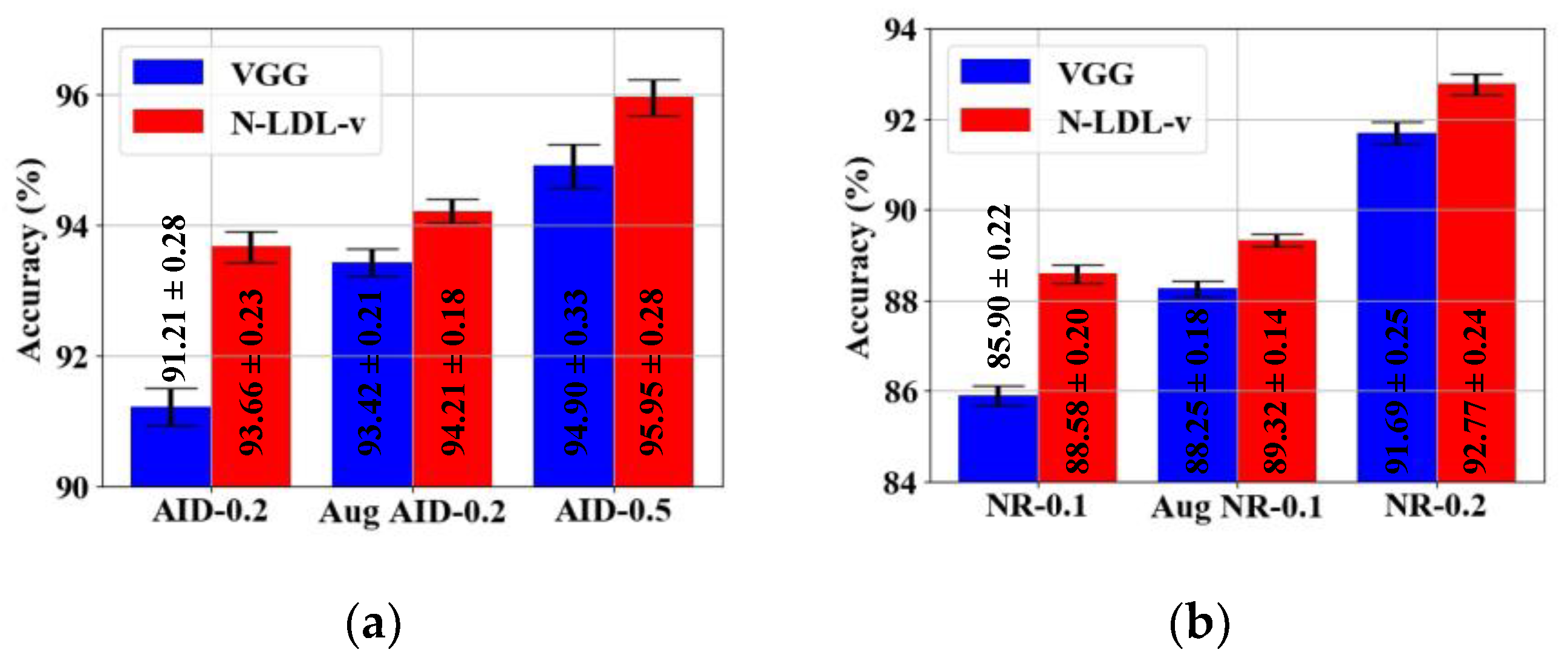
Our method achieves satisfying performance on small datasets (i.e., AID-0.2 and NR-0.1), and we further study our method on relatively large datasets by using data augmentation and relatively large training ratios. For data augmentation, training images are randomly cropped at 50% of the original image coverage. The cropped and original images are flipped horizontally or vertically. Thus, the sizes of training sets are enlarged by 4 times. Label distributions of the augmented images are also constructed through subspace learning. The augmented training sets for AID-0.2 and NR-0.1 are denoted as Aug AID-0.2 and Aug NR-0.1, respectively. On the other hand, we increase the training ratios for datasets AID and NR to 0.5 and 0.2, forming the data divisions of AID-0.5 and NR-0.2, respectively. The validation ratios remain unchanged, and the rest of the images serve as testing sets. Both the AID-0.5 and NR-0.2 are also commonly used data divisions [53,54,55,56,57]. Original VGG is selected as the baseline. Using different sizes of training sets, Figure 12 plots the learning curves and Figure 13 presents the classification results. We have the following observations:
(1) Our method can mitigate over-fitting problems.
Using different sizes of training sets, Figure 12 shows that the original VGG always yields saturated training accuracy, nearly 100%, which indicates over-fitting problems. However, N-LDL produces lower training accuracy but higher validation accuracy, and the gap between training accuracy and validation accuracy becomes smaller, which suggests less over-fitting and better generalization.
As mentioned by Szegedyet al. [50] and Pereyra et al. [51], despite using large datasets, networks are still prone to over-fitting due to networks learning to assign full probability to sample ground truth and thus outputting too-confident predictions. Some studies [50,51,62] demonstrate that label smoothing can alleviate over-fitting by maintaining reasonable ratios between the logits of the correct and incorrect classes. The label distributions are label smoothing in terms of label ambiguity. N-LDL enables networks to assign probability to correlated labels, which helps to improve generalization.
(2) Our method is effective especially for small datasets.
Figure 13 demonstrates that the accuracy improvements brought about by our method on the small datasets (e.g., AID-0.2) are more significant than that on the relatively large datasets (e.g., Aug AID-0.2 and AID-0.5). When the original VGG is trained with the small datasets, over-fitting problems seriously degrade the generation ability of learned features. By alleviating over-fitting, N-LDL-v significantly improves classification performance on the small datasets. Although there are over-fitting symptoms on the large datasets, networks learn to fit more training samples, which enable learned features to be adaptive and reduce the damage caused by over-fitting. As a result, the improvements brought by N-LDL on the large datasets are degraded.
Our label distributions are used for regularizing output distributions of networks, which can improve generalization. As explained by some studies [65,66] that also work to regularize the output distributions, the attempts to improve generalization are effective especially in the case that the amount of training data is limited. Therefore, the benefit of our method is more significant for small datasets.

4.6. Influence of Parameters and Time Efficiency

In this subsection, we discuss the influence of parameters and the time efficiency of the proposed method. The experiments are conducted using VGG pretrained features.

4.6.1. Influence of α z

α z controls the importance of the global label correlations in the objective Function (3). Figure 14 presents the resulting label distributions of different α z on the AID-0.2 dataset. Similar to Figure 8, we display 10 label distributions for each class on AID-0.2 since the training samples are too numerous to be fully presented. A too small α z (e.g., 0.1) causes substantial noise as the effect of label correlations is weak. Conversely, setting α z too large (e.g., 10) severely reduces the intensities of the correlated labels, which degrades the ability to express label ambiguity. Therefore, we fixed α z as 1.0 in our method.

4.6.2. Influence of D

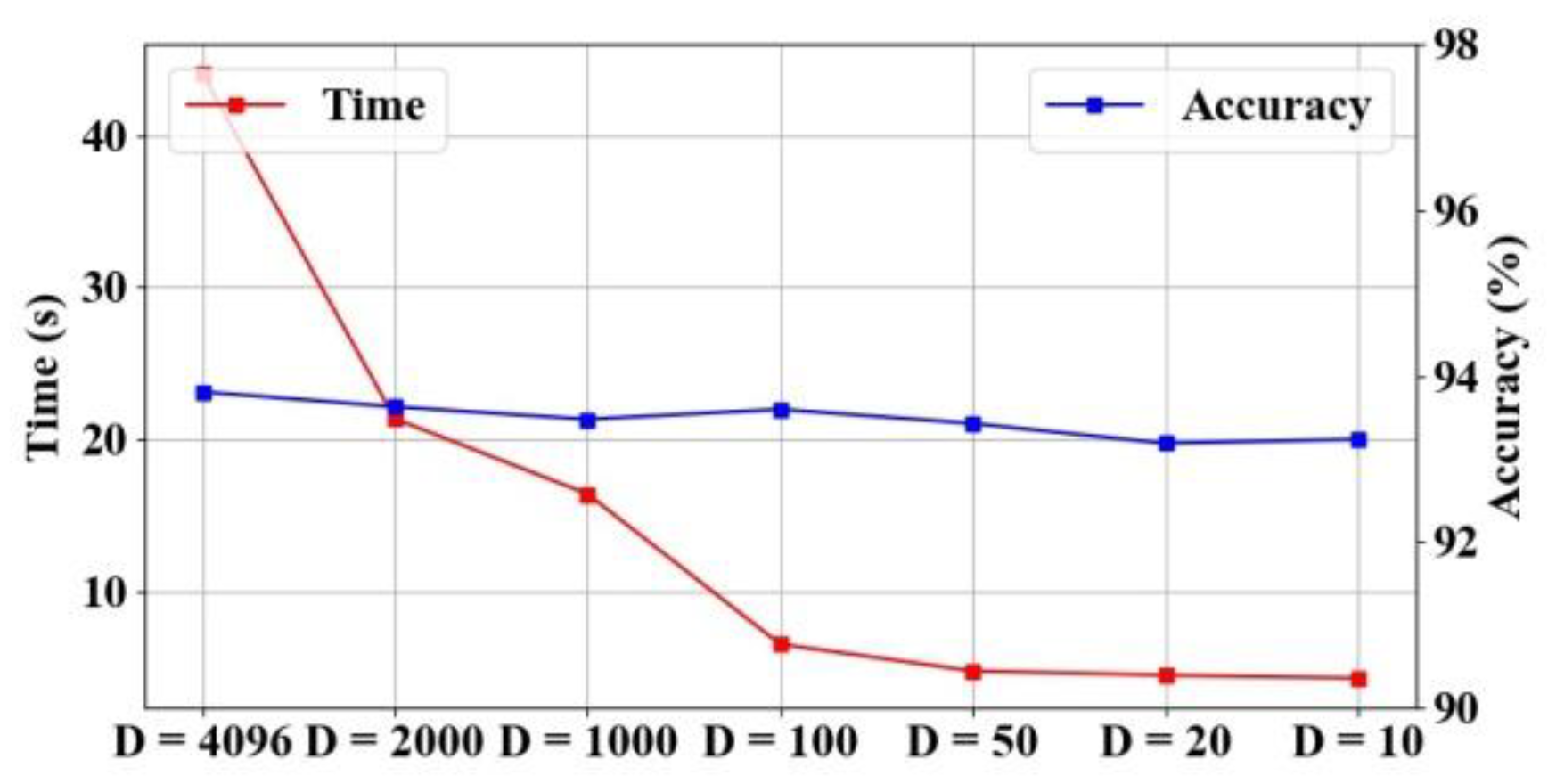
We use pretrained CNN features for subspace learning. To accelerate subspace learning, we reduce feature dimensions, D, via PCA. Figure 15 plots the influence of different feature dimensions, D. On the one hand, the low feature dimensions substantially reduce the time consumption for optimizing Equation (3). On the other hand, when D 50 , the decrease of D has little influence on classification accuracies. The explanation is that original CNN features are high-dimensional and redundant, and reducing the feature dimensions via PCA still preserves the most image information. Thus, features transformed by PCA can also deliver major image contents and are valid for uncovering sample neighbors. However, using too small D (e.g., 10) is insufficient to fully represent image semantics, which is harmful for constructing proper label distributions and thus degrades the classification performance. To balance the time consumption and representation ability, we set D to 100.

4.6.3. Influence of λ l

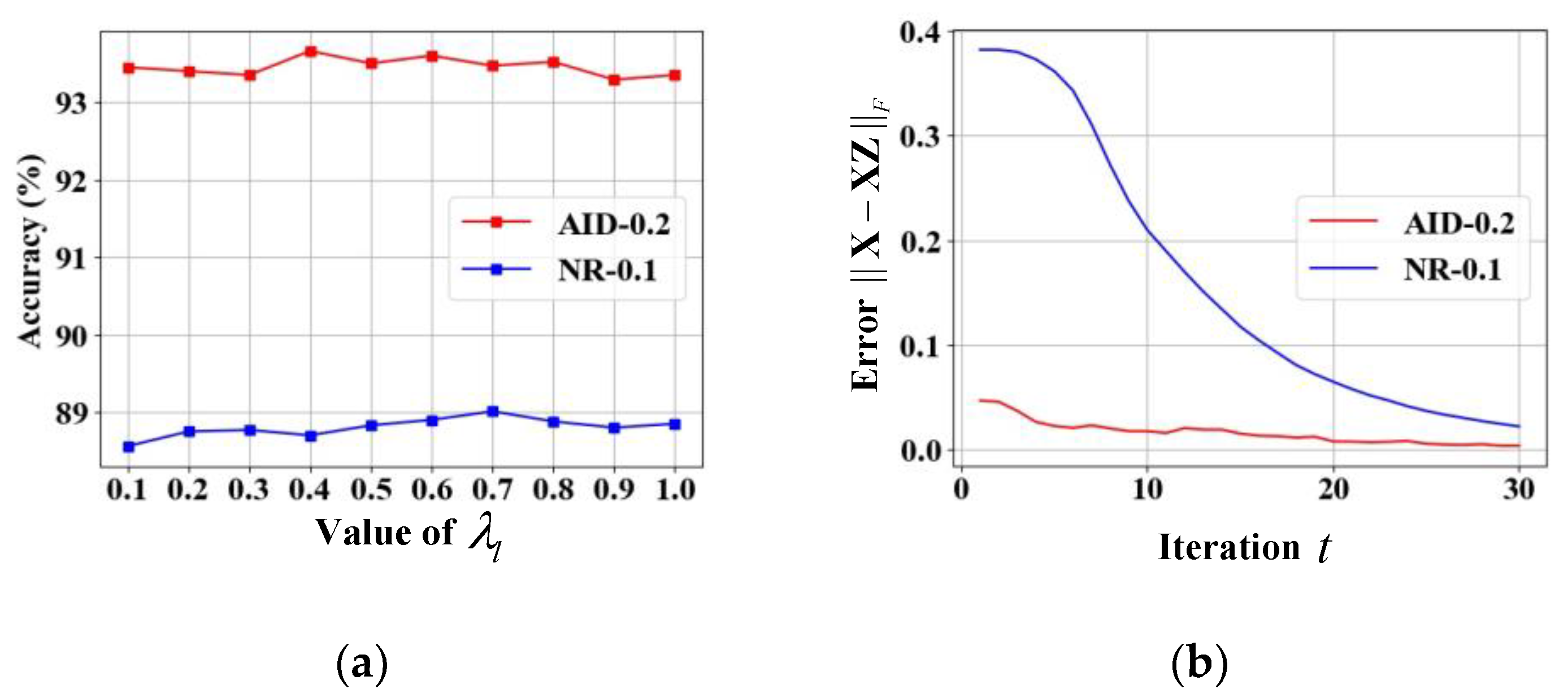
λ l controls the importance of the label distributions in the loss Function (14). For various values of λ l , the accuracies on testing sets are reported in Figure 16a. Our methods are insensitive to λ l within the interval [0.1, 1].

4.6.4. Time Efficiency

Table 5 summarizes the time consumptions of different steps for constructing our label distributions. Predefining label correlations consumes the most time because it includes the process of extracting sample features. It is fast to optimize the objective Function (3), and Figure 16b plots the convergence curves. The total time is relatively short and thus it is feasible to construct our label distributions for network training.

5. Discussion

5.1. Summary of the Experiment Results

According to the experiment results, the proposed N-LDL has the following advantages:
  • Our label distributions can robustly model label ambiguity for aerial images. Compared to D2LDL, our method substantially reduced label noise by incorporating label correlations, as shown in Figure 8.
  • Using our label distributions for network training yielded competitive classification performance. Compared to the label representations of LSR, CWL, or D2LDL, our label distributions led to higher accuracies, as presented in Table 3.
  • Our method can improve the generation ability of networks and is useful, especially for small datasets. Regularizing output distributions by our label distributions helps to mitigate over-fitting problems, as illustrated in Figure 13.
  • It is convenient and time-efficient to apply our method to common network structures. We only introduced label distributions to regularize network learning, and the time for constructing label distributions was short, as listed in Table 5.

5.2. Why Does N-LDL Work Well?

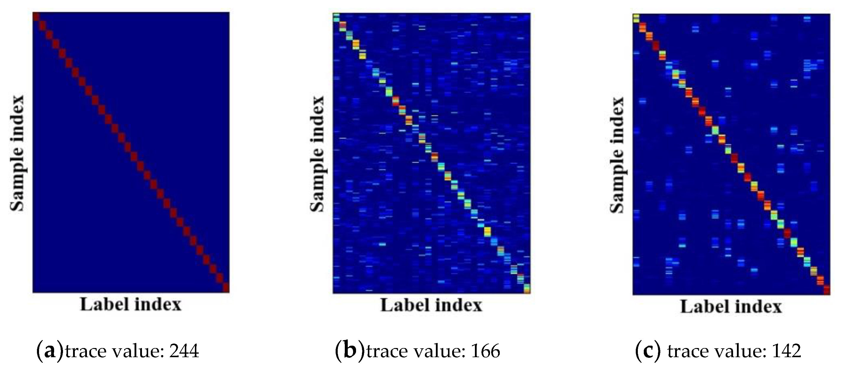
The label representations produced by N-LDL possess low trace values and can capture intrinsic label correlations. Literatures related to IncomLDL [32,33] and MLL [67,68] have proven that label representations considering label correlations contribute to improving classification performance. On the basis of low-rank assumption, a trace norm can be imposed on label representations to capture intrinsic label correlations [67]. Thus, the optimized label representations possess low trace values and can improve classification performance. Loosely speaking, label representations with low trace values enjoy strong ability to express label correlations. Figure 17 and Table 6 present the trace values of different label representations. From Table 5, the sample truth labels (i.e., Y) had the largest trace values due to the ignorance of label correlations. In contrast, N-LDL achieved the lowest trace values and thus can express label correlations sufficiently, which leads to the high OA, as listed in Table 3.

5.3. Are There Better Label Distributions?

The limitation of N-LDL is that the label distribution is fixed during network training, and we hope that the label distributions can be dynamically updated to further improve training processes. Equation (3) uses fixed global label correlations G to uncover sample neighbors and the constructed label distributions are fixed during CNN training. It is preferable to jointly learn label correlations, label distributions, and feature representations in a unified framework, which may be characterized by a trace norm and graph convolutional networks (GCNs) [69,70]:
  • As label distributions are expected to have low trace values, a trace norm can be imposed on network outputs (i.e., predicted label distributions) in loss functions, which enables the framework to be end-to-end trainable.
  • GCNs learned to map the initial label graph (such as the S or G in this paper) into inter-dependent label embeddings that can implicitly model label correlations. The label embeddings project sample features into network outputs, which enable the predicted label distributions to be consistent with label correlations.
In this paper, we fixed label distributions for network training, and it is convenient to apply N-LDL to various network structures. Experiment results demonstrated the effectiveness of the label distributions. In the future, we plan to build the unified framework that can alternatively update label distributions to further improve network training.

6. Conclusions

In this paper, we proposed neighbor-based label distribution learning (N-LDL) for aerial scene classification, in which subspace learning was adopted to uncover sample neighbors that cause label ambiguity. In subspace learning, the neighboring relations are regularized by a sparse constraint and the predefined label correlations, which jointly captures local similarity and label correlations. As a result, the uncovered neighbors shared correlated labels and the neighbor-based label distribution expressed the label ambiguity of samples. The experiment results demonstrated that using the label distributions for network training can mitigate over-fitting and assist feature learning, and our method yielded competitive classification performance. Additionally, the proposed method has the potential to model label ambiguity for generic single label learning (SLL) problems.

Author Contributions

Conceptualization, J.L.; Methodology, J.L. and Y.O.; Supervision, B.L.; Validation, B.H.; Writing—original draft, J.L.; Writing—review and editing, Y.W. All authors have read and agreed to the published version of the manuscript.

Funding

This research was funded by Major science and Technology Program of Sichuan Province, grant number 2018GZDZX0031.

Institutional Review Board Statement

Not applicable.

Informed Consent Statement

Not applicable.

Data Availability Statement

The aerial image dataset (AID) is downloadable at http://www.lmars.whu.edu.cn/xia/AID-project.html. The NWPU_RESISC45 (NR) is accessible at http://www.escience.cn/people/JunweiHan/NWPU-RESISC45.html.

Acknowledgments

The authors would like to express their gratitude to the editors and reviewers for their valuable comments and suggestions.

Conflicts of Interest

The authors declare no conflict of interest.

References

  1. Xia, G.S.; Hu, J.; Hu, F.; Shi, B.; Bai, X.; Zhong, Y.; Zhang, L.; Lu, X. AID: A benchmark data set for performance evaluation of aerial scene classification. IEEE Trans. Geosci. Remote Sens. 2017, 55, 3965–3981. [Google Scholar] [CrossRef] [Green Version]
  2. Cheng, G.; Han, J.; Lu, X. Remote Sensing Image Scene Classification: Benchmark and State of the Art. Proc. IEEE 2017, 105, 1865–1883. [Google Scholar] [CrossRef] [Green Version]
  3. Shao, Z.; Yang, K.; Zhou, W. A benchmark dataset for performance evaluation of multi-label remote sensing image retrieval. Remote Sens. 2018, 10, 964. [Google Scholar] [CrossRef] [Green Version]
  4. Ji, J.; Jing, W.; Chen, G.; Lin, J.; Song, H. Multi-label remote sensing image classification with latent semantic dependencies. Remote Sens. 2020, 12, 1110. [Google Scholar] [CrossRef] [Green Version]
  5. Shin, S.J.; Kim, S.; Kim, Y.; Kim, S. Hierarchical multi-label object detection framework for Remote Sensing Image. Remote Sens. 2020, 12, 2734. [Google Scholar] [CrossRef]
  6. Geng, X. Label Distribution Learning. IEEE Trans. Knowl. Data Eng. 2016, 28, 1734–1748. [Google Scholar] [CrossRef] [Green Version]
  7. Gao, B.B.; Xing, C.; Xie, C.W.; Wu, J.; Geng, X. Deep Label Distribution Learning with Label Ambiguity. IEEE Trans. Image Process. 2017, 26, 2825–2838. [Google Scholar] [CrossRef] [Green Version]
  8. Gao, B.B.; Zhou, H.Y.; Wu, J.; Geng, X. Age estimation using expectation of label distribution learning. In Proceedings of the International Joint Conference on Artificial Intelligence (IJCAI), Stockholm, Sweden, 13–19 July 2018; pp. 712–718. [Google Scholar]
  9. Yang, J.; Chen, L.; Zhang, L.; Sun, X.; She, D.; Lu, S.P.; Cheng, M.M. Historical context-based style classification of painting images via label distribution learning. In Proceedings of the 2018 ACM Multimedia Conference (MM 2018), Seoul, Korea, 22–26 October 2018; pp. 1154–1162. [Google Scholar]
  10. Xu, L.; Chen, J.; Gan, Y. Head pose estimation with soft labels using regularized convolutional neural network. Neurocomputing 2019, 337, 339–353. [Google Scholar] [CrossRef]
  11. Wu, X.; Wen, N.; Liang, J.; Lai, Y.K.; She, D.; Cheng, M.M.; Yang, J. Joint acne image grading and counting via label distribution learning. In Proceedings of the IEEE International Conference on Computer Vision, Seoul, Korea, 27 October–2 November 2019; pp. 10641–10650. [Google Scholar]
  12. Elhamifar, E.; Vidal, R. Sparse subspace clustering: Algorithm, theory, and applications. IEEE Trans. Pattern Anal. Mach. Intell. 2013, 35, 2765–2781. [Google Scholar] [CrossRef] [Green Version]
  13. Liu, G.; Lin, Z.; Yan, S.; Sun, J.; Yu, Y.; Ma, Y. Robust recovery of subspace structures by low-rank representation. IEEE Trans. Pattern Anal. Mach. Intell. 2013, 35, 171–184. [Google Scholar] [CrossRef] [PubMed] [Green Version]
  14. Adler, A.; Elad, M.; Hel-Or, Y. Linear-Time Subspace Clustering via Bipartite Graph Modeling. IEEE Trans. Neural Netw. Learn. Syst. 2015, 26, 2234–2246. [Google Scholar] [CrossRef]
  15. Von Luxburg, U. A tutorial on spectral clustering. Stat. Comput. 2007, 17, 395–416. [Google Scholar] [CrossRef]
  16. Wright, J.; Ma, Y.; Mairal, J.; Sapiro, G.; Huang, T.S.; Yan, S. Sparse representation for computer vision and pattern recognition. Proc. IEEE 2010, 98, 1031–1044. [Google Scholar] [CrossRef] [Green Version]
  17. Fang, X.; Han, N.; Wong, W.K.; Teng, S.; Wu, J.; Xie, S.; Li, X. Flexible Affinity Matrix Learning for Unsupervised and Semisupervised Classification. IEEE Trans. Neural Netw. Learn. Syst. 2019, 30, 1133–1149. [Google Scholar] [CrossRef]
  18. Li, C.G.; Vidal, R. Structured Sparse Subspace Clustering: A unified optimization framework. In Proceedings of the 2015 IEEE Computer Society Conference on Computer Vision and Pattern Recognition, Boston, MA, USA, 7–12 June 2015; pp. 277–286. [Google Scholar]
  19. Vidal, R.; Favaro, P. Low rank subspace clustering (LRSC). Pattern Recognit. Lett. 2014, 43, 47–61. [Google Scholar] [CrossRef] [Green Version]
  20. Fang, Y.; Wang, R.; Dai, B.; Wu, X. Graph-based learning via auto-grouped sparse regularization and kernelized extension. IEEE Trans. Knowl. Data Eng. 2015, 27, 142–154. [Google Scholar] [CrossRef]
  21. He, Z.; Li, X.; Zhang, Z.; Wu, F.; Geng, X.; Zhang, Y.; Yang, M.H.; Zhuang, Y. Data-Dependent Label Distribution Learning for Age Estimation. IEEE Trans. Image Process. 2017, 26, 3846–3858. [Google Scholar] [CrossRef]
  22. Yu, Y.; Li, X.; Liu, F. Attention GANs: Unsupervised Deep Feature Learning for Aerial Scene Classification. IEEE Trans. Geosci. Remote Sens. 2020, 58, 519–531. [Google Scholar] [CrossRef]
  23. Bi, Q.; Qin, K.; Li, Z.; Zhang, H.; Xu, K.; Xia, G.S. A Multiple-Instance Densely-Connected ConvNet for Aerial Scene Classification. IEEE Trans. Image Process. 2020, 29, 4911–4926. [Google Scholar] [CrossRef]
  24. Guo, Y.; Ji, J.; Lu, X.; Huo, H.; Fang, T.; Li, D. Global-Local Attention Network for Aerial Scene Classification. IEEE Access 2019, 7, 67200–67212. [Google Scholar] [CrossRef]
  25. Tong, W.; Chen, W.; Han, W.; Li, X.; Wang, L. Channel-Attention-Based DenseNet Network for Remote Sensing Image Scene Classification. IEEE J. Sel. Top. Appl. Earth Obs. Remote Sens. 2020, 13, 4121–4132. [Google Scholar] [CrossRef]
  26. Hashim, F.A.; Hussain, K.; Houssein, E.H.; Mabrouk, M.S.; Al-Atabany, W. Archimedes optimization algorithm: A new metaheuristic algorithm for solving optimization problems. Appl. Intell. 2020, 51, 1531–1551. [Google Scholar] [CrossRef]
  27. Pathak, Y.; Arya, K.V.; Tiwari, S. Feature selection for image steganalysis using levy flight-based grey wolf optimization. Multimed. Tools Appl. 2019, 78, 1473–1494. [Google Scholar] [CrossRef]
  28. Canayaz, M. MH-COVIDNet: Diagnosis of COVID-19 using deep neural networks and meta-heuristic-based feature selection on X-ray images. Biomed. Signal Process. Control 2021, 64, 102257. [Google Scholar] [CrossRef] [PubMed]
  29. Wang, J.; Geng, X. Classification with label distribution learning. In Proceedings of the IJCAI International Joint Conference on Artificial Intelligence, Honolulu, HI, USA, 27 January–1 February 2019; pp. 3712–3718. [Google Scholar]
  30. González, M.; González-Almagro, G.; Triguero, I.; Cano, J.R.; García, S. Decomposition-Fusion for Label Distribution Learning. Inf. Fusion 2021, 66, 64–75. [Google Scholar] [CrossRef]
  31. González, M.; Cano, J.R.; García, S. ProLSFEO-LDL: Prototype selection and label- specific feature evolutionary optimization for label distribution learning. Appl. Sci. 2020, 10, 3089. [Google Scholar]
  32. Xu, M.; Zhou, Z.H. Incomplete label distribution learning. In Proceedings of the International Joint Conference on Artificial Intelligence(IJCAI), Melboume, Australia, 19–25 August 2017; pp. 3175–3181. [Google Scholar]
  33. Jia, X.; Ren, T.; Chen, L.; Wang, J.; Zhu, J.; Long, X. Weakly supervised label distribution learning based on transductive matrix completion with sample correlations. Pattern Recognit. Lett. 2019, 125, 453–462. [Google Scholar] [CrossRef]
  34. Zeng, X.Q.; Chen, S.F.; Xiang, R.; Wu, S.X.; Wan, Z.Y. Filling missing values by local reconstruction for incomplete label distribution learning. Int. J. Wirel. Mob. Comput. 2019, 16, 314–321. [Google Scholar] [CrossRef]
  35. Zeng, X.Q.; Chen, S.F.; Xiang, R.; Li, G.Z.; Fu, X.F. Incomplete label distribution learning based on supervised neighborhood information. Int. J. Mach. Learn. Cybern. 2020, 11, 111–121. [Google Scholar] [CrossRef]
  36. Chen, K.; Kämäräinen, J.K.; Zhang, Z. Facial age estimation using robust label distribution. In Proceedings of the 2016 ACM Multimedia Conference (MM 2016), Amsterdam, The Netherlands, 15–19 October 2016; pp. 77–81. [Google Scholar]
  37. Ling, M.; Geng, X. Indoor Crowd Counting by Mixture of Gaussians Label Distribution Learning. IEEE Trans. Image Process. 2019, 28, 5691–5701. [Google Scholar] [CrossRef] [PubMed]
  38. Li, P.; Hu, Y.; Wu, X.; He, R.; Sun, Z. Deep label refinement for age estimation. Pattern Recognit. 2020, 100, 107178. [Google Scholar] [CrossRef]
  39. Ou, Y.; Luo, J.; Li, B.; Swamy, M.N.S. Gray-level image denoising with an improved weighted sparse coding. J. Vis. Commun. Image Represent. 2020, 72, 102895. [Google Scholar] [CrossRef]
  40. Zhuang, L.; Gao, S.; Tang, J.; Wang, J.; Lin, Z.; Ma, Y.; Yu, N. Constructing a Nonnegative Low-Rank and Sparse Graph With Data-Adaptive Features. IEEE Trans. Image Process. 2015, 24, 3717–3728. [Google Scholar] [CrossRef] [Green Version]
  41. Li, C.G.; You, C.; Vidal, R. Structured Sparse Subspace Clustering: A Joint Affinity Learning and Subspace Clustering Framework. IEEE Trans. Image Process. 2017, 26, 2988–3001. [Google Scholar] [CrossRef]
  42. Zhai, H.; Zhang, H.; Zhang, L.; Li, P.; Plaza, A. A new sparse subspace clustering algorithm for hyperspectral remote sensing imagery. IEEE Geosci. Remote Sens. Lett. 2017, 14, 43–47. [Google Scholar] [CrossRef]
  43. Chen, H.; Wang, W.; Feng, X. Structured Sparse Subspace Clustering with Within-Cluster Grouping. Pattern Recognit. 2018, 83, 107–118. [Google Scholar] [CrossRef]
  44. Wang, L.; Guo, S.; Huang, W.; Xiong, Y.; Qiao, Y. Knowledge Guided Disambiguation for Large-Scale Scene Classification With Multi-Resolution CNNs. IEEE Trans. Image Process. 2017, 26, 2055–2068. [Google Scholar] [CrossRef] [Green Version]
  45. Lei, Y.; Dong, Y.; Xiong, F.; Bai, H.; Yuan, H. Confusion Weighted Loss for Ambiguous Classification. In Proceedings of the 2018 IEEE International Conference on Visual Communications and Image Processing, Taichung, Taiwan, China, 9–12 December 2018. [Google Scholar]
  46. Chang, C.C.; Lin, C.J. LIBSVM: A Library for support vector machines. ACM Trans. Intell. Syst. Technol. 2011, 2, 27. [Google Scholar] [CrossRef]
  47. Boyd, S.; Parikh, N.; Chu, E.; Peleato, B.; Eckstein, J. Distributed optimization and statistical learning via the alternating direction method of multipliers. Found. Trends Mach. Learn. 2010, 3, 1–122. [Google Scholar] [CrossRef]
  48. Talukdar, P.P.; Crammer, K. New regularized algorithms for transductive learning. Lect. Notes Comput. Sci. 2009, 5782, 442–457. [Google Scholar]
  49. Müller, R.; Kornblith, S.; Hinton, G. When does label smoothing help? In Proceedings of the Advances in Neural Information Processing Systems, Vancouver, BC, Canada, 8–14 December 2019. [Google Scholar]
  50. Szegedy, C.; Vanhoucke, V.; Ioffe, S.; Shlens, J.; Wojna, Z. Rethinking the Inception Architecture for Computer Vision. In Proceedings of the 2016 IEEE Computer Society Conference on Computer Vision and Pattern Recognition, Las Vegas, NV, USA, 27–30 June 2016; pp. 2818–2826. [Google Scholar]
  51. Pereyra, G.; Tucker, G.; Chorowski, J.; Kaiser, Ł.; Hinton, G. Regularizing neural networks by penalizing confident output distributions. In Proceedings of the 5th International Conference on Learning Representations, Toulon, France, 24–26 April 2017. [Google Scholar]
  52. Hou, J.; Zeng, H.; Cai, L.; Zhu, J.; Chen, J.; Ma, K.K. Multi-label learning with multi-label smoothing regularization for vehicle re-identification. Neurocomputing 2019, 345, 15–22. [Google Scholar] [CrossRef]
  53. He, N.; Fang, L.; Li, S.; Plaza, A.; Plaza, J. Remote sensing scene classification using multilayer stacked covariance pooling. IEEE Trans. Geosci. Remote Sens. 2018, 56, 6899–6910. [Google Scholar] [CrossRef]
  54. Cheng, G.; Yang, C.; Yao, X.; Guo, L.; Han, J. When Deep Learning Meets Metric Learning: Remote Sensing Image Scene Classification via Learning Discriminative CNNs. IEEE Trans. Geosci. Remote Sens. 2018, 56, 2811–2821. [Google Scholar] [CrossRef]
  55. Yu, Y.; Liu, F. Dense connectivity based two-stream deep feature fusion framework for aerial scene classification. Remote Sens. 2018, 10, 1158. [Google Scholar] [CrossRef] [Green Version]
  56. Zhang, W.; Tang, P.; Zhao, L. Remote sensing image scene classification using CNN-CapsNet. Remote Sens. 2019, 11, 494. [Google Scholar] [CrossRef] [Green Version]
  57. Xie, J.; He, N.; Fang, L.; Plaza, A. Scale-free convolutional neural network for remote sensing scene classification. IEEE Trans. Geosci. Remote Sens. 2019, 57, 6916–6928. [Google Scholar] [CrossRef]
  58. He, N.; Fang, L.; Li, S.; Plaza, J.; Plaza, A. Skip-Connected Covariance Network for Remote Sensing Scene Classification. IEEE Trans. Neural Netw. Learn. Syst. 2020, 31, 1461–1474. [Google Scholar] [CrossRef] [Green Version]
  59. Xu, K.; Huang, H.; Deng, P.; Shi, G. Two-stream feature aggregation deep neural network for scene classification of remote sensing images. Inf. Sci. 2020, 539, 250–268. [Google Scholar] [CrossRef]
  60. Simonyan, K.; Zisserman, A. Very deep convolutional networks for large-scale image recognition. In Proceedings of the 3rd International Conference on Learning Representations, San Diego, CA, USA, 7–9 May 2015. [Google Scholar]
  61. He, K.; Zhang, X.; Ren, S.; Sun, J. Deep residual learning for image recognition. In Proceedings of the 2016 IEEE Computer Society Conference on Computer Vision and Pattern Recognition, Las Vegas, NV, USA, 27–30 June 2016; pp. 770–778. [Google Scholar]
  62. Bagherinezhad, H.; Horton, M.; Rastegari, M.; Farhadi, A. Label refinery: Improving ImageNet classification through label progression. arXiv 2018, arXiv:1805.06241. [Google Scholar]
  63. Liu, Z.; Chen, Z.; Bai, J.; Li, S.; Lian, S. Facial pose estimation by deep learning from label distributions. In Proceedings of the 2019 International Conference on Computer Vision Workshop, Seoul, Korea, 27 October 2 November 2019; pp. 1232–1240. [Google Scholar]
  64. Van Der Maaten, L.; Hinton, G. Visualizing data using t-SNE. J. Mach. Learn. Res. 2008, 9, 2579–2625. [Google Scholar]
  65. Xie, L.; Wang, J.; Wei, Z.; Wang, M.; Tian, Q. DisturbLabel: Regularizing CNN on the loss layer. In Proceedings of the 2016 IEEE Computer Society Conference on Computer Vision and Pattern Recognition, Las Vegas, NV, USA, 27–30 June 2016; pp. 4753–4762. [Google Scholar]
  66. Chen, B.; Deng, W.; Du, J. Noisy softmax: Improving the generalization ability of DCNN via postponing the early softmax saturation. In Proceedings of the 2017 IEEE Conference on Computer Vision and Pattern Recognition, Honolulu, HI, USA, 21–26 July 2017; pp. 4021–4030. [Google Scholar]
  67. Wu, B.; Jia, F.; Liu, W.; Ghanem, B.; Lyu, S. Multi-label Learning with Missing Labels Using Mixed Dependency Graphs. Int. J. Comput. Vis. 2018, 126, 875–896. [Google Scholar] [CrossRef] [Green Version]
  68. Zhu, C.; Miao, D.; Wang, Z.; Zhou, R.; Wei, L.; Zhang, X. Global and local multi-view multi-label learning. Neurocomputing 2020, 371, 67–77. [Google Scholar] [CrossRef]
  69. Chen, Z.M.; Wei, X.S.; Wang, P.; Guo, Y. Multi-label image recognition with graph convolutional networks. In Proceedings of the IEEE Computer Society Conference on Computer Vision and Pattern Recognition, San Diego, CA, USA, 16–20 June 2019; pp. 5172–5181. [Google Scholar]
  70. Liu, Y.; Chen, W.; Qu, H.; Mahmud, S.M.H.; Miao, K. Weakly supervised image classification and pointwise localization with graph convolutional networks. Pattern Recognit. 2021, 109, 107596. [Google Scholar] [CrossRef]
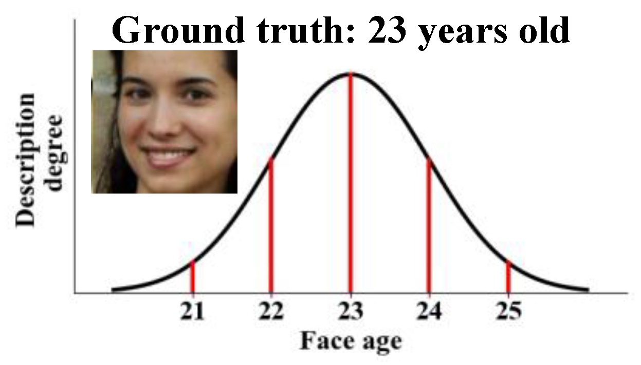
Figure 1. Gaussian-based label distribution of an age image. The face image comes from the dataset of Chalearn 2015 [7].
Remotesensing 13 00755 g001
Figure 2. Fundamental idea of this paper.
Remotesensing 13 00755 g002
Figure 3. Flowchart of our method.
Remotesensing 13 00755 g003
Figure 4. Soft mappings from label similarities S to label differences G.
Remotesensing 13 00755 g004
Figure 5. Example images of the datasets: (a) AID and (b) NR.
Remotesensing 13 00755 g005
Figure 6. Grouped label distributions of Rail S samples. At the left, each row represents the label distribution of a sample. At the right, we present the images of which the label distributions near the corresponding cluster centers.
Remotesensing 13 00755 g006
Figure 7. Visualizations of (a) the global label correlations G and (b) the affinity graph A. Because the AID-0.2 dataset is comprised of 2000 training samples that cover 30 scene classes, A is a 2000 × 2000 matrix and G is a 30 × 30 matrix. The dark and light colors stand for low and high values, respectively. The dark elements in G indicate low label differences, and the light elements in A represents strong neighboring relations.
Remotesensing 13 00755 g007
Figure 8. Label distributions produced by (a) D2LDL that leads to N d = 411 and (b) our method that leads to N d = 138 . Since the training sample of AID-0.2 is too numerous (2000), we display only 10 samples per scene, and each row in the figure represents the label distribution of a sample. N d is the number of distorted distributions in all 2000 samples.
Remotesensing 13 00755 g008
Figure 9. Distorted distributions produced by our method.
Remotesensing 13 00755 g009
Figure 10. Confusion matrices on AID-0.1 that are obtained using (a) D2LDL-v and (b) N-LDL-v. Elements smaller than 0.01 are omitted.
Remotesensing 13 00755 g010
Figure 11. Two-dimensional representations of image features. The images come from the testing set of AID-0.2.
Remotesensing 13 00755 g011
Figure 12. Learning curves of original VGG and N-LDL-v on (a) AID-0.2, (b) Aug AID-0.2, and (c) AID-0.5.
Remotesensing 13 00755 g012
Figure 13. Classification results using different sizes of training sets on datasets of (a) AID and (b) NR.
Remotesensing 13 00755 g013
Figure 14. Label distributions that are produced by our method using different α z . (a) when α z = 0.1 , N d = 318 ; (b) when α z = 0.5 , N d = 162 ; (c) when α z = 2 , N d = 76 ; (d) when α z = 10 , N d = 5 . N d denotes the number of distorted distributions in all training samples.
Remotesensing 13 00755 g014
Figure 15. Influence of different feature dimensions, D. The left and right vertical coordinates represent the time consumption for solving Equation (3) and the classification accuracy, respectively. The experiments are conducted on AID-0.2 using 4096-dimensional VGG features.
Remotesensing 13 00755 g015
Figure 16. Analysis of (a) the trade-off parameter λ l and (b) the convergence of the subspace learning.
Remotesensing 13 00755 g016
Figure 17. Different label representations and their individual trace values on AID-0.2: (a) Sample truth labels, (b) D2LDL-v, and (c) N-LDL-v.
Remotesensing 13 00755 g017
Table 1. Symbol descriptions.
SymbolDescription
NThe number of training samples
CThe number of labels
DThe dimension of the sample features
y n The ground truth of the nth sample
Y R C × N The binary matrix of sample truth labels
X R D × N The set of sample features
G R C × C The matrix of global label correlations
Z R N × N The matrix of representation coefficients
A R N × N The sample affinity graph
P R C × N The set of label distributions
P r R C × N The set of rectified label distributions
Table 2. Methods for constructing label representations of training samples.
MethodDescription
Original CNNsSample ground truth is used to train original VGG and ResNet.
Label smoothing regularization (LSR) [50,52]LSR is the standard label smoothing method, which handles label ambiguity by uniform label smoothing. The smoothing parameter to 0.1.
Confusion weighted loss (CWL) [44,45] CWL [44,45] encodes label ambiguity on the basis of the confusion matrices on validation sets. Label pairs with high confusion proportions are posited to be correlated, and the label intensity is smoothed from sample ground truth to the correlated labels. The label representations are class-specific. We set the confusion thresholds [45] for AID and NR as 0.02 and 0.03 respectively, due to the lower accuracy achieved on NR.
D2LDLD2LDL constructs neighbor-based label distributions but overlooks label correlations. The label distributions are rectified by Equation (13).
N-LDLN-LDL jointly captures local similarity and label correlations. The label distributions are rectified by Equation (13).
Table 3. OA (%) comparisons using various label representations.
MethodAID-0.2NR-0.1
VGG91.21 ± 0.2885.90 ± 0.22
LSR-v91.93 ± 0.2186.66 ± 0.16
CWL-v92.79 ± 0.3587.32 ± 0.28
D2LDL-v92.61 ± 0.2687.29 ± 0.17
N-LDL-v (ours)93.66 ± 0.2388.58 ± 0.20
ResNet92.61 ± 0.2688.09 ± 0.23
LSR-r93.10 ± 0.2288.41 ± 0.17
CWL-r93.68 ± 0.3188.95 ± 0.27
D2LDL-r93.51 ± 0.2589.01 ± 0.18
N-LDL-r (ours)94.11 ± 0.2289.80 ± 0.19
‘-v’ and ‘-r’ indicate backbones of VGG and ResNet, respectively. The bold font denotes the best performance conditioned on the same backbones.
Table 4. OA (%) comparisons with state-of-the-art methods.
MethodsYearAID-0.2NR-0.1
MSCP [53]201891.52 ± 0.2185.33 ± 0.17
D-CNN [54]201890.82 ± 0.1689.22 ± 0.50
TEX-TS-Net [55]201893.31 ± 0.1184.77 ± 0.24
CapsNet [56]201993.79 ± 0.1389.03 ± 0.21
SF-CNN [57]201993.60 ± 0.1289.89 ± 0.16
SCCov [58]202093.12 ± 0.2589.30 ± 0.35
Attention-GAN [22]202093.97 ± 0.2388.06 ± 0.19
MIDC-Net [23]202088.51 ± 0.4186.12 ± 0.29
TFADNN [59]202093.21 ± 0.3287.78 ± 0.11
N-LDL-r (ours) 94.11 ± 0.2289.80 ± 0.19
The bold font denotes the method achieving the best performance. Explanations of Acronyms: multilayer stacked covariance pooling (MSCP) [53], discriminative CNN (D-CNN) [54], texture coded two-stream network (TEX-TS-Net) [55], capsule network (CapsNet) [56], scale-free (SF-CNN) [57], skip-connected covariance network (SCCOV) [58], attention generative adversarial network (Attention-GAN) [22], multiple-instance densely-connected network (MIDC-Net) [23], Two-stream feature aggregation deep neural network (TFADNN) [59].
Table 5. Time consumption (s) for constructing the label distributions of all the training samples.
DatasetStep 1Step 2Step 3Total Time
AID-0.255.26.50.662.3
NR-0.149.622.00.872.4
Step 1: predefining label correlations, Step 2: optimizing the objective Function (3), Step 3: label propagation and rectification.
Table 6. Trace values of different label representations.
Sample Truth LabelsD2LDL-vN-LDL-vD2LDL-rN-LDL-r
AID-0.2244.03166.74142.27162.30110.54
NR-0.1376.12183.51155.15179.28124.67
Publisher’s Note: MDPI stays neutral with regard to jurisdictional claims in published maps and institutional affiliations.