Article

Cloud and Cloud-Shadow Detection for Applications in Mapping Small-Scale Mining in Colombia Using Sentinel-2 Imagery

1
Minerals Engineering, Materials & Environment (GeMMe), University of Liège, 4000 Liège, Belgium
2
The College of Forestry, Beijing Forestry University, Beijing 100083, China
3
United Nations Environment Programme, Bogota Cl. 82 #10-62, Colombia
4
Institute for Environmental Sciences, University of Geneva, GRID-Geneva, Bd Carl-Vogt 66, CH-1211 Geneva, Switzerland
5
Institute for Environmental Sciences, University of Geneva, EnviroSPACE Lab., Bd Carl-Vogt 66, CH-1211 Geneva, Switzerland
*
Author to whom correspondence should be addressed.
Remote Sens. 2021, 13(4), 736; https://doi.org/10.3390/rs13040736
Submission received: 8 January 2021 / Revised: 10 February 2021 / Accepted: 13 February 2021 / Published: 17 February 2021

Abstract

:
Small-scale placer mining in Colombia takes place in rural areas and involves excavations resulting in large footprints of bare soil and water ponds. Such excavated areas comprise a mosaic of challenging terrains for cloud and cloud-shadow detection of Sentinel-2 (S2A and S2B) data used to identify, map, and monitor these highly dynamic activities. This paper uses an efficient two-step machine-learning approach using freely available tools to detect clouds and shadows in the context of mapping small-scale mining areas, one which places an emphasis on the reduction of misclassification of mining sites as clouds or shadows. The first step is comprised of a supervised support-vector-machine classification identifying clouds, cloud shadows, and clear pixels. The second step is a geometry-based improvement of cloud-shadow detection where solar-cloud-shadow-sensor geometry is used to exclude commission errors in cloud shadows. The geometry-based approach makes use of sun angles and sensor view angles available in Sentinel-2 metadata to identify potential directions of cloud shadow for each cloud projection. The approach does not require supplementary data on cloud-top or bottom heights nor cloud-top ruggedness. It assumes that the location of dense clouds is mainly impacted by meteorological conditions and that cloud-top and cloud-base heights vary in a predefined manner. The methodology has been tested over an intensively excavated and well-studied pilot site and shows 50% more detection of clouds and shadows than Sen2Cor. Furthermore, it has reached a Specificity of 1 in the correct detection of mining sites and water ponds, proving itself to be a reliable approach for further related studies on the mapping of small-scale mining in the area. Although the methodology was tailored to the context of small-scale mining in the region of Antioquia, it is a scalable approach and can be adapted to other areas and conditions.

Graphical Abstract

1. Introduction

Informal small-scale alluvial gold mining, also known as placer mining, has major social and environmental impacts and has been at the heart of complicated armed conflicts in various parts of the world. It is distinct from subsistence mining as it utilizes large machinery to excavate soil and river sediment [
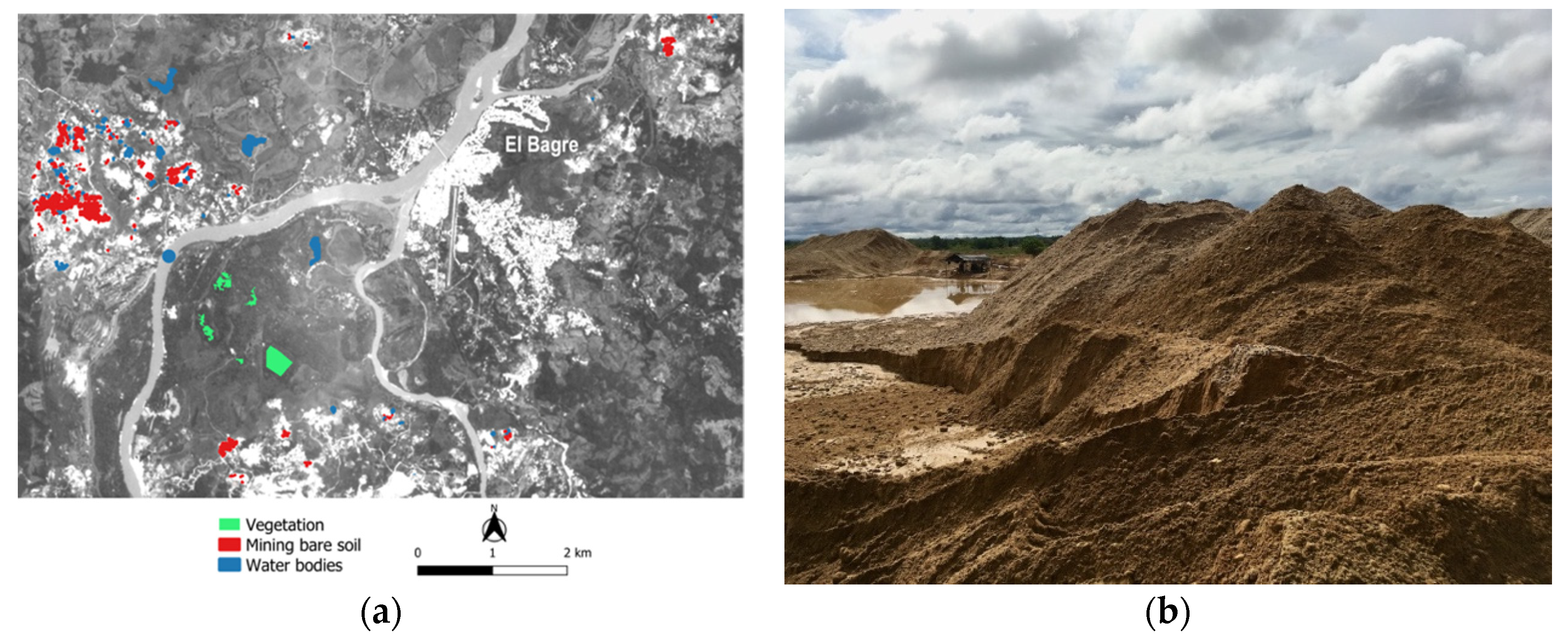
1]. When carried out on the riverbanks, it leaves large footprints of bare soil along with ponds of water that are utilized for on-site processing [2,3]. Such ponds are required to pump ore slurry and wash it through sluice boxes under pressure where the gold particles are collected. Prior to the 2018 mercury ban [4], amalgamation was intensively used to improve the capture of the finest gold particles leading to major health hazards [5]. This law was implemented for the mining sector, but it has not been well enforced, resulting in illegal mercury markets that supply illegal/informal mining [6].
A small-scale placer mining activity is considered formal/legal when the operator obtains a mining title and a program of works (Programa de Trabajos y Obras—PTO). Accordingly, the small-scale mining activities are required to be less than 150 hectares and need strict measures of land recovery [1]. Unfortunately, it is estimated that more than 70% of the gold production in Colombia is extracted from informal small- and medium-scale activities where the operators have not obtained legal permissions to do so [7,8,9]. This situation has worsened with the increase in gold prices since the year 2000. Despite the major environmental and social impacts of these activities, the fact remains that traditional land surveys are very challenging for such remote and harsh areas as they lack suitable spatial or temporal coverage. Earth observation techniques can be an improved method to detect, map, and monitor these extractive activities and assess their impacts [5,10,11,12].
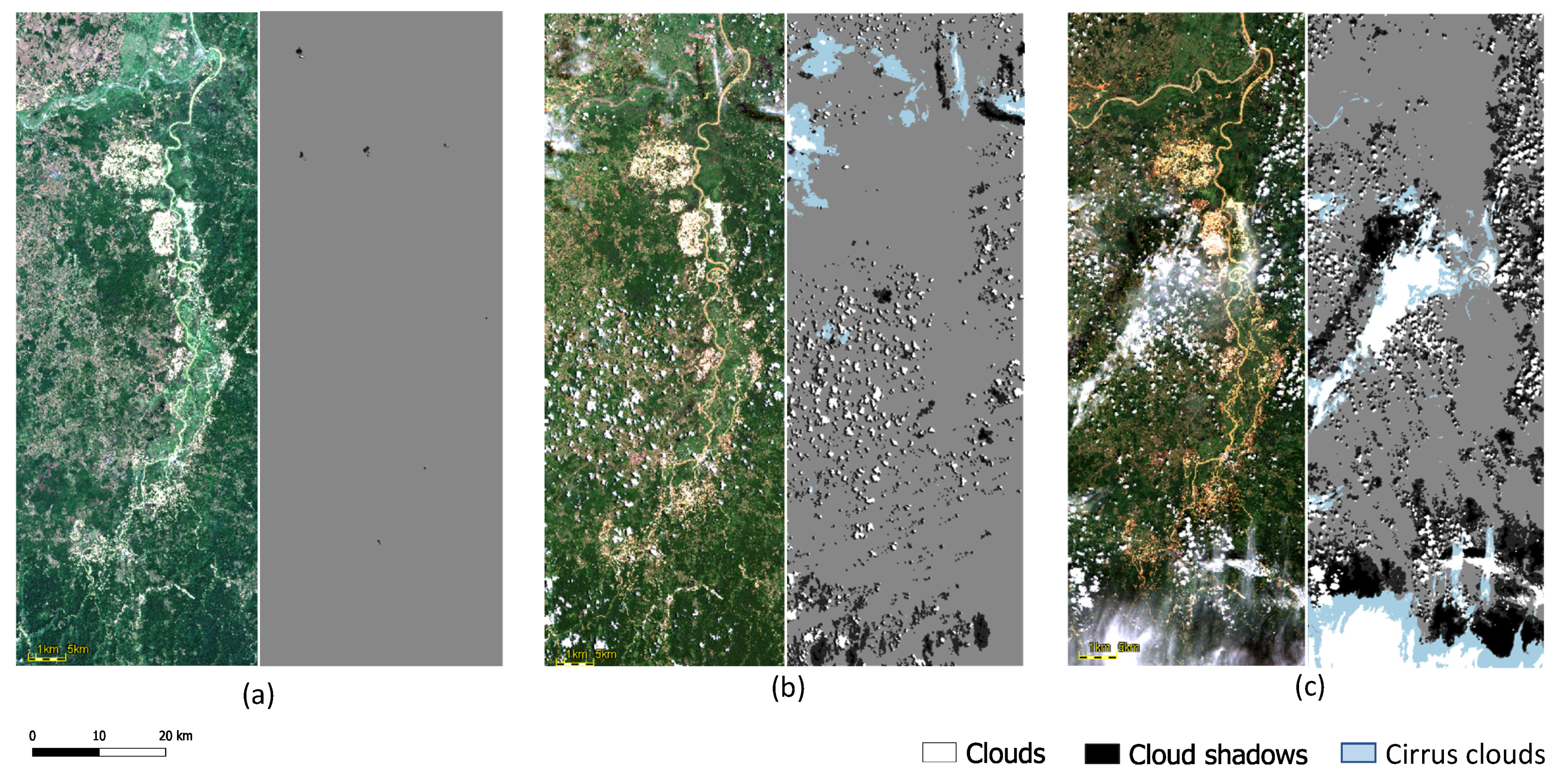
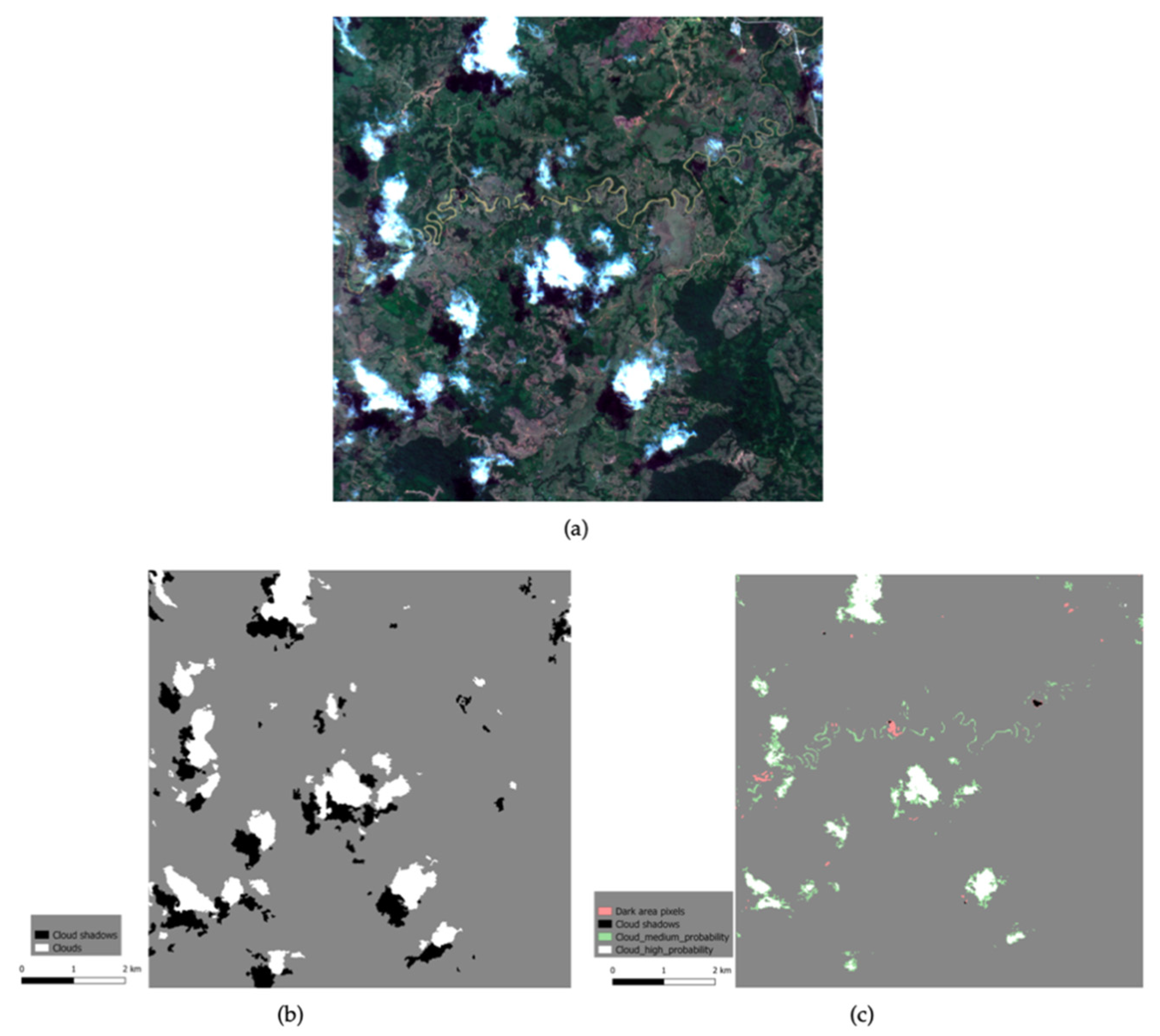
When utilizing optical spaceborne data, cloud coverage can be a hindering factor for analysis methods where cloud and cloud-shadow detection is essential prior to using the imagery. Unfortunately, the footprints of bare excavated areas are of relatively high reflectance; and along with water ponds, they comprise a mosaic of challenging terrains for cloud and cloud-shadow detection [13,14]. There are three major categories of clouds that affect imagery in different manners, namely cumulus, stratus, and cirrus clouds. Cumulus and stratus clouds, often referred to as dense clouds, are the lowest clouds. They have relatively high reflectance and can be easier to detect in satellite imagery than higher cirrus clouds that appear as detached filaments [15]. Approaches to detect these dense clouds and their shadows can vary. For example, each satellite scene can be studied separately, i.e., a mono-temporal approach [16,17,18,19,20,21,22,23,24,25], or a time series of images is used to identify clouded pixels of relatively higher reflectance, i.e., a multi-temporal methodology [26,27]. On the other hand, any cloud shadows depicted in an image are projections of corresponding clouds, and thus, the direction of observations plays a large role in the location and geometry of the shadows [28]. This cause-and-effect relationship between a cloud and its shadow is to be considered essential in their detection [22]. Various cases have been reported regarding the challenges of relying only on spectral information in detecting cloud shadows where false positive detection can easily occur due to topographical features or water bodies [13]. Accordingly, thermal data, textural characteristics, or geometric characteristics of cloud shadows have been utilized for improved detection [23,28,29,30]. Other approaches to monitor clouded areas involve the use of synthetic aperture radar (SAR) data, i.e., not affected by clouds, such as the data acquired by Sentinel-1 of the Copernicus program [31,32].
The advantage of using the Copernicus Sentinel-2 constellation of two satellites (S2A and S2B) is that its data are freely available and have a 10m resolution for various bands. The Multispectral Instruments (MSIs) are the sensors on-board of the satellites, with the first data acquisitions dating to 2016. The combined use of the two platforms allows a high revisit time, with an image over Colombia obtained every 5 days. MSIs provide images with thirteen bands. The central wavelength (λ) and bandwidth of each band per sensor are detailed in Table 1. Depending on the band (B), Sentinel-2 data can have a spatial resolution of 10m, 20m, or 60m [33].
A popular source of atmospherically corrected Sentinel-2 (S2) data for Colombia is the Copernicus hub (https://scihub.copernicus.eu/) that utilizes Sen2Cor, a semi-empirical mono-temporal model for radiometric and atmospheric correction. Using Sen2Cor, the L1C level of the data, i.e., the top of the atmosphere radiance, is transformed into Level L2A, which corresponds to surface reflectance. Cloud (dense and cirrus clouds) and shadow detection are available for L1C and L2A products [19,34,35]. For L1C data, dense cloud detection utilizes B2 (490nm) and with the help of shortwave infra-red (SWIR) B10 (1375 nm), B11 (1610 nm), and B12 (2190 nm), the false inclusion of snow is avoided. B10 is also used for the detection of cirrus clouds as their high altitude can be detected using a band with high atmospheric absorption. Finally, filters applied on detected clouds are used to remove isolated pixels and to fill gaps within clouds [35]. On the other hand, cloud detection for L2A products utilizes several steps of threshold filtering using indices that involve land cover to avoid detecting false cloud pixels in regions of possible false detection, such as areas of bare soil [36]. Unfortunately, the cloud detection approach of Sen2Cor has been reported to result in the unsatisfactory detection of dense clouds and their shadows [14,24,37], and has been shown to result in false positives in small-scale mining areas [12].
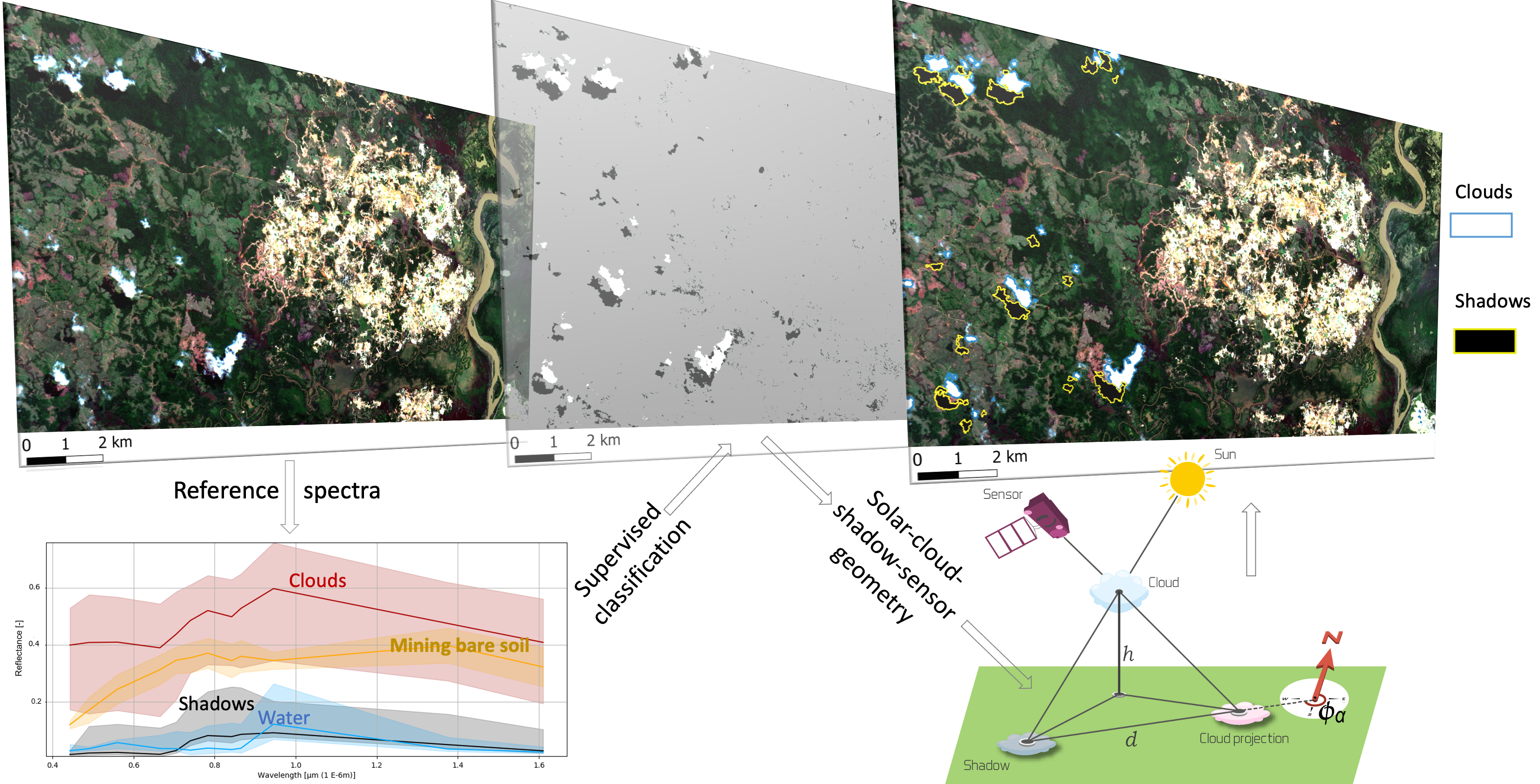
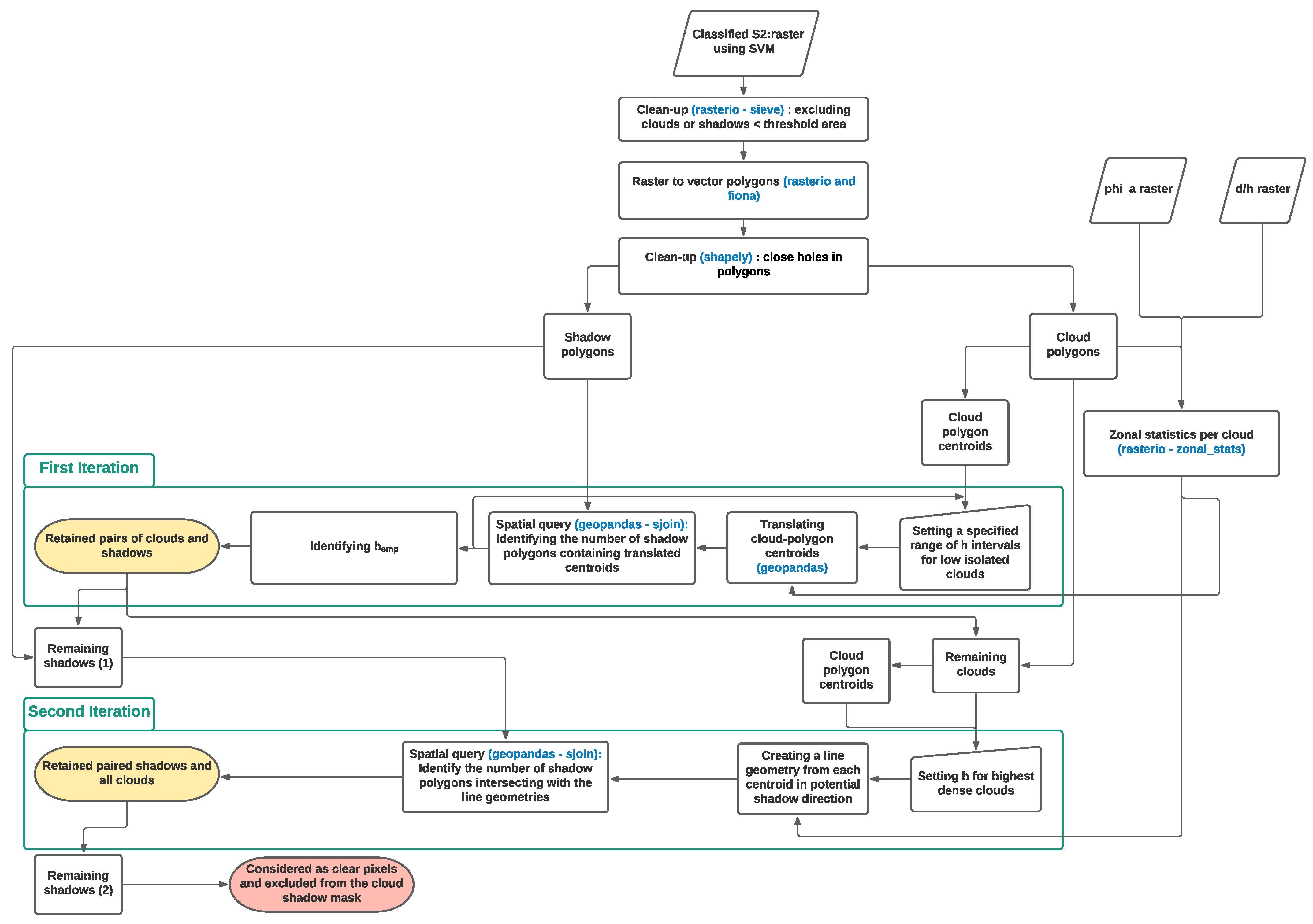
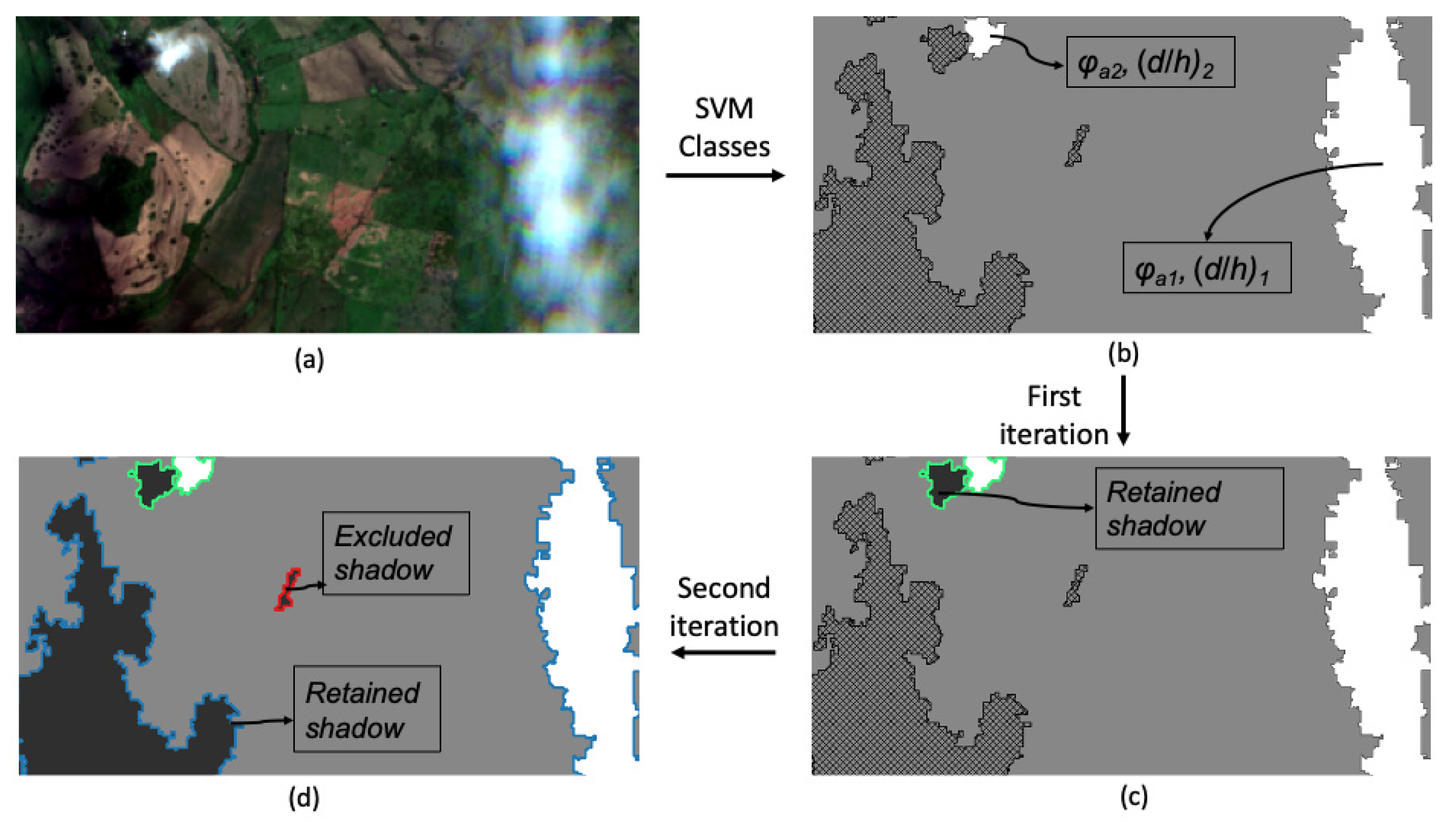
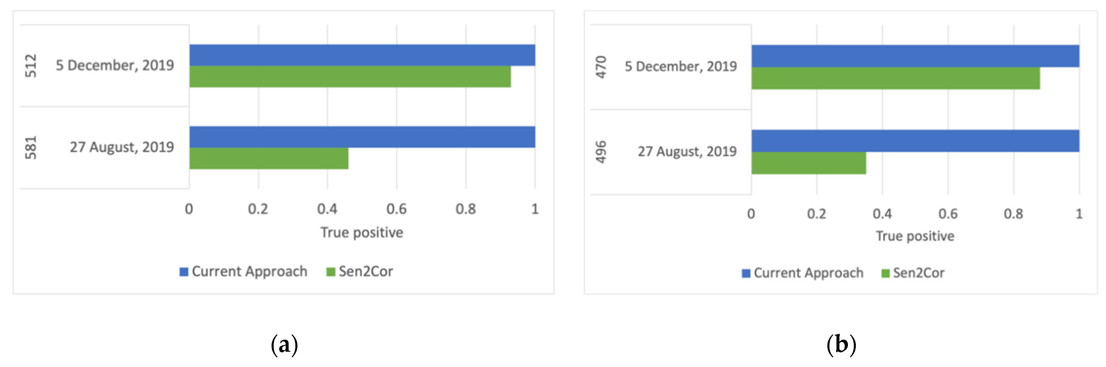
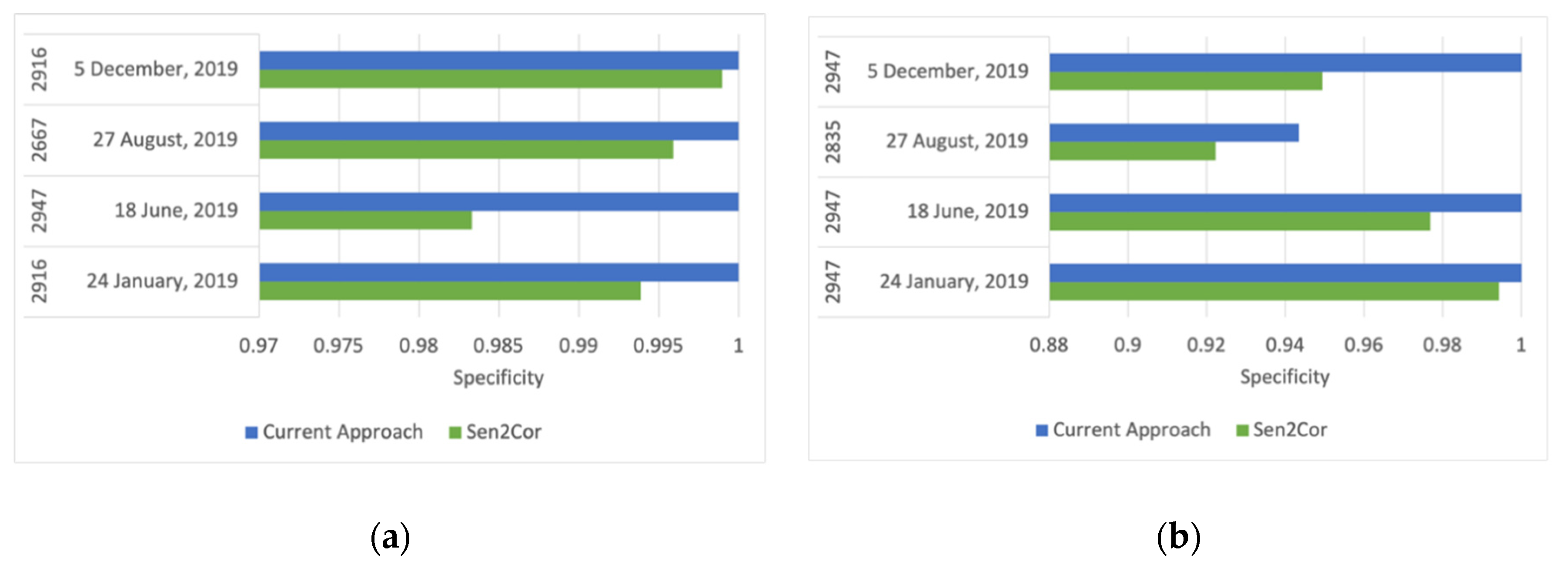
This paper aims to provide improved cloud and shadow detection in an approach that is simple, efficient, and based on freely available tools. It aims at improving cloud and cloud shadow detection in the context of mapping small-scale mining where the areas of interest are bare soil and water ponds. This procedure consists of two consecutive machine-learning steps. First, a supervised classification detects candidate clouds and shadows; second, the solar-cloud-shadow-sensor geometry and a causality effect between cloud shadows and clouds are considered to reduce shadow commission error. There have been already various methods developed that include the reduction of cloud-shadow false positives. One “universal” method that can be used for Sentinel-2 data considers an object-based image analysis approach for shape spatial-matching of cloud and cloud–shadows [22]. Another approach developed for MODIS data considers a geometry-based tool to detect potential shadows followed by classification to match the two outputs [13]. Other geometry-based approaches have been tailored for specific sensors that include thermal bands [28,38].
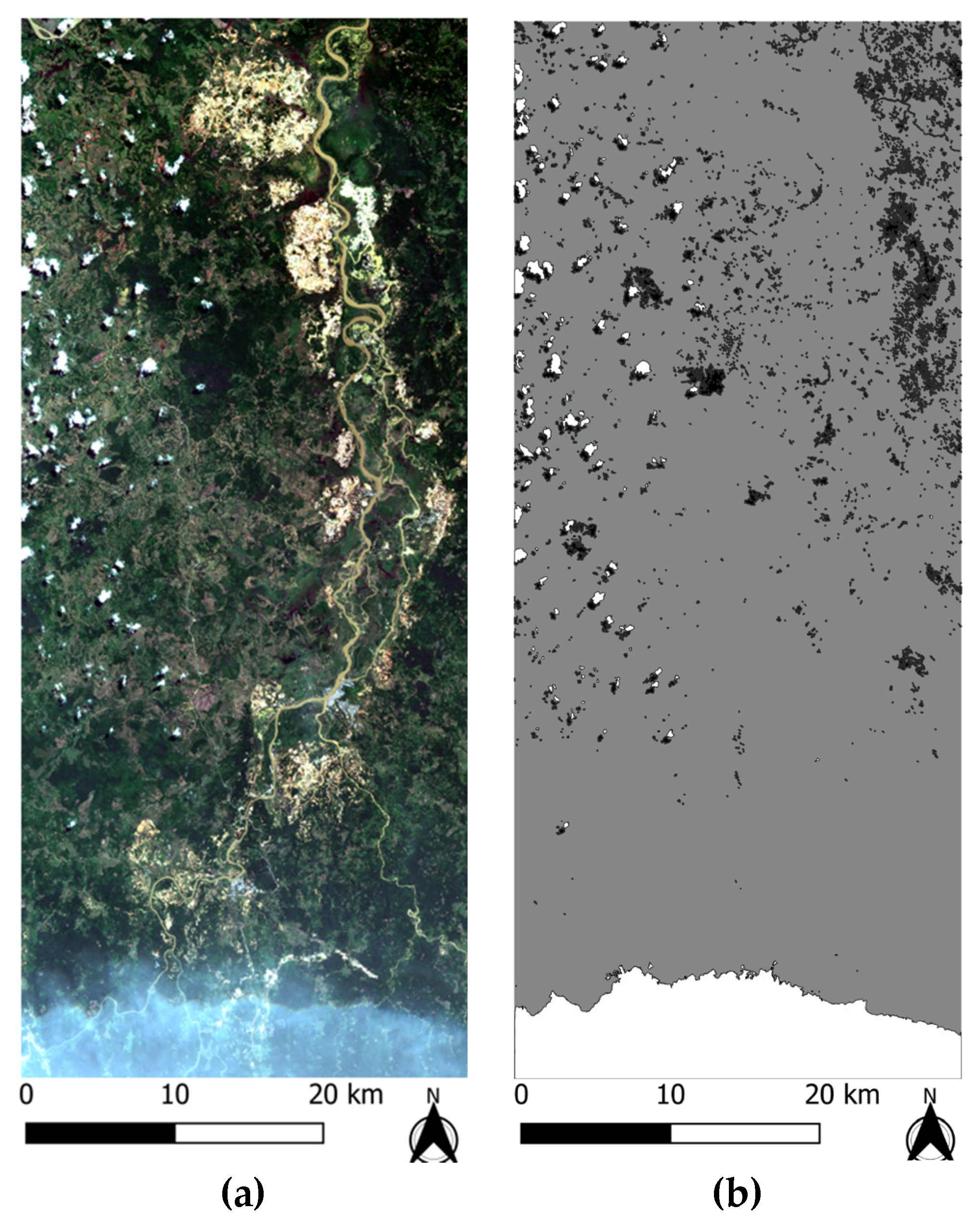
This paper proposes a simple pixel-based approach that provides a high-quality identification of clouds and their shadows for Sentinel-2 in the context of small-scale mining in Colombia. This work aims to efficiently provide a suitable tradeoff between omission errors leading to failure in excluding contaminated pixels and commission errors that result in masking out clear pixels. Although the methodology was tailored for the setting of the study area in the context of small-scale mining, it is scalable and can be a solid basis to develop a more generalized approach. The methodology is tested over an intensively excavated region through a mono-temporal approach due to the highly dynamic characteristics of the excavated areas and the rapid landcover change that needs to be depicted. A validation of the results using images acquired in different seasons was carried out on a well-studied pilot site in the vicinity of the town of El Bagre [5]. The success of this approach is a milestone for time series analysis of land cover around mining sites that will lead to an early warning system about the sprawl of excavations, especially in the vicinity of protected or sensitive areas. Such important output is to be shared with stakeholders through MapX (https://mapx.org), an online information and engagement platform that would allow the consolidation of data, analysis, and spatial visualization [39]. MapX was developed by the United Nations Environment Program (UNEP) and UNEP/ GRID-Geneva (https://unepgrid.ch).

2. Study Area

The study area is in the department of Antioquia along the path of the Nechí river. This department is the main producer of gold in Colombia, and the abundance of placer mining in the area makes it an optimal site to test remote sensing applications. Figure 1a shows the location of the study area with respect to Antioquia and Colombia and (b) a Red-Green-Blue (RGB) view of the area using a Sentinel-2 (S2B) image acquired on 18 June 2019, with an indication of the pilot-site location around the town of El Bagre at latitude 7°36’17.88’’N and longitude 74°48’32.32’’W. The area includes water bodies (rivers, isolated bodies, etc.), non-vegetated regions (built-up areas, mining areas, bare soil, etc.), and vegetated regions (forests, shrubs, agriculture, etc.). Figure 1c shows the topography of the area using a Digital Elevation Model (DEM) from the Shuttle Radar Topography Mission (SRTM) (1 arc-second resolution), freely available through the United States Geological Survey (http://earthexplorer.usgs.gov/). The elevation ranges from 30 m to 500 m and is relatively smooth along the river with slightly rugged areas limited to the southern part. The average elevation along the riverbanks where the land excavations take place does not exceed 60 m. The study area has a tropical warm-humid climate with frequent cloud coverage. The region experiences a dry season from December to March and a rainy season the rest of the year. It has a relatively spatially homogeneous climate with an average annual temperature around 28 °C and seasonal temperature variability of approximately 5 °C (Figure 2). The closest weather station within consistent topography and providing data through WeatherUnderground.com is at Los Garzones International Airport Station, about 175 km from the town of El Bagre and at 15 m of elevation (Figure 2).

3. Methodology

3.1. Classification for Dense Cloud and Shadow Detection

Dense clouds have high reflectance in the visible part of the spectrum. This can cause misclassification of land-cover of high brightness as clouds [14,40]. In fact, this has been observed in the study area where bare soil and highly turbid shallow ponds of small-scale mining have been misidentified. On the other hand, areas shadowed by clouds are relatively dark due to lower irradiance, and thus can be misclassified as water bodies and areas shaded by topographical features and vice versa [30,40]. Since the topography of the study area is generally smooth, such topographical impacts on alluvial mining sites can be considered minimal. Figure 3 shows examples of reflectance spectra, whereby it shows the mean spectrum (± standard deviation) of a selected cloud and its shadow along with a nearby mining site and water body. These spectra were extracted from the Sentinel-2 (S2B) image of the study area acquired on 18 June 2019. The reflectance of cloud and mine bare-soil pixels is relatively high with distinction depicted at band 1 and band 9 located in the water vapor absorption regions [19]. On the other hand, water and shadow pixels show low reflectance throughout the spectrum.
A supervised classification approach is used to identify three classes: clouds, cloud shadows, and clear pixels. The Sentinel-2 image acquired on 18 June 2019 (Figure 1) is used to extract reference spectra because it includes clouds and shadows over various landcovers along the western and southern regions (Table 2). These reference spectra are available as Supplementary Materials data with this manuscript. A Support-Vector-Machine (SVM) classifier is used as it has proven its suitability for landcover classification in diverse areas [41,42,43], for small-scale mining detection at the pilot site [5], and for cloud-shadow detection [13]. SVM is implemented using “Scikit-learn: Machine Learning in Python” [44] where it aims to find an optimal hyperplane separating the data into the pre-specified classes, and “kernels” can be used to introduce new variables that improve class separability [45]. The commonly used kernel functions include Linear and Radial Basis Function (RBF-Gaussian) kernels, and they require optimization parameters. Both types of kernels use “C” (penalty for misclassification) that allows for modification in the rigidity of training data. The RBF kernel also requires “gamma” (reflecting the spread of the kernel) that impacts the smoothing of the hyperplane shape [42]. Larger values of “C” may lead to an over-fitting model, whereas increasing “gamma” will affect the shape of the class-dividing hyperplane, which may affect the classification accuracy. To identify the most suitable parameters, the grid-search method is used, where “gamma” [1, 0.1, 0.01] and “C” [1, 50, 100, 200]. The parameter values are tested using a three-fold cross-validation approach, and those resulting in the highest classification accuracy are selected. Classification accuracy is reported as precision value Pr = T/(T + F), where T is the number of true positives and F the number of false positives.
As SVM can handle the dimensionality of the Sentinel-2 data, the use of all 12 bands is possible. Furthermore, as water bodies are of concern in the analysis, the indices that have been proven to be powerful in the detection of water and distinguishing it from other landcovers are tested. The features include the Normalized Difference Vegetation Index (NDVI) (B8-B4)/(B8+B4) and Modified Normalized Difference Water Index (MNDWI) (B3-B11)/(B3+B11) [46,47,48]. As B1 and B9 reflectance is relatively higher for clouds than for mining areas, one more test is considered where features are reduced to only bands 1 and 9 along with NDVI and MNDWI,

3.2. Geometry-Based Improvement of Cloud Shadow Detection

3.2.1. Direction of Cloud Shadow with Respect to Cloud Projection

Sentinel-2’s orbit is sun-synchronous where the twin satellites follow the same orbit at a mean altitude of 786 km but 180 degrees apart. They acquire the data at Mean Local Solar Time of 10:30 a.m. at the descending mode [50]. Cloud shadow locations with respect to cloud projection in imagery are dependent on the direction of solar radiation represented by solar zenith and azimuth angles, and by the sensor viewing geometry along with cloud top and bottom height [28,29,40,46,51]. Except for cloud height, all parameters are available in the Sentinel-2 image metadata. Accordingly, the direction of cloud shadow (Figure 4), referred to as Apparent Solar Azimuth (φa) can be estimated [40,51]:
tan(φa) = (sinφstanθssinφvtanθv) / (cosφstanθscosφvtanθv)
where φs and θs are the solar azimuth and zenith angles, respectively; φv and θv are the sensor’s view azimuth and zenith angles, respectively. As φa can have two possible angles with a difference of π radians, the angle is selected to be the one opposite to the sun’s mean azimuth location on the image. As the images are acquired before noon, it is expected that φa [180, 360]. Sentinel-2 metadata provide mean φs and mean θs. Yet, the view angles are reported per detector of the bushbroom sensor MSI along with their mean values per cell of a grid with a 5 km spacing.

3.2.2. Location of Shadow with Respect to Cloud Projection

To estimate the distance (d) between a pixel of a cloud projection on the image plane and its corresponding shadow (Figure 4), sun and viewing angles along with cloud height (h) are needed. As h is not available with the data, d/h [40] can be calculated to test possible locations of shadows depending on scenarios of cloud height.
d/h = [(sinφstanθssinφvtanθv)2 + (cosφstanθscosφvtanθv)2]0.5
As the top and base cloud height and cloud-top ruggedness are not available, it is essential to utilize an approach that does not require these important cloud characteristics. The approach considered in this work assumes that cloud-top and cloud-base height can vary in a predefined manner, an assumption that has been utilized successfully for cloud and shadow detection in MODIS data [12,28]. Various types of clouds develop in tropical areas and are expected at specific heights, with a maximum height of approximately 2 km assumed for the lower dense clouds (e.g., Cumulus, Cumulonimbus, Stratus, and Stratocumulus) [52,53] and 8 km for higher dense clouds (Nimbostratus, Altostratus, and Altocumulus) [53]. As cloud height is not available, a range of values is considered aiming to match clouds with their corresponding shadows.
Clouded scenes in tropical areas are highly likely to be dominated by low cumulus and cumulonimbus clouds that appear both in groups and as isolated entities [54]. Depending on meteorological conditions, such clouds are located at different heights above the ground surface [55,56]. A simplified approach to estimate the height of the base of a cumulus cloud in aviation has been as follows [57]:
hmet(m) = [(Tos − Todew)/2.5] × 1000 × 0.3048
where hmet is the cloud-base height estimated using meteorological data, Ts is the surface temperature, and Tdew is the dew point. Thus, for the entire study area, it is expected that a major part of cumulus clouds would be at a similar height from the ground surface due to the area’s relatively homogenous topography and climate. As meteorological data at acquisition time are not available for the study area, measures such as hmet cannot be used to guide the cloud-shadow detection. Thus, an iterative approach is used, aiming to empirically capture representative cloud heights.

3.2.3. Implementation of the Geometry-Based Improvement

Images of potential φa and d/h are calculated using the 10m pixel size of view and sun angle data of each image using the SNAP–ESA Sentinel Application Platform (http://step.esa.int). These images, in addition to the classification results, are the main input to the geometry-based improvement of the classified shadows that in turn is carried out using the python libraries Rasterio [58], Rasterstats [59], Shapely [60], Geopandas [61] along with Numpy, Pandas, and their dependencies. Figure 5 shows an overview of the geometry-based approach.
As the terrain topography is mainly smooth, the distance (d) between a cloud projection and its shadow is expected to be consistent for small and sparse clouds (Figure 6, Case A). Yet, once the clouds and their shadows are adjacent due to large cloud geometry, the shadow geometry in the image is restricted (Figure 6, Case B and Case C). Furthermore, with the presence of neighboring or contiguous clouds, shadows can also be restricted (Figure 6, Case C).
A first clean-up of the classification results is carried out; the classified image is sieved with a 60m2 threshold (i.e., 6x10m pixels), and holes are closed in clouds and shadow geometry. This removes any speckles resulting from the pixel-based classification and reduces the computational needs for the geometry-based process. Then, for each cloud projection, zonal statistics of φa and d/h are calculated and a mean value of each, per cloud, is provided to guide the matching between each cloud projection and its shadow.
A first iteration considers low and dense clouds corresponding to case A (individual isolated clouds) and certain scenarios of case B, described in Figure 6. A range of h is tested, and the height corresponding to the maximum number of detected shadows is considered the most representative empirically derived cloud height (hemp). Assuming a Euclidian plane 2 and N detected cloud projection geometries by SVM, for each cloud C i where i [1, N], mean potential cloud shadow characteristics are extracted using zonal statistics (φai and (d/h)i). The centroid of each cloud ( c i ) is determined and is translated to ( c i , j ) using potential cloud shadow geometry parameters at intervals j of 50 m such that hj [200, 2000]:
c i , j = c i +   ( h j . ( d h   ) i .   cos ( φ a ) i h j . ( d h   ) i .   sin ( φ a ) i )
A spatial query of cloud shadow geometries containing the translated centroids at each h j is carried out and the number of resulting cloud shadows is calculated. hj corresponding to the maximum number cloud shadows is considered hemp. The use of the cloud centroid to match clouds to their corresponding shadows provides computational efficiency and does not require cloud shape matching, as cloud shadow footprints can vary from the cloud projection footprints. The clouds and their shadows corresponding to hemp are considered as the first correctly identified set and are retained. Figure 7a–c shows an illustration of this process.
For the second iteration, only non-retained clouds and shadows in the first iteration are considered. The centroid of each remaining cloud is translated, where h = 8000 m ( c i , 8000 ). A line geometry connects ( c i ) and ( c i , 8000 ), and each polygon classified as shadow that intersects with the line geometry is retained. All the rest of the polygons are excluded and considered as false positives (Figure 7d).

3.3. Cirrus Clouds

Band 10, the cirrus band, was designed to aid in the detection of cirrus clouds [20]. The L2A Sentinel-2 data provides a cirrus cloud mask using B10, detected using threshold filtering tests by Sen2Cor [36]. As the elevation in the area is relatively low, i.e., less than 2 km [62], this mask is can be considered suitable for the detection of cirrus clouds. In fact, Sen2Cor has been reported to perform much better in the detection of cirrus clouds than low clouds due to its high reliance on the B10 in the cloud detection procedure [14].

3.4. Assessment with Images from Different Seasons and Diverse Cloud Cover

The pilot site (location shown in Figure 1) has been intensively studied using cloud-free imagery obtained from Sentinel-2 from 2016 to 2019, accompanied by field visits that took place on 28 November 2018 and 18 February 2019 [5]. Continuously excavated areas from 2016 to 2019 were detected along with areas that were consistently classified as water bodies. These are used for validation of the results considering images acquired in different seasons, i.e., with different solar angles, ambient temperature, and cloud coverage. Figure 8 shows the pilot site and its location in the vicinity of the town of El Bagre in the department of Antioquia and a view of the areas affected by placer mining throughout the study period, revealing bare soil and water ponds used in the processing of the extracted material.

3.5. Input Uncertainty and Error Sources

The approach aims to make use of readily available atmospherically corrected imagery of the Copernicus Open Access Hub. The correction is carried out using Sen2Cor. The fact that Sen2Cor has limitations in cloud and shadow detection along with misclassification of mining sites and water, it can lead to uncertainty in the reflectance data used in this work. An assessment of such uncertainty could be empirically carried out in the future through analyzing L1C and L2A data considering areas of high and low classification accuracy by Sen2Cor. Since this is not within the scope of this paper, it is not addressed. This topic has nonetheless been discussed in the 2017 ESA workshop Uncertainty in Remote Sensing, where the need “to improve characterization of the error induced by undetected cloud, cloud-shadows and adjacency effects at the cloud edges” was identified [63]. This uncertainly could contribute to error in the classification procedure. If this error is in the classification of shadows where false positives result in the process, these issues would be addressed through the procedure described in the paper where the classified shadows are improved. Yet, if the error is in the clouds class, this would not be corrected by the procedure considered in this paper.

4. Results

4.1. Classification and Selection of Suitable Features

Using a 10m × 10m pixel size of all utilized features, the classification of clouds and shadows was conducted. The results of the optimal three-fold grid search used to determine the suitable parameters and features are shown in Table 3. For each combination of features, the highest classification accuracy of the reference spectra is shown, identifying the optimal combination of parameters. The RBF kernel provides the best results, with this outcome being consistent with a previous study on cloud shadow detection [13]. Sentinel-2 bands with no additional indices provide one of the best classification results.

4.2. Cloud-Shadow and Cloud Geometry Illustration for Various Seasons and Cloud Cover

Let us now consider the reference image acquired on 18 June 2019. The mean viewing angle per tile over all channels ranged from θv, from 1 to 10 degrees and φv from 19 to 232 degrees while the sun angles varied in a much smaller range (Figure 9). Accordingly, potential φa was calculated and ranged between 212 and 223 degrees while potential d/h ranged between 0.39 and 0.47 (Figure 10). The SVM results are shown in Figure 10b, where a large area of false-positive cloud shadows can be identified on the eastern part of the image. For the first iteration of cloud shadow improvement, the most representative cloud height hemp from the ground level was 1050 m and confirmed the shadows of 156 low dense clouds. The second iteration retained 42 other polygon geometries as shadows. All remaining geometrical features in the Shadow class were discarded. Figure 10e shows the improved cloud shadows using the geometry-based approach.
Three images of different seasons and various cloud cover were used to assess the methodology with diverse cloud cover and solar and view angle conditions. The SVM classification model built by the reference spectra of 18 June 2019 was used to classify the three images. An overview of parameters needed for potential shadow locations are shown in Table 4. A range of h and the corresponding retained shadow polygons is shown in Figure 11 where the value corresponding to the highest number of detected shadows hemp is considered and shown in Table 4. Figure 12 shows the results of the three images.
From Weather Underground (www.weatherunderground.com), data from the Los Garzones International Airport Station are used to estimate cloud-base height, hmet (Table 5), with temperature measured around image acquisition time. Even though the station is not located in the study area, it is at similar topography, climate, and without topographical obstruction from the study site. Thus, it is used for demonstration purposes. The estimated hmet values are consistently lower that corresponding hemp, where the latter considers cloud projection on the image, and thus is affected by cloud-top and cloud-top ruggedness. Thus, cloud thickness could play an essential role in the difference between these two measures. This thickness has been shown to rapidly increase with increasing diameter for small cumulus tropical clouds, while increasing more slowly for larger clouds [64].
Figure 13. shows a close-up to a region of one of the classified images and shows a visual comparison between the results of the current approach and those of Sen2Cor. An illustration of shadow omission by Sen2Cor can be clearly viewed and is consistent with literature reporting low detection reaching lower than 30% of cloud shadows in imagery [65]. Furthermore, the cloud commission error Sen2Cor can be recognized through the river pattern classified as “cloud medium probability” (Figure 13c).

4.3. Validation over the Pilot Site

The data from the pilot site shown in Figure 8 were used to assess the results and compare them to those of Sen2Cor’s clouds of high and medium probability and cloud shadow detection. Figure 14 shows the correct characterization (true positives) of visually identified dense clouds and shadows over the pilot site subset where there were only two images with visually detected clouds over the site. The results show an improved detection to the major omission of both clouds and shadows by Sen2Cor. In fact, Sen2Cor reached as low as 50% and 35% of cloud and cloud-shadow detection, respectively.
Even though clouds contaminated the pilot site on only two dates, the possible false positive detection of clouds and shadows can be present on all four images. As the interest is also in the reduction of misclassification of water bodies and mining sites as clouds and shadows, Table 6 and Table 7 show the “total negative” mining and water pixels (clear pixels) and detail any false positive detection by the current approach or by Sen2Cor. Specificity is reported in Figure 15 where Specificity = Neg/(Neg + F), where Neg is the number of total negatives, and F is the number of false positives. Specificity using the current approach reaches 1 for most cases and is constantly higher than Sen2Cor’s detection (considering high and medium probability clouds), even with Sen2Cor’s low detection rate.

5. Limitations and Future Work

While cloud dilation is not considered in this work, it can be a suitable approach for Sentinel-2 data to include fuzzy cloud pixels in cloud masks and to overcome parallax errors [14]. An automated cloud dilation approach will be considered in the future to obtain an improved exclusion of pixels affected by clouds.
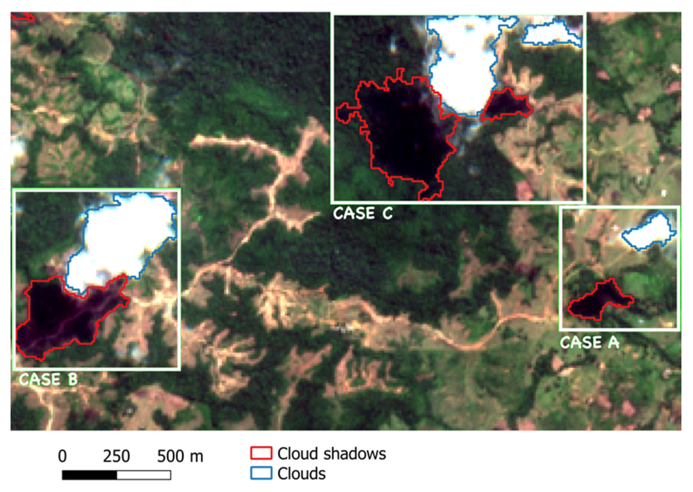
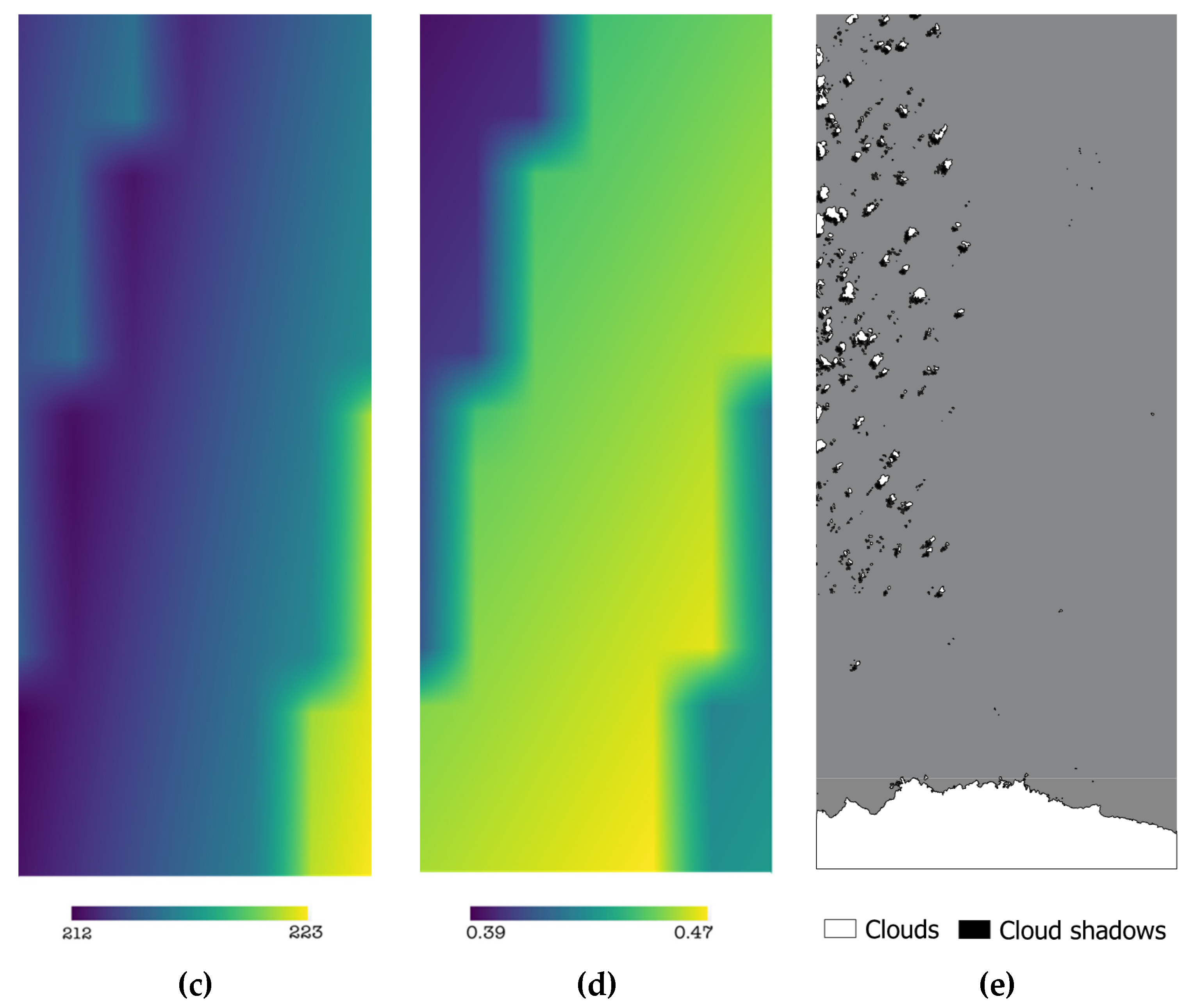
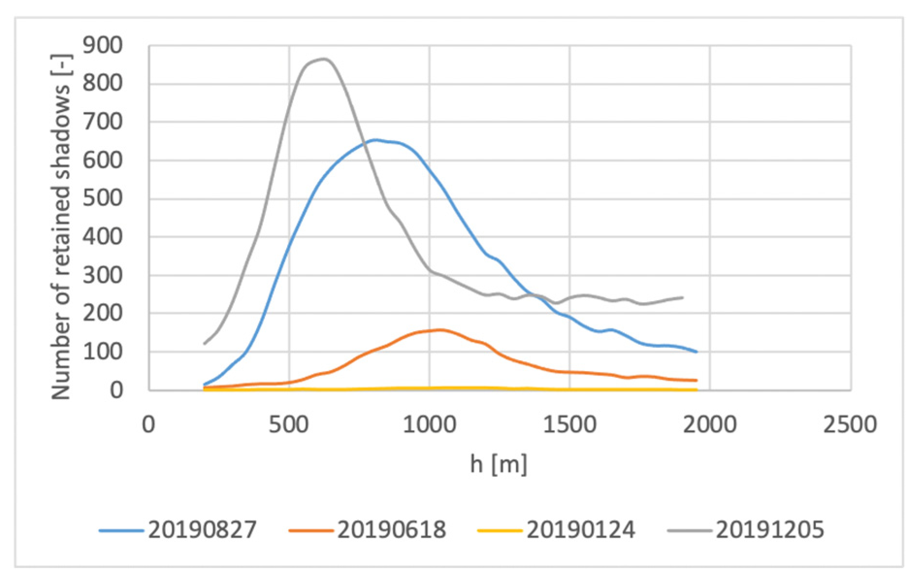
The approach illustrated an efficient improvement to cloud and cloud-shadow detection for Sentinel-2 using freely available tools. However, the approach also has its limitations. When a true shadow is located in a relatively dark area and is classified as a shadow along with its surroundings in one geometry, the entire geometry is retained as a shadow after the geometry-based improvement. Thus, those commissions cannot be excluded. Furthermore, the matching in the second iteration can result in commission errors in the shadows when candidate shadows are located in between a couple of matching cloud and shadow. Yet, all these potential drawbacks occur around areas where true cloud and shadow contamination exist, thus limiting the area of uncertainty in the results and leaving room for localized refinement of the methodology.
Another limitation of the presented methodology is that it is intended for relatively non-rugged terrain and relatively spatially homogeneous meteorological conditions where one representative hemp for cumulus clouds is considered. As such, additional considerations are needed for topography and potential micro-climates that can impact the cloud height with respect to the ground surface. However, the approach is scalable as it can be adjusted to allow the search for multiple representative hemp through considering local maxima for hemp when considering heterogenous areas. These aspects can be considered in the future when needed for other study areas.
As hemp is an empirical measure based on surface reflectance values, it is of great interest to analyze its correspondence to physical cloud characteristics. A future prospect of the work is to assess this measure’s link to cloud-top and cloud-base heights (thickness) at various scenarios of cloud-top ruggedness. This would require carrying out an analysis around areas where meteorological data are available or through the use of satellite data that allows for the extraction of cloud 3D geometry, such as geostationary data.

6. Conclusions

This paper addresses the important topic of cloud and cloud shadow detection over areas of Colombia where small-scale mining activities frequently occur. It presents a workflow of pixel-based classification followed by refinement of classes using solar-cloud-shadow-sensor geometry. The approach results in an improved detection of clouds and their shadows along with a reduction in commission errors. It makes use of freely available tools and does not require supplementary data on cloud-top or bottom heights nor cloud-top ruggedness. The geometry-based approach makes use of sun angles and sensor view angles available in Sentinel-2 metadata to identify potential directions of shadows for each pixel. For each cloud, this potential shadow direction is extracted using zonal statistics. An iterative approach is utilized for the exclusion of false positive shadows, given that cloud height is not available. In the first iteration, the focus is on low and dense clouds such as cumulus clouds where an empirical representative cloud height at the time of acquisition is obtained. A second iteration considers shadows and clouds not retained in the first iteration and considers higher cloud elevations. Non-retained shadows from the second iteration are relabeled as clear pixels and excluded from the cloud shadow mask. Compared to Sen2Cor, the semi-empirical model utilized for the atmospheric correction of Sentinel-2 data at the Copernicus Open Access Hub, the approach has shown a better detection of cloud and shadows. Furthermore, it has shown a reduction in the misclassification of mining and water pixels as clouds or shadows. Thus, this approach will be used to extract valid pixels of time-series of Sentinel-2 imagery over Antioquia for the development of an early warning system for sensitive areas that will be potentially affected by the uncontrolled sprawl of small-scale land-based alluvial mining.

Supplementary Materials

The following are available online at https://www.mdpi.com/2072-4292/13/4/736/s1, a .csv data file containing reference spectra used for the SVM classification to identify: Clouds, Cloud shadow, and Clear pixels. The data is extracted from a Sentinel-2 (S2B) L2A image acquired on 18 June 2019.

Author Contributions

Conceptualization, all authors; methodology, software, formal analysis, E.I., P.B., and J.J.; validation, E.I.; data curation, E.I. and L.L.; writing–original draft preparation, E.I.; writing–review and editing, all authors; visualization, E.I.; supervision, E.P., P.L., G.G.; funding acquisition, E.I., J.J., and E.P. All authors have read and agreed to the published version of the manuscript.

Funding

This research was funded by the Copernicus RawMatCop program, which is funded by EIT RawMaterials and the European Commission DG Internal Market, Industry, Entrepreneurship and SMEs (DG GROW). https://eitrawmaterials.eu/eit-rm-academy/rawmatcop/, as part of the scope of projects CopX: Geospatial Mining Transparency Through Copernicus and MapX, and EOAllert: Early-Warning to the Impacts of Alluvial Mining on Sensitive Areas Using Earth Observation (https://www.mapx.org/projects/eo-allert/)

Acknowledgments

The authors are thankful to several persons who made this work possible, especially: (a) at UNEP Geneva Office, David Jensen and Inga Peterson, who brought the collaborations in this paper to life, (b) at UNEP Bogota Office, Juan Bello, Juliana Ibarra, Silvio Lopez, and Ursula Jaramillo, for their continuous support in Colombia regarding field visits and stakeholder meetings, (c) the Secretary of Mines at El Bagre Rafael Sanchez, who helped us during data collection and for interviews of miners, and for his continuous support of any inquiries, (d) Julie Pirard for her great contributions to the graphics in this paper, and (e) André Muise, for his much-appreciated editing of the paper.

Conflicts of Interest

The authors declare no conflict of interest.

References

  1. Ministerio de Minas y Energía, C. Decreto 1666, Bogotá. Online. 2016. Available online: https://www.minenergia.gov.co/documents/10180/23517/37238-Decreto-1666-21Oct2016.pdf/17f4f90c-4481-47cd-a084-c7fa0319f9cf (accessed on 16 January 2021).
  2. Bustamante, N.; University of Queensland; Danoucaras, N.; McIntyre, N.; Martínez, J.C.D.; Baena, O.J.R.; De Colombia, U.N.; Mclntyre, N. Review of improving the water management for the informal gold mining in Colombia. Rev. Fac. Ing. Univ. Antioq. 2016, 79, 174–184. [Google Scholar] [CrossRef] [Green Version]
  3. Teschner, B.; Smith, N.M.; Borrillo-Hutter, T.; John, Z.Q.; Wong, T.E. How efficient are they really? A simple testing method of small-scale gold miners’ gravity separation systems. Miner. Eng. 2017, 105, 44–51. [Google Scholar] [CrossRef]
  4. Minambiente. Entra en Vigencia Prohibición del Mercurio en la Minería de oro en Colombia. 2018. Available online: https://www.minambiente.gov.co/index.php/noticias/4021-entra-en-vigencia-prohibicion-del-mercurio-en-la-mineria-de-oro (accessed on 16 February 2021).
  5. Ibrahim, E.; Lema, L.; Barnabé, P.; Lacroix, P.; Pirard, E. Small-scale surface mining of gold placers: Detection, mapping, and temporal analysis through the use of free satellite imagery. Int. J. Appl. Earth Obs. Geoinf. 2020, 93, 102194. [Google Scholar] [CrossRef]
  6. Diaz, F.A.; Katz, L.E.; Lawler, D.F. Mercury pollution in Colombia: Challenges to reduce the use of mercury in artisanal and small-scale gold mining in the light of the Minamata Convention. Water Int. 2020, 45, 730–745. [Google Scholar] [CrossRef]
  7. Rettberg, A.; Ortiz-Riomalo, J.F. Golden Opportunity, or a New Twist on the Resource–Conflict Relationship: Links Between the Drug Trade and Illegal Gold Mining in Colombia. World Dev. 2016, 84, 82–96. [Google Scholar] [CrossRef]
  8. Betancur-Corredor, B.; Loaiza-Usuga, J.C.; Denich, M.; Borgemeister, C. Gold mining as a potential driver of development in Colombia: Challenges and opportunities. J. Clean. Prod. 2018, 199, 538–553. [Google Scholar] [CrossRef]
  9. Portafolio. Producción Ilegal de Oro es Más del 70% del Mercado. 2019. Available online: https://www.portafolio.co/economia/produccion-ilegal-de-oro-es-mas-del-70-del-mercado-528760 (accessed on 11 December 2020).
  10. Hausermann, H.; Ferring, D.; Atosona, B.; Mentz, G.; Amankwah, R.; Chang, A.; Hartfield, K.; Effah, E.; Asuamah, G.Y.; Mansell, C.; et al. Land-grabbing, land-use transformation and social differentiation: Deconstructing “small-scale” in Ghana’s recent gold rush. World Dev. 2018, 108, 103–114. [Google Scholar] [CrossRef]
  11. UNODC. Alluvial Gold Exploitation: Evidences from Remote Sensing 2016; United Nations Office of Drugs and Crime: Vienna, Austria, 2018. [Google Scholar]
  12. Gallwey, J.; Robiati, C.; Coggan, J.; Vogt, D.; Eyre, M. A Sentinel-2 based multispectral convolutional neural network for detecting artisanal small-scale mining in Ghana: Applying deep learning to shallow mining. Remote. Sens. Environ. 2020, 248, 111970. [Google Scholar] [CrossRef]
  13. Zhang, R.; Sun, D.; Li, S.; Yu, Y. A stepwise cloud shadow detection approach combining geometry determination and SVM classification for MODIS data. Int. J. Remote. Sens. 2012, 34, 211–226. [Google Scholar] [CrossRef]
  14. Baetens, L.; Desjardins, C.; Hagolle, O. Validation of Copernicus Sentinel-2 Cloud Masks Obtained from MAJA, Sen2Cor, and FMask Processors Using Reference Cloud Masks Generated with a Supervised Active Learning Procedure. Remote. Sens. 2019, 11, 433. [Google Scholar] [CrossRef] [Green Version]
  15. Qiu, S.; Zhu, Z.; Woodcock, C.E. Cirrus clouds that adversely affect Landsat 8 images: What are they and how to detect them? Remote. Sens. Environ. 2020, 246, 111884. [Google Scholar] [CrossRef]
  16. Ackerman, S.A.; Strabala, K.I.; Menzel, W.P.; Frey, R.A.; Moeller, C.C.; Gumley, L.E. Discriminating clear sky from clouds with MODIS. J. Geophys. Res. Space Phys. 1998, 103, 32141–32157. [Google Scholar] [CrossRef]
  17. Zhu, Z.; Woodcock, C.E. Object-based cloud and cloud shadow detection in Landsat imagery. Remote. Sens. Environ. 2012, 118, 83–94. [Google Scholar] [CrossRef]
  18. Zhu, Z.; Wang, S.; Woodcock, C.E. Improvement and expansion of the Fmask algorithm: Cloud, cloud shadow, and snow detection for Landsats 4–7, 8, and Sentinel 2 images. Remote. Sens. Environ. 2015, 159, 269–277. [Google Scholar] [CrossRef]
  19. Louis, J.; Debaecker, V.; Pflug, B.; Main-Knorn, M.; Bieniarz, J.; Mueller-Wilm, U.; Cadau, E.; Gascon, F. Sentinel-2 SEN2COR: L2A processor for users. European Space Agency (Special Publication); SP-740; ESA SP: Paris, France, 2016; pp. 9–13. [Google Scholar]
  20. Hollstein, A.; Segl, K.; Guanter, L.; Brell, M.; Enesco, M. Ready-to-Use Methods for the Detection of Clouds, Cirrus, Snow, Shadow, Water and Clear Sky Pixels in Sentinel-2 MSI Images. Remote. Sens. 2016, 8, 666. [Google Scholar] [CrossRef] [Green Version]
  21. VITO. iCOR Plugin for SNAP Toolbox, Software User Manual, Version 1.0 Contents; Technical Report for VITO Remote Sensing Unit; VITO: Mol, Belgium, 2017. [Google Scholar]
  22. Baraldi, A.; Tiede, D. AutoCloud+, a “Universal” Physical and Statistical Model-Based 2D Spatial Topology-Preserving Software for Cloud/Cloud–Shadow Detection in Multi-Sensor Single-Date Earth Observation Multi-Spectral Imagery—Part 1: Systematic ESA EO Level 2 Product Generation at the Ground Segment as Broad Context. ISPRS Int. J. Geo-Inf. 2018, 7, 457. [Google Scholar] [CrossRef] [Green Version]
  23. Zhai, H.; Zhang, H.; Zhang, L.; Li, P. Cloud/shadow detection based on spectral indices for multi/hyperspectral optical remote sensing imagery. ISPRS J. Photogramm. Remote. Sens. 2018, 144, 235–253. [Google Scholar] [CrossRef]
  24. Nazarova, T.; Martin, P.; Giuliani, G. Monitoring Vegetation Change in the Presence of High Cloud Cover with Sentinel-2 in a Lowland Tropical Forest Region in Brazil. Remote. Sens. 2020, 12, 1829. [Google Scholar] [CrossRef]
  25. Sanchez, A.H.; Picoli, M.C.A.; Camara, G.; Andrade, P.R.; Chaves, M.E.D.; Lechler, S.; Soares, A.R.; Marujo, R.; Simões, R.E.O.; Ferreira, K.R.; et al. Comparison of Cloud Cover Detection Algorithms on Sentinel–2 Images of the Amazon Tropical Forest. Remote. Sens. 2020, 12, 1284. [Google Scholar] [CrossRef] [Green Version]
  26. Hagolle, O.; Huc, M.; Desjardins, C.; Auer, S.; Richter, R. MAJA ATBD Algorithm Theoretical Basis Document; Technical Report for CNES+CESBIO and DLR. 2017. Available online: https://www.theia-land.fr/wp-content-theia/uploads/sites/2/2018/12/atbd_maja_071217.pdf (accessed on 16 February 2021).
  27. Mateo-García, G.; Gómez-Chova, L.; Amorós-López, J.; Muñoz-Marí, J.; Camps-Valls, G. Multitemporal Cloud Masking in the Google Earth Engine. Remote. Sens. 2018, 10, 1079. [Google Scholar] [CrossRef] [Green Version]
  28. Wang, T.; Shi, J.; Husi, L.; Zhao, T.; Ji, D.; Xiong, C.; Gao, B. Effect of Solar-Cloud-Satellite Geometry on Land Surface Shortwave Radiation Derived from Remotely Sensed Data. Remote. Sens. 2017, 9, 690. [Google Scholar] [CrossRef] [Green Version]
  29. Luo, Y.; Trishchenko, A.; Khlopenkov, K. Developing clear-sky, cloud and cloud shadow mask for producing clear-sky composites at 250-meter spatial resolution for the seven MODIS land bands over Canada and North America. Remote. Sens. Environ. 2008, 112, 4167–4185. [Google Scholar] [CrossRef]
  30. Li, P.; Dong, L.; Xiao, H.; Xu, M. A cloud image detection method based on SVM vector machine. Neurocomputing 2015, 169, 34–42. [Google Scholar] [CrossRef]
  31. Torbick, N.; Chowdhury, D.; Salas, W.; Qi, J. Monitoring Rice Agriculture across Myanmar Using Time Series Sentinel-1 Assisted by Landsat-8 and PALSAR-2. Remote. Sens. 2017, 9, 119. [Google Scholar] [CrossRef] [Green Version]
  32. Talema, T.; Hailu, B.T. Mapping rice crop using sentinels (1 SAR and 2 MSI) images in tropical area: A case study in Fogera wereda, Ethiopia. Remote. Sens. Appl. Soc. Environ. 2020, 18, 100290. [Google Scholar] [CrossRef]
  33. Drusch, M.; Del Bello, U.; Carlier, S.; Colin, O.; Fernandez, V.; Gascon, F.; Hoersch, B.; Isola, C.; Laberinti, P.; Martimort, P.; et al. Sentinel-2: ESA’s Optical High-Resolution Mission for GMES Operational Services. Remote. Sens. Environ. 2012, 120, 25–36. [Google Scholar] [CrossRef]
  34. Müller-Wilm, U. Sentinel-2 MSI—Level 2A Products Algorithm Theoretical Basis Document. ref s2pad-atbd-0001 Issue 2.0; European Space Agency: Paris, France, 2012; 2p. [Google Scholar]
  35. ESA. European Space Agency Technical Guide: Cloud Masks (L1C). 2020. Available online: https://sentinel.esa.int/web/sentinel/technical-guides/sentinel-2-msi/level-1c/cloud-masks (accessed on 4 November 2020).
  36. ESA. European Space Agency Technical Guide: Cloud Masks (L2A). 2020. Available online: https://sentinel.esa.int/web/sentinel/technical-guides/sentinel-2-msi/level-2a/algorithm (accessed on 4 November 2020).
  37. Debouny, T.; Deprez, R.; Ibrahim, E.; Buydens, G.; Pirard, E. Assessing the discrepancy in open-source atmospheric correction of Sentinel-2 acquisitions for a tropical mining area in New Caledonia. In Proceedings of the Sixth International Conference on Remote Sensing and Geoinformation of the Environment (RSCy2018), Paphos, Cyprus, 26–29 March 2018; Volume 10773, p. 107730F. [Google Scholar]
  38. Sun, L.; Liu, X.; Yang, Y.; Chen, T.; Wang, Q.; Zhou, X. A cloud shadow detection method combined with cloud height iteration and spectral analysis for Landsat 8 OLI data. ISPRS J. Photogramm. Remote. Sens. 2018, 138, 193–207. [Google Scholar] [CrossRef]
  39. Lacroix, P.; Moser, F.; Benvenuti, A.; Piller, T.; Jensen, D.; Petersen, I.; Planque, M.; Ray, N. MapX: An open geospatial platform to manage, analyze and visualize data on natural resources and the environment. SoftwareX 2019, 9, 77–84. [Google Scholar] [CrossRef]
  40. Fisher, A. Cloud and Cloud-Shadow Detection in SPOT5 HRG Imagery with Automated Morphological Feature Extraction. Remote. Sens. 2014, 6, 776–800. [Google Scholar] [CrossRef] [Green Version]
  41. Huang, C.; Wylie, B.; Yang, L.; Homer, C.; Zylstra, G. Derivation of a tasselled cap transformation based on Landsat 7 at-satellite reflectance. Int. J. Remote. Sens. 2002, 23, 1741–1748. [Google Scholar] [CrossRef]
  42. Noi, P.T.; Kappas, M. Comparison of Random Forest, k-Nearest Neighbor, and Support Vector Machine Classifiers for Land Cover Classification Using Sentinel-2 Imagery. Sensors 2017, 18, 18. [Google Scholar] [CrossRef] [Green Version]
  43. Zafari, A.; Zurita-Milla, R.; Izquierdo-Verdiguier, E. Evaluating the Performance of a Random Forest Kernel for Land Cover Classification. Remote. Sens. 2019, 11, 575. [Google Scholar] [CrossRef] [Green Version]
  44. Pedregosa, F.; Varoquaux, G.; Gramfort, A.; Michel, V.; Thirion, B.; Grisel, O.; Blondel, M.; Prettenhofer, P.; Weiss, R.; Dubourg, V.; et al. Scikit-learn: Machine Learning in Python. J. Mach. Learn. Res. 2011, 12, 2825–2830. [Google Scholar]
  45. Mountrakis, G.; Im, J.; Ogole, C. Support vector machines in remote sensing: A review. ISPRS J. Photogramm. Remote. Sens. 2011, 66, 247–259. [Google Scholar] [CrossRef]
  46. Li, P.; Jiang, L.; Feng, Z. Cross-Comparison of Vegetation Indices Derived from Landsat-7 Enhanced Thematic Mapper Plus (ETM+) and Landsat-8 Operational Land Imager (OLI) Sensors. Remote. Sens. 2013, 6, 310–329. [Google Scholar] [CrossRef] [Green Version]
  47. Rokni, K.; Ahmad, A.; Selamat, A.; Hazini, S. Water Feature Extraction and Change Detection Using Multitemporal Landsat Imagery. Remote. Sens. 2014, 6, 4173–4189. [Google Scholar] [CrossRef] [Green Version]
  48. Du, Y.; Zhang, Y.; Ling, F.; Wang, Q.; Li, W.; Li, X. Water Bodies’ Mapping from Sentinel-2 Imagery with Modified Normalized Difference Water Index at 10-m Spatial Resolution Produced by Sharpening the SWIR Band. Remote. Sens. 2016, 8, 354. [Google Scholar] [CrossRef] [Green Version]
  49. Congedo, L. Semi-Automatic Classification Plugin Documentation Release 7.0.0.1. 2020. Available online: https://semiautomaticclassificationmanual.readthedocs.io/fr/latest/introduction.html (accessed on 16 February 2021).
  50. ESA. European Space Agency Technical Guide: Sentinel-2 Orbit. 2020. Available online: https://sentinel.esa.int/web/sentinel/missions/sentinel-2/satellite-description/orbit (accessed on 4 November 2020).
  51. Le Hégarat-Mascle, S.; André, C. Use of Markov Random Fields for automatic cloud/shadow detection on high resolution optical images. ISPRS J. Photogramm. Remote. Sens. 2009, 64, 351–366. [Google Scholar] [CrossRef]
  52. Hughes, M.J.; Hayes, D.J. Automated Detection of Cloud and Cloud Shadow in Single-Date Landsat Imagery Using Neural Networks and Spatial Post-Processing. Remote. Sens. 2014, 6, 4907–4926. [Google Scholar] [CrossRef] [Green Version]
  53. Candra, D.S.; Phinn, S.; Scarth, P. Automated Cloud and Cloud-Shadow Masking for Landsat 8 Using Multitemporal Images in a Variety of Environments. Remote. Sens. 2019, 11, 2060. [Google Scholar] [CrossRef] [Green Version]
  54. Johnson, R.H.; Rickenbach, T.M.; Rutledge, S.A.; Ciesielski, P.E.; Schubert, W.H. Trimodal Characteristics of Tropical Convection. J. Clim. 1999, 12, 2397–2418. [Google Scholar] [CrossRef]
  55. Duarte, R.P.; Gomes, A.J. Real-time simulation of cumulus clouds through SkewT/LogP diagrams. Comput. Graph. 2017, 67, 103–114. [Google Scholar] [CrossRef]
  56. Pancel, L.; Köhl, M. Tropical Forestry Handbook; Springer: Berlin/Heidelberg, Germany, 2016. [Google Scholar]
  57. FAA. Pilot’s Handbook of Aeronautical Knowledge, Chapter 12: Weather Theory. 2020. Available online: https://www.faa.gov/ (accessed on 16 February 2021).
  58. Gillies, S. Rasterio: Geospatial Raster I/O for Python Programmers. 2018. Available online: https://github.com/mapbox/rasterio (accessed on 16 February 2021).
  59. Perry, M.T. Rasterstats. 2017. Available online: https://github.com/perrygeo/python-rasterstats/blob/master/docs/manual.rst (accessed on 4 November 2020).
  60. Gillies, S. Shapely: Manipulation and Analysis of Geometric Objects. 2007. Available online: https://github.com/Toblerity/Shapely (accessed on 16 February 2021).
  61. Jordahl, K.; den Bossche, J.V.; Wasserman, J.; McBride, J.; Gerard, J.; Tratner, J.; Perry, M.; Farmer, C.; Cochran, M.; Gillies, S.; et al. Geopandas/Geopandas: V0.4.1. 2019. Available online: https://https://zenodo.org/record/2585849#.YC3BB3kRWUk (accessed on 16 February 2021).
  62. Schläpfer, D.; Richter, R.; Reinartz, P. Elevation-Dependent Removal of Cirrus Clouds in Satellite Imagery. Remote. Sens. 2020, 12, 494. [Google Scholar] [CrossRef] [Green Version]
  63. ESA. Recommendations of the Workshop Uncertainty in Remote Sensing. 2017. Available online: https://earth.esa.int/eogateway/events/workshop-on-uncertainties-in-remote-sensing (accessed on 16 February 2021).
  64. Benner, T.C.; Curry, J.A. Characteristics of small tropical cumulus clouds and their impact on the environment. J. Geophys. Res. Space Phys. 1998, 103, 28753–28767. [Google Scholar] [CrossRef]
  65. Zekoll, V.; Main-Knorn, M.; Alonso, K.; Louis, J.; Frantz, D.; Richter, R.; Pflug, B. Comparison of Masking Algorithms for Sentinel-2 Imagery. Remote. Sens. 2021, 13, 137. [Google Scholar] [CrossRef]
Figure 1. An overview of the study area (a) The location and extent of the study area in Colombia and Antioquia; (b) Sentinel-2 (S2B) RGB image (18 June 2019) of the study area with the white oval locating the pilot site (around the town of El Bagre at latitude 7°36’17.88’’N and longitude 74°48’32.32’’W) that is used for the validation of the methodology, (c) DEM SRTM.
Remotesensing 13 00736 g001aRemotesensing 13 00736 g001b
Figure 2. (a) Mean temperature and (b) Seasonal temperature variability of the study area (boundary shown as black rectangle) and its surroundings (Antioquia’s administrative boundaries shown as dotted polygon). The data source is WorldClim (30 arc-second resolution), a global gridded historical dataset (1960 to 1991) that has been vital for various environmental studies. The data were obtained through Google Earth Engine (https://earthengine.google.com/:collection WORLDCLIM-V1-BIO).
Remotesensing 13 00736 g002
Figure 3. An illustration of reflectance spectra of a selection of cloud and cloud-shadow pixels along with water and bare soil mining pixels; (a) A selection of the region of interest on an RGB Sentinel-2 (S2B) (18 June 2019); (b) Mean spectra ± 1 standard deviation of selected regions plotted using the Semi-Automated Classification plugin (SCP) [49].
Remotesensing 13 00736 g003
Figure 4. An illustration of cloud and cloud shadow geometry.
Remotesensing 13 00736 g004
Figure 5. An overview of the steps in improving classified cloud shadows for the reduction of false positives. Specific python libraries and functions are indicated in blue where applicable.
Remotesensing 13 00736 g005
Figure 6. Examples of clouds and their shadows illustrating their possible separation and adjacency using a Sentinel-2 image of the study area.
Remotesensing 13 00736 g006
Figure 7. An illustration of the cloud and cloud-shadow detection procedure: (a) RGB view of an image acquired on 27 August 2018; (b) the results of the supervised classification of the Support-Vector-Machine SVM) with detected clouds (white) and cloud shadows (black stripes); (c) the retained cloud shadows of low dense clouds detected by the first iteration; (d) the retained and excluded cloud shadows by the end of the second iteration where the excluded clouds are relabeled as clear pixels.
Remotesensing 13 00736 g007
Figure 8. The pilot site and reference data (a) Reference locations in the pilot site shown on band 2 of Sentinel-2 image acquired on 18 June 2019 (b) Photo of a mining site in the pilot area.
Remotesensing 13 00736 g008
Figure 9. (a) Sun and (b) sensor viewing angles for the study area of the Sentinel-2 image acquired on 18 June 2019.
Remotesensing 13 00736 g009
Figure 10. Cloud and cloud shadow detection for the sentinel-2 image acquired on 18 June 2019 (a) RGB view of the image over the study area, (b) SVM classification results of clouds and cloud shadows, (c) φa [degrees], (d) d/h [–], (e) geometry-based improved cloud shadows.
Remotesensing 13 00736 g010aRemotesensing 13 00736 g010b
Figure 11. h values tested during the first iteration and the corresponding retained shadows. The maxima represent the hemp values in Table 4.
Remotesensing 13 00736 g011
Figure 12. Sentinel-2 RGB view of the three images and their corresponding detected dense clouds, and cloud shadows, along with cirrus cloud provided by Sen2Cor (a) 24 January 2019, (b) 27 August 2019, and (c) 5 December 2019.
Remotesensing 13 00736 g012
Figure 13. Sentinel-2 18 June 2019 close-up (a) RGB view, (b) cloud and cloud-shadow detection by the current approach, (c) cloud and cloud-shadow detection by Sen2Cor.
Remotesensing 13 00736 g013
Figure 14. True positives of visually detected using the current approach compared to Sen2Cor (a) dense clouds (512 and 581 reference pixels as indicated in the first column) and (b) shadows (470 and 496 reference pixels as indicated in the first column).
Remotesensing 13 00736 g014
Figure 15. Specificity in the correct negative identification with respect to dense clouds and shadows for the reference date of the pilot site (a) mining areas (b) water bodies.
Remotesensing 13 00736 g015
Table 1. Wavelengths and bandwidths of the two MSI sensors on board the Sentinel-2 twin satellites.
BandSpatial Resolution (m)S2AS2B
Central Wavelength (nm)Bandwidth (nm)Central Wavelength (nm)Bandwidth (nm)
B160442.721442.221
B210492.466492.166
B310559.83655936
B410664.631664.931
B520704.115703.816
B620740.515739.115
B720782.820779.720
B810832.8106832.9106
B8a20864.72186422
B960945.120943.221
B10601373.5311376.930
B11201613.7911610.494
B12202202.41752185.7185
Table 2. Overview of reference spectra.
ClassNumber of Reference Spectra
Clouds18,547
Cloud Shadows17,610
Clear Pixels18,273
Table 3. Optimal SVM Kernel parameters and classification accuracy.
FeaturesKernelCGammaPr
B1 to B9 and B11 to B12RBF10010.995 ±0.008
B1 to B9 and B11 to B12, NDVIRBF20010.995 ±0.008
B1 to B9 and B11 to B12, MNDWIRBF5010.995 ±0.009
B1 to B9 and B11 to B12, NDVI, MNDWIRBF10010.995 ±0.008
B1, B9, NDVI, and MNDWIRBF110.976 ±0.005
Table 4. Parameters of potential cloud-shadow direction and location.
DatePlatformφa [degrees]d/h [-]hemp [m]
24 January 2019S2A321–3280.61–0.681050
18 June 2019S2B212-2230.39-0.471050
27 August 2019S2B248–2600.25–0.33800
5 December 2019S2B332–3400.60–0.67600
Table 5. Estimated height of low dense clouds using meteorological data at the Los Garzones International Airport Station.
Date TimeTs [degrees] Tdew [degrees] hmet [m]
24 January 201910:29 a.m.30.824.2806
18 June 201910:29 a.m.33.227.7671
27 August 201910:00 a.m.32.227.2610
5 December 201909:53 a.m.29.627.2294
Table 6. Overview of clear reference mining bare soil pixels (number of total negatives, Neg) in each image and the number of false positives (F), (prob. is an abbreviation of probability).
Neg Mining PixelsDateF Sen2CorF Current Approach
ShadowHigh Prob.Medium Prob.ShadowClouds
291624 January 2019061200
294718 June 20190203000
266727 August 2019001100
29165 December 201900300
Table 7. Overview of clear reference water pixels (number of total negatives, Neg) in each image and the number of false positives (F), (prob. is an abbreviation of probability)}.
Neg Water PixelsDateF Sen2CorF Current Approach
ShadowHigh Prob.Medium Prob.ShadowClouds
294724 January 2019031400
294718 June 2019007000
283527 August 20192004351700
29475 December 201912802900
Publisher’s Note: MDPI stays neutral with regard to jurisdictional claims in published maps and institutional affiliations.

