Potential of P-Band SAR Tomography in Forest Type Classification

Abstract

Forest type classification using spaceborne remote sensing is a challenge. Low-frequency Synthetic Aperture Radar (SAR) signals (i.e., P-band, ∼0.69 m wavelength) are needed to penetrate a thick vegetation layer. However, this measurement alone does not guarantee a good performance in forest classification tasks. SAR tomography, a technique employing multiple acquisitions over the same areas to form a three-dimensional image, has been demonstrated to improve SAR’s capability in many applications. Our study shows the potential value of SAR tomography acquisitions to improve forest classification. By using P-band tomographic SAR data from the German Aerospace Center F-SAR sensor during the AfriSAR campaign in February 2016, the vertical profiles of five different forest types at a tropical forest site in Mondah, Gabon (South Africa) were analyzed and exploited for the classification task. We demonstrated that the high sensitivity of SAR tomography to forest vertical structure enables the improvement of classification performance by up to 33%. Interestingly, by using the standard Random Forest technique, we found that the ground (i.e., at 5–10 m) and volume layers (i.e., 20–40 m) play an important role in identifying the forest type. Together, these results suggested the promise of the TomoSAR technique for mapping forest types with high accuracy in tropical areas and could provide strong support for the next Earth Explorer BIOMASS spaceborne mission which will collect P-band tomographic SAR data.

1. Introduction

The world’s forests cover a total area of 4.06 billion hectares, comprising around 31% of the total land surface of the Earth [1]. They play an important role in maintaining biological interactions (i.e., biodiversity) and moderating the concentration of atmospheric greenhouse gases and therefore the climate [2]. However, these forests are currently decreased and degraded due to human activities [3]. This leads to accelerated soil erosion and a reduction in forest carbon stocks. To reduce forest carbon emissions, there is an increasing need to assess the distribution of forest resources [4,5,6]. For countries planning to participate in the Reducing Emissions from Deforestation and Degradation (REDD) program, quantifying forest biomass and forest areas is essential. These countries will benefit from incentives (e.g., monetary compensation) offered by REDD to preserve their forestland in the interest of reducing carbon emissions and thereby mitigating climate change [7].

Earth observation—based either on airborne or satellite systems—is important for forest monitoring as demonstrated by many published works in the literature [4,5,6,8,9,10]. Remotely sensed imagery has become an important data source mainly because remote sensing techniques can provide a synoptic view, allowing the production of mapping from local to global scales. Thanks to the rapid development of remote sensing technologies, the mapping of forest ecosystem biomass stocks has been done using a range of new and more precise methods. Nevertheless, despite many advances in the research and development of new applications, important limitations on the accurate estimation and mapping of biomass still exist [4,5]. New technologies are urgently needed to efficiently provide more precise data that will enable the observation and monitoring of forests at large geographical scales.

BIOMASS, the next ESA Earth Explorer Core Mission, will deliver accurate global maps of the amount of carbon stored in the world’s forests and how this changes over time as its primary strategic goal [10,11,12]. The BIOMASS satellite, planned for a 2022/2023 launch date, will achieve the goal of the global mapping of forest biomass by using a fully polarimetric Synthetic Aperture Radar (SAR). BIOMASS will be unique among satellites because it will collect, for the first time from space, SAR tomography data at the P-band (at 435 MHz, with a 69 cm wavelength and 25 m spatial resolution). The transmitted wave, owing to its low frequency, will be able not only to penetrate the vegetation down to the ground [13] but also to obtain the vertical distribution of vegetation in dense multi-layered tropical forests [11]. The operation of the BIOMASS satellite will comprise two different observation phases: the tomographic phase and the interferometric phase. The revisit time during the tomographic phase is planned to be 3 days to minimize temporal decorrelation in three-dimensional reconstruction, after which, in the interferometric phase, it will be increased to 17 days [14]. During the first year of its lifetime, the BIOMASS satellite will collect tomographic data and generate a map at a 200 m resolution of the global forest biomass. These maps will then be updated every six months during the interferometric phase for four years. The goal of the BIOMASS mission will be to provide biomass maps with a 20% acceptable error at a resolution of 4 ha [10,11,12]. For the acquisition of data to image vertical forest structure by employing SAR tomography (TomoSAR), the satellite’s orbit will be modified and designed in a new way. It will gather multiple acquisitions over the same sites from slightly different orbital positions [11]. In consequence, the BIOMASS satellite will be able to provide information on vertical forest structure using P-band TomoSAR from space.

SAR tomography is an emerging technology used to image the three-dimensional (3D) structure of illuminated media [9,15,16,17,18]. TomoSAR exploits the key feature of microwaves to penetrate into vegetation, providing the possibility to see features that are hidden to optical and hyperspectral systems. In contrast to optical and hyperspectral imaging, TomoSAR measurements provide significantly higher sensitivity to the vertical arrangement of forest elements due to the ability to penetrate through the vegetation layer and interact with forest structure components at different heights [16,19,20]. Although LiDAR systems can measure precise vertical forest structure, TomoSAR has the advantage of a higher penetration ability through clouds/vegetation and wide-swath imaging capacities that can provide information at a large scale at high temporal and spatial resolutions [10,11,12]. P-band TomoSAR tomography has been reported as a unique tool to survey and monitor tropical forests (e.g., forest biomass, canopy height, and sub-canopy terrain topography) [9,19]. The open question now is how to exploit TomoSAR to better characterize forest structure—specifically, how can TomoSAR products help produce a new product such as ecological forest types? In this work, we aim to address this question.

For classification tasks, as shown in the literature regarding remote sensing, supervised machine learning methods are a natural choice [21,22]. In these methods, training sets are used to train a certain algorithm and then classify pixels with an unknown identity. In practice, there is a trade-off between the performances and interpretability (and computation time) of the results [23]. Recently, the developments have focused on active learning and semisupervised learning approaches [24,25,26] for the small amount of trained data, whereas Deep Learning techniques (e.g., convolutional [27] and recurrent [28] neural networks) are exploited when massive trained data are available [29,30]. In remote sensing, most works are based on the standard algorithms such as Support Vector Machine and Random Forest [31]. In this paper, we prefer the Random Forest approach as it enables us to evaluate feature contributions, offering great interpretability of the results.

The rest of the article is structured as follows: the forest study site and the associated data are introduced in Section 2; Section 3 describes the TomoSAR processing and Random Forest for forest type classification; the experimental results are reported in Section 4; and finally, Section 5 provides the associated discussion and conclusions.

2. Materials

2.1. Study Site

The study region is in the Mondah tropical forest area in Gabon, Africa. The area is located 25 km from Libreville airport. This forest includes different biomass levels and growth stages. It is a relatively young forest with highly variable density and shows some degradation due to its proximity to a population center [32]. The Mondah area is characterized by more levels of diversity than other forest sites in Gabon. We limited our study area to this forest to demonstrate our approach. Figure 1 shows the geographic location of the Mondah tropical forest area, corresponding to a coverage of about 6.7 km × 8 km (latitude–longitude). The tomographic SAR data and the reference data are reported in Section 2.2 and Section 2.3, respectively.

2.2. Tomographic P-Band SAR Data

In the framework of ESA’s future BIOMASS satellite mission, the AfriSAR campaign was designed and carried out to support development and assessment algorithm activities.

The Mondah forest area was studied by two flights in 2015 and 2016 [33,34]. The campaign was shared between ONERA (dry season, July 2015) and the German Aerospace Center (DLR) (wet season, February 2016). Campaign SAR data can be found at the ESA EOPI portal (http://eopi.esa.int). In this paper, we focused on the DLR F-SAR tomographic data sets, which consisted of 11 fully polarimetric Single Look Complex (SLC) images at P-band (reference track 502 and ID from 202 to 212). The tomographic baseline is shifted vertically over the reference track, resulting in the 160 m baseline aperture. The covered area is approximately 5 km × 8 km (range-azimuth). The detailed information is reported in

Table 1. Description of the F-SAR system configuration for P-band tomographic acquisition parameters in Mondah.

Acquisition Parameters
Baseline configuration	vertical
Baseline aperture	160 (m)
Wavelength	0.689 (m)
Angle range	25–60 (deg)
Range Bandwidth	50 (MHz)
Azimuth resolution	1.5 (m)
Range resolution	2.25 (m)
Vertical resolution	10.0 (m)
Azimuth pixel size	0.81 (m)
Range pixel size	1.20 (m)
Flight averaged altitude	6096 (m)

.

2.3. Reference Data

For this investigation, we chose five observed forest type classes based on their diversity: (1) very low; (2) low; (3) moderate; (4) high; and (5) very high. The level of diversity can be associated with different spatial patterns of the canopy (and biomass). The signature of each class is reported in

Table 2. Description of the forest type class in Mondah.

ID	Forest Class	Key Signatures
(1)	Very low degraded vegetation	Very close to the main roads, few trees within, partly open areas
(2)	Forest with low diversity	Close to the main roads, monodominant trees, coarse pattern
(3)	Forest with moderate diversity	A mix of coarse and intermediate patterns, moderately dense forest areas
(4)	Forest with high diversity	A mix of intermediate and fine patterns, densely forested areas
(5)	Forest with very high diversity	Fine pattern, very densely forested areas

. Figure 1 shows the position of plots. For each class, 30 plots of 100 m × 100 m (1 ha) were defined manually, based on a careful visual interpretation of the layer high-resolution World Imagery of ArcGIS online (accessed in July 2020). In total, 150 reference plots were selected based on their flat topography and within-plot homogeneity. The plot data can be accessed in the supplement as a shapefile in the WGS84 UTM 32N coordination system. A zoomed version of the 12 sample plots with the World Imagery background is shown in Figure 2.

3. Methods

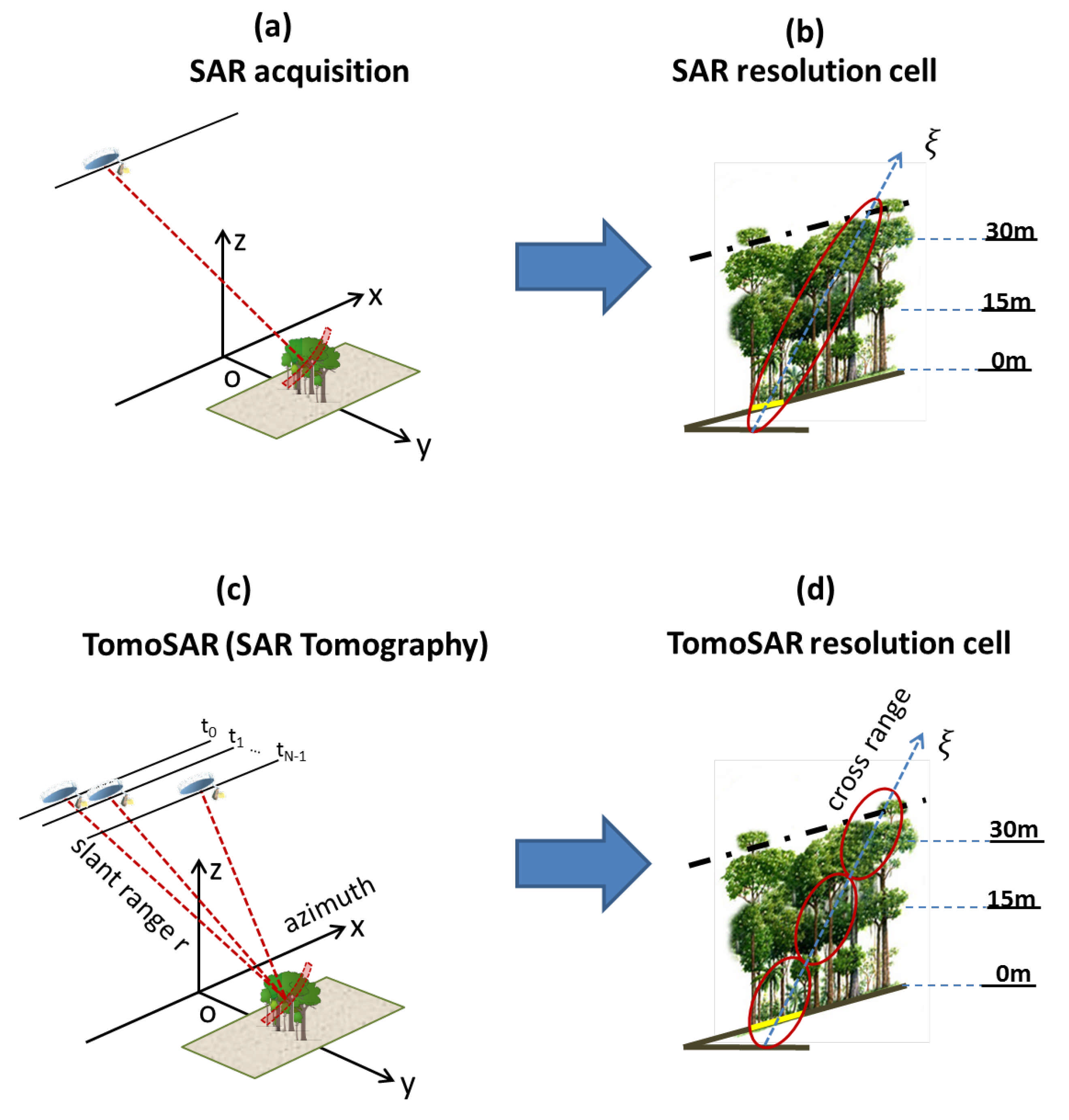
3.1. SAR Tomographic Imaging

If the radar wavelength is long enough to penetrate the canopy [13], multiple SAR acquisitions with a slightly different look angle over the same area can allow us to quantify the three dimensions of the forest reflectivity. In Figure 3a,c, the acquisitions from a traditional SAR and TomoSAR are shown, respectively. Unlike a traditional SAR (which refers to only one SAR scene), the principle of TomoSAR is to employ multiple flight tracks that are nearly parallel to each other to form a 3D image. Let us consider multi-baseline data of SAR images acquired by a carefully flying sensor along N parallel tracks. We denote $I_n$$\left(r,x\right)$ as the pixel at the slant range $\left(r\right)$, azimuth location $\left(x\right)$ in the n image. The azimuth axis x is defined by the direction of the aircraft platform, whereas the slant range is the distance line-of-sight (LOS) linking the SAR’s sensor to targets on the ground, as shown in Figure 3c. Let us assume that each image within the multi-baseline dataset has been coregistered and resampled on a common grid (i.e., the reference track), and that phase components due to terrain topography and platform motion have been compensated; thus, the multi-baseline SAR model can be written as [15]

$$I_n\left(r,x\right)=\int S\left(\xi ,r,x\right)exp\left(j\frac{4\pi }{\lambda r}{b}_n\xi \right)d\xi$$

(1)

where $\xi$ is the cross-range coordinate, defined by the direction orthogonal to the LOS and the azimuth coordinate; $b_n$ is the normal baseline relative to the n image with respect to the reference image; $\lambda$ is the carrier wavelength; and $S\left(\xi ,r,x\right)$ is the average scene complex reflectivity within the slant range, azimuth and cross-range resolution cell, as shown in Figure 3d. We note that there is a direct link between the SAR scene and the geometric configuration. In detail, the distribution of the SAR scene reflectivity in the cross-range direction and the multi-baseline SAR data form a Fourier pair (see Equation (1)). Consequently, the cross-range distribution of the scene complex reflectivity can be reconstructed by taking the Fourier Transform as follows [19]:

$$\widehat{S}(\xi ,r,x)=\sum _{n=1}^N{I}_n\left(r,x\right)exp\left(-j\frac{4\pi }{\lambda r}{b}_n\xi \right)$$

(2)

As a result, at each range and azimuth location, we are able to retrieve the cross-range distribution of the SAR scene reflectivity. In other words, TomoSAR processing allows us to provide full 3D imaging capabilities. The transformation from the cross-range axis $S(\xi ,r,x)$ to height direction $S(z,r,x)$ can be obtained by dividing the cosine of the local incidence angle.

The outline theoretical model for tomographic analysis is possible when there are no disturbances in the propagating signal. In fact, prior to this focusing, the phase calibration procedure of the TomoSAR data should be taken into account in order to compensate for the phase residuals that can influence the 3D focusing. These phase disturbances are mostly from atmospheric propagation delays and uncompensated platform motions. In this paper, the phase screen compensation is carried out by using the Double Localization iterative procedure described in detail in [17].

3.2. Random Forest

There are many supervised machine learning approaches that are currently available for classification tasks. In this work, we consider the Random Forest approach to study the performance of TomoSAR for forest classification. The motivation for this choice is mainly that (1) it enables us to evaluate the feature contributions in its procedure, and (2) it also is the most popular method in remote sensing and remains competitive with respect to other approaches in many applications and scenarios. For the sake of completion, we provide a brief introduction of this method as below.

The Random Forest algorithm is well documented and well demonstrated in the literature [35,36]. In fact, the renown of Random Forest is due to its ability to yield high-quality mappings with a very efficient and fast computation in comparison to other state-of-the-art classifiers. The classifier’s core algorithm relies on aggregating the results of an ensemble of simpler decision tree classifiers. In other words, it is a meta-estimator that fits several decision tree classifiers on various subsamples of the dataset and uses averaging to improve the predictive accuracy and control over-fitting [35]. Tree construction can be stopped when a maximum depth is reached or when the number of samples on the node is less than a minimum sample threshold. This is the main constraint to increase efficient calculation and to reduce the computational complexity of the algorithm and the correlation between subsamples.

During the tree construction process, features are evaluated and weighted. In this way, each feature contribution can be assessed and selected. Indeed, feature selection is preferable to feature transformation because the original units and meanings of features are more important in many applications. In practice, by selecting the most important features, the processing can be carried out on the reduced feature set. In other words, feature selection can be used for many dimension reduction applications, typically in massive hyperspectral data.

We compare classification results from non-tomographic (i.e., traditional SAR) and tomographic data. For the traditional SAR image, we use the original data from the reference track 502. We have three feature inputs—HH, HV, and VV (where H is horizontal and V is vertical)—as polarizations for the classification. For tomographic layers, with each polarization, we exploit nine layers at 5 m intervals (i.e., from 0 m to 40 m), resulting in 27 feature inputs.

For the Random Forest model, the parameters are optimized by a grid search to get the best performance. As a result, we set the number of parameters to be used at each node split at 5 and a maximum tree depth of 7. We use the Python implementation provided by the Scikit-learn library [37].

4. Results

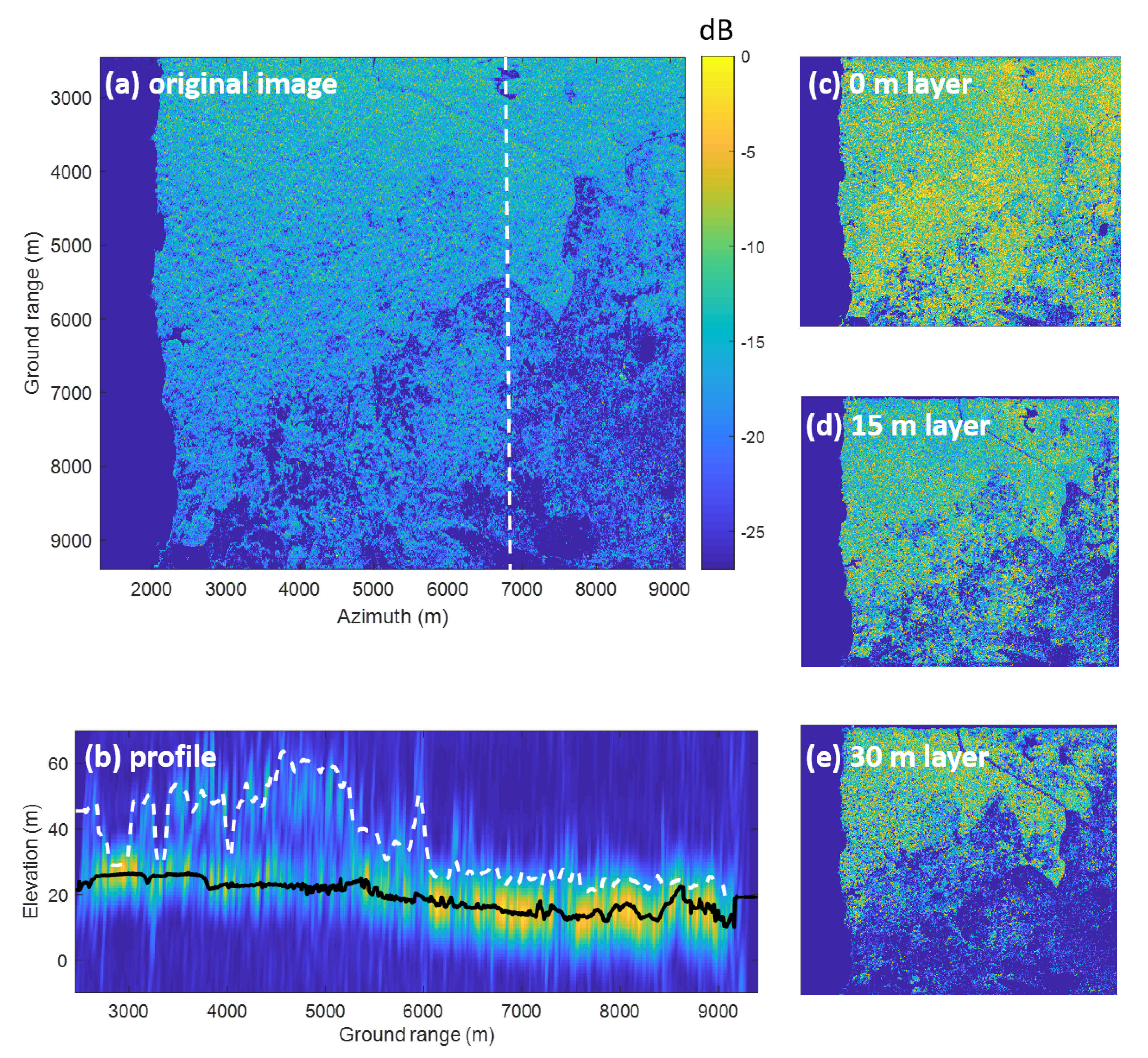
4.1. Tomographic Multi-Layer Forest Imaging

By exploiting the ensemble of all flight lines in TomoSAR processing, the multi-baseline SAR data can be transformed into a new multi-layer composite SAR image. Each layer of this new stack is characterized by the contribution of the scene reflectively at a certain height above ground level (see, for example, Figure 4c–e). For simplicity, each image within the multi-layer data stack is referred to the associated height (e.g., 15-m layer, 30-m layer...), in which the 0 m layer corresponds to the ground layer.

TomoSAR products offer a convenient way to observe the forest’s vertical structure at a local scale by taking a profile which is the vertical section of the multi-layer data stack. In Figure 4b, a tomographic vertical section was obtained by processing HV polarization. We can observe that, although the forest height is about 40 m, there are relevant contributions from the ground level. However, beneath the forest, such ground contributions are likely to be smaller than that of the vegetation layers. Thus, P-band TomoSAR allows us to capture the 3D forest scene due to its capability to penetrate to the ground level.

4.2. Backscatter versus Forest Class

The variation of backscatter with respect to forest type classes is analyzed as a function of height and polarization.

Figure 5 reports the vertical profile of five different forest classes, showing the behavior of HH, HV, and VV backscattering coefficients. As expected, it can be observed that the HH and VV backscatter values are higher than those of the HV polarization. In classes (4) and (5), the most concentrated intensity location in the vertical direction is around 30 m; that is, much higher than those from classes (1), (2), and (3). The dynamic ranges of HH, HV, and VV backscatter are very similar, in which the narrowest range is at 0 m (about 3 dB) and the widest one is at 35 m (about 18 dB) (see also

Table A1. The average and standard deviation of the five forest classes for tomographic layers.

Polarization	Layer	Forest Class Intensity (dB)
		1	2	3	4	5
	0 m	$-2.8\pm 5.1$	$-0.9\pm 2.2$	$-1.4\pm 2.9$	$-1.7\pm 2.9$	$-2.8\pm 2.9$
	5 m	$-3.5\pm 5.0$	$-0.9\pm 2.1$	$-2\pm 2.8$	$-2.3\pm 3$	$-3.9\pm 2.4$
	10 m	$-6.7\pm 4.6$	$-2.4\pm 1.8$	$-3.5\pm 2.3$	$-4.9\pm 2.7$	$-6.1\pm 2.2$
	15 m	$-13\pm 4.5$	$-4.4\pm 2.0$	$-4.4\pm 2.1$	$-6.1\pm 2.2$	$-7\pm 1.9$
HH	20 m	$-18.6\pm 3.7$	$-6.5\pm 2.5$	$-4.3\pm 2.3$	$-5.0\pm 2.2$	$-6.5\pm 2.1$
	25 m	$-19.7\pm 5.0$	$-8.8\pm 2.6$	$-5.3\pm 2.6$	$-3.8\pm 2.0$	$-5.3\pm 2.0$
	30 m	$-20.9\pm 4.1$	$-12.0\pm 2.7$	$-7.3\pm 3.0$	$-3.1\pm 2.2$	$-3.8\pm 2.1$
	35 m	$-21.2\pm 4.7$	$-14.4\pm 2.9$	$-9.4\pm 3.5$	$-4.2\pm 2.7$	$-3.0\pm 2.3$
	40 m	$-20.3\pm 5.6$	$-15\pm 2.7$	$-11.8\pm 3.4$	$-7.0\pm 3.5$	$-3.6\pm 2.4$
	0 m	$-10.8\pm 5.4$	$-6.6\pm 1.7$	$-8.2\pm 2.0$	$-8.1\pm 2.1$	$-10.3\pm 2.7$
	5 m	$-11.4\pm 5.2$	$-6.1\pm 1.7$	$-8.5\pm 1.9$	$-8.7\pm 2.0$	$-10.9\pm 2.3$
	10 m	$-14.4\pm 4.8$	$-6.9\pm 1.7$	$-9.4\pm 2.1$	$-10.7\pm 2.0$	$-12.2\pm 2.0$
	15 m	$-20.3\pm 5.2$	$-8.6\pm 2.1$	$-9.3\pm 1.9$	$-10.6\pm 2.3$	$-12.5\pm 1.5$
HV	20 m	$-25.1\pm 4.3$	$-10.7\pm 2.1$	$-9.1\pm 2.3$	$-9.1\pm 2$	$-11.5\pm 1.9$
	25 m	$-26.5\pm 3.5$	$-13.4\pm 2.3$	$-9.9\pm 2.6$	$-8.4\pm 2.3$	$-9.9\pm 2.2$
	30 m	$-27.3\pm 3.5$	$-16.4\pm 2.5$	$-11.9\pm 2.4$	$-8.1\pm 2.4$	$-8.4\pm 2.3$
	35 m	$-27.5\pm 4.4$	$-18.6\pm 2.6$	$-14.7\pm 2.7$	$-9.4\pm 2.3$	$-7.6\pm 2.2$
	40 m	$-26.4\pm 4.7$	$-19.8\pm 2.3$	$-17.5\pm 3.4$	$-12.2\pm 3.0$	$-7.9\pm 2.3$
	0 m	$-3.7\pm 4.1$	$-1.8\pm 2.2$	$-3.3\pm 2.4$	$-3.6\pm 2.4$	$-5.3\pm 3.1$
	5 m	$-4.3\pm 4.0$	$-1.4\pm 2.0$	$-3.2\pm 2.0$	$-4.2\pm 2.6$	$-6.1\pm 2.6$
	10 m	$-7.3\pm 3.8$	$-2.0\pm 1.6$	$-4.2\pm 1.9$	$-6\pm 2$	$-7.7\pm 2.0$
	15 m	$-13.6\pm 4.4$	$-3.6\pm 2.0$	$-4.6\pm 2.0$	$-6.2\pm 2.1$	$-7.8\pm 1.5$
VV	20 m	$-19.1\pm 3.9$	$-5.4\pm 2.8$	$-4.3\pm 2.3$	$-4.9\pm 2.1$	$-6.6\pm 1.7$
	25 m	$-20.7\pm 4.1$	$-7.8\pm 3.4$	$-5.0\pm 2.7$	$-3.7\pm 2.1$	$-5.1\pm 2.2$
	30 m	$-21.2\pm 3.7$	$-10.7\pm 3$	$-6.6\pm 3.1$	$-3.1\pm 2.2$	$-4\pm 2.4$
	35 m	$-21.3\pm 4.2$	$-13.4\pm 2.6$	$-9.7\pm 3.9$	$-4.1\pm 2.3$	$-3.3\pm 2.5$
	40 m	$-20.5\pm 4.9$	$-14.6\pm 2.3$	$-12.4\pm 3.6$	$-6.8\pm 3.0$	$-3.3\pm 2.3$

).

In Figure 6, the behavior of HH and HV backscattering coefficients is compared between the original image and the tomographic layer at 35 m. Both HH and HV backscatters vary strongly in class (1), which is easy to classify. On the other hand, while tomographic layer backscatter still can be enabled separably from other classes, the original image is visibly mixed up.

4.3. Classification Performance

Since the data set is small (i.e., 150 plots), we applied five-fold cross-validation to protect against overfitting. In this way, we were able to obtain a good estimate of the predictive accuracy of the final model trained with all the data. In order to assess classification performances, we used the global accuracy measure and confusion matrix to illustrate a more precise comprehension of the behavior of the different approaches.

Figure 7 shows confusion matrices corresponding with the traditional SAR and tomographic approaches. The overall accuracy is much better using tomographic data (i.e., 93% versus 60%), showing the great added value of the vertical information for forest type classification tasks. This was expected because the improvement of classification is possible by introducing additional features to be evaluated. The receiver operating characteristic (ROC) curve for the classifier output is shown in Figure 8. The areas under the ROC curve (AUCs) were 0.9983, 0.9828, 0.9149, 0.8954 and 0.9635 for classes (1)–(5), respectively. We note that larger AUC values mean better performance. Consequently, we can observe that classes (1), (2) and (5) showed better classifier performance than classes (3) and (4). By applying the Random Forest classifier for the whole area study, we established the forest type map for Mondah (see Figure 9). It is worth noting that this map was generated for a demonstrated purpose without considering forest/nonforest masks. In practice, it is recommended to apply the classification task only on a forest area’s mask. For example, a global forest/nonforest mask from the Advanced Land Observing Satellite Phased Arrayed L-band SAR is available at a 25 m spatial resolution [38].

Finally, to understand the tomographic feature contributions in the classification, we reported an important measure from the Random Forest process in Figure 10. Suppose that a feature yielding an important measure is greater than 0.5, we can determine that HV is the most sensitive with contributions from 5 and 25–40 m layers. This is consistent with the forest literature, where HV polarization is preferable to either HH or VV polarization.

5. Discussion

This work shows that TomoSAR approaches can be used to separate forests type classes in the tropics. We obtained good results using the Random Forest approach. By exploiting the vertical structure information from TomoSAR, the performance accuracy could be increased from 60% to 93%. By using feature contributions from the Random Forest technique, it is evident that the ground (i.e., at 5–10 m) and volume layers (i.e., 20–40 m) play an important role in classification decisions. The present analysis reinforces the idea that HV polarization is of superior sensitivity to HH and VV polarization for forest studies. Together, these results confirm the suitability of TomoSAR for providing accurate forest type mapping.

First, we demonstrated that we can classify five different forest types with high accuracy in the Mondah tropical forest site. Obtaining such results was expected to be challenging with SAR data because its signal tends to be saturated quickly after a certain value of forest biomass (and thus a high density). For example, even at the longer wavelength P-band, saturation can occur at forest biomass values greater than 300 t/ha [8,19]. This is the main reason explaining the mix of classes (2)–(5) in the non-tomographic image shown in Figure 6a. On the contrary, in Figure 5, the TomoSAR analysis is shown to provide insight into the sensitivity of the P-band intensity in relation to each forest class. Thus, combining this information allows us to better distinguish these classes (see Figure 6b).

In the confusion matrix in Figure 7, class (1) can be correctly identified due to a strong difference in its signature with respect to the others. This is true for both non-tomographic and tomographic images. We can see that a high-misclassification rate is recorded among classes (3), (4) and (5) with non-tomographic data. The physical signal saturation is responsible for such a considerable misclassification rate rather than the machine learning Random Forest approach. However, as expected, the ability of TomoSAR to deal with the vertical forest structure extraction results in a gain in performance on all classes, as the misclassification error is so low (see also Figure 8). In other words, the TomoSAR allows us to decompose classes that exhibit vertical behaviors for different forest types. We note that these results were dedicated to the analysis of one tomographic P-band SAR dataset in the Mondah tropical forest site. In summary, the tomography-based classified model is mainly based on the fact that the vertical forest structure can be characterized accurately by the TomoSAR.

In this paper, we focused on the Random Forest approach due to its ability to calculate important features and its popular classification algorithms in the remote sensing community. In addition, this classifier can achieve the required generality and classification performance in many experimental scenarios. The important features are reported in Figure 10, which allows us to appreciate more keenly how important it is to have the TomoSAR technique to intelligently decompose vertical information with respect to the standard non-tomographic approach employed in the radar remote sensing field. Particularly, the figure reveals that the volume layers (i.e., from 20 m to 40 m) play an important role in the classification process. Interestingly, it is also shown that the ground layers (i.e., from 5 m to 10 m) contribute useful signatures to the performance. Such a contribution from the ground layers can be explained by signal extinction, where the signal is decreased in the presence of high biomass (and thus of high density) [19,39]. The complemented information from ground and volume layers is true for all polarizations. Among the three polarizations, the HV is the most important, which is consistent with the forest literature. The superiority of HV signals is due to their high sensitivity to random volume backscattering, resulting in more robust retrieved forest parameters [6,8,19,39].

It is worth pointing out that we are not aware of more recent classification methods that are commonly employed to perform supervised classification on small amounts of trained data. To the best of our knowledge, the Support Vector Machine (SVM) technique shows comparable performance to the Random Forest method [29,40]. However, the SVM technique requires a careful normalization for data input (i.e., ranging from 0 to 1) and the choice of a kernel function to project the data input space into feature space [23]. Without an elaborate investigation into the two factors, the SVM can increase the risk of over-fitting and loss of performance. The most important point is that the SVM output does not support the calculation of feature contributions, as offered by the Random Forest. Regarding recent advances in machine learning, there has been an increased interest in applying Deep Learning methods [29,30,41]. These approaches take advantage of neural networks and enable the joint optimization of non-linear input transformations along with the classification, providing a valuable strategy to improve performances [27,28]. However, the Deep Learning techniques require a large amount of trained data (i.e., thousands of samples) and are therefore beyond the scope of this work.

Recently, many works have shown that forest structure indices (e.g., vertical and horizontal structural heterogeneity) can quantify forest management activities. This is because they are correlated with many ecological processes [42,43] and they can also be used to calculate the productivity of the forest [44,45]. They are therefore expected to be a useful indicator for the forest type classification. Indeed, the vertical and horizontal forest structures can be estimated from TomoSAR, as demonstrated by Tello et al. [18]. In future studies, it would be interesting to use TomoSAR to extract the vertical and horizontal indicators to classify different forest types.

Finally, the arrival of the BIOMASS satellite, which will provide ground and volume layers through tomographic processing, will make it possible to produce different forest types as a new product. However, the result of this study cannot be directly transferred to the spaceborne case. This is mainly because the lower spatial resolution of BIOMASS (i.e., 25 m) needs to be taken into account when extrapolating the results obtained in this work to the satellite configuration [11,12]. Future works should consider this resolution constraint to integrate the classification method into the BIOMASS mission. Besides that, an open question is how to exploit such different forest types in the process of forest biomass estimation, which is the main product of the mission, with the requirement of a maximum error of 20%. Together, such studies will provide better knowledge for the future and encourage research and innovation in TomoSAR and forest communities.

To conclude, TomoSAR is a powerful technique that is able to characterize the vertical forest structure. By exploiting ground and volume layers from the tomographic processing, our present results provide a new insight into applications mapping forest types. These findings support the scientific basis for the BIOMASS mission in enabling progress on the REDD initiatives, climate change, global carbon fluxes and related topics.

References

1. FAO. Global Forest Resources Assessment 2020—Key Findings; FAO: Rome, Italy, 2020; pp. 1–16. [Google Scholar]
2. Pan, Y.; Birdsey, R.A.; Fang, J.; Houghton, R.; Kauppi, P.E.; Kurz, W.A.; Phillips, O.L.; Shvidenko, A.; Lewis, S.L.; Canadell, J.G.; et al. A Large and Persistent Carbon Sink in the World’s Forests. Science 2011, 333, 988–993. [Google Scholar] [CrossRef] [Green Version]
3. Qie, L.; Lewis, S.L.; Sullivan, M.J.; Lopez-Gonzalez, G.; Pickavance, G.C.; Sunderland, T.; Ashton, P.; Hubau, W.; Salim, K.A.; Aiba, S.I.; et al. Long-term carbon sink in Borneo’s forests halted by drought and vulnerable to edge effects. Nat. Commun. 2017, 8, 1966. [Google Scholar] [CrossRef] [Green Version]
4. Saatchi, S.S.; Harris, N.L.; Brown, S.; Lefsky, M.; Mitchard, E.T.A.; Salas, W.; Zutta, B.R.; Buermann, W.; Lewis, S.L.; Hagen, S.; et al. Benchmark map of forest carbon stocks in tropical regions across three continents. Proc. Natl. Acad. Sci. USA 2011, 108, 9899–9904. [Google Scholar] [CrossRef] [Green Version]
5. Baccini, A.; Goetz, S.J.; Walker, W.S.; Laporte, N.T.; Sun, M.; Sulla-Menashe, D.; Hackler, J.; Beck, P.S.A.; Dubayah, R.; Friedl, M.A.; et al. Estimated carbon dioxide emissions from tropical deforestation improved by carbon-density maps. Nat. Clim. Chang. 2012, 2, 182–185. [Google Scholar] [CrossRef]
6. Ho Tong Minh, D.; Ndikumana, E.; Vieilledent, G.; McKey, D.; Baghdadi, N. Potential value of combining ALOS PALSAR and Landsat-derived tree cover data for forest biomass retrieval in Madagascar. Remote Sens. Environ. 2018, 213, 206–214. [Google Scholar] [CrossRef]
7. Hufty, M.; Haakenstad, A. Reduced Emissions for Deforestation and Degradation—A Critical Review. J. Sustain. Dev. 2011, 5, 1–24. [Google Scholar]
8. Le Toan, T.; Beaudoin, A.; Riom, J.; Guyoni, D. Relating forest biomass to SAR data. IEEE Trans. Geosci. Remote Sens. Lett. 1992, 30, 403–411. [Google Scholar] [CrossRef]
9. Ho Tong Minh, D.; Le Toan, T.; Rocca, F.; Tebaldini, S.; Villard, L.; Réjou-Méchain, M.; Phillips, O.L.; Feldpausch, T.R.; Dubois-Fernandez, P.; Scipal, K.; et al. SAR tomography for the retrieval of forest biomass and height: Cross-validation at two tropical forest sites in French Guiana. Remote Sens. Environ. 2016, 175, 138–147. [Google Scholar] [CrossRef] [Green Version]
10. Le Toan, T.; Quegan, S.; Davidson, M.; Balzter, H.; Paillou, P.; Papathanassiou, K.; Plummer, S.; Rocca, F.; Saatchi, S.; Shugart, H.; et al. The BIOMASS Mission : Mapping global forest biomass to better understand the terrestrial carbon cycle. Remote Sens. Environ. 2011, 115, 2850–2860. [Google Scholar] [CrossRef] [Green Version]
11. Ho Tong Minh, D.; Tebaldini, S.; Rocca, F.; Le Toan, T.; Villard, L.; Dubois-Fernandez, P. Capabilities of BIOMASS Tomography for Investigating Tropical Forests. IEEE Trans. Geosci. Remote Sens. 2015, 53, 965–975. [Google Scholar] [CrossRef]
12. Quegan, S.; Le Toan, T.; Chave, J.; Dall, J.; Exbrayat, J.F.; Minh, D.H.T.; Lomas, M.; D’Alessandro, M.M.; Paillou, P.; Papathanassiou, K.; et al. The European Space Agency BIOMASS mission: Measuring forest above-ground biomass from space. Remote Sens. Environ. 2019, 227, 44–60. [Google Scholar] [CrossRef] [Green Version]
13. Smith-Jonforsen, G.; Ulander, L.; Luo, X. Low VHF-band backscatter from coniferous forests on sloping terrain. IEEE Trans. Geosci. Remote Sens. 2005, 43, 2246–2260. [Google Scholar] [CrossRef]
14. Ho Tong Minh, D.; Tebaldini, S.; Rocca, F.; Le Toan, T. The Impact of Temporal Decorrelation on BIOMASS Tomography of Tropical Forests. IEEE Geosci. Remote Sens. Lett. 2015, 12, 1297–1301. [Google Scholar] [CrossRef]
15. Reigber, A.; Moreira, A. First demonstration of Airborne SAR tomography using multibaseline L-band data. IEEE Trans. Geosci. Remote Sens. 2000, 38, 2142–2152. [Google Scholar] [CrossRef]
16. El Moussawi, I.; Ho Tong Minh, D.; Baghdadi, N.; Abdallah, C.; Jomaah, J.; Strauss, O.; Lavalle, M.; Ngo, Y.N. Monitoring Tropical Forest Structure Using SAR Tomography at L- and P-Band. Remote Sens. 2019, 11, 1934. [Google Scholar] [CrossRef] [Green Version]
17. Tebaldini, S.; Rocca, F.; d’Alessandro, M.M.; Ferro-Famil, L. Phase calibration of airborne tomographic sar data via phase center double localization. IEEE Trans. Geosci. Remote Sens. 2015, 54, 1775–1792. [Google Scholar] [CrossRef]
18. Tello, M.; Cazcarra-Bes, V.; Pardini, M.; Papathanassiou, K. Forest Structure Characterization From SAR Tomography at L-Band. IEEE J. Sel. Top. Appl. Earth Obs. Remote Sens. 2018, 11, 3402–3414. [Google Scholar] [CrossRef] [Green Version]
19. Ho Tong Minh, D.; Le Toan, T.; Rocca, F.; Tebaldini, S.; Mariotti d’Alessandro, M.; Villard, L. Relating P-band Synthetic Aperture Radar Tomography to Tropical Forest Biomass. IEEE Trans. Geosci. Remote Sens. 2014, 52, 967–979. [Google Scholar] [CrossRef]
20. El Moussawi, I.; Ho Tong Minh, D.; Baghdadi, N.; Abdallah, C.; Jomaah, J.; Strauss, O.; Lavalle, M. L-Band UAVSAR Tomographic Imaging in Dense Forests: Gabon Forests. Remote Sens. 2019, 11, 475. [Google Scholar] [CrossRef] [Green Version]
21. Friedl, M.A.; Brodley, C.E. Decision tree classification of land cover from remotely sensed data. Remote Sens. Environ. 1997, 61, 399–409. [Google Scholar] [CrossRef]
22. Li, C.; Wang, J.; Wang, L.; Hu, L.; Gong, P. Comparison of classification algorithms and training sample sizes in urban land classification with Landsat thematic mapper imagery. Remote Sens. 2014, 6, 964–983. [Google Scholar] [CrossRef] [Green Version]
23. Kotsiantis, S.B.; Zaharakis, I.D.; Pintelas, P.E. Machine learning: A review of classification and combining techniques. Artif. Intell. Rev. 2006, 26, 159–190. [Google Scholar] [CrossRef]
24. Li, J.; Bioucas-Dias, J.M.; Plaza, A. Semisupervised Hyperspectral Image Segmentation Using Multinomial Logistic Regression With Active Learning. IEEE Trans. Geosci. Remote Sens. 2010, 48, 4085–4098. [Google Scholar] [CrossRef] [Green Version]
25. Gomez-Chova, L.; Camps-Valls, G.; Munoz-Mari, J.; Calpe, J. Semisupervised Image Classification With Laplacian Support Vector Machines. IEEE Geosci. Remote Sens. Lett. 2008, 5, 336–340. [Google Scholar] [CrossRef]
26. Munoz-Mari, J.; Bovolo, F.; Gomez-Chova, L.; Bruzzone, L.; Camp-Valls, G. Semisupervised One-Class Support Vector Machines for Classification of Remote Sensing Data. IEEE Trans. Geosci. Remote Sens. 2010, 48, 3188–3197. [Google Scholar] [CrossRef] [Green Version]
27. Zhang, L.; Du, B. Deep Learning for Remote Sensing Data: A Technical Tutorial on the State of the Art. IEEE Geosci. Remote Sens. Mag. 2016, 4, 22–40. [Google Scholar] [CrossRef]
28. Bengio, Y.; Courville, A.C.; Vincent, P. Representation Learning: A Review and New Perspectives. IEEE TPAMI 2013, 35, 1798–1828. [Google Scholar] [CrossRef]
29. Ho Tong Minh, D.; Ienco, D.; Gaetano, R.; Lalande, N.; Ndikumana, E.; Osman, F.; Maurel, P. Deep Recurrent Neural Networks for Winter Vegetation Quality Mapping via Multitemporal SAR Sentinel-1. IEEE Geosci. Remote Sens. Lett. 2018, 15, 464–468. [Google Scholar] [CrossRef]
30. Ienco, D.; Interdonato, R.; Gaetano, R.; Ho Tong Minh, D. Combining Sentinel-1 and Sentinel-2 Satellite Image Time Series for land cover mapping via a multi-source deep learning architecture. ISPRS J. Photogramm. Remote Sens. 2019, 158, 11–22. [Google Scholar] [CrossRef]
31. Flamary, R.; Fauvel, M.; Mura, M.D.; Valero, S. Analysis of Multitemporal Classification Techniques for Forecasting Image Time Series. IEEE Geosci. Remote Sens. Lett. 2015, 12, 953–957. [Google Scholar] [CrossRef]
32. Fatoyinbo, T.; Saatchi, S.; Armston, J.; Poulsen, J.; Marselis, S.; Pinto, N.; White, L.J.T.; Jeffery, K. AfriSAR: Mondah Forest Tree Species, Biophysical, and Biomass Data, Gabon. 2016. Available online: https://daac.ornl.gov/cgi-bin/dsviewer.pl?ds_id=1580 (accessed on 13 February 2021).
33. Wasik, V.; Dubois-Fernandez, P.C.; Taillandier, C.; Saatchi, S.S. The AfriSAR Campaign: Tomographic Analysis with Phase-Screen Correction for P-Band Acquisitions. IEEE J. Sel. Top. Appl. Earth Obs. Remote Sens. 2018, 11, 3492–3504. [Google Scholar] [CrossRef] [Green Version]
34. Pardini, M.; Tello, M.; Cazcarra-Bes, V.; Papathanassiou, K.P.; Hajnsek, I. L- and P-Band 3-D SAR Reflectivity Profiles Versus Lidar Waveforms: The AfriSAR Case. IEEE J. Sel. Top. Appl. Earth Obs. Remote Sens. 2018, 11, 3386–3401. [Google Scholar] [CrossRef]
35. Breiman, L. Random forests. Mach. learn. 2001, 45, 5–32. [Google Scholar] [CrossRef] [Green Version]
36. Rodriguez-Galiano, V.F.; Ghimire, B.; Rogan, J.; Chica-Olmo, M.; Rigol-Sanchez, J.P. An assessment of the effectiveness of a random forest classifier for land-cover classification. ISPRS J. Photogramm. Remote Sens. 2012, 67, 93–104. [Google Scholar] [CrossRef]
37. Pedregosa, F.; Varoquaux, G.; Gramfort, A.; Michel, V.; Thirion, B.; Grisel, O.; Blondel, M.; Prettenhofer, P.; Weiss, R.; Dubourg, V.; et al. Scikit-learn: Machine Learning in Python. J. Mach. Learn. Res. 2011, 12, 2825–2830. [Google Scholar]
38. Shimada, M.; Itoh, T.; Motooka, T.; Watanabe, M.; Shiraishi, T.; Thapa, R.; Lucas, R. New global forest/non-forest maps from ALOS PALSAR data (2007–2010). Remote Sens. Environ. 2014, 155, 13–31. [Google Scholar] [CrossRef]
39. Mermoz, S.; Réjou-Méchain, M.; Villard, L.; Le Toan, T.; Rossi, V.; Gourlet-Fleury, S. Decrease of L-band SAR backscatter with biomass of dense forests. Remote Sens. Environ. 2015, 159, 307–317. [Google Scholar] [CrossRef]
40. Abade, N.A.; Júnior, O.A.d.C.; Guimarães, R.F.; de Oliveira, S.N. Comparative analysis of MODIS time-series classification using support vector machines and methods based upon distance and similarity measures in the Brazilian Cerrado-Caatinga boundary. Remote Sens. 2015, 7, 12160–12191. [Google Scholar] [CrossRef] [Green Version]
41. Ndikumana, E.; Ho Tong Minh, D.; Baghdadi, N.; Courault, D.; Hossard, L. Deep Recurrent Neural Network for Agricultural Classification using multitemporal SAR Sentinel-1 for Camargue, France. Remote Sens. 2018, 10, 1217. [Google Scholar] [CrossRef] [Green Version]
42. Pretzsch, H.; Dieler, J.; Matyssek, R.; Wipfler, P. Tree and stand growth of mature Norway spruce and European beech under long-term ozone fumigation. Environ. Pollut. 2010, 158, 1061–1070. [Google Scholar] [CrossRef]
43. Shugart, H.; Saatchi, S.; Hall, F. Importance of structure and its measurement in quantifying function of forest ecosystems. J. Geophys. Res. Biogeosci. 2010, 115. [Google Scholar] [CrossRef]
44. Bohn, F.J.; Huth, A. The importance of forest structure to biodiversity–productivity relationships. R. Soc. Open Sci. 2017, 4, 160521. [Google Scholar] [CrossRef] [PubMed] [Green Version]
45. Dănescu, A.; Albrecht, A.T.; Bauhus, J. Structural diversity promotes productivity of mixed, uneven-aged forests in southwestern Germany. Oecologia 2016, 182, 319–333. [Google Scholar] [CrossRef] [PubMed]
Figure 1. Mondah tropical forest study area. The background is the Synthetic Aperture Radar (SAR) intensity. SAR and reference data are reported in Section 2.2 and Section 2.3, respectively. Forest type classes based on their diversity: (1) very low; (2) low; (3) moderate; (4) high; and (5) very high.
Remotesensing 13 00696 g001
Figure 2. Class interpretation. Each patch image is 250 m × 250 m. The red line denotes the 1 ha plot coverage.
Remotesensing 13 00696 g002
Figure 3. Comparison of traditional SAR and TomoSAR acquisitions. Top panels (a,b): Traits of traditional SAR. Bottom panels (c,d): Traits of the Tomographic SAR. (a) a schematic view of a SAR acquisition and (b) SAR resolution cell. (c) a schematic view of the Tomographic SAR acquisition and (d) TomoSAR resolution cell. The figure was adapted with permission from refs. [9,19].
Remotesensing 13 00696 g003
Figure 4. Comparison of traditional SAR and TomoSAR. (a): an example of traditional SAR image. (be): Traits of the tomographic SAR. (b) Vertical section: tomographic profiles along with the cut (see (a)) with a fixed reference height. The color scale is proportional to signal intensity (blue = low, yellow = high). The superimposed black line refers to the ground, whereas the white line denotes the canopy height, both obtained from LiDAR measurements. (ce) Horizontal section: multi-layer image example, each layer of which represents scattering contributions associated with a certain height.
Remotesensing 13 00696 g004
Figure 5. The tomographic vertical profiles of five different forest classes. (ac) Traits of horizontal–horizontal (HH), horizontal–vertical (HV) and VV polarizations, respectively. The detailed information is reported in Table A1.
Remotesensing 13 00696 g005
Figure 6. Comparison of traditional SAR and TomoSAR. (a) HH and HV backscatter from the original image, and (b) from the 35 m tomographic layer.
Remotesensing 13 00696 g006
Figure 7. Confusion matrix of traditional SAR and TomoSAR. The rows and columns are summarized to show the behavior of the different classes. The global accuracy is 60% and 93% for traditional SAR and TomoSAR, respectively.
Remotesensing 13 00696 g007
Figure 8. The receiver operating characteristic curve for forest type classification using the P-band SAR tomography.
Remotesensing 13 00696 g008
Figure 9. The forest type map in Mondah using the P-band SAR tomography.
Remotesensing 13 00696 g009
Figure 10. Tomographic feature importance. We exploit nine layers at 5 m intervals (i.e., from 0 m to 40 m), resulting in 27 feature inputs for HH (i.e., index 1–9), HV (i.e., index 10–18) and VV (i.e., index 19–27) polarizations. A feature importance of greater than 0.5 is shown for indices 9, 11, 15, 16, 17, 18, 21 and 27.
Remotesensing 13 00696 g010