Article

Spatiotemporal Variation of Vegetation Productivity and Its Feedback to Climate Change in Northeast China over the Last 30 Years

1
Institute of Remote Sensing and Geographic Information System, School of Earth and Space Sciences, Peking University, Beijing 100871, China
2
Beijing Key Lab of Spatial Information Integration and 3S Application, Peking University, Beijing 100871, China
3
School of Atmospheric Sciences, Sun Yat-Sen University, Guangzhou 519082, China
*
Author to whom correspondence should be addressed.
Remote Sens. 2021, 13(5), 951; https://doi.org/10.3390/rs13050951
Submission received: 20 January 2021 / Revised: 22 February 2021 / Accepted: 1 March 2021 / Published: 3 March 2021
(This article belongs to the Special Issue Remote Sensing and Vegetation Mapping)

Abstract

:
Gross primary productivity (GPP) represents total vegetation productivity and is crucial in regional or global carbon balance. The Northeast China (NEC), abundant in vegetation resources, has a relatively large vegetation productivity; however, under obvious climate change (especially warming), whether and how will the vegetation productivity and ecosystem function of this region changed in a long time period needs to be revealed. With the help of GPP products provided by the Global LAnd Surface Satellite (GLASS) program, this paper gives an overview of the regional feedback of vegetation productivity to the changing climate (including temperature, precipitation, and solar radiation) across the NEC from 1982 to 2015. Analyzing results show a slight positive response of vegetation productivities to warming across the NEC with an overall increasing trend of GPPGS (accumulated GPP within the growing season of each year) at 4.95 g C/m2. yr−2 over the last three decades. More specifically, the growth of crops, rather than forests, contributes more to the total increasing productivity, which is mainly induced by the agricultural technological progress as well as warming. As for GPP in forested area in the NEC, the slight increment of GPPGS in northern, high-latitude forested region of the NEC was caused by warming, while non-significant variation of GPPGS was found in southern, low-latitude forested region. In addition, an obvious greening trend, as reported in other regions, was also found in the NEC, but GPPGS of forests in southern NEC did not have significant variations, which indicated that vegetation productivity is not bound to increase simultaneously with greening, except for these high-latitude forested areas in the NEC. The regional feedback of vegetation productivity to climate change in the NEC can be an indicator for vegetations growing in higher latitudes in the future under continued climate change.

1. Introduction

Gross Primary Productivity (GPP) of a terrestrial ecosystem refers to the amounts of organic compounds accumulated by green vegetations through assimilating carbon dioxide from the atmosphere via photosynthesis and a series of internal physiological processes [1,2,3]. GPP can partially offset anthropogenic CO2 emissions [3,4,5,6], so that vegetation plays a critical role in the global carbon balance. Statically, vegetation can store about 500 Gt of carbon, which accounts for 20% of all carbon in the terrestrial biosphere [7].
To date, studies [8,9], using leaf area index (LAI) as a reference, found a significant global vegetation greening; however, the question of whether the vegetation productivity and ecosystem function varies under the obvious vegetation greening has yet to be unraveled. Compared with widely discussed leaf area (LAI or some vegetation indexes) variation, the variation of vegetation productivity is of more practical significance, because it can not only illustrate the variation of vegetation growth but also reflect vegetation’s feedback to the carbon cycle. Satellite-based vegetation productivity inversion generally employ Production Efficiency Models (PEMs), which are based on the Monteith’s light use efficiency (LUE) theory [10,11]. There are a lot of different GPP products for a great amount of satellite datasets existing nowadays, e.g., using the SEVIRI/MSG satellite products to derive daily GPP [12]. Till now, the Moderate Resolution Imaging Spectroradiometer (MODIS) GPP product (MOD17) [13] is widely used [14,15]; however, the MOD17 can only provide GPP products since 2000, which is not long enough for analyzing the spatiotemporal interaction between vegetation and ecosystem. The Global LAnd Surface Satellite (GLASS) program provides GPP product covering with the longest time period (1982–2015), and it has been verified at 54 eddy covariance sites covering six major terrestrial biomes: deciduous broadleaf forests, mixed forests, evergreen needleleaf forests, grasslands, savannas, and croplands [16,17], providing a reliable and useful data source for the evaluation of terrestrial ecosystems carbon storage capacity.
The Northeast China (NEC) is a crucial zone in regional, even global carbon balance because there are abundant vegetation resources: there distributes one-third of forests in China, with boreal forests distributing in the north and southeast NEC, moreover, the boreal forests in the NEC are characterized with high carbon density, high carbon storage, and slow decomposition [18] and are revealed as an important carbon sink in China with 3.44~4.63 Pg carbon storage [19]. Additionally, the NEC is one of the most important agricultural bases in China, providing about one-third of the national grain over the last three decades [20]. What’s more, as a transition region from middle to high latitude as well as one of the most climate-sensitive areas in China, the average air temperature in the NEC has increased by 0.38 °C per decade over the past five decades [21], increasing more significantly since the 1980s [22]. This kind of warming has greatly changed vegetation growth in national or global scale due to response of plant respiration, photosynthesis, and evapotranspiration to climate change [23,24,25,26]. For instance, Zhu et al. [8] found that rising temperatures have resulted in greening of the high latitudes and the Tibetan Plateau, while Yuan et al. [27] revealed a turning point in late 1990s of global vegetation productivity from increasing to decreasing due to a sharp increase in VPD (Vapor Pressure Deficit). All in all, under the circumstance of obvious climate change, the NEC is a representative place for analyzing regional feedback of vegetation productivity to global warming.
A majority of studies focusing on vegetation dynamics in the NEC use LAI or vegetation index (e.g., NDVI) as indicators [28,29,30,31,32,33]. A few studies [34,35,36,37] focused on the spatiotemporal variation of net primary productivity (NPP) over a short time period. For example, using a statistic-based multiple regression model, Ji et al. [37] simulated forest NPP across China and then revealed a significant increasing of forest NPP in Northeast China from 2000 to 2018. However, seldom have studies focused on analyzing vegetation productivity under climate change across the entire NEC over a relatively long period of time, and thus, it is necessary to have a thorough analysis on the spatiotemporal variation of vegetation productivities in the NEC, which can provide an example of interactions between vegetation and climate in other higher latitude place in the future.
In this article, our aims can be summarized as three parts: (1) detect the spatiotemporal trends of vegetation productivity across the NEC from 1982 to 2015, (2) quantify the contribution of three meteorological factors (daily average temperature, precipitation, and daily solar radiation) on vegetation productivity, and (3) compare the relationship between GPP and commonly used LAI.

2. Materials and Methods

2.1. Study Area

The NEC consists administratively of three provinces in China: Liaoning, Jilin, and Heilongjiang provinces (Figure 1a). It has a total area of 787,300 km2 and had a population of about 108 million in 2019. The region is separated from Far Eastern Russia to the north primarily by the Amur, Argun, and Ussuri Rivers, from North Korea to the south by the Yalu and Tumen Rivers, and from the Inner Mongolian Autonomous Region to the west by the Greater Khingan Range.
Across from mid to high latitude (approximately 39–53° N), the NEC has a large variation in annual average temperature from 10 °C in south to −5.5 °C in north. Moreover, located at the northernmost region of China, the NEC contains the coolest region in China.
The accumulated temperature greater than 0 °C is around 2000~4200 °C, and the average temperature during summer is 20–25 °C. Influenced by the Eastern Monsoon of China, the NEC has a great variation in annual precipitation, decreasing from wet southeast (900 mm) to semi-arid northwest (400 mm), and a majority of precipitation occurs in summer (July to September).
There are three mountains: the Greater Khingan Mountain (GKM), the Lesser Khingan Mountain (LKM), and the ChangBai Mountain (CBM) (Figure 1a) that form important natural barriers for the NEC, so that the NEC can be divided into four zones (one plain and three mountains). The heartland of the NEC is the Northeast China Plain (Figure 1a, including Sanjiang Plain, Songnen Plain, and Liaohe Plain), which mainly located at the western NEC and grows a lot of crops (Figure 1b) for its rich, deep, black soil. Owning these plains, the NEC is one of the most important centers of commercial agriculture in China for both food grains (wheat, rice, and maize) and economic crops (soybean and sugar beets). The rest three mountainous zones also play a crucial role in ecosystem function. There are a great amount of forests growing in these three mountains, e.g., the LKM and the CBM are widely covered with broadleaved deciduous forests, and the GKM owns the special bright coniferous forest which is the southern boundary of the Boreal forests of Eurasia.

2.2. Data

2.2.1. GPP Datasets

GPP data used in this paper were provided by the GLASS program [39]. Generally, the GPP can be estimated using the LUE model as follows:
G P P = P A R × f P A R × ε max × f ,
where PAR is the incident photosynthetically active radiation (MJ m−2) per time period (e.g., day or month), fPAR is the fraction of PAR absorbed by the vegetation canopy, εmax is the potential LUE (g C m−2 MJ−1 APAR) without environment stress, and f is a scalar varying from 0 to 1 and represents the effects of temperature, moisture, and other environmental conditions on LUE.
GLASS-GPP products were estimated using an improved EC-LUE (Eddy Covariance Light Use Efficiency) model, which is derived by satellite data and eddy covariance measurements [16,17]. There are four kinds of input parameters: NDVI, PAR (photosynthetically active radiation), air temperature, and the Bowen ratio of sensible-to-latent heat flux. NDVI datasets are provided by Advanced Very High Resolution Radiometer (AVHRR), which cover a long period starting from 1979. Net radiation (Rn), air temperature (T), relative humidity (Rh), and photosynthetically active radiation (PAR) from the MERRA (Modern Era Retrospective-Analysis for Research and Applications) archive [40] were used in GPP retrieval. The MERRA dataset was provided by the NASA. Its theory uses a fixed global atmospheric model and data assimilation system to analyze the historical satellite and conventional data records into a continuous global gridded dataset. The spatial resolution was 0.5° latitude by 0.6° longitude.
The GLASS-GPP datasets provides datasets covering from 1982 to 2015 with a spatial resolution of 0.05° and a temporal resolution of 8 days. We downloaded 1564 scenes with 46 scenes per year, and then used the Savitzky-Golay [41] filter to correct errors and fill gaps. After a series of re-projection, extraction, we acquired the available time series of GPP of the NEC. Aiming to analyzing inter-annual variation of GPP, we calculated accumulated GPP during the growing season (April to October) of each year (denoted as GPPGS, hereafter) and, finally, acquired the 34-year GPPGS time series for further analysis.

2.2.2. Auxiliary Datasets

For the attribution analysis of the spatiotemporal GPP variation, there are two kinds of datasets: the meteorological datasets and human intervention indices.
The meteorological datasets used in this study came from the China Meteorological Forcing Datasets [42], which can be acquired from the Cold and Arid Regions Science Data Center [43]. Specifically, the air temperature dataset was produced by merging observations from 740 meteorological stations of China Meteorological Administration (CMA) into the corresponding Global Land Data Assimilation System version 1 (GLDAS-1) dataset [44]. The precipitation dataset was produced by combining the observations from the 740 CMA stations, the Tropical Rainfall Measuring Mission (TRMM) 3B42 precipitation products [45], and the GLDAS-1 rainfall rate data. The downward solar radiation was constructed by correcting the Global Energy and Water Cycle Experiment-Surface Radiation Budget shortwave radiation dataset [46] with radiation estimates from meteorological station observations.
We downloaded reanalyzed meteorological data (including daily average temperature, daily precipitation rate, and daily solar radiation) with monthly temporal resolution and spatial resolution of 0.1° × 0.1°. First, daily average temperature and daily radiation data are averaged within the growing season of each year, and the daily precipitation rate were translated into accumulated precipitation within the growing season of each year to obtain yearly accumulated precipitation from 1982 to 2015. In the next step, the meteorological datasets were downscaled to 0.05° to match the spatial resolution of GPP datasets for correlation analysis. Finally, time series of yearly average temperature, yearly accumulated precipitation, and yearly average radiation within the growing season from 1982 to 2015 were acquired for further analysis.
Human intervention indices are also considered in this study since crops are heavily influenced by human activities, so the assessment of the impacts of human intervention on crops is necessary. This study considered three indices, which can quantify the impacts of human interventions, i.e., Cropland Area (CA), Crop Yield per Area (CYA), and Irrigated Area (IA). All these indices were provided by the National Agriculture Database (Statistics Bureau of China) [47]. The detailed impacts of human intervention on GPP are shown in Section 4.1 as an additional analysis.

2.3. Statistical Analysis

2.3.1. Mann-Kendall Trend Test

The Mann-Kendall (MK) test is a rank-based non-parametric test for detecting a monotonic trend in a time series. The method was originally used by Mann (1945) [48], and the test-statistic distribution was subsequently derived by Kendall (1975) [49]. It is frequently used for trend detection in hydrologic research [50]. In this study, we use the MK test to detect monotonic trends in the GPP data series as the test is more powerful than ordinary parametric trend tests for non-normally distributed series [51].
The MK test statistics (S) for a series x 1 , x 2 , , x n can be given by
s i g n ( x j x i ) = 1 ; i f   x j > x i 0 ; i f   x j = x i 1 ;   i f   x j < x i ,
S = i = 1 N 1 j = i + 1 _ N s i g n ( x j x i )
where N is the length of the dataset and x i and x j denote the data values at times i and j . A negative value of S indicates a decreasing trend, while a positive value indicates an increasing trend [52]. Statistical significance of the trend is checked using the variance of the MK statistics, while N > 10, which is calculated as
V a r ( s ) = n ( n 1 ) ( 2 n + 5 ) i = 1 P t i ( t i 1 ) ( 2 t i + 5 ) 18 ,
where P is the number of tied groups, the summary sign (Σ) denotes the summation over all tied groups, and t i is the number of data in the ith (tied) group. If the tied groups are not available, this summation process is excluded from the equation.
The standard Z value of the test statistics can be estimated by the following formula.
Z = S 1 V a r ( S ) ; i f   S > 0 0 ; i f   S = 0 S + 1 V a r ( S ) ; i f   S < 0 .
If the computed standard Z value is greater than the critical value of the standard normal distribution at the specified significance level (α), it is considered to be significant trend, and the null hypothesis is rejected.

2.3.2. Pearson Correlation

Pearson correlation is a standard parametric method used to analyze the relationship between two variables. It can be expressed as follows.
r = i = 1 n ( x i x ¯ ) ( y i y ¯ ) i = 1 n ( x i x ¯ ) 2 i = 1 n ( y i y ¯ ) 2 ,
where x i and y i ( i = 1 , 2 , , n ) are time series for two variables, x ¯ and y ¯ are multi-year average values of two variables, and r is the correlation coefficient. A value of r > 0 indicates a positive correlation between two variables, whereas r < 0 suggests a negative correlation. The absolute value of r can represent the closeness of two variables, i.e., the larger the value of r, the closer the two variables are and vice versa. All the correlation coefficients were conducted using the 0.05 significance level.

2.3.3. Standardized Multivariate Linear Regression Model

Unlike the Pearson correlation method, the Standardized Multivariate Linear Regression (SMLR) method uses Gaussian normalized values in place of the original ones. Thus, the effects of changes in different factors can be compared. The SMLR model separates the relative contribution of each factor. The coefficient before each variable represents its importance in partitioning the SMLR model, and the fitting coefficients (R) of SMLR represent the combined effects of driven factors to GPP. The SMLR model is expressed as follows:
G P P G P P ¯ σ G P P = β 0 + β 1 E D 1 E D 1 ¯ σ 1 + + β n E D n E D n ¯ σ n ,
where E D i ( i = 1 , 2 , , n ) are influencing factors; G P P ¯ and E D 1 ¯ are multi-year mean values of GPPGS and influencing factors, respectively; σ G P P and σ E D are standard deviations of GPPGS and influencing factors, respectively, during the study period; and β 1 , β 2 , , β n are regression coefficients that represent the importance to GPPGS. Factors with a larger coefficient are assumed to contribute more to the variation in GPPGS, and the one with largest coefficient was identified as the dominant factor to GPPGS in our study area during 1982–2015.
Before using the SMLR model, the Variance Inflation Factor (VIF) is calculated to exam multicollinearity among the influencing factors. The F-test is conducted on the model, while the t-test is conducted on the coefficients before each influencing factor. Significant tests were those below the 0.05 significance level.

3. Results

3.1. Spatiotemporal Distribution and Variation of GPP

Figure 2a reveals an obvious increasing trend of multi-year average GPPGS from north to south and from west to east in the NEC, which is consistence with the spatial distribution of vegetation types and climate. The productivity of forests ranges from 700 to 1500 g C/m2. yr−1, which is obvious larger than that of crops (50–700 g C/m2. yr−1), and the productivity of forests in warm-humid lower latitude regions is about 1000–1500 g C/m2. yr−1, larger than that of forests in cold-dry regions (700–1000 g C/m2. yr−1).
Spatial distribution of inter-annual variation of GPPGS in the NEC is shown in Figure 2b which owns an overall increasing trend, though great spatial heterogeneity exists. Specifically, the western NEC growing with crops has the largest GPPGS increment (over 11 g C/m2. yr−2), followed by a slight increment of GPPGS in the GKM and LKM (around 3–7 g C/m2. yr−2) covered with forests, while the variation of GPPGS is not significant for the majority regions of CBM with sporadic pixels showing increases. Statistically, around 66.4% of the regions in the NEC has an increasing trend in GPPGS, among which the area of croplands accounts for 67.3%.
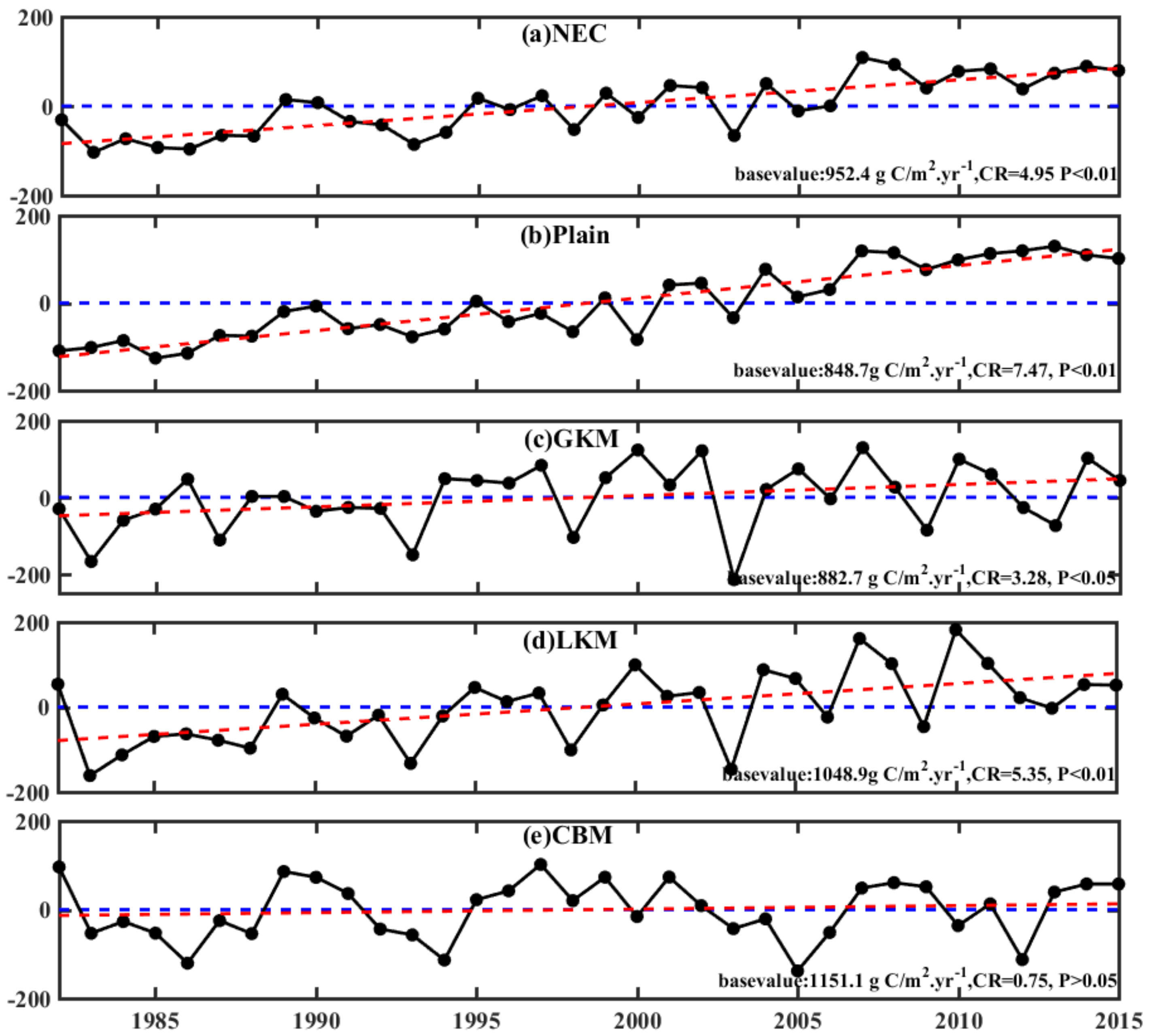
We further identified the inter-annual variation of zonal GPPGS at five regions: the whole NEC, plain, GKM, LKM, and CBM. There is an overall increasing trend of the whole NEC (the change ratio (denoted as CR, hereafter) = 4.95 g C/m2. yr−2; p < 0.01) from 1982 to 2015 as shown in Figure 3a, which is mostly attributed to the growth of crops in the plain (Figure 3b). Crops growing in the NEC have a stable increase with the largest amplitude (CR = 7.47 g C/m2. yr−2; p < 0.01), while, in the other three forested regions, GPPGS shows a much smaller increasing trend (LKM: CR = 5.35 g C/m2. yr−2, p < 0.01; GKM: CR = 3.28 g C/m2. yr−2, p < 0.05; CBM: CR = 0.75, p > 0.05) with quite a bit of inter-annual fluctuation over the past three decades.

3.2. Relationship between GPPGS and Meteorological Factors

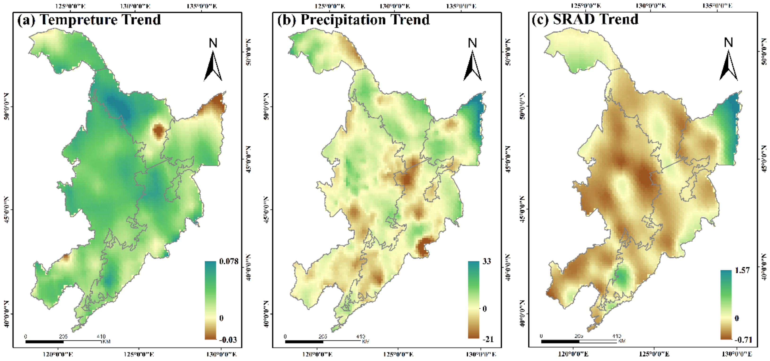
Figure 4 shows a warming, wetting, and dimming trend across the whole NEC, and the impacts of this climate change on vegetation GPPGS are analyzed in the following sections.
Table 1 indicates that GPPGS of the NEC is related with the three meteorological factors (daily average temperature, precipitation, and daily solar radiation), especially the obviously warming; nevertheless, this correlation has a great spatial heterogeneity. In plains, warming (Figure 4a) can improve the productivity of crops, while precipitation (Figure 4b) and solar radiation (Figure 4c) do not have significant impacts. In mountainous areas, positive impacts of warming on forest productivity only exist in high-latitude GKM and LKM, and solar radiation comes into positive effect on GPPGS in GKM and CBM. Precipitation has a negative effect on GPPGS of forests according to the correlation results, nevertheless, those negative effects were not significant when eliminating the coupling effects between temperature and radiation with precipitation as partial correlation coefficients display. The difference in correlation and partial correlation results manifest that in the NEC, precipitation indirectly impacts vegetation growth by affecting temperature and solar radiation. For example, there is a remarkable dip in GPPGS time series of the GKM and LKM in 2003 (Figure 3b,c), which is in line with the small amount of radiation caused by extreme large quantities of precipitation in 2003.
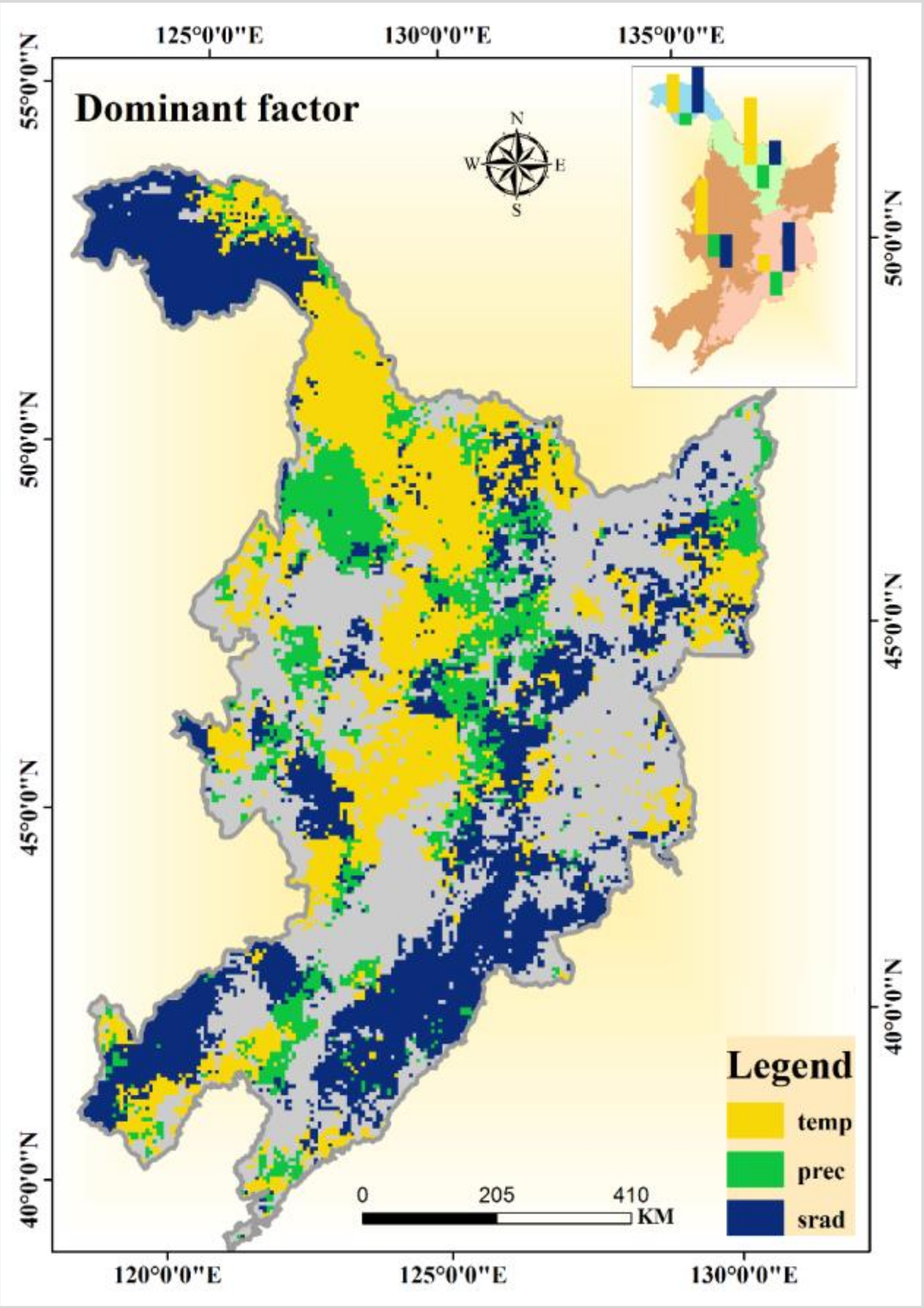
The contribution of each meteorological factors on GPPGS can be quantified using the SMLR method, and thus the dominant meteorological factors for GPPGS variation over the last three decades can be identified as shown in Figure 5. In mountainous areas, the combination of the three meteorological factors has great impacts on forest productivity. The inset map in Figure 5 shows that 70.5% of the GPPGS variation in LKM is caused by these three factors among which temperature is the dominant factor. Meteorological factors can explain 61.0% of the variation in GPPGS of CBM where solar radiation is the dominant factor. In GKM, climate effects accounts for 84.0% of the variation in GPPGS, and both temperature and solar radiation are equally important for vegetation productivity.
Contrary to productivity of natural forests in mountainous areas, crops growing in plain are less related with the three meteorological factors, although warming still has positive effect on vegetation productivity in some areas. Furthermore, the linear combination of temperature, precipitation, and solar radiation can only explain 40% of the significant GPPGS increase in crops, indicating that some other facilitating factors exist for crop productivity increments in the NEC.

3.3. Relationship between GPP and LAI

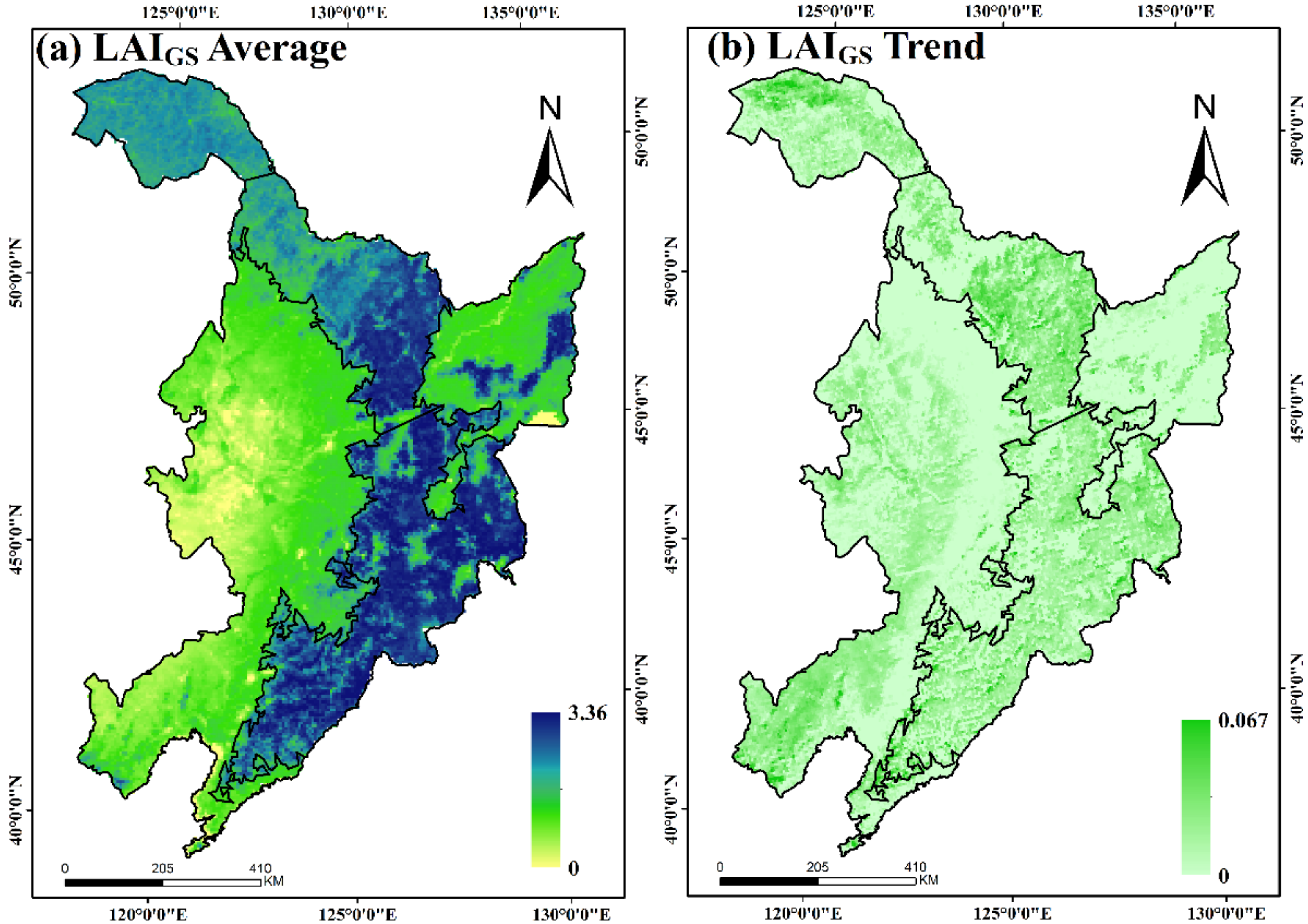
The comparison between GPP and LAI is noteworthy. We download GLASS-LAI products with an 8-day temporal resolution and 0.05° spatial resolution from 1982 to 2015 [39,53,54] and then pre-processed it to a 34-year time series of mean value of LAI within the growing season (denoted as LAIGS) across the whole NEC (Figure 6a). The detection of LAI trend across the NEC shows a dramatic increase in LAIGS across the whole NEC over the last 30 years (Figure 6b). It is the same as the widely reported worldwide greening [8,55,56,57].
Different from the significant increase in LAIGS across the whole NEC as Figure 6b shows, there is a relatively smaller increment of GPPGS in forested region across the NEC (the slight increment in the GKM and LKM, and even no increments of GPPGS in the CBM); quantitatively, the absolute change ratio (ACR) and relative change ratio (RCR, defined as A C R * s t u d y   p e r i o d m u l t i y e a r   m e a n   v a l u e ) of GPPGS and LAIGS in each part of the NEC are displayed in Table 2. In forested regions, the increments of LAIGS are larger than that of GPPGS, especially in CBM, while, in croplands, the RCR of GPPGS is twice that of LAIGS. The relationship between GPPGS and LAIGS seems to vary in different regions.
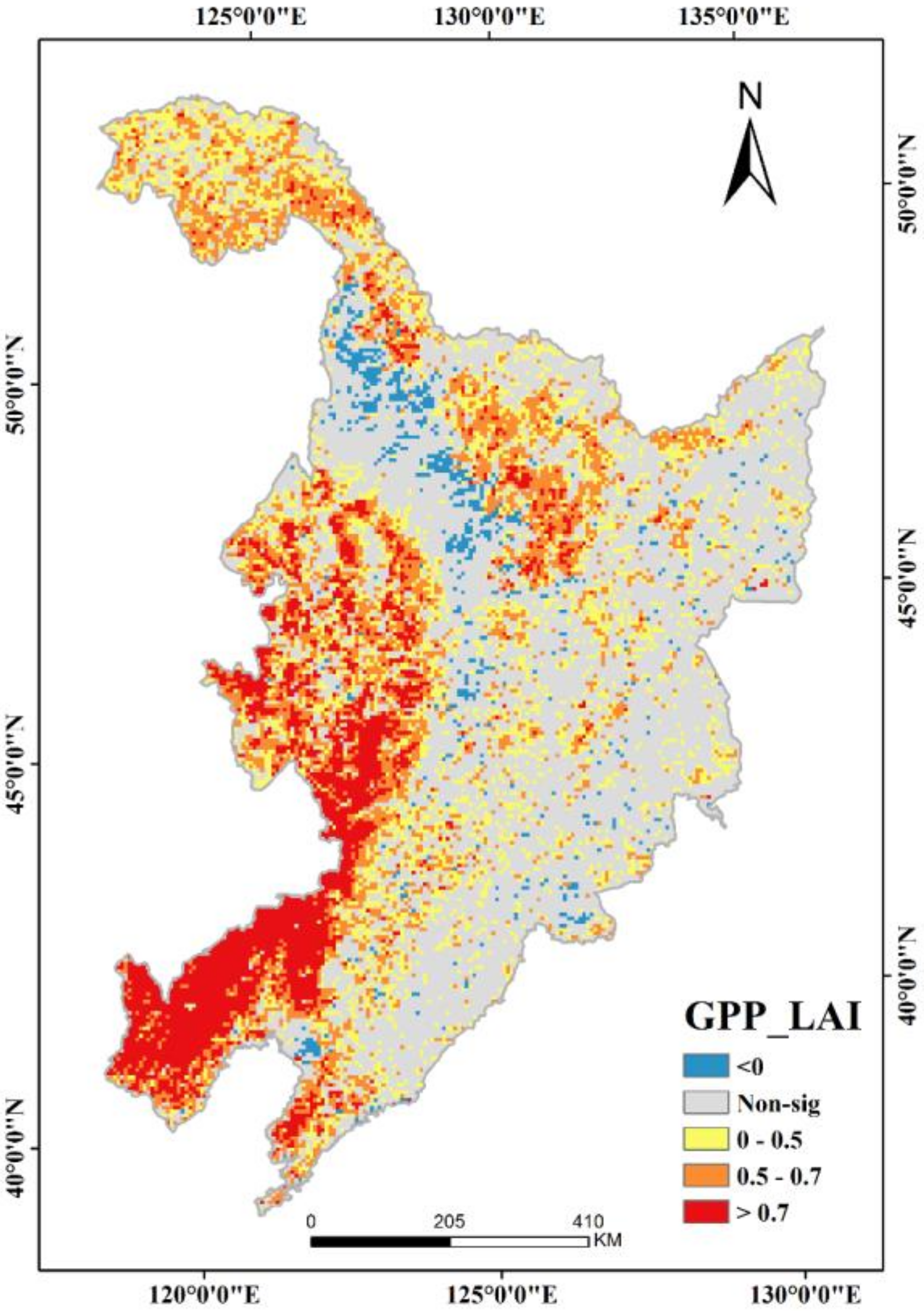
According to correlation analysis (Figure 7), GPPGS is correlated with LAIGS in relatively high-latitude forests (GKM: R = 0.652, p < 0.05; LKM: R = 0.691, p < 0.05) and parts of cropland; however, in mid-latitude CBM, there is non-significant correlation (R = 0.334; p > 0.05), indicating that GPP is not always changing simultaneously with LAI.

4. Discussion

4.1. Differences of Crops and Forests in GPPGS Trend

In both pixel or regional scales, the inter-annual variation trend of GPPGS in the NEC (Figure 2 and Figure 3) indicates that the crops growing in plains provide the majority inter-annual increments of terrestrial ecosystem productivity while forests in mountainous area contribute less in productivity increasing over the last 30 years. Furthermore, meteorological factors are not much important for crops in the NEC (Figure 5). Previous studies [58,59,60] identify two main reasons for the variation of crop productivity, i.e., climate change and agricultural technological progress. Fang et al. (2000) [60] concluded that agricultural technological progress plays a much more important role than climate for rice yield in Heilongjiang, which may be suited for the whole NEC.
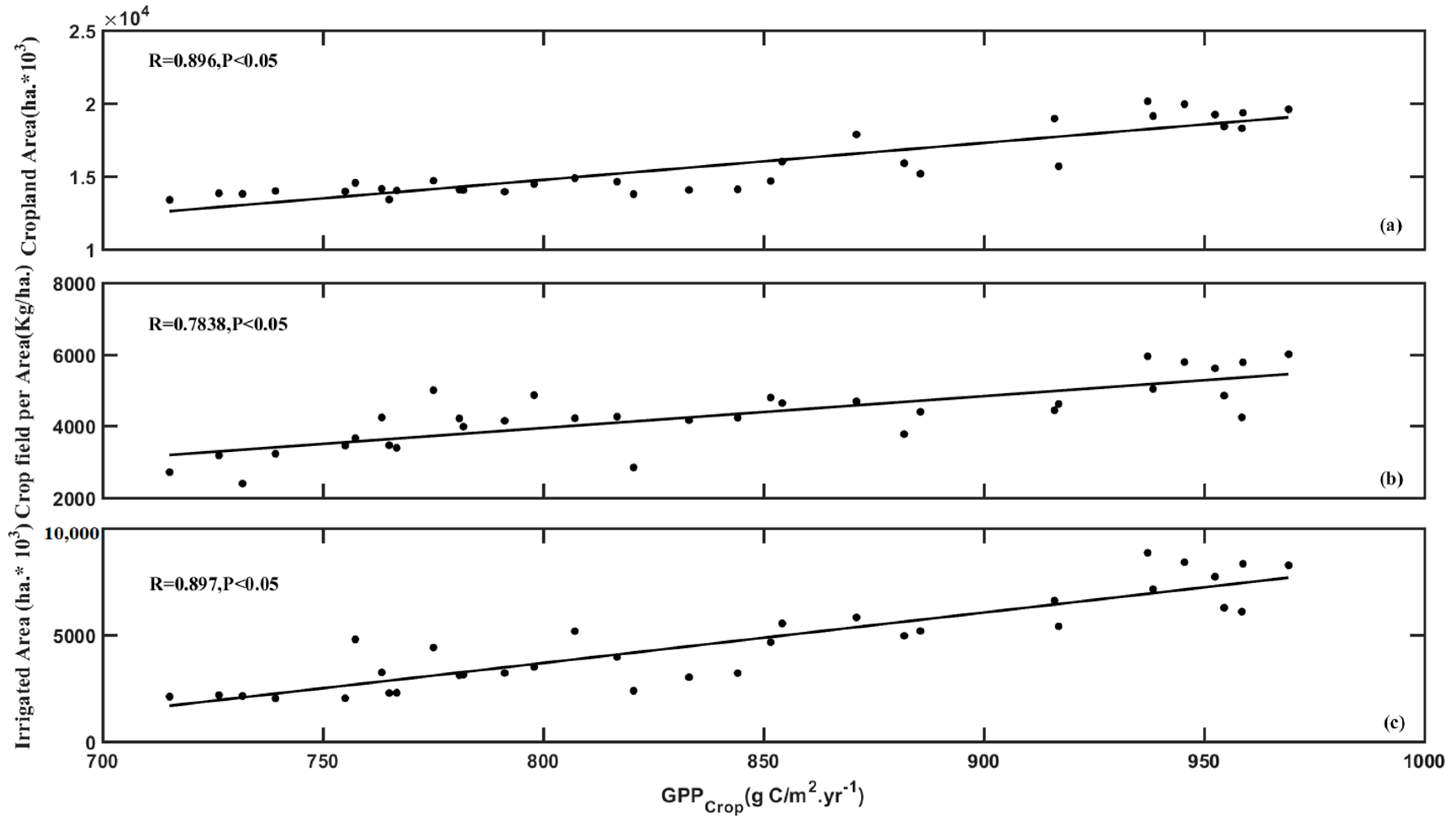
The relationship between GPPGS of crops and the three human intervention indices (IA, CA, and CYA) are displayed in Figure 8. All these indices are highly correlated with GPPGS where the IA (R = 0.897, p < 0.05) owns the largest correlation, followed by the CA (R = 0.896, p < 0.05), and finally, the CYA (R = 0.784, p < 0.05). The increments of vegetation productivity of crops in the NEC benefits greatly from human intervention (e.g., fertilization, irrigation, and cropland area expansion), instead of meteorological factors identified in Table 1, which is in line with Yuan’s findings [61].
All in all, human intervention contributes a lot to vegetation productivity of crops, which greatly facilitates vegetation growth of crops directly leading to the differences of crops and forests in GPP trend.

4.2. Different Trends of GPP and LAI

Song et al. (2017) [62] defined vegetation productivity as a combination of net assimilation rate, LAI, and photosynthesis duration. That is to say, apart from the LAI, net assimilation rate and photosynthesis duration are also decisive for GPP.
Firstly, the net assimilation rate is related with the vegetation type as well as vegetation age. There is a great spatial difference of vegetation type across the whole NEC as Figure 1b and Qian et al.’s study [63] display, so that the relationship between GPP and LAI has great spatial heterogeneity. In addition, the vegetation age is different with time went by which the correlation between GPP and LAI is also influenced. Second, combined with the correlation analysis between GPP and meteorological factors (Figure 5), we found that the CBM is a radiation-dominant region. so, the decreasing trend in solar radiation (or sunshine duration) (Figure 4c) may offset the effect of increasing LAIGS (Figure 6b), leading to non-significant variation in GPPGS over the 30 years.
Actually, LAI and GPP describes vegetation growth from two different aspects. LAI is defined as one half of the total green leaf area per unit horizontal ground surface area [64], which aims to quantify the amount of leaf area in an ecosystem [65], so in the NEC, the increasing LAIGS reflects that the leaf quantity and vegetation coverage of the canopy in the NEC increases, while the small variation in GPPGS indicates that vegetation’s contribution to regional carbon balance has not changed during the three decades of interaction with its environment across the NEC.
In summary, although LAIGS indicates a greening trend, ecological productivity may not have corresponding variation. GPPGS may be a more suitable parameter to reflect variation in vegetation growth and vegetation’s impacts on carbon cycle [1,2,3,4,5,6,7].

4.3. Uncertainties and Future Works

This paper has revealed the slight increasing of GPPGS in the NEC from 1982 to 2015, and simultaneously identified the effects of climate change on GPPGS. Nevertheless, some uncertainties still exist for this analysis.
First, we used the GLASS-GPP products which can provide vegetation productivity from 1982; however, the spatial resolution of GLASS-GPP (around 5 km) is rather rough, and thus some variations of GPP may be overlooked, especially in heterogeneous regions, leading to overestimation or underestimation of the trend of vegetation productivity.
Another uncertainty comes from correlation analysis between GPPGS and three meteorological factors. In this study, we chose the fixed growing season (April to October) of each year as our study period, and then considers the impacts of the three meteorological factors (daily average temperature, precipitation, and daily radiation) within the growing season, nevertheless, these three factors may influence vegetation growth during the whole year. Take temperature as an example, winter temperature also influences spring phenological events of the next year [66]. Therefore, using fixed growing season period as well as considering annual average temperature during growing season to analyze the effects of warming on vegetation productivity may bring some uncertainties. In the next step, we should consider a variable growing season length, such as using temperature thresholds (e.g., 0 and 5 °C) as a sign for growing season, so that a more comprehensive impact of meteorological factors on GPP can be taken into account.
Finally, uncertainty may exist when quantified the effects of each meteorological factors on GPP using SMLR models. The SMLR model assumed that the combined effect of meteorological factors is linear, actually, there is a more complex relationship between GPPGS and meteorology, in addition, there is a coupling effect between vegetation and atmospheric dynamics, that is to say, apart from the effect brought by climate change on vegetation, the variation of vegetation would impact climate simultaneously as a lot of studies [67,68,69] have revealed. The relationship between weather and vegetation is too complex to quantify using a statistic-based model. So, a land process models based on biochemical mechanisms, such as CABLE [70], ORCHIDEE [71], and LPJ [72], is needed for more accurate analysis. Apart from reducing uncertainties mentioned above, one important thing that needs further exploration is the relationship between GPPGS and LAIGS. This paper found that the relationship between GPPGS and LAIGS across the NEC has large spatial heterogeneity, indicating that the widely reported greening is not bound to have great contribution to improve carbon sink capability. Whether this relationship between GPPGS and LAIGS found in this paper is specific to the NEC or a common phenomenon in the terrestrial ecosystem is still to be seen.

5. Conclusions

This study focuses on the regional feedback of vegetation in the Northeast China (NEC) to the obvious climate change using GLASS GPP products as indicators. Results shows that, from 1982 to 2015, GPPGS across the NEC has an overall increasing trend (4.95 g C/m2. yr−2, p < 0.01) within which great spatial heterogeneity exists. Vegetation productivity of crops distributing in western NEC is the smallest but has the largest increment (7.47 g C/m2. yr−2, p < 0.01). On the contrary, vegetation productivity of forests is obvious larger than that of crops but only has slight increments in northern NEC (GKM: CR = 3.28 g C/m2. yr−2, p < 0.05; LKM: CR = 5.35 g C/m2. yr−2, p < 0.01) and non-significant variation in southern NEC (CBM).
Correlation analysis between GPPGS and meteorological factors indicates that warming can improve vegetation productivity of crops as well as forests located in temperature-limited high latitude (GKM and LKM), while this positive effect vanishes in mid-latitude CBM. In addition, for crops of the NEC, apart from the facilitating effect of warming, human intervention plays a decisive role in vegetation productivity increasing over the last 30 years, which directly leads to the difference of crops and forest in GPPGS trend.
Contrary to the slight or even non-significant variation of vegetation productivity in forested region, an obvious vegetation greening is found across the whole NEC. Correlation analysis between GPPGS and LAIGS over the last three decades illustrates that the simultaneously increment of GPPGS and LAIGS only exists in high-latitude NEC (GKM and LKM), while in other region, facilitating effect of greening on GPPGS may be offset by other factors, such as the shortage of solar radiation in CBM. The different variation trend of GPPGS and LAIGS reminds us that apart from focusing on vegetation growth dynamics (greening or browning), more attention should be paid on vegetation’s feedback to climate as well as its role in carbon cycle.

Author Contributions

Conceptualization, L.H. and W.F.; methodology, L.H.; formal analysis, L.H.; writing—original draft preparation, L.H.; writing—review and editing, W.F., W.Y., H.R., and Y.C.; funding acquisition, W.F. All authors have read and agreed to the published version of the manuscript.

Funding

This work was supported by the National Natural Science Foundation of China (grant No. 41971301) and the Major Research Development Program of China (2017YFE0122400, 2016YFD0300601).

Data Availability Statement

The data presented in this study are available on request from the corresponding author or from the reference website.

Acknowledgments

We thank “anonymous” reviewers for their original insights. We are also immensely grateful to the editor for their comments on the manuscript.

Conflicts of Interest

The authors declare no conflict of interest.

References

  1. Chapin, M.C.; Matson, P.A.; Mooney, H.A. Principles of Terrestrial Ecosystem Ecology, 2nd ed.; Springer: New York, NY, USA, 2002; p. 102. [Google Scholar]
  2. Beer, C.; Reichstein, M.; Tomelleri, E.; Ciais, P.; Jung, M.; Carvalhais, N.; Rödenbeck, C.; Arain, M.A.; Baldocchi, D.; Bonan, G.B.; et al. Terrestrial gross carbon dioxide uptake: Global distribution and covariation with climate. Science 2010, 329, 834–838. [Google Scholar] [CrossRef] [PubMed] [Green Version]
  3. Anav, A.; Friedlingstein, P.; Beer, C.; Ciais, P.; Harper, A.; Jones, C.; Murray-Tortarolo, G.; Papale, D.; Parazoo, N.C.; Peylin, P.; et al. Spatiotemporal patterns of terrestrial gross primary production: A review. Rev. Geophys. 2015, 53, 785–818. [Google Scholar] [CrossRef] [Green Version]
  4. Jensen, M.N. Consensus on ecological impacts remains elusive. Science 2003, 299, 38. [Google Scholar] [CrossRef]
  5. Cox, P.; Jones, C. Illuminating the modern dance of climate and CO2. Science 2008, 321, 1642–1644. [Google Scholar] [CrossRef]
  6. Battin, T.J.; Kaplan, L.A.; Findlay, S.; Hopkinson, C.S.; Marti, E.; Packman, A.I.; Newbold, J.D.; Sabater, F. The boundless carbon cycle. Nat. Geosci. 2009, 2, 598–600. [Google Scholar] [CrossRef]
  7. IPCC. Land Use, Land-Use Change, and Forestry. In Cambridge University Press; Cambridge University Press: Cambridge, UK, 2000; pp. 1–51. [Google Scholar]
  8. Zhu, Z.; Piao, S.L.; Myneni, R.B.; Huang, M.; Zeng, N. Greening of the earth and its drivers. Nat. Clim. Chang. 2016, 6, 791. [Google Scholar] [CrossRef]
  9. Chen, C.; Park, T.; Wang, X.; Piao, S.; Xu, B.; Chaturvedi, R.K.; Fuchs, R.; Brovkin, V.; Ciais, P.; Fensholt, R.; et al. China and India lead in greening of the world through land-use management. Nat. Sustain. 2019, 2, 122–129. [Google Scholar] [CrossRef] [PubMed]
  10. Monteith, J.L. Solar radiation and productivity in tropical ecosystems. J. Appl. Ecol. 1972, 9, 747–766. [Google Scholar] [CrossRef] [Green Version]
  11. Monteith, J.L. Climate and the efficiency of crop production in Britain. Phil. Trans. R. Soc. B 1977, 281, 277–294. [Google Scholar]
  12. Martínez, B.; Sanchez-Ruiz, S.; Gilabert, M.A.; Moreno, A.; Campos-Taberner, M.; García-Haro, F.J.; Trigo, I.F.; Aurela, M.; Brümmer, C.; Carrara, A.; et al. Retrieval of daily gross primary production over Europe and Africa from an ensemble of SEVIRI/MSG products. Int. J. Appl. Earth Obs. 2018, 65, 124–136. [Google Scholar] [CrossRef]
  13. Running, S.W.; Nemani, R.R.; Heinsch, F.A.; Zhao, M.; Reeves, M.; Hashimoto, H. A continuous satellite-derived measure of global terrestrial primary production. Bioscience 2004, 54, 547–560. [Google Scholar] [CrossRef]
  14. Chen, Y.; Gu, H.; Wang, M.; Gu, Q.; Ding, Z.; Ma, M.; Liu, R.; Tang, X. Contrasting Performance of the Remotely-Derived GPP Products over Different Climate Zones across China. Remote Sens. 2019, 11, 1855. [Google Scholar] [CrossRef] [Green Version]
  15. Ferreira, R.R.; Mutti, P.; Mendes, K.R.; Campos, S.; Marques, T.V.; POliveira, C.; Gonçalves, W.; Mota, J.; Difante, G.; Urbano, S.A.; et al. An assessment of the MOD17A2 gross primary production product in the Caatinga biome, Brazil. Int. J. Remote Sens. 2021, 42, 1275–1291. [Google Scholar] [CrossRef]
  16. Yuan, W.; Liu, S.; Zhou, G.; Zhou, G.; Tieszen, L.L.; Baldocchi, D.; Bernhofer, C.; Gholz, H.; Goldstein, A.H.; Goulden, M.L.; et al. Deriving a light use efficiency model from eddy covariance flux data for predicting daily gross primary production across biomes. Agric. For. Meteorol. 2007, 143, 189–207. [Google Scholar] [CrossRef] [Green Version]
  17. Yuan, W.; Liu, S.; Yu, G.; Bonnefond, J.M.; Chen, J.; Davis, K.; Desai, A.R.; Goldstein, A.H.; Gianelle, D.; Rossi, F.; et al. Global estimates of evapotranspiration and gross primary production based on MODIS and global meteorology data. Remote Sens. Environ. 2010, 114, 1416–1431. [Google Scholar] [CrossRef] [Green Version]
  18. Chen, Z. Spatiotemporal variation of productivity and carbon use efficiency of Northeast forests in China from 2000 to 2015. Chin. J. Appl. Ecol. 2019, 30, 1625–1632. [Google Scholar]
  19. Zhao, J.F.; Yan, X.D.; Jia, G.S. Simulation of carbon stocks of forest ecosystems in Northeast China from 1981 to 2002. Chin. J. Appl. Ecol. 2009, 20, 241–249. [Google Scholar]
  20. Zhao, X.L. Influence of climate change on agriculture in Northeast China in recent 50 years. J. Northeast Agric. Univ. 2010, 41, 144–149. [Google Scholar]
  21. Liu, Z.J.; Yang, X.G.; Wang, W.F.; Li, K.N.; Zhang, X.Y. Characteristics of agricultural climate resources in three provinces of Northeast China under global climate change. Chin. J. Appl. Ecol. 2009, 20, 2199–2206. [Google Scholar]
  22. Ye, D.Z. Simulation Research on Global Change in China; China Meteorology Press: Beijing, China, 1992. [Google Scholar]
  23. Guo, L.H.; Wu, S.H.; Zhao, D.S.; Yin, Y.H.; Leng, G.Y.; Zhang, Q.Y. NDVI-based vegetation change in Inner Mongolia from 1982 to 2006 and its relationship to climate at the biome scale. Adv. Meteorol. 2014, 1–12. [Google Scholar] [CrossRef]
  24. Hou, W.; Gao, J.; Wu, S.; Dai, E. Interannual variations in growing-season NDVI and its correlation with climate variables in the southwestern karst region of China. Remote Sens. 2015, 7, 11105–11124. [Google Scholar] [CrossRef] [Green Version]
  25. Wu, C.; Venevsky, S.; Sitch, S.; Yang, Y.; Wang, M.; Wang, L.; Gao, Y. Present-day and future contribution of climate and fires to vegetation composition in the boreal forest of China. Ecosphere 2017, 8, e01917. [Google Scholar] [CrossRef] [Green Version]
  26. Zoran, M.A.; Zoran, L.F.V.; Dida, A.I. Forest vegetation dynamics and its response to climate changes. In Proceedings of the Conference on Remote Sensing for Agriculture, Ecosystems, and Hydrology XVIII, Edinburgh, UK, 26–29 September 2016. [Google Scholar]
  27. Yuan, W.P.; Zheng, Y.; Piao, S.L.; Ciais, P.; Lombardozzi, D.; Wang, Y.P. Increased atmospheric vapor pressure deficit reduces global vegetation growth. Sci. Adv. 2019, 5. [Google Scholar] [CrossRef] [PubMed] [Green Version]
  28. Guo, J.T.; Hu, Y.M.; Xiong, Z.P.; Yan, X.L.; Li, C.L.; Bu, R.C. Variations in Growing-Season NDVI and Its Response to Permafrost Degradation in Northeast China. Sustainability 2017, 9, 551. [Google Scholar] [CrossRef] [Green Version]
  29. Hu, S.; Liu, J.; Mao, X.G. Extraction and Change of Vegetation Coverage of 2007–2010 in Northeast China. J. Northeast. For. Univ. 2017, 45, 45–50. [Google Scholar]
  30. Ni, X.L.; Xie, J.F.; Zhou, Y.K.; Gao, X.Z.; Ding, L. Evaluating vegetation growing season changes in northeastern China by using GIMMS LAI3g data. Climate 2017, 5, 37. [Google Scholar] [CrossRef] [Green Version]
  31. Zu, J.X.; Yang, J. Temporal variation of vegetation phenology in northeastern china. Acta Ecol. Sin. 2016, 36, 2015–2023. [Google Scholar]
  32. Yao, J.; He, X.Y.; Li, X.Y.; Chen, W.; Tao, D.L. Monitoring responses of forest to climate variations by Modis NDVI: A case study of Hun river upstream, northeastern china. Eur. J. Forest Res. 2012, 131, 705–716. [Google Scholar] [CrossRef]
  33. Tang, H.; Li, Z.; Zhu, Z.; Chen, B.; Zhang, B.; Xin, X. Variability and climate change trend in vegetation phenology of recent decades in the greater khingan mountain area, northeastern china. Remote Sens. 2015, 7, 11914–11932. [Google Scholar] [CrossRef] [Green Version]
  34. Liu, D.; Yu, C.L. Estimation on climatic productivity of vegetation NPP in northeastern china based on Modis. Res. Soil Water Conserv. 2017, 24, 315–323. [Google Scholar]
  35. Liu, X.; Guo, Q.; Wang, C. Simulating net primary production and soil-surface CO2 flux of temperate forests in Northeastern China. Scand. J. Forest Res. 2011, 26, 30–39. [Google Scholar] [CrossRef]
  36. Zhao, J.F.; Yan, X.D.; Guo, J.P.; Jia, G.S. Evaluating spatial-temporal dynamics of net primary productivity of different forest types in northeastern china based on improved FORCCHN. PLoS ONE 2012, 7. [Google Scholar] [CrossRef]
  37. Ji, Y.; Zhou, G.; Luo, T.; Dan, Y.; Zhou, L.; Lv, X. Variation of net primary productivity and its drivers in China’s forests during 2000–2018. Forest Ecosyst. 2020, 7, 15. [Google Scholar] [CrossRef] [Green Version]
  38. EarthData Search. Available online: https://search.earthdata.nasa.gov/ (accessed on 17 February 2021).
  39. Global Land Surface Satellite (GLASS) Products Download and Service. Available online: http://glass-product.bnu.edu.cn/ (accessed on 17 February 2021).
  40. National Center for Atmospheric Research Staff (Ed.) The Climate Data Guide: NASA MERRA. 10 June 2019. Available online: https://climatedataguide.ucar.edu/climate-data/nasa-merra (accessed on 17 February 2021).
  41. Savitzky, A.; Golay, M. Smoothing and differentiation of data by simplified least squares procedures. Anal. Chem. 1964, 36, 1627–1638. [Google Scholar] [CrossRef]
  42. He, J.; Yang, K.; Tang, W.; Lu, H.; Qin, J.; Chen, Y.Y.; Li, X. The first high-resolution meteorological forcing dataset for land process studies over China. Sci. Data 2020, 7, 25. [Google Scholar] [CrossRef] [Green Version]
  43. National Tibetan Plateau Third Pole Environment Data Center. Available online: http://westdc.westgis.ac.cn/data/ (accessed on 17 February 2021).
  44. Rodell, M.; Houser, P.R.; Jambor, U.E.A.; Gottschalck, J.; Mitchell, K.; Meng, C.J.; Arsenault, K.; Cosgrove, B.; Radakovich, J.; Bosilovich, M.; et al. The global land data assimilation system. Bull. Am. Meteorol. Soc. 2004, 85, 381–394. [Google Scholar] [CrossRef] [Green Version]
  45. Huffman, G.J.; Bolvin, D.T.; Nelkin, E.J.; Wolff, D.B.; Adler, R.F.; Gu, G.; Hong, Y.; Bowman, K.P.; Stocker, E.F. The TRMM Multisatellite Precipitation Analysis (TMPA): Quasi-Global, Multiyear, Combined-Sensor Precipitation Estimates at Fine Scales. J. Hydrometeorol. 2007, 8, 38–55. [Google Scholar] [CrossRef]
  46. Pinker, R.T.; Laszlo, I. Modeling surface solar irradiance for satellite applications on a global scale. J. Appl. Meteorol. 1992, 31, 194–211. [Google Scholar] [CrossRef] [Green Version]
  47. National Bureau of Statistics. Available online: http://www.stats.gov.cn/tjsj/ (accessed on 17 February 2021).
  48. Mann, H.B. Nonparametric tests against trend. Econometrica 1945, 13, 245–259. [Google Scholar] [CrossRef]
  49. Kendall, M.G. Rank Correlation Methods; Charles Grifin Company: London, UK, 1975. [Google Scholar]
  50. Patra, J.P.; Mishra, A.; Singh, R.; Raghuwanshi, N.S. Detecting rainfall trends in twentieth century (1871–2006) over Orissa state, India. Clim. Chang. 2012, 111, 801–817. [Google Scholar] [CrossRef]
  51. Yue, S.; Pilon, P. A comparison of the power of the t test, Mann– Kendall and bootstrap tests for trend detection. Hydrol. Sci. J. 2004, 49, 21–37. [Google Scholar] [CrossRef]
  52. Ay, M.; Kisi, O. Investigation of trend analysis of monthly total precipitation by an innovative method. Theor. Appl. Climatol. 2015, 120, 617–629. [Google Scholar] [CrossRef]
  53. Xiao, Z.Q.; Liang, S.L.; Wang, J.D.; Chen, P.; Yin, X.J.; Zhang, L.Q.; Song, J.L. Use of General Regression Neural Networks for Generating the GLASS Leaf Area Index Product from Time-Series MODIS Surface Reflectance. IEEE Trans. Geosci. Remote Sens. 2014, 52, 209–223. [Google Scholar] [CrossRef]
  54. Xiao, Z.Q.; Liang, S.L.; Wang, J.D.; Xiang, Y.; Zhao, X.; Song, J.L. Long-time-series global land surface satellite leaf area index product derived from MODIS and AVHRR surface reflectance. IEEE Trans. Geosci. Remote Sens. 2016, 54, 5301–5318. [Google Scholar] [CrossRef]
  55. Piao, S.; Yin, G.; Tan, J.; Cheng, L.; Huang, M.; Li, Y.; Liu, R.; Mao, J.; Myneni, R.B.; Peng, S.; et al. Detection and attribution of vegetation greening trend in china over the last 30 years. Glob. Chang. Biol. 2015, 21, 1601–1609. [Google Scholar] [CrossRef]
  56. Myneni, R.B.; Keeling, C.; Tucker, C.; Asrar, G.; Nemani, R. Increased plant growth in the northern high latitudes from 1981 to 1991. Nature 1997, 386, 698–702. [Google Scholar] [CrossRef]
  57. Nemani, R.R. Climate-driven increases in global terrestrial net primary production from 1982 to 1999. Science 2003, 300, 1560–1563. [Google Scholar] [CrossRef] [PubMed] [Green Version]
  58. Yun, Y.R.; Fang, X.Q.; Wang, Y.; Tao, J.; Qiao, T.F. Main Grain Crops Structural Change and Its Climate Background in Heilongjiang Province during the Past Two Decades. J. Nat. Resour. 2005, 20, 697–705. [Google Scholar]
  59. Wang, Z.Y.; Song, K.S.; Li, X.Y.; Zhang, B.; Liu, D.W. Effects of Climate Change on Yield of Maize in Maize Zone of Songnen Plain in the Past 40 Years. J. Arid Land Resour. Environ. 2007, 21, 112–117. [Google Scholar]
  60. Fang, X.Q.; Sheng, J.F. Human adaptation to climate change: A case study of changes in paddy planting area in Heilongjiang Province. J. Nat. Resour. 2000, 15, 213–217. [Google Scholar]
  61. Yuan, W.; Liu, S.; Liu, W.; Zhao, S.; Dong, W.; Tao, F.; Chen, M.; Lin, H. Opportunistic market-driven regional shifts of cropping practices reduce food production capacity of China. Earths Future 2018, 6, 634–642. [Google Scholar] [CrossRef] [Green Version]
  62. Song, Y.C. Vegetation Ecology, 2nd ed.; Higher Education Press: Beijing, China, 2017. [Google Scholar]
  63. Qian, H.; Yuan, X.Y.; Chou, Y.L. Forest Vegetation of Northeast China. In Forest Vegetation of Northeast Asia; Kolbek, J., Srutek, M., Box, O.E., Eds.; Springer: Amsterdam, The Netherlands; Berlin/Heidelberg, Germany, 2003; Chapter 6; pp. 181–230. [Google Scholar]
  64. Chen, J.M.; Black, T.A. Defining leaf area index for non-flat leaves. Plant Cell Environ. 1992, 15, 421–429. [Google Scholar] [CrossRef]
  65. Fang, H.; Baret, F.; Plummer, S.; Schaepman-Strub, G. An overview of global leaf area index (LAI): Methods, products, validation, and applications. Rev. Geophys. 2019, 57, 739–799. [Google Scholar] [CrossRef]
  66. Wang, H.J.; Wu, C.Y.; Ciais, P.; Penuelas, J.; Dai, J.H.; Fu, Y.S.; Ge, Q. Overestimation of the effect of climatic warming on spring phenology due to misrepresentation of chilling. Nat. Commun. 2020, 11, 4945. [Google Scholar] [CrossRef]
  67. Chen, C.J.; Chen, C.C.; Lo, M.H.; Juang, J.Y.; Chang, C.M. Central Taiwan’s hydroclimate in response to land use/cover change. Env. Res. Lett. 2020, 15, 034015. [Google Scholar] [CrossRef]
  68. He, Y.Q.; Lee, E.; Mankin, J.S. Seasonal tropospheric cooling in Northeast China associated with cropland expansion. Environ. Res. Lett. 2020, 15, 034032. [Google Scholar] [CrossRef]
  69. Pielke, R.A.; Mahmood, R.; McAlpine, C. Land’s complex role in climate change. Phys. Today 2016, 69, 40. [Google Scholar] [CrossRef] [Green Version]
  70. Wang, Y.P.; Law, R.M.; Pak, B. A global model of carbon, nitrogen and phosphorus cycles for the terrestrial biosphere. Biogeosciences 2010, 7, 2261–2282. [Google Scholar] [CrossRef] [Green Version]
  71. Krinner, G.; Viovy, N.; de Noblet-Ducoudré, N.; Ogée, J.; Polcher, J.; Friedlingstein, P.; Ciais, P.; Sitch, S.; Prentice, I.C. A dynamic global vegetation model for studies of the coupled atmosphere biosphere system. Glob. Biogeochem. Cycles 2005, 19, GB1015. [Google Scholar] [CrossRef]
  72. Sitch, S.; Smith, B.; Prentice, I.C.; Arneth, A.; Bondeau, A.; Cramer, W.; Kaplan, J.O.; Levis, S.; Lucht, W.; Sykes, M.T.; et al. Evaluation of ecosystem dynamics, plant geography and terrestrial carbon cycling in the LPJ dynamic global vegetation model. Glob. Chang. Biol. 2003, 9, 161–185. [Google Scholar] [CrossRef]
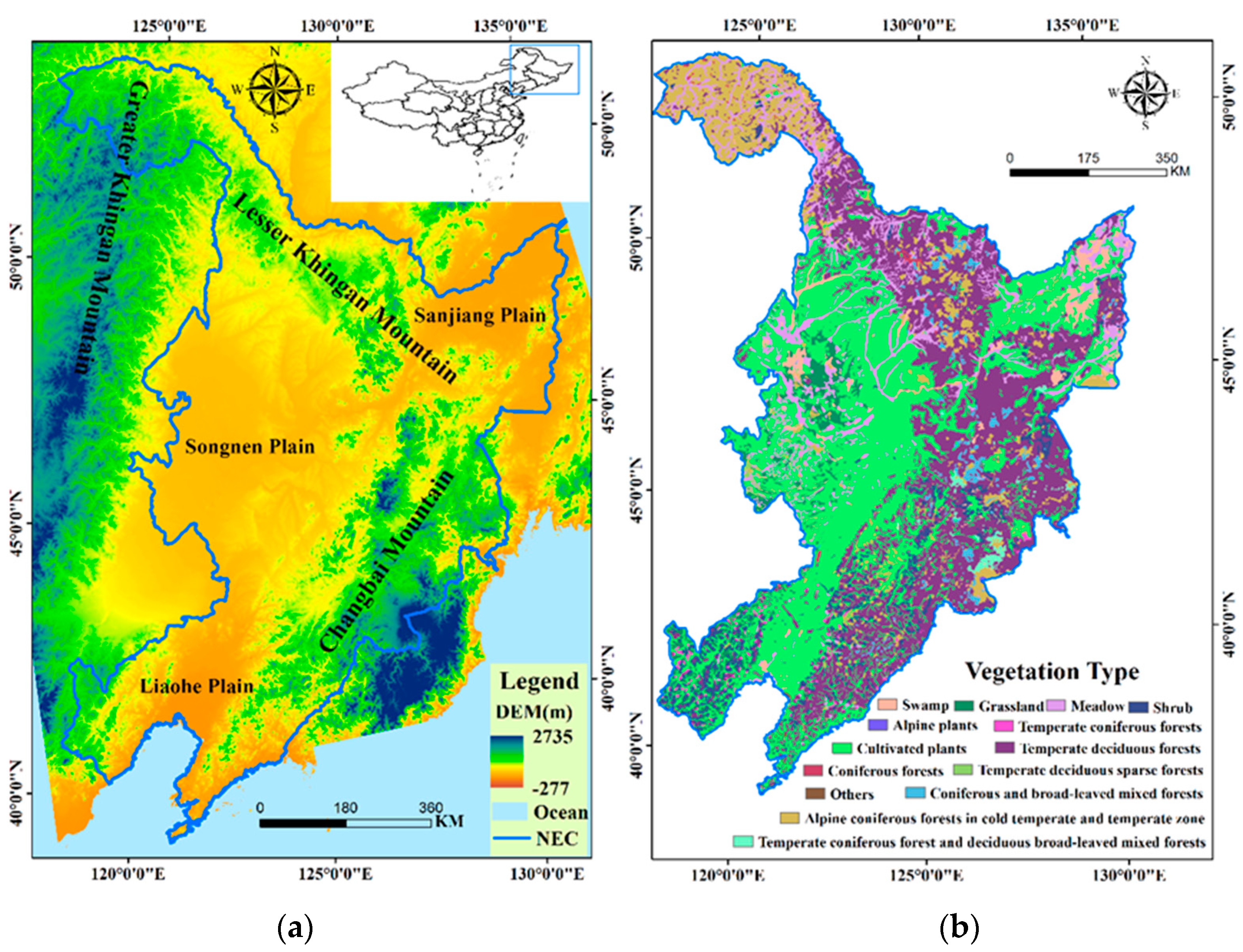
Figure 1. (a) Location of the study area with elevation from a Digital Elevation Model (DEM) and (b) Vegetation types of the Northeast China (NEC). (Vegetation type is provided by the Moderate Resolution Imaging Spectroradiometer (MODIS) MCD12Q1 datasets [38] in 2015).
Remotesensing 13 00951 g001
Figure 2. Spatial distribution of (a) multi-year average of accumulated gross primary productivity (GPPGS) (unit: g C/m2. yr−1) and (b) inter-annual GPPGS trend (unit: g C/m2. yr−2) across the NEC during 1982–2015.
Remotesensing 13 00951 g002
Figure 3. Trend of regional GPPGS anomalies (true value of GPPGS minus multi-average GPPGS) from 1982 to 2015 in five zones (the Greater Khingan Mountain (GKM), Lesser Khingan Mountain (LKM), the ChangBai Mountain (CBM), and Plain and the whole NEC) of the NEC (Here, the base value (the blue line) is the multi-year average GPPGS from 1982 to 2015; CR refers to the change ratio of GPPGS (g C/m2. yr−2), and P refers to the significance testing. The red line is a trend line calculated by the MK algorithm.).
Remotesensing 13 00951 g003
Figure 4. The inter-annual trend of (a) yearly average temperature, (b) yearly accumulated precipitation, and (c) yearly average SRAD (Shortwave Radiation) within the growing season across the NEC from 1982 to 2015.
Remotesensing 13 00951 g004
Figure 5. Dominant factors for GPPGS during 1982–2015 at pixel scale (main map) and at regional scale (the inset map).
Remotesensing 13 00951 g005
Figure 6. Spatial distribution of (a) multi-year average mean value of LAI within the growing season (LAIGS) and (b) trend in LAIGS across the NEC from 1982 to 2015.
Remotesensing 13 00951 g006
Figure 7. Spatial distribution of the correlation coefficient between GPPGS and LAIGS across the entire NEC.
Remotesensing 13 00951 g007
Figure 8. Relationship of GPPGS with (a) Cropland Area, (b) Crop Yield per Area, and (c) Irrigated Area.
Remotesensing 13 00951 g008
Table 1. Correlation coefficient (CC) and Partial correlation coefficient (PCC) between regional accumulated GPP (GPPGS) and meteorological factors (daily average temperature, precipitation and daily solar radiation) in different regions (Plain, GKM refers to the Greater Khingan Mountain, LKM refers to the Lesser Khingan Mountain, and the CBM refers to the ChangBai Mountain).
TemperaturePrecipitationSolar Radiation
CCPCCCCPCCCCPCC
Plain0.467 **0.479 **0.018−0.149−0.134−0.218
GKM0.501 **0.512 **−0.433 **−0.1650.776 **0.695 **
LKM0.590 **0.628 **−0.376 *−0.2020.389 *0.189
CBM0.2380.177−0.483 **−0.1990.567 **0.391 *
* Significant at the 5% level; ** significant at the 1% level.
Table 2. The absolute change ratio (ACR) and relative change ratio (RCR) of GPPGS and mean value of LAI within the growing season (LAIGS) from 1982 to 2015 across the NEC.
GPPGSLAIGS
ACRRCRACRRCR
GKM2.8811.240.01422.26
LKM4.7715.510.01217.46
CBM0.792.330.01215.84
Plain7.34529.750.005715.18
Publisher’s Note: MDPI stays neutral with regard to jurisdictional claims in published maps and institutional affiliations.