Abstract
Information about the growth, productivity, and distribution of vegetation, which are highly relied on and sensitive to natural and anthropogenic factors, is essential for agricultural production management and eco-environmental sustainability in the Amur River Basin (ARB). In this paper, the spatial–temporal trends of vegetation dynamics were analyzed at the pixel scale in the ARB for the period of 1982–2013 using remotely sensed data of long-term leaf area index (LAI), fractional vegetation cover (FVC), and terrestrial gross primary productivity (GPP). The spatial autocorrelation characteristics of the vegetation indexes were further explored with global and local Moran’s I techniques. The spatial–temporal relationships between vegetation and climatic factors, land use/cover types and hydrological variables in the ARB were determined using a geographical and temporal weighted regression (GTWR) model based on the observed meteorological data, remotely sensed vegetation information, while the simulated hydrological variables were determined with the soil and water assessment tool (SWAT) model. The results suggest that the variation in area-average annual FVC was significant with an increase rate of 0.0004/year, and LAI, FVC, and GPP all exhibited strong spatial heterogeneity trends in the ARB. For LAI and FVC, the most significant changes in local spatial autocorrelation were recognized over the Sanjiang Plain, and the low–low agglomeration in the Sanjiang Plain decreased continuously. The GTWR model results indicate that natural and anthropogenic factors jointly took effect and interacted with each other to affect the vegetated regime of the region. The decrease in the impact of precipitation to vegetation growth over the Songnen Plain was determined as having started around 1991, which was most likely attributed to dramatic changes in water use styles induced by local land use changes, and corresponded to the negative correlation between pasture areas and vegetation indexes during the same period. The analysis results presented in this paper can provide vital information to decision-makers for use in managing vegetation resources.
1. Introduction
As a major component of terrestrial ecosystems, vegetation plays an important role in material cycling and energy flows, and provides irreplaceable service functions that maintain the wellbeing of our planet and all the creatures that inhabit it. These function services include food provision, climate regulation, carbon sequestration, timber production, biodiversity preservation, and soil protection [1,2,3,4,5,6,7,8]. Vegetation growth affects the ecological balance, the terrestrial carbon cycle, water circulation, and other biochemical processes [2,9]. Thus, information about the spatial–temporal dynamics of regional and global vegetation is a fundamental need in order to facilitate the better management of our planet ecosystem, provide effective support for environmental sustainability and ensure the safety of agricultural production; these have become emerging issues in the field of environmental studies [2,5,10].
With the rapid advancement of remote sensing technology, global-scale land surface parameters, derived from long time series of remote sensing observations, have provided a good description of vegetation changes [11,12,13]. Leaf area index (LAI), defined as one-half the total developed area of green leaves per unit horizontal surface area, can serve as a proxy for detecting vegetation greenness and serves as a measure of the amount of vegetation that is vertically distributed [14,15,16,17,18,19]. Fractional vegetation cover (FVC), defined as the projected area of aboveground vegetation per unit ground area, can characterize the horizontal density of land surface vegetation and reflect plant community structure [20,21,22]. In addition, gross primary productivity (GPP) is the photosynthetic carbon assimilation by land plants per unit space and time, and can serve as an indicator of vegetation productivity [23,24,25]. Based on remote sensing products of these parameters at regional and global scales, scholars around the world have used different methods to study spatial–temporal changes in vegetation greenness (related to canopy structure) and vegetation productivity (related to canopy function) [26,27,28], such as trend analysis and spatial autocorrelation analysis.
Vegetation growth, production and distribution are highly reliant on—and sensitive to—natural and anthropogenic factors, such as precipitation, temperature, water resources, farming, and urban expansion. The condition of the global vegetation is constantly changing at various spatial and temporal scales, driven by natural and anthropogenic factors [29,30,31]. The response of vegetation dynamics to differences in environmental factors varies significantly across regions, according to the regional climate conditions, water availability, and land cover [32,33].
As the tenth largest river basin in the world, the natural conditions of the Amur River Basin (ARB), a transboundary basin in eastern Eurasia, vary greatly from region to region. In addition, the impact intensity of human activities on the ground vegetation has varied considerably under the influence of different national policies, lifestyles, and economic development [34,35,36,37,38]. In recent decades, significant climate changes have been observed in the ARB, where an annual mean temperature warming rate of about 0.34 °C/10a for 1975–2004 was reported, which is approximately 2.5 times higher than that for the 1891–2004 period [39]. Regional climatic characteristics and dramatic climate change govern the spatial–temporal changes of vegetation in the basin. In the context of changes in climatic and hydrological factors, the continued intensification of agricultural activities, driven by the large demand for food and economic development, affects the vegetation dynamics in the ARB and threatens the ecosystem [40,41,42].
Most previous studies have used correlation analyses and regression models to reveal the factors driving changes in vegetation dynamics in the whole basin or sub-basins of the ARB. For example, the Pearson correlation analysis, applied to investigate the relationship between growing season and seasonal Normalized Difference Vegetation Index (NDVI) and climatic variations in the ARB, was reported in [37] and it was concluded that growing season NDVI was mainly regulated by precipitation. A linear trend analysis of vegetation, temperature, and precipitation, and a comparison between the correlation of NDVI–temperature and NDVI–precipitation in northeastern China was carried out by Mao, et al. [43]. However, the analysis methods used in most of the previous studies focused solely on a temporal scale or spatial scale, and therefore, they do not provide a comprehensive analysis to deal with variability between vegetation dynamics and environmental factors at both spatial and temporal scales simultaneously [44,45,46]. Additionally, a few efforts have been made to investigate the relationships between hydrological factors and vegetation dynamics in the ARB, with close interactions between hydrological factors and vegetation growth having been found in many studies [47,48,49]. Therefore, exploring the spatial–temporal vegetation dynamics and their relationships with climatic, anthropogenic, and hydrological factors in the ARB is essential for better understanding the mechanisms driving vegetation changes, and can provide more detailed scientific support for environmental sustainability and agricultural production management. The objectives of this study are specified as follows:
- Analyze the spatial trends of three parameters (LAI, FVC and GPP) that can be considered as representative of the growth condition of surface vegetation in the study region using Mann–Kendall and Sen’s slope methods to understand the spatial variability of vegetation growth conditions.
- Explore the spatial autocorrelation characteristics of vegetation indexes in the ARB, based on the results derived from Moran’s I technique on remotely sensed vegetation information, for determining the rapid shift of eco-system changes over previous decades.
- Utilize partial least squares regression (PLSR) and geographical and temporal weighted regression (GTWR) models to further evaluate the relationships between land surface parameters and climatic factors, land use/cover types, and hydrological variables simulated with the soil and water assessment tool (SWAT) model in the ARB to clarify spatial–temporal vegetation dynamics and their relationships with climatic, anthropogenic, and hydrological factors in the Amur River Basin.
2. Study Area
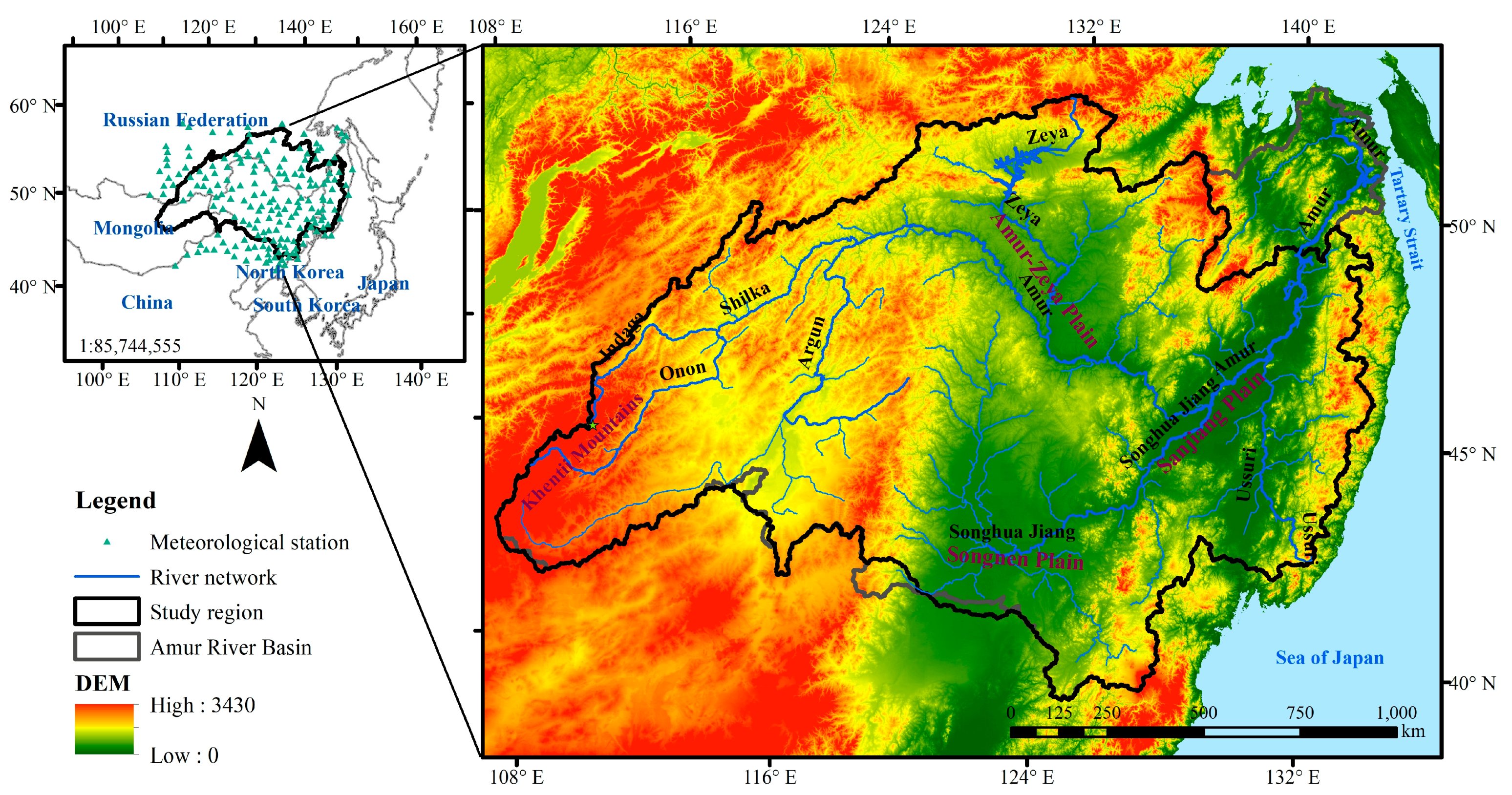
As the 10th largest river basin in the world, the ARB (41°–56° north and 107°–142° east) is situated in northeastern Asia. Its tributary rivers flow through China, Russia, Mongolia, and North Korea [36,38,41], covering a total land area of approximately 2 million square kilometers with elevations ranging from 0 (the mouth of the Amur River into the Tartary Strait) to 2565 m asl (the Khentii Mountains in northeastern Mongolia) [50,51] (See Figure 1). As one of the most important transnational river basins, the ARB exhibits quite different regional geographic and climatic characteristics: the topography is characterized by high mountains over the west, with typical continental climate features and low hills in east margin of the watershed, with an extensive plain in between, where the monsoonal climate is predominant. Population density presents a north–south gradient over the basin, with notable different anthropogenic effects [34,35,38]. Obtaining a better understanding of the vegetation dynamics driven jointly by natural and anthropogenic factors in the ARB, is therefore necessary for environmental sustainability studies. The hydrological variables derived from SWAT model simulations were confined in the sub-basin of the ARB where the Komsomolsk hydrological station gauged, covering 94% area of the whole ARB.
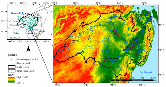
Figure 1.
Geographic map showing the location of the Amur River Basin in Eurasia with the topographic information attached and the locations of 193 meteorological stations used for this study.
3. Materials and Methods
3.1. Datasets
In this study, Global land surface satellite (GLASS) LAI, FVC and GPP products for the period of 1982–2013 were used to analyze vegetation dynamics. These GLASS products were released using the Hierarchical Data Format (HDF), accessible to the public for free at http://glass-product.bnu.edu.cn. The detailed information of land surface parameter products, representative of the vegetation dynamics used in this study are presented in Table 1. The monthly LAI and FVC values were computed using the maximum value composite (MVC) technique [52], which is widely used in compositing NDVI and other vegetation indexes in order to minimize the interference of atmospheric effects, the scan angle, cloud contamination, and solar zenith angle [29,53,54,55,56,57].

Table 1.
Land surface parameter products used in this study as representative of vegetation dynamics.
According to characteristics of climate changes during different periods in the ARB that have described in previous studies [61], in addition to the land use/cover transformations reported in the literature [36,40,62], the entire study period was divided into four periods to analyze the spatial–temporal relationships between environmental factors and vegetation dynamics: 1982–1990 (Period 1), 1991–1999 (Period 2), 2000–2006 (Period 3), and 2007–2013 (Period 4). The detailed information of datasets used in this study as representative of environmental factors are presented in Table 2. To investigate the driving factors of climate on vegetation changes, temperature and precipitation data observed from 1982 to 2013 in 193 meteorological stations within the basin were used. The climate data were interpolated at a spatial resolution of 8.8 × 8.8 km by using thin plate smoothing splines and Anusplin software, and the LAI, GPP, and FVC datasets in the same duration were resampled to the same spatial resolution. The combined datasets of Chinese land use maps with global land use maps from the closest dates in the four historical periods were used as inputs for the GTWR model to investigate the anthropogenic driving factors responsible for regional vegetation changes (urbanization and wetland reclamation, etc.). In addition, the hydrological variables simulated by the SWAT model, as presented in our previous study [61], were adopted to analyze the relationship between hydrological variables and vegetation dynamics.

Table 2.
Datasets used in this study as representative of environmental factors.
3.2. Methods
The paper presents the results of applying the Mann–Kendall, Sen’s Slope, and Global and Local Moran’s I techniques to analyze vegetation changes and applying PLSR and GTWR models to analyze the relationships between vegetation and climatic, anthropogenic, and hydrological factors based on meteorological data, remotely sensed information and hydrological variables simulated by the SWAT model. Figure 2 shows an overview of the general workflow followed in this study.
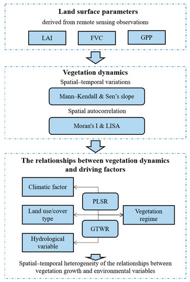
Figure 2.
Flowchart of investigating the spatial-temporal vegetation dynamics and their relationships with climatic, anthropogenic, and hydrological factors in the Amur River Basin (ARB). PLSR: partial least squares regression; GTWR: geographical and temporal weighted regression; LISA: local indicators of spatial association.
3.2.1. Time Trend Analysis
The magnitude of the trends in annual LAI, FVC and GPP were estimated using Sen’s slope method [63]. The median value of the slope series computed from two consecutive points of the series can help reduce the influence of outliers or missing data [63,64,65]. The formula of Sen’s slope method is as follows:
where and are the values at times i and j (), respectively, and a positive (negative) value of Slope indicates an upward (downward) trend.
The Mann–Kendall [66,67] non-parametric statistical test, which is frequently used to examine the significance of trends in time series of data, remining insensitive to outliers [23,68,69], was used to analyze the significance of the annual LAI, FVC, and GPP trends in each grid for the ARB during the 1982–2013 period. At a given significance level a = 0.05, the threshold of the normal distribution is (). When , the null hypothesis can be accepted (the trend is nonsignificant), and when , the trend is significant. The sequential version of the Mann–Kendall test proposed by Sneyers [68] was used to test abrupt changes in data series. If the intersection point of the forward sequence statistic UFk and the backward sequence UBk, which are calculated using the same equation but in reverse data series order, is between the boundary lines of the confidence zone ( at the confidence level of 95%), the critical point of change can be detected [70,71,72,73].
3.2.2. Spatial Autocorrelation Analysis
Spatial autocorrelation is the term used to describe the dependency and covariance of variables within a geographic area, and it reveals the phenomenon of geographic proximity’s potential [74,75]. In this paper, both global and local measures of spatial autocorrelation were calculated using the Python package GeoRasters to evaluate the degree of spatial autocorrelation in vegetation growth patterns across the study region and to indicate the variations in spatial autocorrelation throughout the study period [12,76].
Moran’s I [77] is one of the most commonly used indexes of global spatial autocorrelation. Moran’s I values range from −1 to 1: the index value from 0 to 1 indicates a positive autocorrelation, which implies a clustering state of spatial geographical phenomena, and the index value from −1 to 0 represents a negative autocorrelation, which implies a larger difference between neighbors, [74,78,79,80]. The formula for Moran’s I is given in Equation (2):
where and are the values of variable x (vegetation indexes) at location i and location j, respectively. is the average value of x, n is the total number of locations, and represents the spatial weight [4,44,81,82].
A local spatial autocorrelation analysis was performed using the local indicators of spatial association (LISA) [83,84] to indicate the spatial heterogeneity of the geographic phenomena at the local level across the study area, based on the following equation [74,83,85]:
where represents the variance of the observed values. In this study, the LISA map shows the spatial distribution (clustered/random/dispersed) of each vegetation index based on 9999 permutations at the significance level of p < 0.05. The spatial cluster/outlier characteristics of regions can be divided into four categories: low–low clusters (LL), high–high clusters (HH), low–high outliers (LH), and high–low outliers (HL). Positive and negative LISA values represent the aggregation of similar observations—“spatial cluster”, and different observations—“spatial outlier”, respectively [79,80,86,87,88,89].
3.2.3. GTWR
GTWR [45] was used in this study to reveal the spatial–temporal heterogeneity of the relationships between vegetation growth (LAI, FVC and GPP) and environmental variables (climatic, anthropogenic and hydrological factors) in the ARB at the sub-basin level [90]. Unlike the traditional geographically weighted regression model which considers only the spatial dimension, the GTWR model can well reflect evolution in the spatial–temporal relationships between vegetation dynamics and environmental variables and can simultaneously explore both spatial and temporal non-stationarity in vegetation changes [91,92]. The GTWR model can be expressed as follows:
where denotes the coordinates of location i in space and time; and are the dependent variable and the kth independent variable, respectively; represents the intercept value, is a set of parameter values at space–time location i; is the estimation of the parameters ; denotes the spatial–temporal weight matrix, and is the residual error.
4. Results
4.1. Spatial–Temporal Variations in Vegetation in the ARB
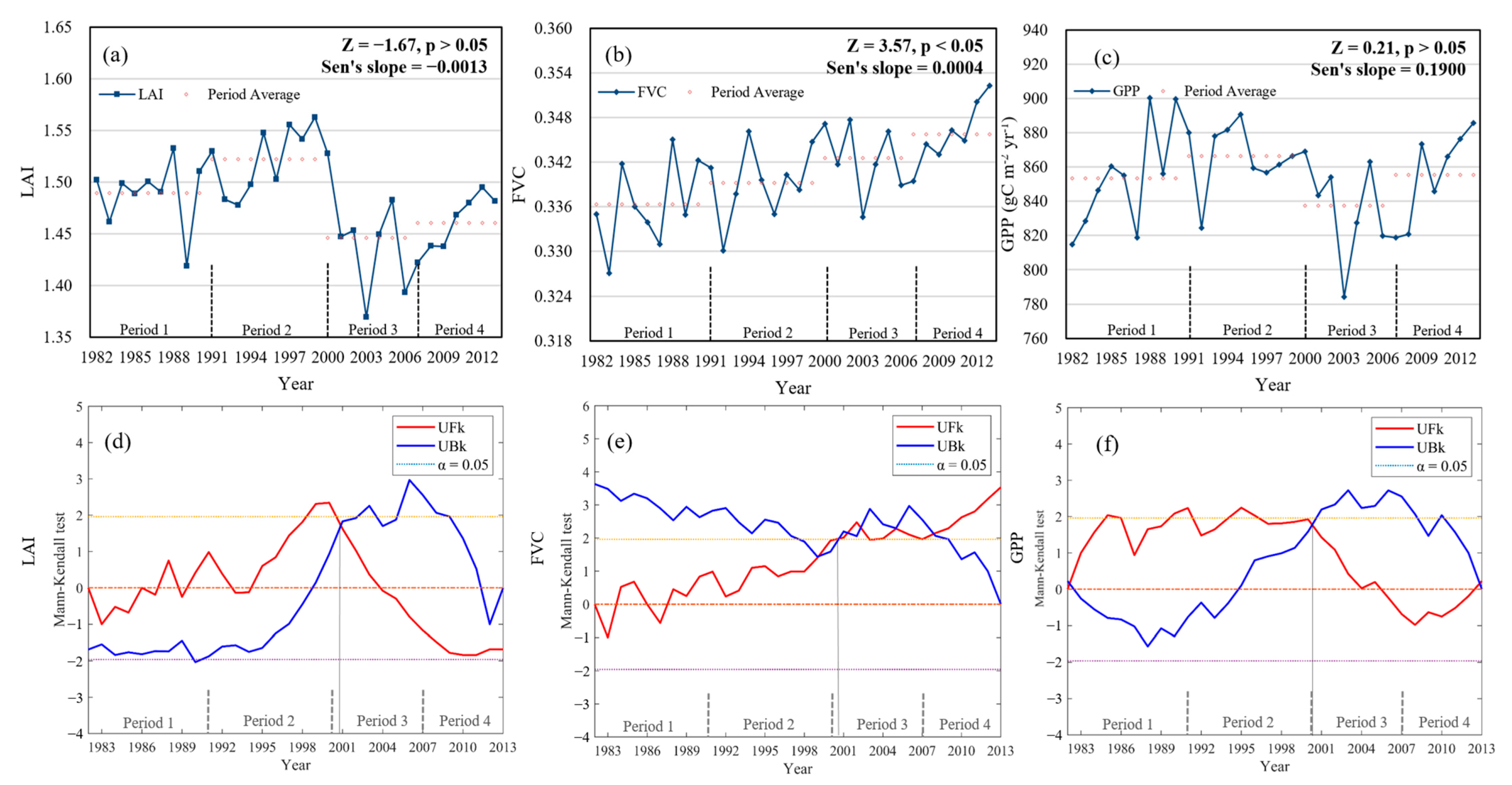
To detect the spatial–temporal variations of vegetation in the ARB basin, the Mann–Kendall test and Sen’s slope were employed to examine the trends and abrupt changes in the LAI, FVC and GPP from 1982 to 2013 at the confidence level of 95%. Figure 3a–c presents the Mann–Kendall Z value and Sen’s slope of the area-averaged annual vegetation indexes across the study region. During the study period, the annual FVC in the study region varied from a minimum of 0.327 in 1983 to a maximum of 0.352 in 2013 with a significant increase rate of about 0.0004/year (Z = 3.57, p < 0.05). While, the changes in area-averaged annual LAI in the same duration were not significant (Z = −1.67, p > 0.05), these values varied from a minimum of 1.369 in 2003 to a maximum of 1.563 in 1999, with a slight decreasing trend of −0.0013/year. Overall, an increasing trend at 0.19 gC m−2 yr−2 (Z = 0.21, p > 0.05) was found in annual GPP, however, large interannual fluctuations with a maximum value of 900.37 gC m−2 yr−1 (1988) and a minimum value of 784.05 gC m−2 yr−1 (2003) were observed. The period averages of LAI, FVC, and GPP for the four periods in Figure 3a–c indicated that the period averages of FVC gradually increased during the four periods, while the period averages of LAI and GPP changed most dramatically between Period 2 and Period 3 (before and after 2000).
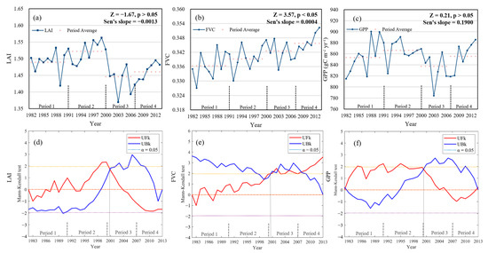
Figure 3.
Temporal changes in area-averaged annual LAI (a), FVC (b) and GPP (c), and sequential Mann–Kendall tests for the annual LAI (d), FVC (e) and GPP (f) with the forward-trend UFk and backward-trend UBk in the ARB during 1982–2013. p < 0.05 indicates significance at the 95% confident level.
The sequential Mann–Kendall tests for the annual LAI with a forward-trend UFk and backward-trend UBk, as illustrated in Figure 3d–f, indicated an obvious abrupt change in LAI in 2001. In addition, a significant abrupt change in GPP occurred in the study area around 2001. Several abrupt changes in FVC occurred from 1999 to 2008, but most of them were insignificant. These results suggested that all three types of indexes describing different vegetation statuses had undergone a rapid change around the year 2001.
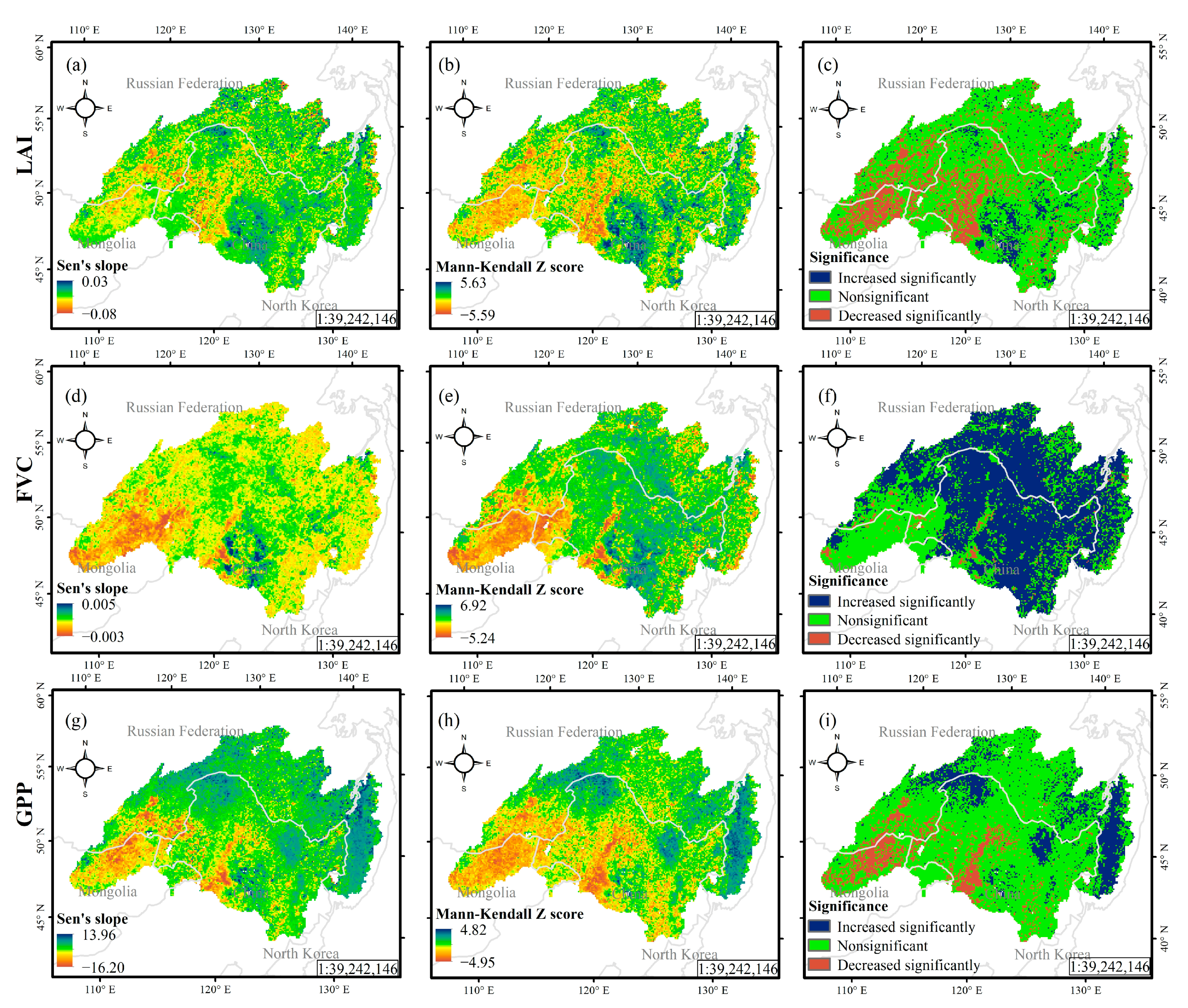
Figure 4a–i shows the spatial patterns of pixel-by-pixel Sen’s slope and the Mann–Kendall Z value estimated over the ARB, as well as the significance of the trends computed at a 95% significance level for the time series LAI, FVC and GPP images. Apparent spatial heterogeneity for the changes of LAI from 1982 to 2013 over the ARB, as exhibited in Figure 4a–c, was carefully investigated. The results indicated that about 37.3% of the basin area showed an increasing tendency in terms of LAI, in which approximately 7.7% tended to increase significantly (p < 0.05), where the most obvious increasing trend occurred over the Songnen Plain (an important food and oil production national base of China) in the southern part of the ARB. On the contrary, a decreasing trend in LAI was significant over about 18.9% of the ARB area, where the most significant reductions in LAI were mainly distributed in Mongolia and the Inner Mongolia Autonomous Region of China in the southwestern ARB area. Consistent with the area-averaged LAI trend, the LAI changes at the regional scale were insignificant over a large portion of the study area.
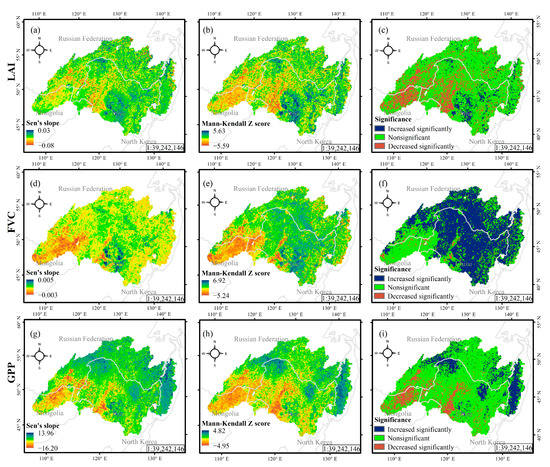
Figure 4.
Spatial patterns of Sen’s slope, the Mann–Kendall Z score and the significance of changes for the annual LAI (a–c), FVC (d–f) and GPP (g–i) from 1982 to 2013 in the ARB.
Over past 32 years in the ARB, 84.3% of the total basin area has exhibited an increasing trend in FVC, and pixels with a significant increasing trend accounted for about 62.5% of this value (p < 0.05), mainly being concentrated in the Chinese and Russian parts of the ARB. Only 2.0% of the total area showed a significantly decreasing trend, and pixels with a decreasing trend were mainly distributed in the southwestern margin of the ARB. For GPP, approximately 45.1% of the area in the ARB presented a decreasing trend, in which about 10.5% of the area was decreasing significantly (p < 0.05). Furthermore, areas with an increasing tendency accounted for 54.9% of the area, among which, 16.3% showed a significant increasing trend over the ARB from 1982 to 2013 (slope > 0, p < 0.05).
4.2. Spatial Autocorrelation Analysis of Vegetation Dynamics in the ARB
The global Moran’s I was investigated for the four period-averaged LAI, FVC, and GPP during 1982–2013 over the ARB. The global Moran’s I values of LAI for the four periods were 0.898, 0.897, 0.913 and 0.917 with p-values all being less than 0.01, respectively, which indicated a significant positive spatial autocorrelation and persistent high–high or low–low aggregations of the LAI. Similarly, the global Moran’s I values of FVC and GPP for the four stages were also all above 0.8, with p-values all less than 0.01, indicating positive spatial autocorrelation and persistent high–high or low–low aggregations. However, the global Moran’s I values do not indicate the possible spatial changes of spatial autocorrelation of the studied indexes across the basin.
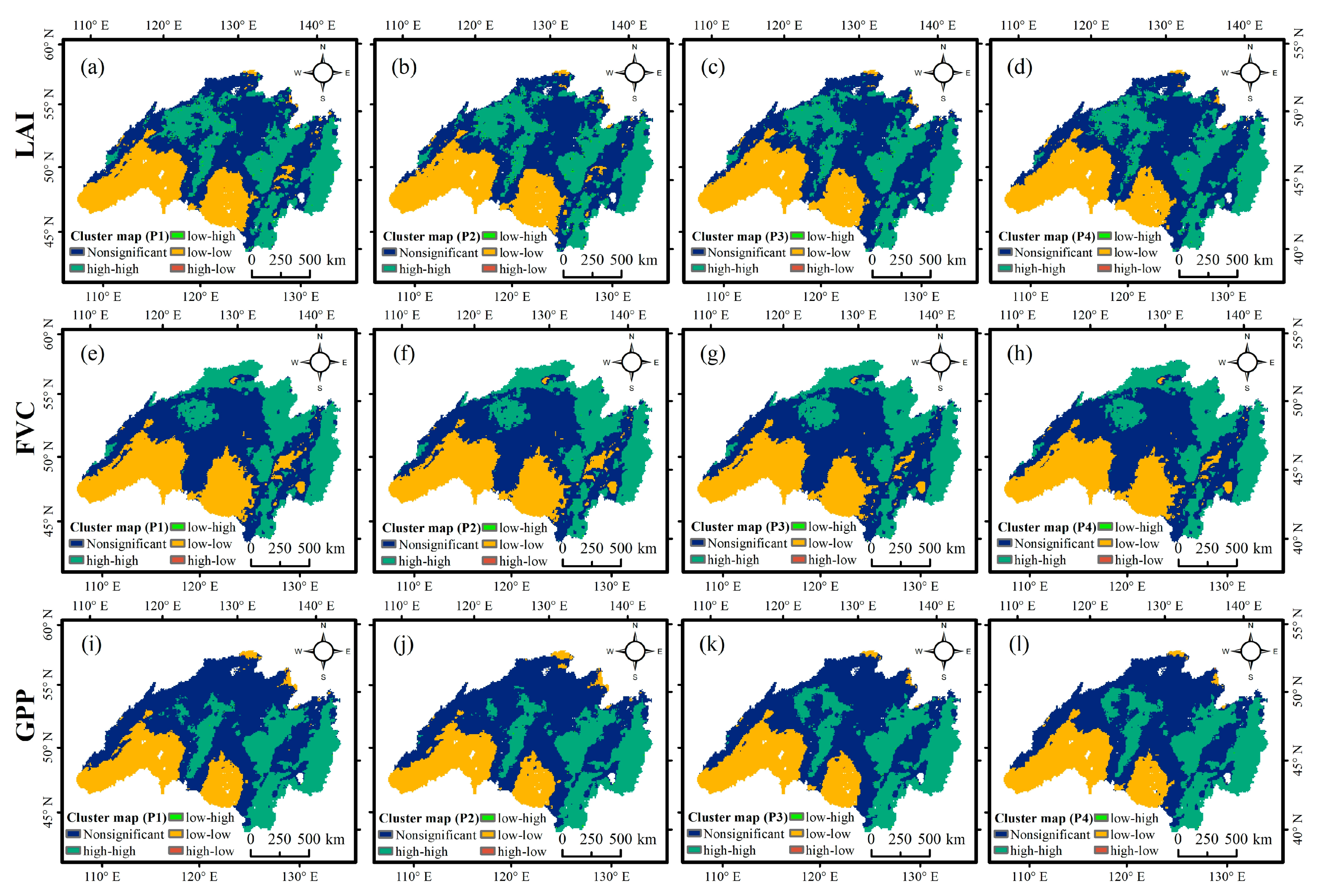
Figure 5 presents the clustering maps of the local Moran’s I of LAI, FVC and GPP in the ARB for the four studied periods (Figure 5a–d show Periods 1–4, respectively). The local Moran’s I for LAI in the four periods ranged from −1.83 to −10.41, −1.82 to 9.47, −1.57 to 5.55 and −0.90 to 5.93, respectively. With respect to the local Moran’s I of the LAI dataset for Periods 1–4, the areas of low–low agglomeration were always concentrated in the Mongolian region and the Songnen Plain and the Inner Mongolian Autonomous Region of China over four different phases. The clustering maps of the local Moran’s I values further revealed that the local spatial autocorrelation of the Sanjiang Plain demonstrated the most significant change and the low–low agglomeration in the Sanjiang Plain decreased persistently. Among these changes, the most significant changes were found between Period 2 and Period 3: i.e., the autocorrelation changed the most around 2000 over the Sanjiang Plain, while the low–low agglomeration in the Sanjiang Plain disappeared after 2000.
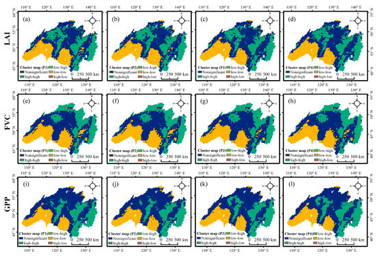
Figure 5.
Clustering maps of local Moran’s I of LAI, FVC and GPP in the ARB for four studied periods: (a–d) show clustering maps of LAI for Periods 1–4, respectively. (e–h) and (i–l) are the same as (a–d) of four studied periods, but for clustering maps of FVC and GPP, respectively.
Figure 5e–h presented the clustering maps of local Moran’s I of FVC in the ARB for four studied periods. The local Moran’s I of FVC for the four periods ranged from −0.67 to 6.45, −0.69 to 6.67, 0.57 to 6.21 and −0.65 to 6.63, respectively. Like the LAI spatial autocorrelation, the local spatial autocorrelations of FVC for the four periods were relatively stable, especially for the high–high agglomeration in the northern part of the basin. The clustering maps for the four periods all displayed strong high–high and low–low agglomerations, whereas the spatial outliers (high–low clustering or low–high clustering) were not conspicuous. A similar decreasing trend in low–low agglomeration areas in the Sanjiang Plain was also found during the study period.
Figure 5i–l presents the clustering maps of local Moran’s I of GPP in the ARB for four studied periods. The local Moran’s I of GPP for the four periods ranged from −1.77 to 8.24, −1.94 to 8.59, −1.70 to 6.27 and −1.90 to 6.93, respectively. For the four periods, the areas characterized with low–low agglomeration were always found in the Mongolia and the Songnen Plain and the Inner Mongolian Autonomous Region of China. Unlike that of the other two indexes, the spatial autocorrelation of GPP on the Sanjiang Plain changed very slightly, with no obvious low–low clustering in this area. The most significant changes in the clustering of GPP were found in Mohe County, the far most northern part of the Inner Mongolia Autonomous Region of China and the nearby border region with Russia; these areas exhibited a significant increase in high–high clustering.
4.3. The Relationships between Vegetation Dynamics and Changes in Climatic, Anthropogenic, and Hydrological Factors
As previously mentioned in Section 3.1, in order to analyze the relationship between vegetation status and climate changes, human activities and hydrological elements in the ARB, area-average climatic factors, land use area ratios, and simulated hydrological factors for 134 sub-basins—averaged annually over four phases—were used as explanatory variables to represent the environmental status of the ARB at different geographic locations and at different times. The statistical results of the explanatory variables in each sub-basin at different time periods are shown in Table 3.

Table 3.
Statistical results of period-average explanatory variables for four periods at the sub-basin scale.
However, analysis of the variance inflation factor (VIF) suggested a strong multi-collinearity between these independent variables (i.e., VIF > 10). In order to obtain more stable and accurate model results, a global analysis of relationships between vegetation indexes and environmental factors in the ARB were conducted using the PLSR model [93,94]; an appropriate model suitable for cases where multicollinearity between the independent or dependent variables exists. The independent variables were filtered using variable importance in the projection (VIP) values. The PLSR model results are summarized in Table 4, where strong (Adjusted R2 >0.8) relationships between vegetation indexes and environmental factors over the ARB can be observed.

Table 4.
Summary of the partial least squares regression (PLSR) modeled results over the ARB.
The VIP values of the independent variables are shown in Table 5. Independent variables with VIP values greater than one are usually considered as relatively important in a PLSR model. For further analysis, the independent variables with VIP values greater than 0.85 (Pcp, Tmax, Forest, Pasture, Surface runoff (SURQ), Amount of water stored in the soil profile (SW), and Snowmelt (SM)) were used as inputs for the GTWR model. Regionally averaged sub-basin LAI, FVC, and GPP values were used as dependent variable inputs.

Table 5.
Variable importance in the projection (VIP) values and beta coefficients of environmental factors in the PLSR model analysis.
The results of the GTWR models are summarized in Table 6. The results of the ordinary least squares regression (OLS) model, temporally weighted regression (TWR) model, and geographically weighted regression (GWR) model are also presented and were comparatively analyzed to verify the effectiveness of the GTWR model. The results indicated that the GTWR models of LAI, FVC, and GPP performed better than the other three models.

Table 6.
The summarized results of the ordinary least squares regression (OLS) model, temporally weighted regression (TWR) model, and geographically weighted regression (GWR) model for comparisons.
4.3.1. Regional Impacts of Climate Changes on Vegetation
As shown in Table 5, the global results of the PLSR model of the drivers prone to vegetation changes revealed the important role of Pcp in vegetation growth. Pcp is one of the factors among the independent variables that had a strong influence on LAI, FVC, and GPP (VIP > 1.5); in addition, the effects of Pcp on LAI, FVC, and GPP were all generally positive. Compared to Tmin and Tavg, Tmax and Pcp had a relatively strong effect on vegetation growth status, and the global results suggested that Tmax had a positive effect on LAI and GPP and a negative effect on FVC. Nevertheless, owning to significant spatial variability of climate changes over the study area [36,38], the relationships between vegetation and climate factors varied geographically, and thus, exhibited significant spatial heterogeneity.
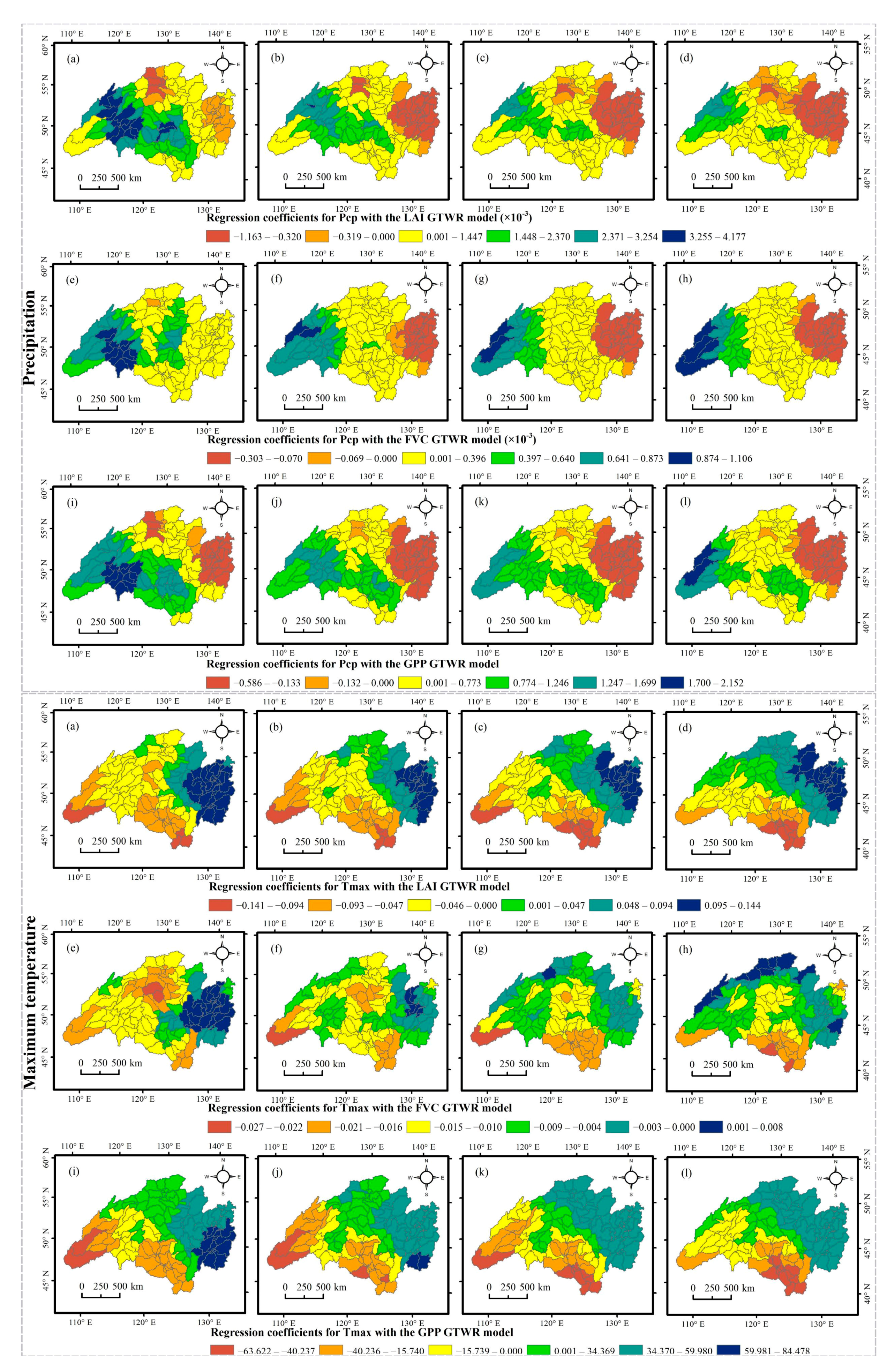
The spatial distributions of the regression coefficients for Pcp with the LAI, FVC and GPP GTWR models during the four studied periods are presented in the upper part of Figure 6. Although the effects of Pcp on LAI, FVC, and GPP differed in time and space, a general tendency for the coefficients is displayed on the figures: generally lower in the northeast and relatively higher in the southwest. The areas with high coefficient values were primarily concentrated at the borders of Mongolia, Russia, and China and near the Argun River Basin and the Shilka River Basin. Areas with relatively low coefficient values were found to be mostly distributed in the northeastern part of the basin, near the border of the Sanjiang Plain in China and in Khabarovsk Krai and the Jewish Autonomous Oblast in Russia. The area of negative Pcp regression coefficient values spread over time, or the intensity of the negative effect of Pcp increased.
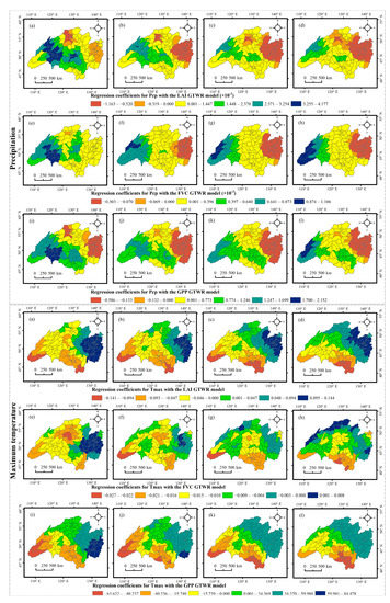
Figure 6.
The spatial distribution of the regression coefficients for Pcp and Tmax with the LAI ((a–d) present the coefficients for Periods 1–4, respectively), FVC ((e–h) show the coefficients for Periods 1–4, respectively), and GPP ((i–l) exhibit the coefficients for Periods 1–4, respectively) GTWR models for four studied periods.
The spatial distributions of the regression coefficients for Tmax with the LAI, FVC, and GPP GTWR models for the four studied periods are exhibited in the lower part of Figure 6. The effects of Tmax on LAI and GPP showed similar spatial and temporal patterns and, unlike the effects of Pcp, were roughly concentrated in high-value areas in the north and low-value areas in the south of the basin. The impact of Tmax on FVC, in contrast, had a distinct area of low values in the central part of the study area.
4.3.2. Regional Impacts of Land Use Changes on the Vegetation
In addition to climatic factors, anthropogenic activities that result in land use changes, such as farming, urbanization, and reforestation, also obviously affect the vegetation dynamics in the ARB. The PLSR model results (see Table 5) revealed that at the basin scale, the proportions of forest and pasture are the most important drivers for vegetation changes. Overall, the forest area posed a positive effect on all three indexes, while an increase in pasture area most likely resulted in the decreases in all three indexes.
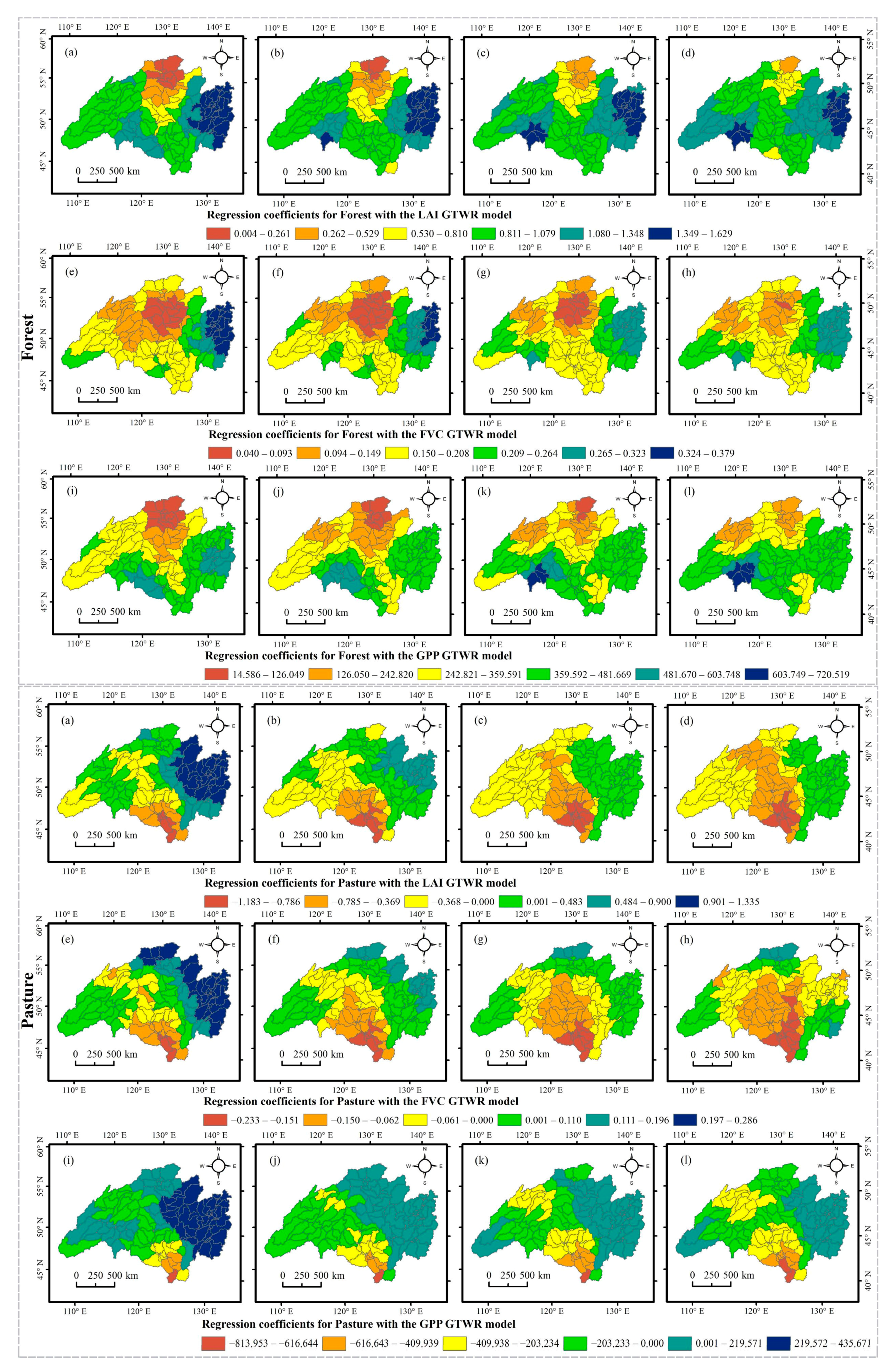
The upper part of Figure 7 presents the spatial distribution of the regression coefficients for forest with the LAI, FVC and GPP GTWR models for the studied four periods. From the perspective of the temporal and spatial distribution of the regression coefficients, the spatial distributions of the impacts of forest on LAI, FVC and GPP were very similar, and the spatial pattern varied slightly in the four studied periods. Regression coefficients for the forest over all sub-basins were greater than zero, and low values occurred in Huma County and Tahe County in China and Amur Oblast in Russia.
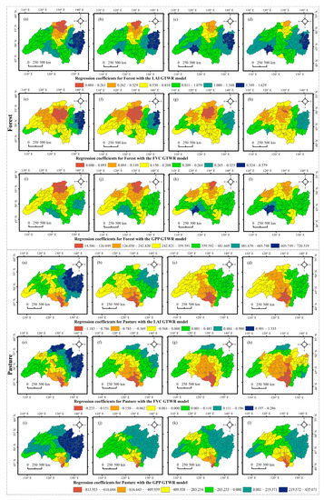
Figure 7.
The spatial distribution of the regression coefficients for forest and pasture with LAI ((a–d) display the coefficients for Periods 1–4, respectively), FVC ((e–h) show the coefficients for Periods 1–4, respectively), and GPP ((i–l) present the coefficients for Periods 1–4, respectively) GTWR models for the four studied periods.
According to the spatial distributions of the regression coefficients for pasture with the LAI, FVC and GPP GTWR models, as shown in the lower part of Figure 7, the negative values of the regression coefficients were mainly concentrated near the Songnen Plain in China. In addition, areas of high pasture influence on the three vegetation indexes have decreased in size and intensity over the four studied periods. Pasture had the strongest impact on vegetation in the northeastern ARB in Period 1, i.e., 1982–1990.
4.3.3. Spatial–Temporal Heterogeneity of the Relationships between Vegetation Dynamics and Hydrological Variables
Hydrological and ecological processes are interactive: on the one hand, the water cycle strongly influences the component structure, spatial distribution, and dynamics of plant communities; on the other hand, vegetation influences hydrological processes directly through root water uptake and stomatal transpiration; while indirectly through affecting water infiltration, slope runoff and evaporation processes via the vertical canopy structure and horizontal community distribution [95]. As shown in Table 5, the PLSR models predicted that SURQ, SW and SM were more closely related to vegetation growth than the other hydrological processes considered, and had similar levels of importance. Only SW was positively correlated with all three indexes, LAI, FVC, and GPP at the global scale.
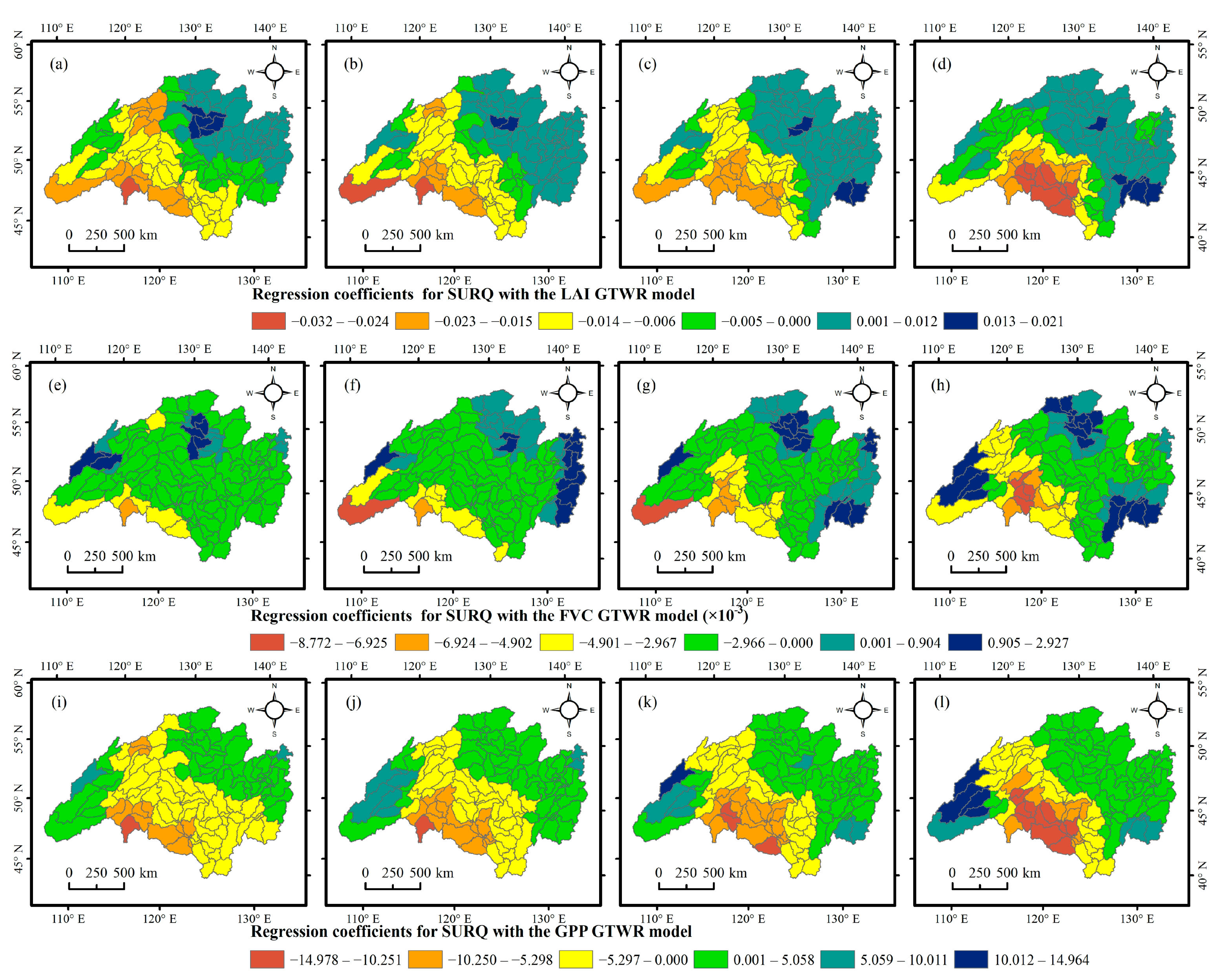
The spatial distribution of the regression coefficients for SURQ with the LAI, FVC and GPP GTWR models for the four studied periods are presented in Figure 8. Comparing the distributions of regression coefficients for SURQ with different vegetation indexes, it is clear that SURQ has the smallest range of positive regression coefficients in the FVC model. However, both the range and value of the positive coefficients in the FVC model showed an overall increasing trend during the study period.

Figure 8.
The spatial distribution of the regression coefficients for SURQ with the LAI ((a–d) shows the coefficients for Periods 1–4, respectively), FVC ((e–h) presents the coefficients for Periods 1–4, respectively), and GPP ((i–l) exhibits the coefficients for Periods 1–4, respectively) GTWR models for the four studied periods.
The spatial distribution of the regression coefficients for SW with the LAI, FVC and GPP GTWR models for the four studied periods are presented in Figure 9. In the region near the Argun River Basin in the western part of the study area, the relationship between SW and LAI, FVC and GPP generally showed a roughly positive to negative trend for the four studied periods. During Period 1 (1982–1990), the region with the highest positive values of the relationship between SW and LAI/GPP appeared in the middle of the watershed, near the China–Russia border, and differed from the distribution of regression coefficients in the FVC model. The values of the regression coefficients in this region decreased with time.
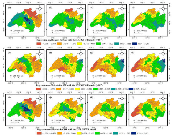
Figure 9.
The spatial distribution of the regression coefficients for SW with the LAI ((a–d) shows the coefficients for Periods 1–4, respectively), FVC ((e–h) illustrates the coefficients for Periods 1–4, respectively), and GPP ((i–l) presents the coefficients for Periods 1–4, respectively) GTWR models for the four studied periods.
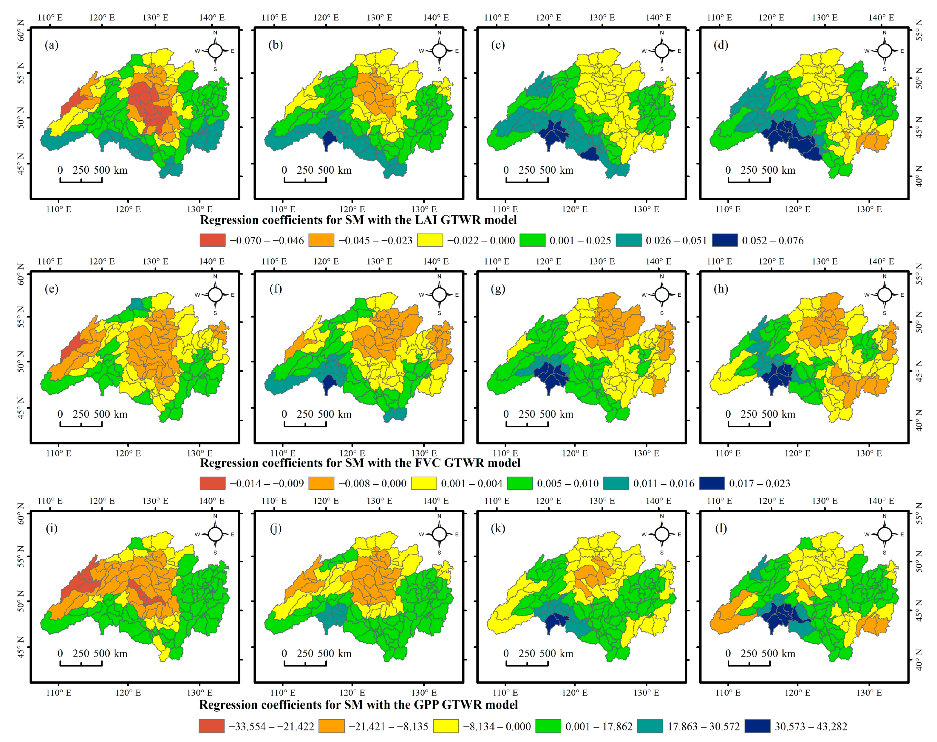
Figure 10 shows the spatial distribution of the regression coefficients for SM with the LAI, FVC and GPP GTWR models for the four studied periods. In comparison with Figure 8, Figure 9 and Figure 10, the results indicate that the relationship between the hydrological factors and LAI, FVC, or GPP differed significantly in terms of the spatial pattern. The spatial distribution of negative values of the regression coefficients for SURQ with the LAI and GPP models were more similar than that with the FVC model, and the regression coefficients for SW had the similar characteristics. In contrast, the regression coefficients for SM with the LAI, FVC and GPP models were more consistent in terms of spatial distribution, with a significant increase in the range of positive values in the study area between Period 1 and Period 2 (before and after 1991) and a decrease in the area of negative values in the middle of the study area.
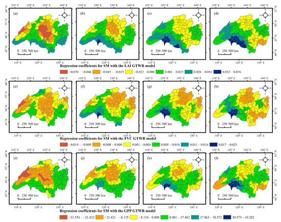
Figure 10.
The spatial distribution of the regression coefficients for SM with the LAI ((a–d) shows the coefficients for Periods 1–4, respectively), FVC ((e–h) exhibits the coefficients for Periods 1–4, respectively), and GPP ((i–l) presents the coefficients for Periods 1–4, respectively) GTWR models for the four studied periods.
5. Discussion
In this study, Mann–Kendall tests and Sen’s slope were employed to examine the trends and abrupt changes in the LAI, FVC and GPP from 1982 to 2013 in the ARB. The results suggest that the LAI, FVC, and GPP exhibited strong spatial heterogeneity trends with different spatial patterns. The area demonstrating significantly increased FVC values (p < 0.05), accounting for about 62.5% of the basin area, was larger than that presenting significantly increased LAI values (7.7%) and GPP values (16.3%). The areas of LAI, FVC and GPP that exhibited significant decreasing tends (p < 0.05) accounted for 18.9, 2.0 and 10.5% of the basin area, respectively. The differences in the vegetation dynamics indicated strong spatial variations in the impacts of environmental factors on vegetation growth conditions on the one hand, and different degrees of vegetation greenness and productivity—influenced by the environment—on the other hand. However, some similarities did exist in the spatial patterns of dynamic trends of LAI, FVC and GPP from 1982 to 2013 in the ARB. For example, all three indexes showed an overall increasing trend in the Songnen Plain and a decreasing trend in the Mongolian part of the ARB. However, a much more significant increasing trend was found in the LAI and FVC over the Songnen Plain, and much more significant decreasing trends in LAI and GPP were found over the Mongolian part of the ARB. In general, changes in the environmental factors of the Songnen Plain led to an increasing trend in the greenness and productivity of the vegetation in the region.
Despite the overall increasing trend of vegetation indexes in the Songnen Plain, local Moran’s I results showed that low–low aggregation of three indexes occurred in most areas of the region during the four studied phases. For LAI and FVC, the most significant changes in local spatial autocorrelation were recognized over the Sanjiang Plain, and the low–low agglomeration in the Sanjiang Plain decreased continuously. The different characteristics and stage changes in the spatial autocorrelation in the Sanjiang Plain and Songnen Plain, both of which are the food production bases of China, may be due to different planting structures.
The PLSR results suggested that Pcp, Tmax, Forest, Pasture, SURQ, SW, and SM were the major factors affecting LAI, FVC and GPP in the entire study region. The spatial distributions of regression coefficients for the GTWR models showed that the relationships between vegetation indexes and climate factors varied with geography, and thus, exhibited significant spatial heterogeneity. In general, areas with low Pcp coefficients were found to be mostly distributed in the northeastern part of the basin, near the border of the Sanjiang Plain in China and in Khabarovsk Krai and the Jewish Autonomous Oblast in Russia. The areas with relatively high coefficient values were primarily concentrated on the borders of Mongolia, Russia, and China and near the Argun River Basin and the Shilka River Basin. A temperate humid monsoon climate predominates the eastern part of the ARB, while the Mongolian region and the Argun River Basin—as well as the Shilka River Basin in the headwaters region of the western ARB—are less influenced by the Pacific coastal monsoon and characterize a continental arid–semi-arid climate [34]. Therefore, the area near the Argun River Basin and the Shilka River Basin showed a high degree of positive influence of Pcp during all four phases, which was most likely attributable to the relatively dry climate of this region.
In addition, comparisons among the spatial distributions of the regression coefficients for Pcp with the LAI, FVC and GPP GTWR models indicated that the area and intensity of the region of high Pcp coefficient values in northeastern China decreased from Period 1 to 2 (before and after 1991). Previous studies [96,97] have reported that large areas of pasture and wetland were converted into agricultural land—especially paddy fields—in this region during this period. With significant increases in rice cultivation in this region, the extensive river runoff interception and groundwater extraction were conducted to meet the demands of irrigation [96], which probably resulted in the weakened relationship between Pcp and regional vegetation growth. In addition, the continuous conversion of pasture to paddy field in the Songnen Plain may be one of the reasons for the negative impact of pastures on LAI, FVC and GPP in the region. These results suggested that natural and anthropogenic factors jointly took effect and interacted with each other, affecting the vegetation regime of the ARB.
The variations in the spatial patterns of the regression coefficients for the hydrological variables were generally more pronounced in time than those of the climatic factors, which is most likely attributable to more dramatic spatial–temporal changes in the hydrological processes. For example, the relationship between SW and GPP shifted from positive to negative in a large area of the southwestern part of the basin during Period 2 and Period 3 (before and after 2000). In addition, a significant increase in the range of positive SM coefficient values in the study area was found between Period 1 and Period 2 (before and after 1991). To some extent, the changes represent the increasingly apparent positive effect of SM runoff on vegetation growth in the study area during the period of 1982–1999. Comparing the distributions of regression coefficients for SURQ with different vegetation indexes, the smallest range of positive regression coefficients in the FVC model indicated that the relationship between surface runoff and vegetation productivity or vegetation vertical canopy distributions may be more positive than that with vegetation horizontal cover in the ARB. The impact of a single hydrological variable on the vegetation canopy structure and canopy function may vary in both direction (positive or negative) and intensity.
6. Conclusions
This study analyzed the spatial–temporal variations and spatial autocorrelation of vegetation growth conditions in the ARB at the pixel scale and investigated the spatial–temporal heterogeneity of the relationships between vegetation indexes and climatic, anthropogenic and hydrological factors at the sub-basin scale, using GTWR models from 1982 to 2013.
The trends of LAI, FVC and GPP in the ARB from 1982 to 2013 were quite different, but only the variation of area-average annual FVC proved to be significant with an increase rate of 0.0004/year (p < 0.05). All the annual vegetation indexes underwent a rapid change around the year 2001. Additionally, all three indexes showed an overall increasing trend in the Songnen Plain and a decreasing trend in the Mongolian part of the ARB during 1982–2013. The local Moran’s I results of LAI, FVC, and GPP suggested that similar decreasing trends in low–low agglomeration area of LAI and FVC on the Sanjiang Plain occurred during the study period.
According to the results of the GTWR models, the relationships between vegetation indexes and driving factors exhibited significant spatial–temporal heterogeneity. For example, a general tendency of the coefficients for Pcp existed: generally lower in the northeast and relatively higher in the southwest. The area near the Argun River Basin and the Shilka River Basin showed a high degree of positive influence on Pcp during all four phases, which was most likely attributed to the relatively dry climate in this region. Additionally, the negative values of regression coefficients for pasture were mainly concentrated near the Songnen Plain. The continuous conversion of pasture to paddy field may be one of the reasons for the negative impact of pastures on the vegetation dynamics in this region. SURQ had the smallest range of positive regression coefficients in the model for FVC among the three vegetation indexes, indicating that the relationship between surface runoff and vegetation productivity or vegetation vertical canopy distributions may be more positive than that with vegetation horizontal cover. Additionally, a significant increase in the range of positive regression coefficients for SM between Period 1 and Period 2 may suggest the increasingly apparent positive effect of SM runoff on vegetation growth in the study area during the period of 1982–1999.
Natural and anthropogenic factors jointly took effect and interacted with each other to affect the vegetated regime of the region. The decrease in the impact of precipitation on vegetation growth in the Songnen Plain was determined as having commenced around 1991, which was most likely attributable to dramatic changes in water use styles induced by local land use changes, and this corresponded to the negative correlation between pasture areas and vegetation indexes during the same period.
Author Contributions
Conceptualization, W.Z.; data curation, S.Z., S.W., B.Z. and Q.X.; formal analysis, S.Z.; methodology, W.Z.; software, S.Z.; Writing—original draft, S.Z.; writing—review and editing, W.Z. All authors have read and agreed to the published version of the manuscript.
Funding
This research was funded by the National Key R&D Program of China, grant numbers (2016YFA0602302) and (2018YFB0605603-04).
Institutional Review Board Statement
Not applicable.
Informed Consent Statement
Not applicable.
Data Availability Statement
The data presented in this study are openly available in FigShare at https://doi.org/10.6084/m9.figshare.13498542.v2, reference number [13498542].
Acknowledgments
Open discussions in weekly seminars with the graduate students in Wanchang Zhang’s group are acknowledged.
Conflicts of Interest
The authors declare no conflict of interest.
References
- Peng, W.F.; Kuang, T.T.; Tao, S. Quantifying influences of natural factors on vegetation NDVI changes based on geographical detector in Sichuan, western China. J. Clean Prod. 2019, 233, 353–367. [Google Scholar] [CrossRef]
- Liu, X.X.; Tian, Z.X.; Zhang, A.B.; Zhao, A.Z.; Liu, H.X. Impacts of Climate on Spatiotemporal Variations in Vegetation NDVI from 1982–2015 in Inner Mongolia, China. Sustainability 2019, 11, 768. [Google Scholar] [CrossRef]
- Zhang, Y.H.; Ye, A.Z. Spatial and temporal variations in vegetation coverage observed using AVHRR GIMMS and Terra MODIS data in the mainland of China. Int. J. Remote Sens. 2020, 41, 4238–4268. [Google Scholar] [CrossRef]
- Karasiak, N.; Dejoux, J.F.; Fauvel, M.; Willm, J.; Monteil, C.; Sheeren, D. Statistical Stability and Spatial Instability in Mapping Forest Tree Species by Comparing 9 Years of Satellite Image Time Series. Remote Sens. 2019, 11, 2512. [Google Scholar] [CrossRef]
- Akujärvi, A.; Lehtonen, A.; Liski, J. Ecosystem services of boreal forests—Carbon budget mapping at high resolution. J. Environ. Manag. 2016, 181, 498–514. [Google Scholar] [CrossRef] [PubMed]
- Li, B.; Chen, D.; Wu, S.; Zhou, S.; Wang, T.; Chen, H. Spatio-temporal assessment of urbanization impacts on ecosystem services: Case study of Nanjing City, China. Ecol. Indic. 2016, 71, 416–427. [Google Scholar] [CrossRef]
- Zhao, A.Z.; Zhang, A.B.; Lu, C.Y.; Wang, D.L.; Wang, H.F.; Liu, H.X. Spatiotemporal variation of vegetation coverage before and after implementation of Grain for Green Program in Loess Plateau, China. Ecol. Eng. 2017, 104, 13–22. [Google Scholar] [CrossRef]
- Du, Z.Q.; Zhao, J.; Pan, H.H.; Wu, Z.T.; Zhang, H. Responses of vegetation activity to the daytime and nighttime warming in Northwest China. Environ. Monit. Assess. 2019, 191, 10. [Google Scholar] [CrossRef] [PubMed]
- Gribovszki, Z.; Kalicz, P.; Balog, K.; Szabó, A.; Tóth, T.; Csáfordi, P.; Metwaly, M.; Szalai, S. Groundwater uptake of different surface cover and its consequences in great Hungarian plain. Ecol. Process. 2017, 6, 39. [Google Scholar] [CrossRef]
- Yang, Y.J.; Erskine, P.D.; Lechner, A.M.; Mulligan, D.; Zhang, S.L.; Wang, Z.Y. Detecting the dynamics of vegetation disturbance and recovery in surface mining area via Landsat imagery and LandTrendr algorithm. J. Clean Prod. 2018, 178, 353–362. [Google Scholar] [CrossRef]
- Wu, T.; Feng, F.; Lin, Q.; Bai, H.M. Advanced Method to Capture the Time-Lag Effects between Annual NDVI and Precipitation Variation Using RNN in the Arid and Semi-Arid Grasslands. Water 2019, 11, 1789. [Google Scholar] [CrossRef]
- Zhang, M.; Wang, J.M.; Li, S.J. Tempo-spatial changes and main anthropogenic influence factors of vegetation fractional coverage in a large-scale opencast coal mine area from 1992 to 2015. J. Clean. Prod. 2019, 232, 940–952. [Google Scholar] [CrossRef]
- Hua, L.; Wang, H.D.; Sui, H.G.; Wardlow, B.; Hayes, M.J.; Wang, J.X. Mapping the Spatial-Temporal Dynamics of Vegetation Response Lag to Drought in a Semi-Arid Region. Remote Sens. 2019, 11, 1873. [Google Scholar] [CrossRef]
- Chen, J.M.; Black, T.A. Measuring leaf-area index of plant canopies with branch architecture. Agric. For. Meteorol. 1991, 57, 1–12. [Google Scholar] [CrossRef]
- Chen, J.M.; Black, T.A. Defining leaf area index for non-flat leaves. Plant Cell Environ. 1992, 15, 421–429. [Google Scholar] [CrossRef]
- Li, X.J.; Qu, Y. Evaluation of Vegetation Responses to Climatic Factors and Global Vegetation Trends using GLASS LAI from 1982 to 2010. Can. J. Remote Sens. 2018, 44, 357–372. [Google Scholar] [CrossRef]
- Reygadas, Y.; Jensen, J.L.R.; Moisen, G.G.; Currit, N.; Chow, E.T. Assessing the relationship between vegetation greenness and surface temperature through Granger causality and Impulse-Response coefficients: A case study in Mexico. Int. J. Remote Sens. 2020, 41, 3761–3783. [Google Scholar] [CrossRef]
- Verger, A.; Camacho, F.; García-Haro, F.J.; Meliá, J. Prototyping of Land-SAF leaf area index algorithm with VEGETATION and MODIS data over Europe. Remote Sens. Environ. 2009, 113, 2285–2297. [Google Scholar] [CrossRef]
- Xiao, Z.; Liang, S.; Wang, J.; Xiang, Y.; Zhao, X.; Song, J. Long-Time-Series Global Land Surface Satellite Leaf Area Index Product Derived From MODIS and AVHRR Surface Reflectance. IEEE Trans. Geosci. Remote Sens. 2016, 54, 5301–5318. [Google Scholar] [CrossRef]
- Liu, D.Y.; Jia, K.; Wei, X.Q.; Xia, M.; Zhang, X.W.; Yao, Y.J.; Zhang, X.T.; Wang, B. Spatiotemporal Comparison and Validation of Three Global-Scale Fractional Vegetation Cover Products. Remote Sens. 2019, 11, 2524. [Google Scholar] [CrossRef]
- Mu, S.J.; Yang, H.F.; Li, J.L.; Chen, Y.Z.; Gang, C.C.; Zhou, W.; Ju, W.M. Spatio-temporal dynamics of vegetation coverage and its relationship with climate factors in Inner Mongolia, China. J. Geogr. Sci. 2013, 23, 231–246. [Google Scholar] [CrossRef]
- Yunhao, C.; Peijun, S.; Xiaobing, L.; Jin, C.; Jing, L. A combined approach for estimating vegetation cover in urban/suburban environments from remotely sensed data. Comput. Geosci. 2006, 32, 1299–1309. [Google Scholar] [CrossRef]
- Xu, H.J.; Zhao, C.Y.; Wang, X.P. Spatiotemporal differentiation of the terrestrial gross primary production response to climate constraints in a dryland mountain ecosystem of northwestern China. Agric. For. Meteorol. 2019, 276, 15. [Google Scholar] [CrossRef]
- Yao, Y.T.; Wang, X.H.; Li, Y.; Wang, T.; Shen, M.G.; Du, M.Y.; He, H.L.; Li, Y.N.; Luo, W.J.; Ma, M.G.; et al. Spatiotemporal pattern of gross primary productivity and its covariation with climate in China over the last thirty years. Glob. Chang. Biol. 2018, 24, 184–196. [Google Scholar] [CrossRef]
- Schaefer, K.; Schwalm, C.R.; Williams, C.; Arain, M.A.; Barr, A.; Chen, J.M.; Davis, K.J.; Dimitrov, D.; Hilton, T.W.; Hollinger, D.Y.; et al. A model-data comparison of gross primary productivity: Results from the North American Carbon Program site synthesis. J. Geophys. Res. Biogeosci. 2012, 117, 15. [Google Scholar] [CrossRef]
- Zhong, Q.Y.; Ma, J.; Zhao, B.; Wang, X.X.; Zong, J.M.; Xiao, X.M. Assessing spatial-temporal dynamics of urban expansion, vegetation greenness and photosynthesis in megacity Shanghai, China during 2000–2016. Remote Sens. Environ. 2019, 233, 12. [Google Scholar] [CrossRef]
- Zhang, X.; Liao, C.; Li, J.; Sun, Q. Fractional vegetation cover estimation in arid and semi-arid environments using HJ-1 satellite hyperspectral data. Int. J. Appl. Earth. Obs. Geoinf. 2013, 21, 506–512. [Google Scholar] [CrossRef]
- Tong, S.Q.; Zhang, J.Q.; Ha, S.; Lai, Q.; Ma, Q.Y. Dynamics of Fractional Vegetation Coverage and Its Relationship with Climate and Human Activities in Inner Mongolia, China. Remote Sens. 2016, 8, 776. [Google Scholar] [CrossRef]
- Zhao, A.Z.; Zhang, A.B.; Liu, J.H.; Feng, L.L.; Zhao, Y.L. Assessing the effects of drought and “Grain for Green” Program on vegetation dynamics in China’s Loess Plateau from 2000 to 2014. Catena 2019, 175, 446–455. [Google Scholar] [CrossRef]
- Zhou, Y.; Pei, F.S.; Xia, Y.; Wu, C.J.; Zhong, R.; Wang, K.; Wang, H.L.; Cao, Y. Assessing the Impacts of Extreme Climate Events on Vegetation Activity in the North South Transect of Eastern China (NSTEC). Water 2019, 11, 2291. [Google Scholar] [CrossRef]
- Meng, Y.Y.; Liu, X.N.; Wu, L.; Liu, M.L.; Zhang, B.Y.; Zhao, S. Spatio-temporal variation indicators for landscape structure dynamics monitoring using dense normalized difference vegetation index time series. Ecol. Indic. 2019, 107, 11. [Google Scholar] [CrossRef]
- Vicente-Serrano, S.M.; Azorin-Molina, C.; Pena-Gallardo, M.; Tomas-Burguera, M.; Dominguez-Castro, F.; Martin-Hernandez, N.; Begueria, S.; El Kenawy, A.; Noguera, I.; Garcia, M. A high-resolution spatial assessment of the impacts of drought variability on vegetation activity in Spain from 1981 to 2015. Nat. Hazards Earth Syst. 2019, 19, 1189–1213. [Google Scholar] [CrossRef]
- Sebastian, D.E.; Ganguly, S.; Krishnaswamy, J.; Duffy, K.; Nemani, R.; Ghosh, S. Multi-Scale Association between Vegetation Growth and Climate in India: A Wavelet Analysis Approach. Remote Sens. 2019, 11, 2703. [Google Scholar] [CrossRef]
- Simonov, E.A.; Dahmer, T.D. Amur-Heilong River Basin Reader; Ecosystems Hongkong: Hong Kong, China, 2008. [Google Scholar]
- Haruyama, S.; Shiraiwa, T. Environmental Change and the Social Response in the Amur River Basin; Springer: Berlin/Heidelberg, Germany, 2014; Volume 5. [Google Scholar]
- Dai, C.; Wang, S.; Li, Z.; Zhang, Y.; Gao, Y.; Li, C. Review on hydrological geography in Heilongjiang River Basin. Acta Geogr. Sin. 2015, 70, 1823–1834. [Google Scholar] [CrossRef]
- Chu, H.; Venevsky, S.; Wu, C.; Wang, M. NDVI-based vegetation dynamics and its response to climate changes at Amur-Heilongjiang River Basin from 1982 to 2015. Sci. Total Environ. 2019, 650, 2051–2062. [Google Scholar] [CrossRef]
- Yan, B.; Xia, Z.; Huang, F.; Guo, L.; Zhang, X. Climate Change Detection and Annual Extreme Temperature Analysis of the Amur River Basin. Adv. Meteorol. 2016, 2016, 1–14. [Google Scholar] [CrossRef]
- Novorotskii, P. Climate changes in the Amur River basin in the last 115 years. Russ. Meteorol. Hydrol. 2007, 32, 102–109. [Google Scholar] [CrossRef]
- Zou, Y.C.; Wang, L.Y.; Xue, Z.S.; E, M.J.; Jiang, M.; Lu, X.G.; Yang, S.D.; Shen, X.J.; Liu, Z.M.; Sun, G.Z.; et al. Impacts of Agricultural and Reclamation Practices on Wetlands in the Amur River Basin, Northeastern China. Wetlands 2018, 38, 383–389. [Google Scholar] [CrossRef]
- Cui, M. Status quo of Wetlands of Heilongjiang River Valley and the Protection (in Chinese). For. Inventory Plan. 2006, 1, 75–78. [Google Scholar] [CrossRef]
- Mao, D.H.; He, X.Y.; Wang, Z.M.; Tian, Y.L.; Xiang, H.X.; Yu, H.; Man, W.D.; Jia, M.M.; Ren, C.Y.; Zheng, H.F. Diverse policies leading to contrasting impacts on land cover and ecosystem services in Northeast China. J. Clean Prod. 2019, 240, 11. [Google Scholar] [CrossRef]
- Mao, D.H.; Wang, Z.M.; Luo, L.; Ren, C.Y. Integrating AVHRR and MODIS data to monitor NDVI changes and their relationships with climatic parameters in Northeast China. Int. J. Appl. Earth Obs. Geoinf. 2012, 18, 528–536. [Google Scholar] [CrossRef]
- Tu, M.Z.; Liu, Z.F.; He, C.Y.; Fang, Z.H.; Lu, W.L. The relationships between urban landscape patterns and fine particulate pollution in China: A multiscale investigation using a geographically weighted regression model. J. Clean Prod. 2019, 237, 16. [Google Scholar] [CrossRef]
- Huang, B.; Wu, B.; Barry, M. Geographically and temporally weighted regression for modeling spatio-temporal variation in house prices. Int. J. Geogr. Inf. Sci. 2010, 24, 383–401. [Google Scholar] [CrossRef]
- Li, J.; Heap, A.D. A Review of Spatial Interpolation Methods for Environmental Scientists; Geoscience Australia: Canberra, Australia, 2008. [Google Scholar]
- Le Maitre, D.C.; Scott, D.F.; Colvin, C. A review of information on interactions between vegetation and groundwater. Water SA 1999, 25, 137–152. [Google Scholar]
- Ludwig, J.A.; Wilcox, B.P.; Breshears, D.D.; Tongway, D.J.; Imeson, A.C. Vegetation patches and runoff-erosion as interacting ecohydrological processes in semiarid landscapes. Ecology 2005, 86, 288–297. [Google Scholar] [CrossRef]
- Yang, Z.F.; Li, C.H.; Huang, G.H.; Cai, Y.P. Analysis of relationships between NDVI and climatic/hydrological parameters in the Yellow River basin. Int. J. Environ. Pollut. 2010, 42, 166–183. [Google Scholar] [CrossRef]
- Zha, F.; Liu, C.; Shi, R. Elevation Cluster Dataset Covering the Amur River Basin. Global Chang. Data Repos. 2016, 1. [Google Scholar] [CrossRef]
- Yuefei, H.; Tiejian, L.; Enze, L.; Jiaye, L.; Rui, B.; Chuang, L.; Ruixiang, S. Boundary Data of the Amur River Basin. Glob. Chang. Data Repos. 2016, 1. [Google Scholar] [CrossRef]
- Holben, B.N. Characteristics of maximum-value composite images from temporal AVHRR data. Int. J. Remote Sens. 1986, 7, 1417–1434. [Google Scholar] [CrossRef]
- Knyazikhin, Y.; Glassy, J.; Privette, J.L.; Tian, Y.; Lotsch, A.; Zhang, Y.; Wang, Y.; Morisette, J.T.; Votava, P.; Myneni, R.B.; et al. MODIS Leaf Area Index (LAI) and Fraction of Photosynthetically Active Radiation Absorbed by Vegetation (FPAR) Product (MOD 15) Algorithm Theoretical Basis Document-1999. Available online: https://modis.gsfc.nasa.gov/data/atbd/atbd_mod15.pdf (accessed on 18 February 2020).
- Shabanov, N.V.; Huang, D.; Yang, W.Z.; Tan, B.; Knyazikhin, Y.; Myneni, R.B.; Ahl, D.E.; Gower, S.T.; Huete, A.R.; Aragao, L.; et al. Analysis and optimization of the MODIS leaf area index algorithm retrievals over broadleaf forests. IEEE Trans. Geosci. Remote Sens. 2005, 43, 1855–1865. [Google Scholar] [CrossRef]
- Jiang, L.; Kogan, F.N.; Guo, W.; Tarpley, J.D.; Mitchell, K.E.; Ek, M.B.; Tian, Y.; Zheng, W.; Zou, C.-Z.; Ramsay, B.H. Real-time weekly global green vegetation fraction derived from advanced very high resolution radiometer-based NOAA operational global vegetation index (GVI) system. J. Geophys. Res. Atmos. 2010, 115, D11114. [Google Scholar] [CrossRef]
- Hashimoto, H.; Wang, W.L.; Milesi, C.; White, M.A.; Ganguly, S.; Gamo, M.; Hirata, R.; Myneni, R.B.; Nemani, R.R. Exploring Simple Algorithms for Estimating Gross Primary Production in Forested Areas from Satellite Data. Remote Sens. 2012, 4, 303–326. [Google Scholar] [CrossRef]
- Zhang, S.Q.; Chen, H.; Fu, Y.; Niu, H.H.; Yang, Y.; Zhang, B.X. Fractional Vegetation Cover Estimation of Different Vegetation Types in the Qaidam Basin. Sustainability 2019, 11, 864. [Google Scholar] [CrossRef]
- Xiao, Z.; Liang, S.; Wang, J.; Chen, P.; Yin, X.; Zhang, L.; Song, J. Use of General Regression Neural Networks for Generating the GLASS Leaf Area Index Product From Time-Series MODIS Surface Reflectance. IEEE Trans. Geosci. Remote Sens. 2014, 52, 209–223. [Google Scholar] [CrossRef]
- Jia, K.; Liang, S.; Liu, S.; Li, Y.; Xiao, Z.; Yao, Y.; Jiang, B.; Zhao, X.; Wang, X.; Xu, S. Global land surface fractional vegetation cover estimation using general regression neural networks from MODIS surface reflectance. IEEE Trans. Geosci. Remote Sens. 2015, 53, 4787–4796. [Google Scholar] [CrossRef]
- Yuan, W.P.; Liu, S.G.; Yu, G.R.; Bonnefond, J.M.; Chen, J.Q.; Davis, K.; Desai, A.R.; Goldstein, A.H.; Gianelle, D.; Rossi, F.; et al. Global estimates of evapotranspiration and gross primary production based on MODIS and global meteorology data. Remote Sens. Environ. 2010, 114, 1416–1431. [Google Scholar] [CrossRef]
- Zhou, S.L.; Zhang, W.C.; Guo, Y.D. Impacts of Climate and Land-Use Changes on the Hydrological Processes in the Amur River Basin. Water 2020, 12, 76. [Google Scholar] [CrossRef]
- Pan, X.F.; Yan, B.X.; Muneoki, Y. Effects of land use and changes in cover on the transformation and transportation of iron: A case study of the Sanjiang Plain, Northeast China. Sci. China Earth Sci. 2011, 54, 686–693. [Google Scholar] [CrossRef]
- Sen, P.K. Estimates of the Regression Coefficient Based on Kendall’s Tau. J. Am. Stat. Assoc. 1968, 63, 1379–1389. [Google Scholar] [CrossRef]
- Tong, S.Q.; Zhang, J.Q.; Bao, Y.H.; Lai, Q.; Lian, X.; Li, N.; Bao, Y.B. Analyzing vegetation dynamic trend on the Mongolian Plateau based on the Hurst exponent and influencing factors from 1982–2013. J. Geogr. Sci. 2018, 28, 595–610. [Google Scholar] [CrossRef]
- Mekonnen, D.F.; Duan, Z.; Rientjes, T.; Disse, M. Analysis of combined and isolated effects of land-use and land-cover changes and climate change on the upper Blue Nile River basin’s streamflow. Hydrol. Earth Syst. Sci. 2018, 22, 6187–6207. [Google Scholar] [CrossRef]
- Mann, H.B. Nonparametric Tests Against Trend. Econometrica 1945, 13, 245–259. [Google Scholar] [CrossRef]
- Kendall, M.G. Rank Correlation Methods; Charles Griffin & Co. Ltd.: London, UK, 1975; p. 160. [Google Scholar]
- Sneyers, R. Sur l’Analyse Statistique des Séries d’Observations; Secrétariat de l’Organisation Météorologique Mondiale: Geneva, Switzerland, 1975. [Google Scholar]
- Bei, X.Y.; Yao, Y.J.; Zhang, L.L.; Xu, T.R.; Jia, K.; Zhang, X.T.; Shang, K.; Xu, J.; Chen, X.W. Long-Term Spatiotemporal Dynamics of Terrestrial Biophysical Variables in the Three-River Headwaters Region of China from Satellite and Meteorological Datasets. Remote Sens. 2019, 11, 25. [Google Scholar] [CrossRef]
- Yang, Y.; Tian, F. Abrupt change of runoff and its major driving factors in Haihe River Catchment, China. J. Hydrol. 2009, 374, 373–383. [Google Scholar] [CrossRef]
- Moraes, J.M.; Pellegrino, G.Q.; Ballester, M.V.; Martinelli, L.A.; Victoria, R.L.; Krusche, A.V. Trends in Hydrological Parameters of a Southern Brazilian Watershed and its Relation to Human Induced Changes. Water Resour. Manag. 1998, 12, 295–311. [Google Scholar] [CrossRef]
- Gerstengarbe, F.W.; Werner, P.C. Estimation of the beginning and end of recurrent events within a climate regime. Clim. Res. 1999, 11, 97–107. [Google Scholar] [CrossRef]
- Miao, C.Y.; Ni, J.R.; Borthwick, A.G.L. Recent changes of water discharge and sediment load in the Yellow River basin, China. Prog. Phys. Geogr. 2010, 34, 541–561. [Google Scholar] [CrossRef]
- Li, J.; He, J.W.; Liu, Y.; Wang, D.J.; Rafay, L.; Chen, C.; Hong, T.; Fan, H.L.; Lin, Y.M. Spatial Autocorrelation Analysis of Multi-Scale Damaged Vegetation in the Wenchuan Earthquake-Affected Area, Southwest China. Forests 2019, 10, 21. [Google Scholar] [CrossRef]
- Walker, I.J.; Eamer, J.B.R.; Darke, I.B. Assessing significant geomorphic changes and effectiveness of dynamic restoration in a coastal dune ecosystem. Geomorphology 2013, 199, 192–204. [Google Scholar] [CrossRef]
- Nelson, T.A.; Boots, B. Detecting spatial hot spots in landscape ecology. Ecography 2008, 31, 556–566. [Google Scholar] [CrossRef]
- Moran, P.A. Notes on continuous stochastic phenomena. Biometrika 1950, 37, 17–23. [Google Scholar] [CrossRef] [PubMed]
- Fu, Z.; Li, R. The contributions of socioeconomic indicators to global PM2.5 based on the hybrid method of spatial econometric model and geographical and temporal weighted regression. Sci. Total Environ. 2020, 703, 135481. [Google Scholar] [CrossRef] [PubMed]
- Gong, Z.W.; Gu, L.; Yao, S.B.; Deng, Y.J. Effects of bio-physical, economic and ecological policy on forest transition for sustainability of resource and socioeconomics development. J. Clean Prod. 2020, 243, 10. [Google Scholar] [CrossRef]
- Zhang, D.J.; Ge, W.Y.; Zhang, Y. Evaluating the vegetation restoration sustainability of ecological projects: A case study of Wuqi County in China. J. Clean Prod. 2020, 264, 17. [Google Scholar] [CrossRef]
- Zhang, F.; Sun, X.X.; Zhou, Y.; Zhao, C.J.; Du, Z.H.; Liu, R.Y. Ecosystem health assessment in coastal waters by considering spatio-temporal variations with intense anthropogenic disturbance. Environ. Model. Softw. 2017, 96, 128–139. [Google Scholar] [CrossRef]
- Moons, E.; Brijs, T.; Wets, G. Hot Spot Analysis: Improving a Local Indicator of Spatial Association for Application in Traffic Safety; Springer: Berlin/Heidelberg, Germany; pp. 221–231.
- Anselin, L. Local Indicators of Spatial Association—LISA. Geogr. Anal. 1995, 27, 93–115. [Google Scholar] [CrossRef]
- Anselin, L. The Moran scatterplot as an ESDA tool to assess local instability in spatial. Spat. Anal. 1996, 4, 111. [Google Scholar]
- Bartesaghi-Koc, C.; Osmond, P.; Peters, A. Spatio-temporal patterns in green infrastructure as driver of land surface temperature variability: The case of Sydney. Int. J. Appl. Earth. Obs. Geoinf. 2019, 83, 17. [Google Scholar] [CrossRef]
- Gao, J.; Wang, L.C. Embedding spatiotemporal changes in carbon storage into urban agglomeration ecosystem management—A case study of the Yangtze River Delta, China. J. Clean Prod. 2019, 237, 12. [Google Scholar] [CrossRef]
- Zhang, C.S.; Luo, L.; Xu, W.L.; Ledwith, V. Use of local Moran’s I and GIS to identify pollution hotspots of Pb in urban soils of Galway, Ireland. Sci. Total Environ. 2008, 398, 212–221. [Google Scholar] [CrossRef]
- Yuan, Y.M.; Cave, M.; Zhang, C.S. Using Local Moran’s I to identify contamination hotspots of rare earth elements in urban soils of London. Appl. Geochem. 2018, 88, 167–178. [Google Scholar] [CrossRef]
- Chaikaew, N.; Tripathi, N.K.; Souris, M. Exploring spatial patterns and hotspots of diarrhea in Chiang Mai, Thailand. Int. J. Health Geogr. 2009, 8, 36. [Google Scholar] [CrossRef]
- Zhang, Y.; Wang, W.; Liang, L.W.; Wang, D.P.; Cui, X.H.; Wei, W.D. Spatial-temporal pattern evolution and driving factors of China’s energy efficiency under low-carbon economy. Sci. Total Environ. 2020, 739, 12. [Google Scholar] [CrossRef]
- Li, E.K.; Lu, Y.Q.; Chen, Y. Geographic pattern evolution of China’s merchandise export and its influencing factors: Based on the analysis of merchandise export distance and the GTWR model. Geogr. Res. 2019, 38, 2624–2638. [Google Scholar]
- Shi, T.; Yang, S.Y.; Zhang, W.; Zhou, Q. Coupling coordination degree measurement and spatiotemporal heterogeneity between economic development and ecological environment—Empirical evidence from tropical and subtropical regions of China. J. Clean Prod. 2020, 244, 11. [Google Scholar] [CrossRef]
- Cramer, R.D. Partial Least Squares (PLS): Its strengths and limitations. Perspect. Drug Discov. Des. 1993, 1, 269–278. [Google Scholar] [CrossRef]
- Wold, S.; Martens, H.; Wold, H. The multivariate calibration problem in chemistry solved by the PLS method. In Matrix Pencils; Springer: Berlin/Heidelberg, Germany, 1983; pp. 286–293. [Google Scholar]
- Lu, X. Responses of Eco-Hydrological Process to Changing Environment in Yanwachuan Basin Based on Green Water Theory. Ph.D. Thesis, Xi’an University of Technology, Shaanxi, China, 2019. [Google Scholar]
- Luan, Z.-Q.; Deng, W. Study on Hydrological Effects of Human Activities in Sanjiang Plain (in Chinese). Bull. Soil Water Conserv. 2003, 23, 11–14. [Google Scholar] [CrossRef]
- Chen, H.; Zhang, W.C.; Gao, H.R.; Nie, N. Climate Change and Anthropogenic Impacts on Wetland and Agriculture in the Songnen and Sanjiang Plain, Northeast China. Remote Sens. 2018, 10, 356. [Google Scholar] [CrossRef]
Publisher’s Note: MDPI stays neutral with regard to jurisdictional claims in published maps and institutional affiliations. |
© 2021 by the authors. Licensee MDPI, Basel, Switzerland. This article is an open access article distributed under the terms and conditions of the Creative Commons Attribution (CC BY) license (http://creativecommons.org/licenses/by/4.0/).

