Abstract
As a promising terahertz radar imaging technology, phaseless terahertz coded-aperture imaging (PL-TCAI) has many advantages such as simple system structure, forward-looking imaging and staring imaging and so forth. However, it is very difficult to recover a target only from its intensity measurements. Although some methods have been proposed to deal with this problem, they require a large number of intensity measurements for both sparse and extended target reconstruction. In this work, we propose a method for PL-TCAI by modeling target scattering coefficient as being in the range of a generative model. Theoretically, we analyze and model the system structure, derive the matrix imaging equation, and then study the deep phase retrieval algorithm. Numerical tests based on different generative models show that the targets with the different spareness can achieve high resolution reconstruction when the number of intensity measurements are smaller than the number of target grids. Also, we find that the proposed method has good anti-noise and stability.
1. Introduction
Originating from optical coded-aperture imaging [1,2] and radar coincidence imaging [3,4,5], terahertz coded-aperture imaging (TCAI) exploits aperture coded antenna [6,7] to modulate the THz wave randomly, and to achieve spatiotemporal independent wave distribution. By sequentially sampling the pseudo-randomness echo signals, the matrix-imaging equation can be established. And the target scattering coefficients can be solved through computational imaging method [8]. TCAI has many significant advantages such as high resolution, high frame-rate, all-time functionality. And the forward-looking and staring imaging capability can be obtained without relying on any relative motion between radar and target [9], which is different from synthetic aperture radar or inverse synthetic aperture radar. Therefore, the TCAI technique has potential applications in nondestructive detection [10], anti-terrorism checks[11,12], terminal guidance [9] etc.
In TCAI [9,12,13,14], high frequency and wide bandwidth signals are conducive to high-resolution imaging in azimuth and range dimensions. However, it is still a great challenge to detect the echo signal with high frequency and wide bandwidth [15], especially for frequency-hopping signals. Moreover, the physical receiving chains based on coherent detection is very complex; for example the down-conversion includes a low-noise amplifier, a local oscillator, and a mixer [16]. Specially, the complexity and cost of TCAI system will increase dramatically when the coherent detection arrays are utilized to receive echo signals. In addition, it is not easy to accurately obtain the phase of the echo signal with high frequency and wide bandwidth, and the effect of phase error on image reconstruction is greater than that of intensity error [17]. As a result, a PL-TCAI method was designed [18,19]. It uses an incoherent detector instead of a coherent detector, removing this requirement for down-conversion chains, which makes the imaging systems simpler and more cost-effective. The phaseless imaging equation can be constructed by detecting the intensity information of the echo signal, and the target scattering coefficient can be solved by using the phase retrieval algorithm.
During recent decades, a large number of theoretical analyses and reconstruction algorithms have been proposed to solve the phase retrieval problem. The initial but classic phase retrieval algorithm is Gerchberg-Saxton algorithm [20], which alternately projects the evaluation between time and frequency domains with some special constraints, but it often gets stuck into the local minimums. Subsequently, the Wirtinger Flow (WF) algorithm is developed to overcome the limitations by using the gradient descent method to search for the global minimum [21]. Generalizing the WF algorithm further, lots of effective phase retrieval algorithms have been proposed, for instance the Truncated Wirtinger Flow (TWF) [22], Wirtinger Flow with optimal stepsize (WFOS) [18], and sparse Wirtinger Flow alogithms with optimal stepsize (SWFOS) [19]. According to the previous research [18,19], the latter two algorithms are more suitable for PL-TCAI. They do not depend on empirically selected constant parameters, and also can significantly speed up the convergence rate of the algorithm. However, the stability and robustness of the algorithms are not easy to guarantee, and the solution of the target scattering coefficient requires a lot of measurements. Compared with WFOS algorithm, SWFOS algorithm can reduce the demand of intensity measurements, but it is only suitable for point target reconstruction. Accordingly, we design a PL-TCAI method under generative model.
With the development and exploration of deep network in various fields, researchers apply it to the phase retrieval problem. In multiple scattering media imaging and holography [23,24], the neural network can act as a general and powerful mapping function, and breakthroughs have been made in imaging time and quality. Moreover, there have been a number of advancements for phase recovery problem by leveraging the deep generative neural network [25,26,27], which is learned from massive amounts of train data. However, these researches mainly focus on the sparse Gaussian phase recovery problem, and they also do not consider the noise resistance and stability of the algorithm. In this paper, inspired by the generative model in deep learning, unlike in prior art [19], we investigate the solution of the target scattering coefficient from phaseless measurements under generative model. Numerical tests based on fully-connected generator and deep convolutional generative adversarial network (DCGAN) [28] demonstrate the superiority of the presented method, which can achieve a high recovery rate for both sparse targets and extended targets when the intensity measurements are less than the number of target grids. Furthermore, it has good noise resistance and stability.
2. System Configuration and Imaging Model
2.1. Proposed PL-TCAI Architecture
To design a more compact and cost-effective near-field imaging system, incoherent detector is utilized instead of a conventional coherent detector to receive the intensity information of the echo signal. The schematic diagram is shown in Figure 1, it mainly consists of a controlling and processing terminal, transmitting module, transmitter, coding module, coded aperture, an incoherent detector. The transmitting module includes mixer and frequency multiplier, and it controls transmitter to generate the incident THz continuous waves with a certain beamwidth of the main lobe. The transmission coded aperture, driven by the coding module, randomly or pseudo-randomly modulates the amplitude or phase of incident THz wave to produce a spatiotemporal-independent random radiation field in imaging plane, which is divided into n grid cells according to system resolution. According to different modulation principles, the modulation modes of coded-aperture include discrete modulation and continuous modulation. The controlling and processing terminal is designed to process the intensity information of the echo signal collected by the incoherent detector. It is also used to control and drive the transmitting module and the coding module. Finally, the target scattering coefficient is solved by the phase recovery algorithm.
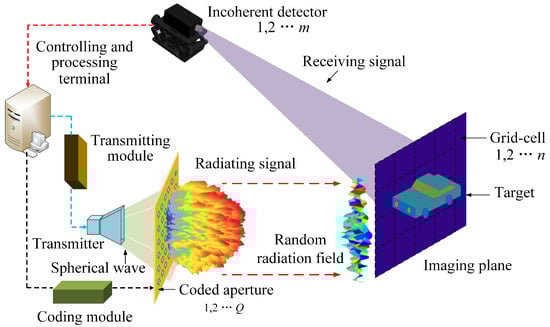
Figure 1.
Schematic of phaseless terahertz coded-aperture imaging (PL-TCAI) system.
2.2. Imaging Model
According to Figure 1, the imaging model of the PL-TCAI can be deduced in detail. Suppose the transmitter emits a THz linear frequency modulation (LFM) signal, which can be written as
where is the transmitting signal at time t, A is the amplitude, is the center frequency, K is the chirp rate. Then, the radiating signal of the -th sampleing can be deduced as
where is the scattering coefficient corresponding to the N-th grid cell, Q stands for the modulation elements of the coded aperture, and are the random amplitude modulation factors and phase modulation factors for the q-th coding aperture element at time respectively. For the amplitude modulation coded antenna, . For phase modulated coded antennas, , where ≡ stands for identity. The signal propagation distance is , where , , , represent the position vector of transmitter, the q-th elements of coded aperture, the N-th grid cell of imaging plane, and the incoherent detector, respectively. If the intensity detector samples the echo signal m times, the matrix imaging equation of PL-TCAI can be expressed as
where denotes the absolute value. is the target scattering coefficient vector, is the echo signal vector, and is the additive measurement noise. Thus, the imaging model can also be written concisely as
where is reference signal matrix, and can be expressed as
The row vector and column vector of are the time-domain samples at and the spatial-domain samples at respectively. Obviously, the imaging capability of PL-TCAI is affected by the structure of the reference signal matrix . In particular, each row of is affected by the coded-aperture modulation scheme, resulting in a random distribution of the row vector , . We can also observe that the scale of the reference signal matrix is large, mainly due to the short wavelength and precise resolving ability of THz waves make the imaging area divided into smaller grids. With the number of measurements increases, the scale of reference signal matrix is larger and the matrix imaging equation is more complex, which not only creates a heavy computation burden, but also greatly increases the hardware difficulty of echo signal detection. In addition, the detection of a large number of intensity signals will increase the times of coding and sampling, which will make it difficult to realize high-frame PL-TCAI imaging, and also not conducive to the design of the coded-antenna. Therefore, it is very necessary to study the algorithm of solving the target scattering coefficient under low measurement.
3. Target Reconstruction Principle and Imaging Algorithm
3.1. Target Reconstruction Principle
In the previous PL-TCAI [18,19], the solution of the target scattering coefficient is considered as an optimization problem after the estimation of the reference signal matrix is obtained.
where is L2 Norm, contains the prior knowledge on and is usually the variance of . Obviously, it is a non-deterministic polynomial hard (NP-hard) problem to solve the target scattering coefficient only from the intensity measurement . Although a large batch of theoretical analyses and numerical algorithms have been introduced to deal with the problem [18,19], these methods have encountered possibly fundamental limitations, they often fail to solve the target scattering coefficient when the intensity measurement m is less than n. To relieve the ill-posedness of the problem, we proposed a new framework for PL-TCAI.
In this work, as a prior, we assume the target of interest can be generated by a generative model . In particular, the generative model can be modeled as a d-layer, fully-connected, feed forward neural network with Rectifying Linear Unit (ReLU) activation functions and no bias terms. Let represent the weights of i-th layer of the network, where . When , then , , and . For and , ; When , then , , and . For and , . So the general expression for the generative model can be written as
where acts entrywise. We further suppose that each weight matrix has Gaussian entries, which is supported by the empirical evidence showing that the weights learned from the data obey statistics similar to Gaussian [29].
With the assumptions above, we know that the generative model can map a latent vector to a high dimensional sample space . Hence, we first recover the latent vector , and the mathematical formula can be expressed as
Then, can be obtained by applying the generative model G:
we refer to this approach as the deep gradient descent (Deep-GD) approach. In fact, the above equation usually exhibits highly non-convex behavior, which is very difficult to converge to global minimum. However, as mentioned above, a reference signal with benign geometrical structure can be obtained by selecting the appropriate coded- antenna modulation scheme, which is conducive for the PL-TCAI algorithm to find to a satisfactory solution.
3.2. Imaging Algorithm
Motivated by the study of phase recovery problem under Gaussian measurements Ref. [25,26,27], we designed Deep-GD algorithm for PL-TCAI, and the processing framework of the algorithm is shown in Figure 2. One can clearly see that the framework is actually an intuitive application of the idea of deep generative network to PL-TCAI tasks.
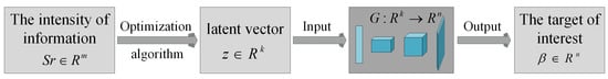
Figure 2.
The processing framework of Deep-GD algorithm.
As can be seen from Figure 2, the optimization of the latent vector is crucial to the reconstruction of the target. So we study the following L2 empirical risk minimization problem
Here, in order to calculate the gradient of descent at each step of the optimization algorithm, we assume generator G is differentiable and define to be a diagonal entry of the vector , and is 1 in the i-th diagonal entry if , and 0 otherwise. For and , define , which means keeps the rows of that have a positive dot product with . When , , then . Therefore, for any and , the derivative of the generative model can be written as
Moreover, with the assumptions above, , where is defined as sign for non-zero and otherwise. Therefore, the gradient in t-th iteration can be written as the following equation
where ⊙ stands for hadamar product and . We optimize over by gradient descent and perform the update until some convergence criteria are met. The learning rate is chosen empirically. Since all latent vectors are sampled uniformly from the hyper-cube, we project back to the bounded domain after each gradient update by using stochastic clipping
With this operation, we reassign the clipped components that are too large and too small at random in the allowed range. Also, [30] proves that the stochastic clipping technique facilitates precise recovery of the latent vector from generative adversarial networks. Algorithm 1 formally outlines this process.
| Algorithm 1: Deep Gradient Descent (Deep-GD) |
| Input: |
| Sb: echo signal intensities vector |
| S: reference signal martix |
| T: maximum iteration |
| G: generate network |
| Iteration via a gradient descent scheme: |
| 1: Initialize |
| 2: for t = 0 to T do |
| 3: Compute ; |
| 4: ; |
| 5: ; |
| 6: end for |
| 7: |
| Output: |
| the estimated target-scattering coefficient vector |
4. Numerical Tests
In this section, the feasibility of enforcing generative priors in PL-TCAI tasks is verified by numerical experiments. Parameters in the imaging system are given in Table 1. The frequency range of the THz signal is from 330 GHz to 350 GHz. The 1-bit transmission-type coded aperture has elements that are employed to modulate the phase of the transmitted signal by or , so . The imaging plane is divided into , and it is easy to calculate that the pixel interval is no larger than 0.007 m. To investigate the validity of the proposed algorithms, numerical experiments are carried out on sparse targets and extended targets respectively. The sparseness criteria proposed in [31] uses a measure based on the relationship between L1 and L2 norm of a given vector:
Obviously, the sparseness is 1 if and only if contains only a single non-zero component, and takes a value of 0 if and only if all components are equal, interpolating smoothly between the two extremes.

Table 1.
Parameters Used in the PL-TCAI Simulation Experiment.
According to the previous research [9], it is feasible to estimate the correlation between different rows and columns of the reference signal matrix to analyze the resolution of the imaging system. Therefore, the random radiation field distribution, spatial non-correlation and temporal non-correlation of the reference signal are investigated and the results are shown in Figure 3a–c respectively. It is clearly seen that the reference signal matrix has a benign geometric structure under the random phase modulation of the coded aperture, which will facilitate the phase recovery algorithm to converge to a satisfactory solution to achieve high-resolution imaging.
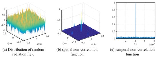
Figure 3.
Analysis of reference signal matrix.
In the simulation experiments, MNIST data set [32] and Fashion-MNIST data set [33] are selected as sparse target data set and extended target data set respectively, and both of them consist of 60,000 training images and 10,000 testing images. According to radar target characteristics, each image from MNIST and Fashion-MNIST data sets is resized to and is regarded as composed of scattered points, the corresponding scattering coefficient is a random value between zero and unity. In particular, these images from the adjusted data sets are viewed as targets. Subsequently, based on the terahertz coded-aperture imaging principle [9,13], the TCAI-MNIST data set and TCAI-FMNIST data set under the imaging parameters are generated through imaging algorithm. Generative models for TCAI-MNIST and TCAI-FMNIST follow the DCGAN [28] framework, and they were trained on a desktop computer with GPU NVIDIA 2080 and the CUDA edition is 9.0. The training took approximately 12 h, which is time-consuming. But this procedure can be done in advance. The Adam optimization algorithm is employed to optimize weights, and the learning is 0.0002. The batch size is 64 and the training lasts for 100 epochs. Two typical reconstruction algorithms for PL-TCAI, the WFOS algorithm and SWFOS algorithm, are chosen to compete with the presented approach, relative error, structural similarity (SSIM) and correlation coefficient are used as the quantitative index. Considering the small representation error, we tested 10 targets from the test set for each method to obtain a performance analysis curve except as specifically stated. The codes in this paper are implemented in Matlab and PyTorch. All reconstruction results were obtained on the computer with Inter Xeon Silver 4116 CPU except as specifically stated.
4.1. Results of Random Target on Fully-Connected Generator
We first consider synthetic experiments on a two-layer network given by , where . Let , . And the dimension of latent vector k is chosen from . We set the total number of iterations to , and the number of phaseless measurement m ranges from 20 to 1000 with interval 50. Under each m, the recovery rate is the percentage of successful times among 30 repeated tests with different initialization , and a recovery target is considered successful if the relative error in each test. The results are shown in Figure 4 and Table 2. As can be seen from Figure 4, the proposed method has a good performance to recover target under different intensity measurement. When , the recovery rates are not less than , and with the increase of measurement m, the recovery rates can be up to . Also, we find that the smaller k can have a higher recovery rate. Therefore, the value of latent vector k is crucial in the generative model. In particular, the sparseness and shape of the targets in each test are random, which indicates that the proposed method has good performance in the reconstruction of various targets. In addition, it can be found from Table 2 that the standard deviations are low, which fully demonstrates the stability of Deep-GD algorithm.
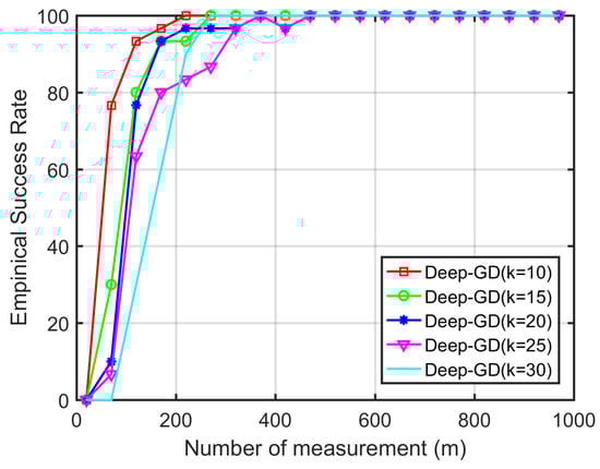
Figure 4.
Empirical success rate of Deep-GD at different measurements m under different k.
Table 2.
Average relative error and standard variation of reconstructions by using Deep-GD.
4.2. Results of Sparse Targets and Extended Targets on DCGAN
For our second experiments, the generative model follows the DCGAN framework that was trained on the TCAI-MNIST data set and also trained on TCAI-FMNIST data set. The latent vector dimension of DCGAN is . The learning rate and the number of iteration updates are set to 0.01 and 900 respectively. To investigate the validity of the presented algorithm, we first carried out simulation experiments at various targets, which are from TCAI-MNIST and TCAI-FMNIST test sets. The results are shown in Figure 5, and the sparseness of the original target is 0.6624, 0.7169, 0.6016, 0.6313, 0.6173, 0.4722, 0.5498, 0.5273, 0.5419, 0.4953, respectively. It can be seen that the proposed algorithm can recover not only sparse targets but also extended targets with intensity measurements, which is different from SWFOS algorithm [19] that can only recover the point scattering targets under low intensity measurement.
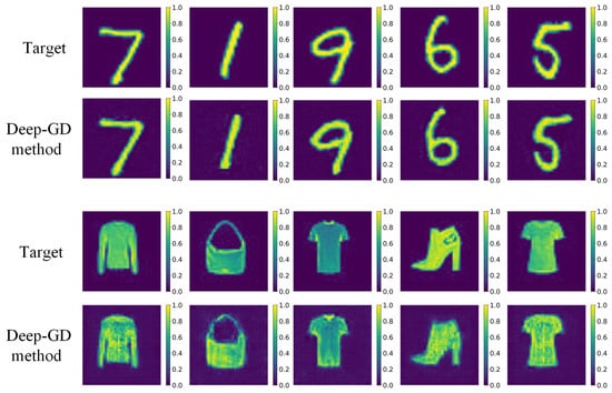
Figure 5.
Reconstruction results for different sparseness targets with measurements.
To further research the relationship between the recovery performance and intensity measurement, we next investigate sparse target and extended target recover tasks. For sparse target, we performed a simulation experiment with three different approaches on a generator trained over the TCAI-MNIST training dataset resized to pixel. Figure 6 shows the visualization results of the “1” whose scattering coefficients of all the point scatters are a value between zero and unity. One can clearly see that the object can be recovered through the generative model-based algorithm as low as while other methods cannot. With the increase of phaseless measurements m, the target can be perfectly reconstructed by using SWFOS and WFOS algorithms. However their performance degraded dramatically for lower values of m. In general, our method is competitive with the typical optimization iterative algorithms when m is not larger than n. In addition, motivated by [34], correlation is used to evaluate the reconstruction results of different methods under different intensity measurements. It can be seen from the results that the imaging performance of the proposed method is ultimately limited by the characterization error of the generative model. However, as can be seen in predicted target, the reconstructions are semantically correct.
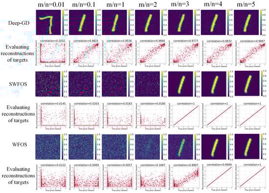
Figure 6.
Comparison of sparse target reconstruction results at different measurements.
Quantitatively, the relative error and SSIM comparisons under different measurements are described in Figure 7a,b, respectively. It can be seen that our algorithms can achieve good recovery with only 547 measurements while the other algorithms cannot, the relative error is below and SSIM is around 0.8. And both indexes can be improved slightly by increasing m with the similar phenomena with the results for fully-connected generator. But there are some oscillations, which can be attributed to the highly nonconvex property of DCGAN model and the property of the generative model. Also, we note that the imaging performance of the Deep-GD algorithm is ultimately bounded by the DCGAN’s representational error, which is consistent with the visualization shown in Figure 6. Nonetheless, our algorithm can solve the scattering coefficient of sparse targets under the intensity measurements m less than n.
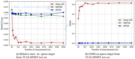
Figure 7.
Performance of sparse target under different measurements.
For extended targets, DCGAN trained on the TCAI-FMNIST data set is used as a generative model. The latent code dimension is and the size of the output is . Set and . The reconstruction results of three approaches under different measurements are displayed in Figure 8, where the sparseness of ground truth is 0.4722. We can find that the proposed algorithm can still have a good performance for extended target. In particular, since SWFOS algorithm is designed for sparse targets, it needs phaseless measurements to realize reconstruction of extended targets. Although WFOS algorithm is superior to SWFOS algorithm, it cannot reconstruct the target when . However, this Deep-GD method achieves 97.6% correlation versus the true target when . More evidences are shown in Figure 9. Again, we can clearly see the superiority of Deep-GD approach in reconstructing the extended target.
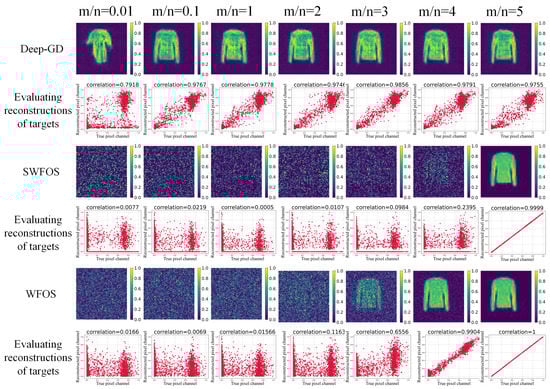
Figure 8.
Comparison of extended target reconstruction results at different measurements
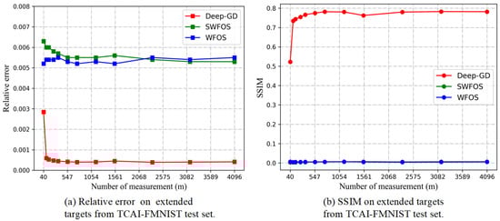
Figure 9.
Performance of extended target under different measurements.
To further evaluate the imaging performance of the proposed algorithm in the PL-TCAI system, we test 10 sparse targets from the test set of TCAI-MNIST data set and 10 extended targets from the test set of TCAI-FMNIST data set. The elapsed time of different methods on different targets is recorded, and the average results are shown in Table 3. In order to satisfy the successful reconstruction of all targets as far as possible, the number of detection data required for sparse target reconstruction is set as for SWFOS algorithm, for WFOS algorithm, and for Deep-GD algorithm, and the number of detection data required for extended target reconstruction is set as for SWFOS algorithm, for SWFOS algorithm, and for Deep-GD algorithm. From Table 3, we can see that the WFOS method and the Deep-GD method take about the same amount of time. But the neural network-based approach can be easily parallelized, so we also recorded the reconstruction time of Deep-GD algorithm with GPU implementation, which is far less than other algorithms. Therefore, the superiority of the imaging efficiency of the proposed method can be seen clearly.
Table 3.
Comparison on elapsed time for different methods.
5. Discussion
To examine the noise resistance and stability of the proposed Deep-GD method, we have added the white Gaussian noise to the echo signal. The quantitative and qualitative results are shown in Figure 10. The intensity measurement m is set to 500 and SNR = 20 dB. Figure 10a shows the reconstruction results of targets with different sparseness, and the sparseness of the original target is 0.5764, 0.5999, 0.6087, 0.587, 0.5937, 0.5065, respectively. For quantitative results, we test 10 sparse targets from the test set of TCAI-MNIST data set and 10 extended targets from the test set of TCAI-FMNIST data set, which is similar to the method used to analyze imaging efficiency. The average results are displayed in Figure 10b,c. One can see that the presented method is of good robustness against noise and a good stability at SNR > 10 dB when intensity measurement .
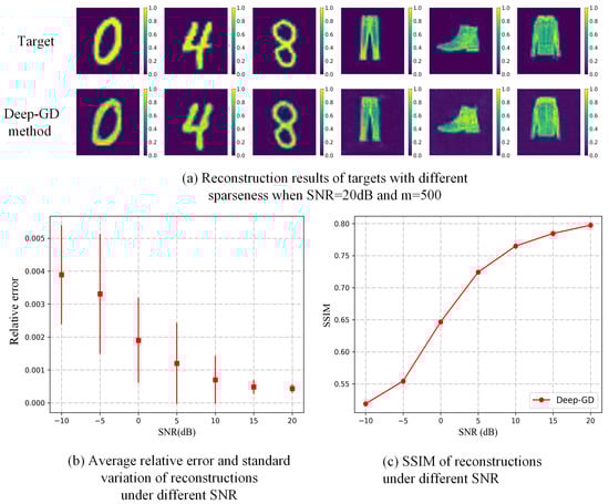
Figure 10.
Analysis of noise resistance and stability of the proposed Deep-GD method.
Compared with the classical imaging technology, the proposed method cannot reconstruct the targets that are not in the range of a generative model G as in [25,26,30], and its reconstruction results under high intensity measurements are not as perfect as other methods. However, it can use the prior information provided by the generative model to achieve the high-resolution reconstruction of targets with different sparseness when the intensity measurement , which greatly reduces the complexity of solving the target scattering coefficient and the difficulty of hardware required for the echo signal detection.
6. Conclusions
In this paper, a PL-TCAI algorithm based on generative model is presented. We first introduce the configuration of imaging system and the construction of imaging model. Subsequently, the principle of solving target scattering coefficient and Deep-GD algorithm are described in detail. Numerical tests based on fully-connected generator and DCGAN demonstrate the superiority of the proposed method, which can achieve a high recovery rate for targets with different sparseness when . Under this condition, classical PL-TCAI method nearly cannot recover the images. In addition, the proposed method has some advantages in imaging efficiency and robustness. With these advantages, the proposed method has a potential application in nondestructive detection, anti-terrorism checks, terminal guidance and so on. In further work, we intend to improve the performance of generate network and experimentally verify our method.
Author Contributions
Conceptualization, F.G.; methodology, F.G. and Z.Y.; software, F.G.; validation, F.G.; formal analysis, F.G. and Z.Y.; investigation, F.G. and C.L.; resources, C.L. and H.W.; data curation, F.G.; writing–original draft preparation, F.G.; writing—review and editing, Z.Y., H.W. and C.L.; visualization, F.G.; supervision, Z.Y., C.L. and H.W.; project administration, C.L. and H.W. All authors have read and agreed to the published version of the manuscript.
Funding
This research was funded by National Natural Science Foundation of China (NSFC) (61701513, 61971427, 61921001, 61871386).
Institutional Review Board Statement
Not applicable.
Informed Consent Statement
Not applicable.
Data Availability Statement
The data presented in this study are available on request from the corresponding author.
Conflicts of Interest
The authors declare no conflict of interest.
Abbreviations
The following abbreviations are used in this manuscript:
| PL-TCAI | Phaseless terahertz coded-aperture imaging |
| TCAI | Terahertz coded-aperture imaging |
| WF | Wirtinger Flow |
| TWF | Truncated Wirtinger Flow |
| WFOS | Wirtinger Flow with optimal stepsize |
| SWFOS | Sparse Wirtinger Flow alogithms with optimal stepsize |
| DCGAN | Deep convolutional generative adversarial networ |
| LFM | Linear frequency modulation |
| Deep-GD | Deep gradient descent |
| SSIM | structural similarity |
| TCAI-MNIST | Terahertz coded-aperture imaging MNIST |
| TCAI-FMNIST | Terahertz coded-aperture imaging Fashion-MNIST |
References
- Llull, P.; Liao, X.; Yuan, X.; Yang, J.; Kittle, D.; Carin, L.; Sapiro, G.; Brady, D.J. Coded aperture compressive temporal imaging. Opt. Express 2013, 21, 10526–10545. [Google Scholar] [CrossRef]
- Galvis, L.; Arguello, H.; Arce, G.R. Coded aperture design in mismatched compressive spectral imaging. Appl. Opt. 2015, 54, 9875. [Google Scholar] [CrossRef]
- Cheng, Y.Q.; Zhou, X.L.; Xu, X.; Qin, Y.L.; Wang, H.Q. Radar Coincidence Imaging with Stochastic Frequency Modulated Array. IEEE J. Sel. Top. Signal Process. 2016, 11, 414–427. [Google Scholar] [CrossRef]
- Li, D.Z.; Li, X.; Qin, Y.L.; Cheng, Y.Q.; Wang, H.Q. Radar Coincidence Imaging: An Instantaneous Imaging Technique with Stochastic Signals. IEEE Trans. Geosci. Remote Sens. 2014, 52, 2261–2277. [Google Scholar]
- Zhou, X.; Wang, H.; Cheng, Y.; Qin, Y.; Chen, H. Radar Coincidence Imaging for Off-Grid Target Using Frequency-Hopping Waveforms. Int. J. Antennas Propag. 2016. [Google Scholar] [CrossRef]
- Yin, Z.; Lu, Y.; Xia, T.; Lai, W.; Yang, J.; Lu, H.; Deng, G. Electrically tunable terahertz dual-band metamaterial absorber based on a liquid crystal. RSC Adv. 2018, 8, 4197–4203. [Google Scholar] [CrossRef]
- Perez-Palomino, G.; Barba, M.; Encinar, J.A.; Cahill, R.; Dickie, R.; Baine, P.; Bain, M. Design and Demonstration of an Electronically Scanned Reflectarray Antenna at 100 GHz Using Multiresonant Cells Based on Liquid Crystals. IEEE Trans. Antennas Propag. 2015, 63, 3722–3727. [Google Scholar] [CrossRef]
- Hunt, J.; Driscoll, T.; Mrozack, A.; Lipworth, G.; Reynolds, M.; Brady, D.; Smith, D.R. Metamaterial apertures for computational imaging. Science 2013, 339, 310–313. [Google Scholar] [CrossRef]
- Chen, S.; Luo, C.G.; Deng, B.; Qin, Y.L.; Wang, H.Q. Study on coding strategies for radar coded-aperture imaging in terahertz band. J. Electron. Imaging 2017, 26, 1. [Google Scholar] [CrossRef]
- Ullmann, I.; Adametz, J.; Oppelt, D.; Vossiek, M. Millimeter wave radar imaging for non-destructive detection of material defects. Proc. Sens. 2017, 2017, 467–472. [Google Scholar]
- Semenov, A.; Richter, H.; Böttger, U.; Hübers, H.W. Imaging terahertz radar for security applications. In Proceedings of the International Conference on Antennas, Radar and Wave Propagation, Baltimore, MD, USA, 16–18 April 2008. [Google Scholar]
- Luo, C.G.; Deng, B.; Wang, H.Q.; Qin, Y.L. High-resolution terahertz coded-aperture imaging for near-field three-dimensional target. Appl. Opt. 2019, 58, 3293–3300. [Google Scholar] [CrossRef]
- Chen, S.; Luo, C.G.; Wang, H.Q.; Deng, B.; Cheng, Y.Q.; Zhuang, Z. Three-Dimensional Terahertz Coded-Aperture Imaging Based on Matched Filtering and Convolutional Neural Network. Sensors 2018, 18, 1342. [Google Scholar] [CrossRef] [PubMed]
- Liu, X.; Luo, C.; Gan, F.; Wang, H.; Wang, Y. Antenna Phase Error Compensation for Terahertz Coded-Aperture Imaging. Electronics 2020, 9, 628. [Google Scholar] [CrossRef]
- Rogalski, A. Terahertz detectors and focal plane arrays. Elektronika 2010, 51, 93–108. [Google Scholar]
- Kawamura, J.; Tong, C.Y.E.; Blundell, R.; Papa, D.C.; Hunter, T.R.; Patt, F.; Gol’Tsman, G.; Gershenzon, E. Terahertz-frequency waveguide NbN hot-electron bolometer mixer. IEEE Trans. Appl. Supercond. 2001, 11, 952–954. [Google Scholar] [CrossRef]
- Yurduseven, O.; Fromenteze, T.; Smith, D.R. Relaxation of Alignment Errors and Phase Calibration in Computational Frequency-Diverse Imaging using Phase Retrieval. IEEE Access 2018, 6, 14884–14894. [Google Scholar] [CrossRef]
- Peng, L.; Luo, C.G.; Deng, B.; Wang, H.Q.; Qin, Y.L.; Chen, S. Phaseless Terahertz Coded-Aperture Imaging Based on Incoherent Detection. Sensors 2019, 19, 226. [Google Scholar] [CrossRef]
- Peng, L.; Luo, C.G.; Deng, B.; Wang, H.Q.; Chen, S.; Dong, J. Phaseless Terahertz Coded-Aperture Imaging for Sparse Target Based on Phase Retrieval Algorithm. Sensors 2019, 19, 4617. [Google Scholar] [CrossRef]
- Gerchberg, R.W. A practical algorithm for the determination of phase from image and diffraction plane pictures. Optik 1972, 35, 237–250. [Google Scholar]
- Candes, E.J.; Li, X.; Soltanolkotabi, M. Phase Retrieval via Wirtinger Flow: Theory and Algorithms. IEEE Trans. Inf. Theory 2015, 61, 1985–2007. [Google Scholar] [CrossRef]
- Chen, Y.; Candes, E.J. Solving Random Quadratic Systems of Equations Is Nearly as Easy as Solving Linear Systems. Commun. Pure Appl. Math. 2015, 70, 5. [Google Scholar] [CrossRef]
- Yuan, Z.Y.; Wang, H.X. Multiple Scattering Media Imaging via End-to-End Neural Network. arXiv 2018, arXiv:1806.09968. [Google Scholar]
- Rivenson, Y.; Zhang, Y.; Gunaydin, H.; Teng, D.; Ozcan, A. Phase recovery and holographic image reconstruction using deep learning in neural networks. Light Sci. Appl. 2017, 7, 17141. [Google Scholar] [CrossRef]
- Hyder, R.; Shah, V.; Hegde, C.; Asif, M.S. Alternating Phase Projected Gradient Descent with Generative Priors for Solving Compressive Phase Retrieval. In Proceedings of the ICASSP 2019—2019 IEEE International Conference on Acoustics, Speech and Signal Processing (ICASSP), Brighton, UK, 12–17 May 2019. [Google Scholar]
- YPaul, H.; Oscar, L.; Vladislav, V. Phase retrieval under a generative prior. In Proceedings of the Neural Information Processing Systems (NeurIPS), Montréal, QC, Canada, 3 December 2018. [Google Scholar]
- Shamshad, F.; Ahmed, A. Robust Compressive Phase Retrieval via Deep Generative Priors. arXiv 2018, arXiv:1808.05854. [Google Scholar]
- Radford, A.; Metz, L.; Chintala, S. Unsupervised Representation Learning with Deep Convolutional Generative Adversarial Networks. arXiv 2016, arXiv:1511.06434. [Google Scholar]
- Arora, S.; Liang, Y.; Ma, T. Why are deep nets reversible: A simple theory, with implications for training. arXiv 2015, arXiv:1511.05653. [Google Scholar]
- Lipton, Z.C.; Tripathi, S. Precise Recovery of Latent Vectors from Generative Adversarial Networks. arXiv 2017, arXiv:1702.04782. [Google Scholar]
- Hoyer, P.O. Nonnegative matrix factorization with sparseness constraints. J. Mach. Learn. Res. 2004, 5, 1457–1469. [Google Scholar]
- Lecun, Y.; Bottou, L. Gradient-based learning applied to document recognition. Proc. IEEE 1998, 86, 2278–2324. [Google Scholar] [CrossRef]
- Xiao, H.; Rasul, K.; Vollgraf, R. Fashion-MNIST: A Novel Image Dataset for Benchmarking Machine Learning Algorithms. arXiv 2017, arXiv:1708.07747. [Google Scholar]
- Bau, D.; Zhu, J.Y.; Wulff, J.; Peebles, W.; Strobelt, H.; Zhou, B.; Torralba, A. Seeing What a GAN Cannot Generate. In Proceedings of the IEEE International Conference on Computer Vision (ICCV), Seoul, Korea, 27 October–2 November 2019. [Google Scholar]
Publisher’s Note: MDPI stays neutral with regard to jurisdictional claims in published maps and institutional affiliations. |
© 2021 by the authors. Licensee MDPI, Basel, Switzerland. This article is an open access article distributed under the terms and conditions of the Creative Commons Attribution (CC BY) license (http://creativecommons.org/licenses/by/4.0/).