Evaluation of the Land GNSS-Reflected DDM Coherence on Soil Moisture Estimation from CYGNSS Data

Abstract

With the development of spaceborne global navigation satellite system-reflectometry (GNSS-R), it can be used for terrestrial applications as a promising remote sensing tool, such as soil moisture (SM) retrieval. The reflected L-band GNSS signal from the land surface can simultaneously generate coherent and incoherent scattering, depending on surface roughness. However, the contribution of the incoherent component was directly ignored in previous GNSS-R land soil moisture content retrieval due to the hypothesis of its relatively small proportion. In this paper, a detection method is proposed to distinguish the coherence of land GNSS-R delay-Doppler map (DDM) from the cyclone global navigation satellite system (CYGNSS) mission in terms of DDM power-spreading features, which are characterized by different classification estimators. The results show that the trailing edge slope of normalized integrated time-delay waveform presents a better performance to recognize coherent and incoherent dominated observations, indicating that 89.6% of CYGNSS land observations are dominated by the coherent component. Furthermore, the impact of the land GNSS-Reflected DDM coherence on soil moisture retrieval is evaluated from 19-month CYGNSS data. The experiment results show that the influence of incoherent component and incoherent observations is marginal for CYGNSS soil moisture retrieval, and the RMSE of GNSS-R derived soil moisture reaches 0.04 cm³/cm³.

1. Introduction

Soil moisture (SM) is an essential parameter for the hydrology and energy cycle. Rapid acquiring and accurate monitoring of terrestrial SM is not only required in the hydrological research but also a significant benefit to water management and agricultural production. Since the L-band microwave has a strong sensitivity to the change of surface SM and can more easily penetrate the atmosphere and vegetation canopy, it has been widely used as the main soil moisture remote sensing frequency band in the satellite-based radiometer and radar missions [1]. Such as the European Space Agency’s (ESA) Soil Moisture and Ocean Salinity (SMOS) mission and the National Aeronautics and Space Administration’s (NASA) Soil Moisture Active Passive (SMAP) mission, both can provide global SM measurement with the spatial resolution on the order of 40 km and coverage every 2–3 days using carried L-band radiometer. Spaceborne global navigation satellite system-reflectometry (GNSS-R) is an innovative and sustainable low-cost technique with high spatial and temporal resolution [2], which operates as a passive bistatic forward scattering radar. The observe system directly receives the pre-existing signals transmitted by the GNSS satellites reflected off the Earth’s surface [3], and the received scattering signals are typically expressed in a delay-Doppler map (DDM) for Earth’s surface geophysical parameters retrieval [4], which provide a new paradigm in the land remote sensing to cover the space-time gap of the traditional high-cost dedicated monostatic active or passive satellite missions.

In the past decade, spaceborne GNSS-R has undergone rapid development with successfully deployed satellite missions, such as the UK Technology Demonstration Satellite-1 (TDS-1, launched in July 2014), NASA’s cyclone global navigation satellite system (CYGNSS, launched in December 2016), China’s Bufeng-1 A/B mission (launched in June 2019) [5]. Although all missions were originally designed for ocean surface wind speed retrieval, they also provided a large number of land observations for terrestrial remote sensing applications, such as soil moisture retrieval, forest biomass estimation, and wetland extent detection [6]. However, there are many differences between GNSS-R land and ocean applications [7]. Before using GNSS-R for geophysical parameters retrieval, the key issue is to determine the scattering mechanisms of observed DDM. Over the sea surface, the surface height standard deviation is at least a significant fraction of the signal wavelength under windy conditions and increases with the wind speed [8,9], so the L-band GNSS signal echoes from the ocean are purely incoherent, which can be well explained by the Z-V model [10]. Compared to the ocean surface, the L-band signal scattering from the land surface is more complicated, and the GNSS signal returns are affected by many factors, such as soil moisture, vegetation, surface roughness, inland water, topographic relief, and soil texture. The DDM generated after noncoherent integration loses phase information, and the land surface small-scale roughness is variant in space and time, which is extremely difficult to be determined. As a result, it is hard to distinguish the coherence of land reflected DDM, which affects its subsequent land applications.

In previous GNSS-R land applications, it has been generally assumed that the coherent component dominates the land scattering field, and the incoherent component is negligible. The coherence defined here refers to reflected signals from the first Fresnel zone arriving at the GNSS-R receiver with similar phase shifts [9]. Many studies have proved that coherent DDM derived reflectivity is sensitive to the change of soil moisture and forest biomass [11,12,13,14,15]. However, due to the sensitivity of coherent and incoherent observation on the land geophysical parameters is different, it is important to distinguish the coherence of observations for quantified parameter retrieval. Theoretical simulations have revealed that the roughness of the land surface was close to 5 cm, where only incoherent scattering will occur [9]. Meanwhile, the effect of topography is independent of surface roughness, and the topographic relief can mitigate the reflectivity [16]. Different DDM observables have been used for GNSS-R sea ice detection based on the difference of coherent reflected signal from the sea ice surface and diffuse scattering from the sea surface [17,18]. However, it is relatively difficult to verify the coherence of current ground CYGNSS data. The coherence of a single complex DDM look can be robustly distinguished based on the differences of coherent and noncoherent integration from the “raw IF” signal [19] because the correlated power of a perfectly coherent signal will increase over the given period from longer integration lengths, while the incoherent will not. Unfortunately, the CYGNSS mission only recorded very few I/F signals limited by its storage capability. Nevertheless, with the help of these I/F signals from the land surface, different estimators have been characterized in the studies for DDM coherence detection [7,20], and the results show that the purely coherent reflection only occurs over the inland water surface in spaceborne GNSS-R observation. The problem is that the differences in estimator performance can lead to different results, and the I/F signal dataset used is too small, lacking sufficient persuasive power. Based on the different assumptions, several SM inversion methods have also been developed, such as spatial averaging, combine linear regression method, machine-learning method, and the global inversion accuracy of SM can reach about 0.05 cm³/cm³ [21,22,23,24,25,26,27,28,29,30].

In this paper, a statistical method is developed to detect the coherence of CYGNSS level-1 DDM from the land. We assume that the delay-Doppler-spreading features of incoherent DDM from the ocean and land scattering are similar, which all present a typical “horseshoe” shape, only the magnitude of the absolute scattering power differs. The defined estimators are used to determine the flag of coherence in terms of known incoherent DDM from the windy ocean surface, and the inversion accuracy of GNSS-R derived soil moisture with high confidence coherent DDM is evaluated and validated. The paper is organized as follows, Section 2 introduces the scattering theory over the sea surface and smooth soil surface and the definition of the coherent classification estimators based on the difference of typical coherent and incoherent dominated DDM. Section 3 shows the classification performance of different estimators, the distribution characteristics of coherent and incoherent observation over the land surface, and presents soil moisture retrieval results. Section 4 discusses the impact of coherent and incoherent DDM on SM remote sensing applications. Finally, conclusions are summarized in Section 5.

2. Methods and Datasets

If the land surface is relatively flat and smooth, the roughness of the scattering region is lower than the scale of the wavelength of the incoming GNSS signal; then the scattering mechanism is different from the diffuse scattering general occurring over the ocean surface. The land-coherent scattering only comes from the first Fresnel zone around the specular point instead of the whole glistening zone. The image theory and Friis transmission equation are used to explain this coherent forward scattering process, and the geophysical characteristics of the reflection surface are indicated by reflectivity [31]. As the surface roughness increases, the contribution of the incoherent component dramatically increases [32]; when the surface roughness approaches the signal wavelength scale, the conditions on the sea surface will recur. Next, we first introduce the scattering model, then present our coherence detection estimators, dataset, and GNSS-R soil moisture retrieval algorithm.

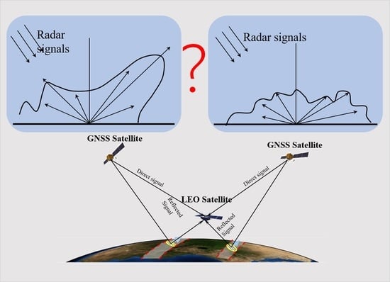
2.1. Bistatic Forward Scattering

The DDM is the function of signal time-delay and Doppler frequency shift from the surface specular point, which implies the mapping relationship of scattering power between space and delay-Doppler domain. When the L-band signal impinges on the rough sea surface, incoherent scattering occurs in most cases and scattering power can be well signified by the Z-V model [6]:

$$P(\widehat{\tau },{\widehat{f}}_D)=\frac{T_I^2{P}_T{\lambda }^2}{{(4\pi )}^3}{\displaystyle \underset{A}{\iint }\frac{G_T{\sigma }^0{G}_R}{R_R^2{R}_T^2}{\Lambda }^2(\widehat{\tau }-\tau ){\mathrm{sinc}}^2({\widehat{f}}_D-f_D)dA}$$

(1)

$$\chi (\widehat{\tau },{\widehat{f}}_D)=\Lambda (\widehat{\tau }-\tau )\mathrm{sinc}({\widehat{f}}_D-f_D)$$

(2)

$$\Lambda (\widehat{\tau }-\tau )=\left\{\begin{array}{l}{(1-\frac{\left|\widehat{\tau }-\tau \right|}{{\tau }_c})}^2\\ 0\end{array}\right.\begin{array}{c}\left|\widehat{\tau }-\tau \right|\le {\tau }_c\\ \left|\widehat{\tau }-\tau \right|>{\tau }_c\end{array}$$

(3)

$$\mathrm{sinc}({\widehat{f}}_D-f_D)={\left|\frac{\sin (\pi ({\widehat{f}}_D-f_D)T_I)}{\pi ({\widehat{f}}_D-f_D)T_I}\right|}^2$$

(4)

where $P(\widehat{\tau },{\widehat{f}}_D)$ is the complex, diffuse scattering power, $P_T$ is the right-hand circular polarized (RHCP) transmitted power of the GNSS satellite, $G_T$ is the transmitter antenna gain, $G_R$ is the GNSS-R receiver antenna gain, $R_R$ is the distance from the receiver to the scatter point over the ocean surface, $R_T$ is the distance from the transmitter to the scatter point, $\lambda$ is the wavelength of the GNSS carrier, $T_I$ is the coherent integration time, ${\sigma }^0$ is normalized bistatic radar cross-section, $\Lambda (\widehat{\tau }-\tau )$ is the correlation function of the GNSS navigation code, $\widehat{\tau }$ and $\tau$ are the local replica code in the receiver and received signal time delays, respectively, $\mathrm{sinc}({\widehat{f}}_D-f_D)$ is the attenuation due to Doppler misalignment, ${\widehat{f}}_D$ and $f_D$ are the local replica code in the receiver and received signal Doppler frequency shift, respectively. The product of the correlation function and the $\mathrm{sinc}$ function is called the Woodward ambiguity function (WAF) of the GNSS PRN navigation code. $A$ indicate the glistening zone, $dA$ is the differential area within the glistening zone. The ${\sigma }^0$ can be further expressed as:

$${\sigma }^0=\frac{\pi {\left|{\Re }_{LR}(\theta )\right|}^2{\overrightarrow{q}}^4}{q_z^4}P\left(-\frac{{\overrightarrow{q}}_{\perp }}{q_z}\right)$$

(5)

where ${\Re }_{LR}$ is the Fresnel reflection coefficient of scattered left-hand circular polarized (LHCP) signal over the sea surface, $\overrightarrow{q}$ is the scattering unit vector, ${\overrightarrow{q}}_{\perp }$ and $q_z$ are horizontal and vertical components, respectively, and $P$ is the probability density function of the sea surface slope. The coherent integration time commonly sets 1ms on the delay Doppler mapping instrument to generate a single DDM look. Due to the diffuse scattering signals over sea surface being relatively weak, to improve the signal-to-noise ratio (SNR) of DDM and reduce the effect of speckle and thermal noise within a coherent integration of a DDM look, there is an extra noncoherent integrated step that takes 1 s, during which the received signal will lose the phase information. Normalized bistatic radar cross-section (NBRCS) has been used as the land surface remote sensing fundamental observable in the backward scatterometer for a very long time, which is also reasonable to be employed in GNSS-R with specific calibration.

Theoretically, real land scattering power consists of coherent and incoherent components. After noncoherent integration, the DDM can be expressed as:

$$〈{\left|P(\widehat{\tau },{\widehat{f}}_D)\right|}^2〉=〈{\left|P_{coh}(\widehat{\tau },{\widehat{f}}_D)\right|}^2〉+〈{\left|P_{incoh}(\widehat{\tau },{\widehat{f}}_D)\right|}^2〉$$

(6)

where $〈{\left|P_{coh}(\widehat{\tau },{\widehat{f}}_D)\right|}^2〉$ and $〈{\left|P_{incoh}(\widehat{\tau },{\widehat{f}}_D)\right|}^2〉$ are coherent and incoherent contributions, respectively. Previous studies focus on land SM retrieval directly assumed that the incoherent item is negligible on Earth’s land surface; the received scattering power mainly concentrates from the adjacent region around specular point. According to the image theory and Friis transmission equation, the coherent scattering power coming from the first Fresnel zone can be expressed:

$$P_{coh}=\frac{P_T{G}_T{\lambda }^2{G}_R}{{(4\pi )}^2{(R_R+R_T)}^2}\Gamma (\theta ){\gamma }^2\exp (-{(2k\sigma \cos (\theta ))}^2)$$

(7)

where $\Gamma$ is reflectivity, it is the function of the Fresnel reflection coefficient $\Re$ ($\Gamma (\theta )={\left|{\Re }_{LR}(\theta )\right|}^2$). $\gamma$ is the transmissivity which indicates the vegetation layer attenuation, it is the function of vegetation opacity depth (VOD) $\tau$($\gamma =\exp (-\tau \sec \theta )$). The exponential term represents signal attenuation caused by surface roughness. $k$ is the wavenumber, and $\sigma$ represents the standard deviation of surface height. The size of the first Fresnel zone is related to the height of the receiver platform and signal incidence angle. For the CYGNSS mission, the diameter of the first Fresnel zone is about 0.5 km. Considering this small area compared to the spatial resolution of CYGNSS DDM pixels, it is reasonable to directly pick the peak power value in the DDM to calculate reflectivity. According to Equation (7), the surface reflectivity can be derived as follows:

$$\Gamma (\theta )=\frac{{(4\pi )}^2{P}_{peak}{(R_R+R_T)}^2}{{\lambda }^2{P}_T{G}_T{G}_R}$$

(8)

where $P_{peak}$ is the coherent power with surface roughness and vegetation attenuation correction. Since the velocity of CYGNSS satellites along the track is 7 km/s, the spatial resolution corresponding to the peak power measurement is about 0.5 km × 7 km. After June 2019, the sampling frequency of the CYGNSS mission has increased to 0.5 Hz, which allows the spatial resolution along the direction of satellite movement to reach 3.5 km.

When the roughness of the land surface is comparable to the scale of GNSS carrier wavelength, incoherent scattering will occur over the land surface. Since there is no reliable high spatial-temporal surface roughness information, it is difficult to determine the coherence of a DDM. The aforementioned assumption indeed ignores two issues for GNSS-R SM inversion. On one hand, if we directly consider that the main contribution of scattering power comes from the coherent component, which implies the influence of the incoherent components in DDM is ignored. On the other hand, when the GNSS-R observation footprint passes through the land surface with large roughness, the purely incoherent signal will be received, the influence of incoherent observations on the SM inversion is ignored as well. There is a big difference between the sensitivity of coherent and incoherent DDM observables to the SM level [9], so it is important to evaluate the influence of the previous assumption. Due to the different scattering mechanisms that happen behind the coherent and incoherent observations, the shape and magnitude of the measured scattering power in the DDM are different. The coherent DDM resembles the WAF itself without delay-doppler spreading [33]. Figure 1a shows a typical land reflected DDM over the winter wheat field. As a comparison, Figure 1b presents the DDM observed over the ocean surface with the 6.6 m/s wind speed near the specular point. The received diffuse scattering signals come from the entire glistening zone with the WAF spreading in the direction of delay and Doppler axis; DDM exhibits the typical “horseshoe” shape.

The time-delay waveform (DW) is the 1D representation of DDM; it is also a fundamental observable in the GNSS-R study, which usually includes two types: central Doppler time-delay waveform (CDW) and integrated time-delay waveform (IDW). The CDW is the zero Doppler delay scattering power in the DDM. The IDW is obtained by summing the columns along the Doppler axis of DDM. In our classification method, we also define the deviation of time-delay waveforms (DDW) calculated by IDW subtracting CDW at each time delay bin. It can be noticed from the land reflected DW in Figure 1c that the trailing edge scattering power quickly decreases to the noise floor level after the peak point, and the deviation between CDW and DDW is small. Whereas the scattering power of the trailing edge of DW derived from the sea surface scattered DDM decreases slowly, especially for IDW and DDW, which is shown in Figure 1d, and the peak and trailing edge power of DDW are much larger than CDW. As the land topography changes and the surface roughness increases, which can lead to the intensity of the incoherent field strengthened rapidly, the coherent field weakens according to the conservation of energy. Then, the magnitude and distribution characteristics of DDM gradually approach the sea surface observations. Based on these features, we proposed a method to classify CYGNSS coherent and incoherent observations.

2.2. Definition of Classification Estimator

Since the DDM observed from the ocean surface dominated by incoherent scattering and from the relatively flat land surface dominated by coherent scattering are significantly different [17,25], the coherence classification method proposed here is based on the shape and distribution characteristics of power-spreading in the DDM. Here and after, we directly call coherent component dominated DDM as coherent DDM, and incoherent component dominated as incoherent DDM. The whole classification idea is inspired by GNSS-R sea ice detection [17,18], and both are essentially determining the similarity to the coherent model. For the coherent DDM, it resembles the Woodward ambiguity function (WAF) without delay-doppler spreading [33], while incoherent DDM exhibits the typical “horseshoe” shape. The calculation of the defined classification estimators is introduced in the following part in detail. To characterizes the difference in the coherence of DDM, combining the known typical range of estimator values calculated from ocean scattered incoherent DDM, the threshold of coherence can be determined in the CYGNSS land observation. It should be noted that the reference position of defined DDM estimators from the land surface refers to the delay and doppler bin of the DDM peak power. If the DDM observable can be calculated from the DW, the selected window is set to spanning 5 time-delay bins from the peak. For the DDMA calculation, the selected delay/Doppler window is a 5 × 3 matrix with the center located on the peak location. The given window size mainly depends on two reasons. On one hand, the position of peak power is not fixed in each CYGNSS DDM, so when the entire DDM is directly used to calculate the estimator, the range of statistical delay and Doppler is different. On the other hand, it is based on the shape of WAF, which is shown in Figure 2. The main coherent reflection power concentrate on this zone. The final objective is to compute the probability density function (PDF) of DDM observables in the land and ocean observations to determine the separation threshold of coherent and incoherent dominated observations.

• TES: It is the trailing edge slope of the normalized DW and determined using the least-squares fitting within the time-delay window to a linear expression:

  $$a_{\mathrm{TES}}^N=\frac{n{\displaystyle \sum _{i=1}^n{\tau }_i{P}_i^N-}{\displaystyle \sum _{i=1}^n{\tau }_i{\displaystyle \sum _{i=1}^n{P}_i^N}}}{n{\displaystyle \sum _{i=1}^n{\tau }_i^2-{({\displaystyle \sum _{i=1}^n{\tau }_i})}^2}}$$

  (9)

  where n = 5 is the number of time-delay bins for the linear fitting. ${\tau }_i$ is the time-delay of each bin. $P_i^N$ is the normalized scattering power in raw count within the corresponding time-delay bin.
• TEV: It is the average volume of the normalized DW trailing edge:

  $${\overline{P}}_{\mathrm{TEV}}^N=\frac{1}{n}{\displaystyle \sum _{i=1}^n{P}_i^N}$$

  (10)
• TEV_POW: It is the average absolute scattering power of the DW trailing edge:

  $${\overline{P}}_{\mathrm{TEV}\_\mathrm{POW}}=\frac{1}{n}{\displaystyle \sum _{i=1}^n{P}_i}$$

  (11)

  where $P_i$ is the scattering power of the corresponding time-delay bin.
• DDMA: It is the average of the normalized scattering power DDM near its peak:

  $${\overline{\sigma }}_{\mathrm{DDMA}}^N=\frac{1}{nm}{\displaystyle \sum _{i=1}^n{\displaystyle \sum _{j=1}^m{P}_{i,j}^N}}$$

  (12)

  where $n$ and $m$ indicate the selected size of delay and Doppler window.
• DDMA_POW: It is the average of the absolute scattering power DDM near the peak:

  $${\overline{\sigma }}_{\mathrm{DDMA}\_\mathrm{POW}}=\frac{1}{mn}{\displaystyle \sum _{i=1}^n{\displaystyle \sum _{j=1}^m{P}_{i,j}}}$$

  (13)
• MF: It is known as the WAF-matched filter (MF) approach, which directly calculates the correlation coefficient of normalized DDM and unitary energy WAF:

  $$R_{\mathrm{MF}}=\frac{{\left|〈〈{\left|P(\widehat{\tau },{\widehat{f}}_D)\right|}^2〉,\chi (\widehat{\tau },{\widehat{f}}_D)〉\right|}^2}{〈〈{\left|P(\widehat{\tau },{\widehat{f}}_D)\right|}^2〉,〈{\left|P(\widehat{\tau },{\widehat{f}}_D)\right|}^2〉〉〈\chi (\widehat{\tau },{\widehat{f}}_D),\chi (\widehat{\tau },{\widehat{f}}_D)〉}$$

  (14)

2.3. Dataset for Soil Moisture Retrieval

CYGNSS is part of the NASA Earth system science pathfinder program; it is deployed as the first dedicated spaceborne GNSS-R constellation launched in December 2016. The space segment consists of eight microsatellites orbiting on a non-synchronous near-circular orbit with an inclination of approximately 35° (all spacecraft distributed on the same orbital plane). Each spacecraft is capable of tracking 4 reflections simultaneously, resulting in 32 DDMs per second over the Earth’s surface. The standard CYGNSS DDM consists of 17 delay bins with the resolution of a quarter of the GPS C/A chip by 11 Doppler bins with an interval of 500 Hz. Each DDM was processed using 1 ms coherent integration followed by 1000 looks of noncoherent averaging. After July 2019, the noncoherent time was reduced to 0.5 s. The primary objective of CYGNSS is to monitor the wind speed during the evolution of tropical cyclones. The footprint of its measurement covers the critical latitude band between ±38° [34]. At the same time, it also provides substantial land observations within this scope. The work conducting in this paper uses the CYGNSS level-1 DDMs in power analog from published version 2.1 data product ranging from January 2018 to August 2019. General data quality control (QC) in the land application is also utilized, the DDM SNR lower than 2 dB, receiver antenna gain at the specular point direction lower than 0 dB, and specular incidence angle over 65° are screened. To get the purely incoherent DDMs from the ocean surface [9], the corresponding DDMs with ERA5 wind speed greater than 5 m/s are employed. Land and sea surface observations are directly distinguished by the quality flag provided in the CYGNSS level-1 data.

The SMAP dataset used as the land surface reference SM is version 6 level-3 radiometer global daily 36 km equal-area scalable earth grid version 2.0 (EASE-Grid 2.0) soil moisture product within the same period time of the CYGNSS dataset [35], except the data product missing from 20 June to 22 July 2019. The SMAP SM data provides daily descending (a.m.) and ascending passes (p.m.) measurement, including the auxiliary parameters VOD (in the SMAP product indicates vegetation opacity parameter) and surface roughness coefficient (in the SMAP product indicates vegetation_roughness_coefficient), which are used to correct the attenuation of CYGNSS scattering power from the impact of surface roughness and vegetation canopy. In the soil moisture retrieval process, only the recommended data are used without the open water, urban area.

2.4. Soil Moisture Retrieval Algorithm

In previous spaceborne GNSS-R soil moisture retrieval studies, the primary methodology is to establish the relationship between GNSS-R derived land surface reflectivity and reference truth SM values, which assumes that coherent component dominates GNSS-R land scattering field. In the theory of surface electromagnetic scattering, the surface reflectivity is the function of the incidence angle of the incoming signal and the Fresnel reflection coefficient; the latter one is mainly affected by the near-surface SM [1]. Figure 3 simulates the relationship between reflectivity and SM at different incidence angles with the solid line, where the semi-empirical Dobson model is used to mapping the relationship between soil moisture and complex permittivity [36]. The surface reflectivity increases monotonously with soil becoming wetter, and the response of reflectivity to the change of SM from 0.0 cm³/cm³ to 0.7 cm³/cm³ can reach 10 dB. The effect of the incidence angle on the mapping relationship between SM and reflectivity is negligible when the incidence angle is less than 60°. In our CYGNSS SM inversion experiements, the DDM peak value of coherent scattered power is picked in the CYGNSS level-1 data as the left term of Equation (7). Since the small scale roughness and upwelling vegetation cover can attenuate the scattering signal, the roughness and vegetation correction in Equation (7) directly use the roughness coefficient and VOD parameter provided in SMAP product for individual observation. Although the influence of the signal incidence angle is small, the method proposed in [25] is still used in this work. The effect of the incidence angle correction is represented by the dashed lines in Figure 3 as well.

Due to the pseudorandom distribution of CYGNSS measurement, the influence of observation noise, and the spatial difference of surface roughness and vegetation cover at the specular point, currently, it is difficult to directly establish a reliable SM retrieval model at the GNSS-R specular point modeling all these factors, the optimal approach is to improve the SNR of reflectivity using the space–time-averaging method to form the gridded retrieval model [18]. Since the SM reference data used in this work is from the SMAP level-3 version 6 product, the individual CYGNSS reflectivity calculated with Equation (8) within one day will be projected into a global cylindrical 36 km × 36 km EASE-Grid 2.0 grid to align with the reference SM values, the average reflectivity is picked as the grid value. Here, we set a data quality control criterion; if the count of projected reflectivity at the grid is less than three, the corresponding grid observation will be considered invalid on that day. Next, the time matching is used to combine the gridded reflectivity and SMAP SM to establish the training dataset and mask the pixels in the SMAP SM data flagged with inland water and urban areas. Finally, the retrieval model is fitted at each grid. Usually, the variation range of local surface soil moisture is limited in a year; the linear model can achieve high modeling accuracy. Therefore, the training samples are used to fit the linear model between mean reflectivity and reference SM values pixel-by-pixel:

$$\mathrm{S}{\mathrm{M}}_{i,j}^{CYGNSS}=a_{i,j}{\overline{\Gamma }}_{i,j}+b_{i,j}$$

(15)

where the $a$ and $b$ are the pending parameters of the model. $i$ and $j$ are the grid location in the 36 km × 36 km EASE-Grid 2.0 grid. $\overline{\Gamma }$ is the grid mean reflectivity after space-time average processing.

3. Results and Analysis

3.1. Performance Evaluation of DDM Observables

In this work, we assume that coherent and incoherent scattering simultaneously occurs on the land surface in the CYGNSS land observations, and only two scattering cases appear: coherent reflection mainly contributed to DDM or incoherent scattering mainly contributed to DDM. We classify the two cases based on the statistical characteristics of the predefined estimators. Since we have known that ocean surface observation belongs to the latter, the characteristic information of incoherent DDM can be obtained. To evaluate the performance of different classification estimators defined in Section 2.2, the CYGNSS collected land and ocean DDMs in January 2018 are used to calculate the PDF and accumulation distribution function (CDF) of each DDM observable separately. Figure 4 gives the PDF and CDF of TES, TEV, TEV_POW calculated from CDW (top row), IDW (middle row), and DDW (bottom row). It can be found that the performance of the three types of DW-derived classification estimators is different. The PDF of TES between land and ocean observations is separated more and sharper, which means that the classification results of TES are generally better than the other two. TES values from ocean surface scattered signals are generally larger than land observation; its PDF appears on the right side of the figure. The reason is the L-band GNSS signals impinge on the ocean surface always occurring diffuse scattering, the time-delay, and Doppler-spreading cause DW to appear a significant “smearing” feature; in other words, the scattered power of the trailing edge will slowly decrease. In addition, the PDF of land reflected DDM-derived TES is more dispersed than ocean observations. In the first column of Figure 4, the closer TES to the left side of the x-axis, the greater the contribution of the coherent component to the DDM since the DW is much closer to the WAF correlation function. As the roughness of the land surface increases, the contribution of the incoherent component rapidly increases and begins to impact the scattering power of the DW trailing edge, so the TES value gradually approaches the ocean observations, two PDFs finally intersect. The performance of TEV_POW is the worst; the distribution of PDF from the land and ocean observations is overlapped. It can be explained by the fact that the peak value of coherent DM is larger than incoherent DM, while the scattering power of incoherent DW declines slowly after the peak value, the final result is the average of absolute scattering power within 5 time-delay bins between land and ocean DDM derived TEV_POW are close. The performance of TEV is in the middle.

Figure 5 shows the PDF of estimator DDMA, DDMA_POW, and MF derived from the ocean and land DDMs. The performance of DDMA_POW is very close to TEV_POW; the distribution of two PDF almost overlaps, which can be explained by the same reason as TEV_POW. Therefore, we can conclude that it is difficult to determine the coherence of the DDM based on the feature of its absolute power in the given window. In the rest of the paper, we will exclude the absolute power estimators. Here, MF shows the best performance; DDM from land generally has a higher correlation with the WAF in comparison with the ocean, which is in line with the previous assumption.

The performance of different estimators is variant depending on the land surface scattering mechanisms; the classification threshold is determined by the intersection of two PDFs, which is represented by the magenta dotted line in the vertical direction in Figure 4 and Figure 5. The horizontal magenta dotted lines indicate the accumulative probability density of the corresponding estimator computed from the CYGNSS land and ocean surface data, which not only presents the probability of detection (PD) of coherent DDM but also indicates the proportion of the coherent and incoherent data.

Table 1. The classification threshold and the probability of different DDM observables.

Observables	${\mathit{a}}_{\mathrm{TES}}^{\mathit{N},\mathrm{CDW}}$	${\overline{\mathit{P}}}_{\mathrm{TEV}}^{\mathit{N},\mathrm{CDW}}$	${\mathit{a}}_{\mathrm{TES}}^{\mathit{N},\mathrm{IDW}}$	${\overline{\mathit{P}}}_{\mathrm{TEV}}^{\mathit{N},\mathrm{IDW}}$	${\mathit{a}}_{\mathrm{TES}}^{\mathit{N},\mathrm{DDW}}$	${\overline{\mathit{P}}}_{\mathrm{TEV}}^{\mathit{N},\mathrm{DDW}}$	${\overline{\mathit{\sigma }}}_{\mathrm{DDMA}}^{\mathit{N}}$	${\mathit{R}}_{\mathrm{MF}}$
Threshold	−0.6191	0.6878	−0.1798	0.8726	−0.0394	0.8144	0.7053	0.6171
PD	0.9146	0.8789	0.9379	0.9132	0.9192	0.7307	0.9368	0.9362
PFA	0.0284	0.0360	0.0289	0.0376	0.0312	0.0808	0.0310	0.0381
PE	0.0569	0.0786	0.0455	0.0622	0.0560	0.1751	0.0471	0.0510

summarizes the classification threshold, PD, the probability of false alarm (PFA), and the probability of error (PE) of each estimator. It can be found that the PD between different observables is small except DDW-derived TEV, and the average PD of all estimators is 89.6%. Among eight estimators, the PD of TES calculated from normalized IDW (NIDW) is the largest, and the PE is the smallest. Comparing all the subgraphs in Figure 4, it can also be found that the PDF of NIDW-derived TES is more separated between land and ocean data. Moreover, it is more concentrated and sharper than normalized CDW, and normalized DDW derived TES. Hence, it is considered the best estimator to detect the coherent and incoherent DDM collected over the land surface in this study. In the rest of the paper, we just use NIDW-derived TES as the classification estimator to recognize the high confidence coherent DDM in the CYGNSS land data for SM retrieval.

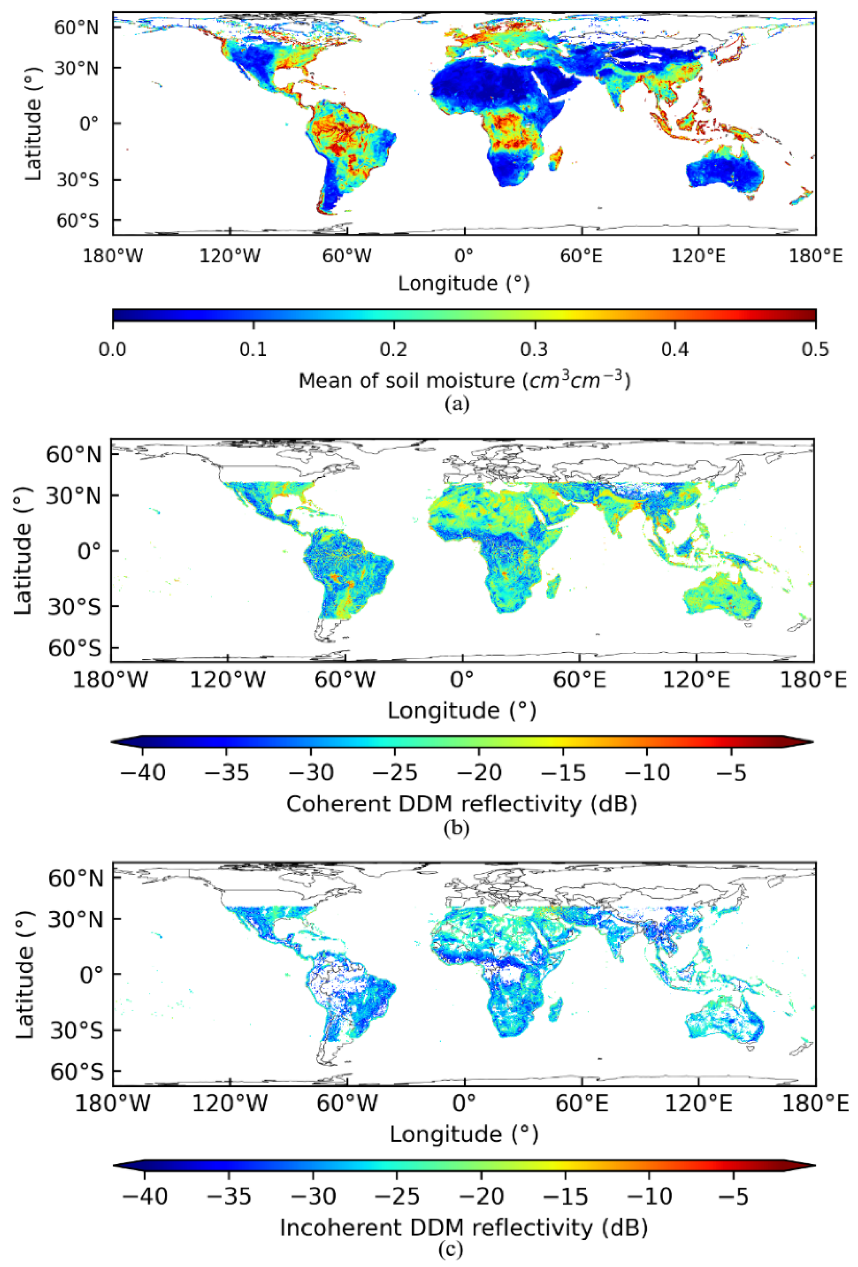
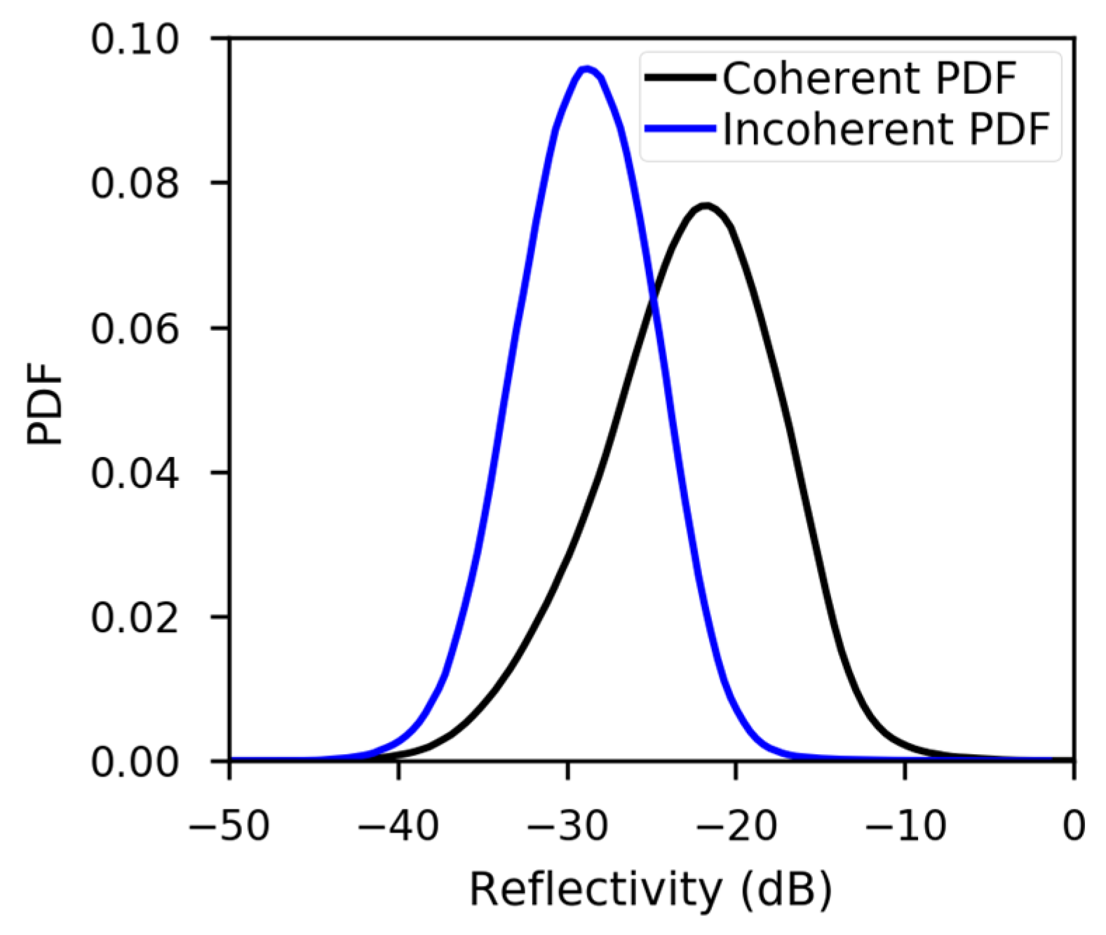
3.2. Coherent and Incoherent DDM Observations

The coherent and incoherent observation is determined by the threshold of the classification estimator of NIDW-derived TES. Figure 6 shows the average SM values from 9 km EASE-Grid 2.0 SMAP level-3 product, average CYGNSS gridded coherent and incoherent land surface reflectivity with the same projection grid in January 2018. Land coherent DDM can be detected in the entire footprint of the CYGNSS mission, whereas incoherent observations are more likely to occur in high altitude mountainous and hilly terrain.

According to the classification results, the range of coherent reflectivity is from −44 dB to −3 dB; the strongest coherent reflection indeed comes from the inland open water surface, while the area of the tropical rainforest and the arid mountainous area has the lowest reflectivity. It is worthy to note that the GNSS-R reflectivity over tropical dense forest areas is lower than the barren/desert area, which is consistent with previous studies [37]. Nevertheless, compared to the distribution of SMAP SM in Figure 6a, it can be found that the SM values in corresponding areas are high. Meanwhile, incoherent scattering rarely occurs in dense vegetation-covered areas, as Figure 6c shown. However, part of the reason is the applying of QC, which excludes some noisy DDM with lower DDN SNR. However, even we ignore the influence of QC, the count of involved incoherent observations for spatial averaging is still less than four in most of the grids, which is much smaller than the total number of coherent measurements in the same grid. In terms of the International Geosphere-Biosphere Program (IGBP) land cover type parameters provided in the SMAP products, the statistical results also show that the proportion of coherent and incoherent GNSS-R observations over different land cover types is almost the same before and after QC. It confirms that even the dense upwelling vegetation cannot change the scattering mechanism of the land surface, but dense forest canopies will generate a strong attenuation effect on the GNSS-R coherent scattering signals, which may be attributed to vegetation volume scattering. Moreover, many coherent and incoherent overlapped areas can be found in Figure 6b,c; we speculate that the main reason is the spatial distribution of the surface roughness is different within the projected grid, so the coherent and incoherent observations can be collected simultaneously in a grid.

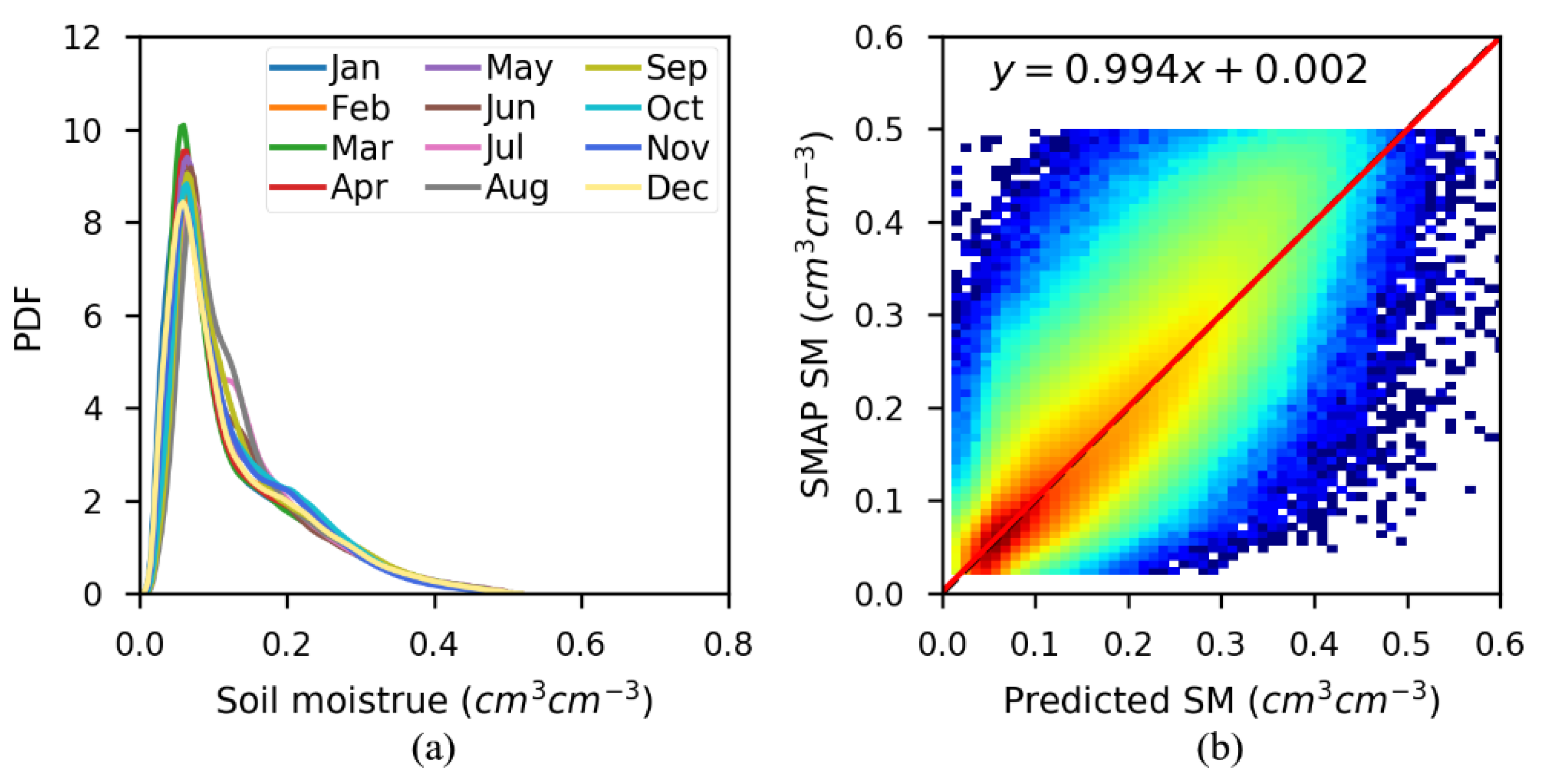
3.3. GNSS-R Soil Moisture Retrieval

To analyze the influence of incoherent observations on the GNSS-R land surface SM inversion in the previous SM retrieval method, we compared two retrieval configurations: using 19 months CYGNSS land observations and screened coherent data for retrieval model evaluation with k-fold cross-validation approach, where k = 5. Since the global SM value in most areas of the land is generally small in a year, the PDF of the monthly SMAP SM data in 2018 is presented in Figure 7a, and the maximum probability density of SM is 0.06 cm³/cm³. To further evaluate the performance of the established SM model over the high-humidity areas, the accuracy of the inversion model is evaluated when the referenced SM value is greater than 0.1 cm³/cm³.

Using the SM inversion method introduced in Section 2.4,

Table 2. Soil moisture retrieval model evaluating with k-fold cross-validation (unit: cm³/cm³).

Dataset	Total Bias	Total MAE	Total RMSE	SM > 0.1, Bias	SM > 0.1, MAE	SM > 0.1, RMSE
All land observations	−0.0003	0.0274	0.0416	−0.0124	0.0426	0.0569
Coherent observations	−0.0003	0.0269	0.0408	−0.0123	0.0421	0.0564

summarizes the performance of the two models established from two training datasets. When all CYGNSS land observations are used for modeling, the cross-validation model bias, mean absolute error (MAE) and root-mean-square error (RMSE) are −0.0003 cm³/cm³, 0.0274 cm³/cm³, and 0.0416 cm³/cm³, respectively. The inversion results with the distinguished coherent observation training dataset constructed retrieval model show that the bias, MAE, and RMSE are −0.0003 cm³/cm³, 0.0269 cm³/cm³, and 0.0408 cm³/cm³, respectively. The model performance between the two strategies is very close. When the SM reference values are greater than 0.1 cm³/cm³, the model accuracy of the two methods is 0.0569 cm³/cm³ and 0.0564 cm³/cm³, respectively, and the inversion results did not show a big difference. Figure 7b shows the density scatterplot between SMAP reference SM and GNSS-R-derived SM generated from a split of k-fold cross-validation with the coherent observation established model. The red line represents the linear fitting line; the predicted SM shows an overall fairly good agreement with the SMAP SM, all CYGNSS land data retrieved SM show an identical situation. Figure 8 presents the coherent inversion accuracy at each grid pixel with k-fold cross-validation. The analysis shows that CYGNSS incoherent observations will not cause any noticeable SM spatial inversion accuracy differences compared to the coherent results, so it is not given here.

4. Discussion

GNSS-R coherent and incoherent observations have different sensitivities to the land SM values [9]. According to the classification results with the defined estimator in this study, 6.2% of the measurements in the CYGNSS land observations have a high possibility controlled by the incoherent scattering field. In addition, the PDFs of reflectivity calculated from the land surface coherent and incoherent observations do show distribution differences, as shown in Figure 9. It should be noted that if the DDM scattering power is dominated by incoherent components, NBRCS is commonly picked as the fundamental quantity, which is calculated according to [21]. Since most of the previous studies ignored incoherent scattering, namely the counterpart reflectivity is directly calculated by Equation (8), it is reasonable to use this equation to calculate incoherent reflectivity and analyze their influence on CYGNSS SM retrieval in this paper. The experiments show that extra incoherent observations have no obvious effect on the final CYGNSS SM retrieval with space-time averaging combined with the linear regression method. To further validate this conclusion, the threshold of NIDW-derived TES is set to −0.5 to improve the confidence of discriminated coherent DDM, where the probability of false alarm is only 0.01. It also can be considered that the contribution of the incoherent component is very small in screened coherent observations. At this point, the coherent DDM accounts for 75.8% of CYGNSS land measurements. The bias, MAE, and RMSE of final inversed soil moisture are −0.0003 cm³/cm³, 0.0265 cm³/cm³, and 0.0403 cm³/cm³, respectively. The RMSE is reduced by 3.1% compared to the constructed model with assuming all coherent land observations. When the reference SM value is greater than 0.1 cm³/cm³, the inversion bias is −0.0145 cm³/cm³, MAE values is 0.0416 cm³/cm³, and RMSE is 0.0558 cm³/cm³.

The inversion accuracy of the aforementioned GNSS-R space-time averaging SM retrieval methods with two different training datasets is similar because the magnitude and number of incoherent reflectivity are smaller when compared to coherent reflectivity, and the spatial average processing will further mitigate its influence. However, there is no doubt that coherence classification methods play a key role in future GNSS-R land detection. The inversion model can be directly established at the individual specular point with improved high-quality and high spatial resolution observations, which provides in the following dedicated spaceborne GNSS-R land remote sensing missions, and also contributes to other land applications, such as inland water system detection, biomass detection, and wetland extent determination. Another noteworthy issue is that the established GNSS-R SM inversion model tends to underestimate the surface soil moisture when the land SM over 0.3 cm³/cm³, while most of the previous studies also show the same problem. Since most training samples are concentrated in the lower SM range, the regression model is more affected by this part of the data. Therefore, there should be a better weighting strategy to solve this problem in future work.

5. Conclusions

This paper presents a classification methodology to distinguish coherent and incoherent DDMs in the CYGNSS land observations. Since the GNSS scattering signals from the windy ocean surface are almost incoherent, while the coherent land DDMs are closer to WAF, six different classification estimators are established based on scattering power-spreading shape and magnitude features over the ocean, and land CYGNSS collected DDMs, which are used to screen the land high confidence coherent component dominated DDMs. The results show that the estimators based on the absolute magnitude features of DDM are difficult to distinguish its coherency, while the estimator indicating shape features performs better. The average proportion of GNSS-R land observations dominated by coherent components is 89.6%. NIDW-derived TES performs best among all defined DDM observables, and its PDFs from the ocean and land DDMs are more separated and sharper, whose detection probability for coherent observations can reach 93.8% with the lowest detection probability of error. The distribution of high-confidence coherent and incoherent surface observation indicates that observations over the dense forest cannot change the surface scattering properties but will greatly weaken the coherent scattering power. Using 19 months of CYGNSS observation data and SMAP SM product for land SM retrieval model validation, the RMSE of model performance with k-fold cross-validation can reach 0.04 cm³/cm³. Incoherent observations have not seriously impaired the accuracy of CYGNSS soil moisture inversion.

References

1. Njoku, E.G.; Entekhabi, D. Passive microwave remote sensing of soil moisture. J. Hydrol. 1996, 184, 101–129. [Google Scholar] [CrossRef]
2. Jin, S.; Feng, G.P.; Gleason, S. Remote sensing using GNSS signals: Current status and future directions. Adv. Space Res. 2011, 47, 1645–1653. [Google Scholar] [CrossRef]
3. Ruf, C.S.; Chew, C.; Lang, T.; Morris, M.G.; Nave, K.; Ridley, A.; Balasubramaniam, R. A New Paradigm in Earth Environmental Monitoring with the CYGNSS Small Satellite Constellation. Sci. Rep. 2018, 8, 8782. [Google Scholar] [CrossRef] [PubMed] [Green Version]
4. Jin, S.; Zhang, Q.; Qian, X. New progress and application prospects of global navigation satellite system reflectometry (GNSS+ R). Acta Geod. Cartogr. Sin. 2017, 46, 1389–1398. [Google Scholar]
5. Jing, C.; Niu, X.; Duan, C.; Lu, F.; Di, G.; Yang, X. Sea Surface Wind Speed Retrieval from the First Chinese GNSS-R Mission: Technique and Preliminary Results. Remote Sens. 2019, 11, 3013. [Google Scholar] [CrossRef] [Green Version]
6. Zavorotny, V.U.; Gleason, S.; Cardellach, E.; Camps, A. Tutorial on Remote Sensing Using GNSS Bistatic Radar of Opportunity. IEEE Geosci. Remote Sens. Mag. 2014, 2, 8–45. [Google Scholar] [CrossRef] [Green Version]
7. Gleason, S.; O’Brien, A.; Russel, A.; Al-Khaldi, M.M.; Johnson, J.T. Geolocation, Calibration and Surface Resolution of CYGNSS GNSS-R Land Observations. Remote Sens. 2020, 12, 1317. [Google Scholar] [CrossRef] [Green Version]
8. Comite, D.; Ticconi, F.; Dente, L.; Guerriero, L.; Pierdicca, N. Bistatic Coherent Scattering From Rough Soils With Application to GNSS Reflectometry. IEEE Trans. Geosci. Remote Sens. 2019, 1–14. [Google Scholar] [CrossRef]
9. Balakhder, A.M.; Al-Khaldi, M.M.; Johnson, J.T. On the Coherency of Ocean and Land Surface Specular Scattering for GNSS-R and Signals of Opportunity Systems. IEEE Trans. Geosci. Remote Sens. 2019, 1–11. [Google Scholar] [CrossRef]
10. Zavorotny, V.U.; Voronovich, A.G. Scattering of GPS signals from the ocean with wind remote sensing application. IEEE Trans. Geosci. Remote Sens. 2000, 38, 951–964. [Google Scholar] [CrossRef] [Green Version]
11. Chew, C.; Shah, R.; Zuffada, C.; Hajj, G.; Masters, D.; Mannucci, A.J. Demonstrating soil moisture remote sensing with observations from the UK TechDemoSat-1 satellite mission. Geophys. Res. Lett. 2016, 43, 3317–3324. [Google Scholar] [CrossRef] [Green Version]
12. Camps, A.; Park, H.; Pablos, M.; Foti, G.; Gommenginger, C.P.; Liu, P.W.; Judge, J. Sensitivity of GNSS-R Space-borne observations to soil moisture and vagetation. IEEE J. Sel. Top. Appl. Earth Obs. Remote Sens. 2016, 9, 4730–4742. [Google Scholar] [CrossRef] [Green Version]
13. Camps, A.; Llossera, M.V.; Park, H.; Portal, G.; Rossato, L. Sensitivity of TDS-1 GNSS-R Reflectivity to Soil Moisture: Global and Regional Differences and Impact of Different Spatial Scales. Remote Sens. 2018, 10, 1856. [Google Scholar] [CrossRef] [Green Version]
14. Zribi, M.; Guyon, D.; Motte, E.; Dayau, S.; Wigneron, J.P.; Baghdadi, N.; Pierdicca, N. Performance of GNSS-R GLORI data for biomass estimation over the Landes forest. Int. J. Appl. Earth Obs. Geoinf. 2019, 74, 150–158. [Google Scholar] [CrossRef]
15. Carreno-Luengo, H.; Luzi, G.; Crosetto, M. Biomass Estimation Over Tropical Rainforests Using GNSS-R On-Board The CyGNSS Microsatellites Constellation. In Proceedings of the IGARSS 2019–2019 IEEE International Geoscience and Remote Sensing Symposium, Yokohama, Japan, 28 July–2 August 2019; pp. 8676–8679. [Google Scholar]
16. Dente, L.; Guerriero, L.; Comite, D.; Pierdicca, N. Space-Borne GNSS-R Signal Over a Complex Topography: Modeling and Validation. IEEE J. Sel. Top. Appl. Earth Obs. Remote Sens. 2020, 13, 1218–1233. [Google Scholar] [CrossRef]
17. Alonso-Arroyo, A.; Zavorotny, V.U.; Camps, A. Sea Ice Detection Using U.K. TDS-1 GNSS-R Data. IEEE Trans. Geosci. Remote Sens. 2017, 55, 4989–5001. [Google Scholar] [CrossRef] [Green Version]
18. Zhu, Y.; Tao, T.; Yu, K.; Li, Z.; Qu, X.; Ye, Z.; Geng, J.; Zou, J.; Semmling, M.; Wickert, J. Sensing Sea Ice Based on Doppler Spread Analysis of Spaceborne GNSS-R Data. IEEE J. Sel. Top. Appl. Earth Obs. Remote Sens. 2020, 13, 217–226. [Google Scholar] [CrossRef]
19. Loria, E.; Brien, A.O.; Gupta, I.J. Detection & Separation of Coherent Reflections in GNSS-R Measurements Using CYGNSS Data. In Proceedings of the IGARSS 2018–2018 IEEE International Geoscience and Remote Sensing Symposium, Valencia, Spain, 22–27 July 2018; pp. 3995–3998. [Google Scholar]
20. Al-Khaldi, M.M.; Johnson, J.T.; Gleason, S.; Loria, E.; O’Brien, A.J.; Yi, Y. An Algorithm for Detecting Coherence in Cyclone Global Navigation Satellite System Mission Level-1 Delay-Doppler Maps. IEEE Trans. Geosci. Remote Sens. 2020, 1–10. [Google Scholar] [CrossRef]
21. Clarizia, M.P.; Pierdicca, N.; Costantini, F.; Floury, N. Analysis of CYGNSS Data for Soil Moisture Retrieval. IEEE J. Sel. Top. Appl. Earth Obs. Remote Sens. 2019, 12, 2227–2235. [Google Scholar] [CrossRef]
22. Chew, C.C.; Small, E.E. Soil Moisture Sensing Using Spaceborne GNSS Reflections: Comparison of CYGNSS Reflectivity to SMAP Soil Moisture. Geophys. Res. Lett. 2018, 45, 4049–4057. [Google Scholar] [CrossRef] [Green Version]
23. Chew, C.; Small, E. Description of the UCAR/CU Soil Moisture Product. Remote Sens. 2020, 12, 1558. [Google Scholar] [CrossRef]
24. Kim, H.; Lakshmi, V. Use of Cyclone Global Navigation Satellite System (CyGNSS) Observations for Estimation of Soil Moisture. Geophys. Res. Lett. 2018, 45, 8272–8282. [Google Scholar] [CrossRef] [Green Version]
25. M-Khaldi, M.M.; Johnson, J.T.; O’Brien, A.J.; Balenzano, A.; Mattia, F. Time-Series Retrieval of Soil Moisture Using CYGNSS. IEEE Trans. Geosci. Remote Sens. 2019, 57, 4322–4331. [Google Scholar] [CrossRef]
26. Jia, Y.; Jin, S.; Savi, P.; Gao, Y.; Tang, J.; Chen, Y.; Li, W. GNSS-R Soil Moisture Retrieval Based on a XGboost Machine Learning Aided Method: Performance and Validation. Remote Sens. 2019, 11, 1655. [Google Scholar] [CrossRef] [Green Version]
27. Senyurek, V.; Lei, F.; Boyd, D.; Kurum, M.; Gurbuz, A.C.; Moorhead, R. Machine Learning-Based CYGNSS Soil Moisture Estimates over ISMN sites in CONUS. Remote Sens. 2020, 12, 1168. [Google Scholar] [CrossRef] [Green Version]
28. Senyurek, V.; Lei, F.; Boyd, D.; Gurbuz, A.C.; Kurum, M.; Moorhead, R. Evaluations of Machine Learning-Based CYGNSS Soil Moisture Estimates against SMAP Observations. Remote Sens. 2020, 12, 3503. [Google Scholar] [CrossRef]
29. Jia, Y.; Jin, S.; Savi, P.; Yan, Q.; Li, W. Modeling and Theoretical Analysis of GNSS-R Soil Moisture Retrieval Based on the Random Forest and Support Vector Machine Learning Approach. Remote Sens. 2020, 12, 3679. [Google Scholar] [CrossRef]
30. Yan, Q.; Gong, S.; Jin, S.; Huang, W.; Zhang, C. Near Real-Time Soil Moisture in China Retrieved From CyGNSS Reflectivity. IEEE Geosci. Remote Sens. Lett. 2020, 1–5. [Google Scholar] [CrossRef]
31. Friis, H.T. A NOTE ON A SIMPLE TRANSMISSION FORMULA. Proc. Inst. Radio Eng. 1946, 34, 254–256. [Google Scholar] [CrossRef]
32. Katzberg, S.J.; Garrison, J.L. Utilizing GPS to determine ionospheric delay over the ocean. NASA Tech. Memo 1996, 4750. Available online: https://ntrs.nasa.gov/citations/19970005019 (accessed on 4 February 2021).
33. Clarizia, M.P.; Ruf, C.S.; Jales, P.; Gommenginger, C. Spaceborne GNSS-R Minimum Variance Wind Speed Estimator. IEEE Trans. Geosci. Remote Sens. 2014, 52, 6829–6843. [Google Scholar] [CrossRef]
34. Cygnss. CYGNSS Level 1 Science Data Record; Version 2.1; NASA Physical Oceanography DAAC: Pasadena, CA, USA, 2017. [CrossRef]
35. O’Neill, E.P.; Chan, S.; Njoku, E.G.; Jackson, T.; Bindlish, R.; Chaubell, J. SMAP L3 Radiometer Global Daily 36 km EASE-Grid Soil Moisture; Version 6; NASA National Snow and Ice Data Center Distributed Active Archive Center: Boulder, CO, USA, 2019. [CrossRef]
36. Dobson, M.C.; Ulaby, F.T.; Hallikainen, M.T.; El-rayes, M.A. Microwave Dielectric Behavior of Wet Soil-Part II: Dielectric Mixing Models. IEEE Trans. Geosci. Remote Sens. 1985, GE-23, 35–46. [Google Scholar] [CrossRef]
37. Carreno-Luengo, H.; Luzi, G.; Crosetto, M. Above-Ground Biomass Retrieval over Tropical Forests: A Novel GNSS-R Approach with CyGNSS. Remote Sens. 2020, 12, 1368. [Google Scholar] [CrossRef]
Figure 1. Typical scattering-power delay-Doppler map (DDM) and delay waveforms over the land surface (a,c) and ocean surface (b,d).
Remotesensing 13 00570 g001
Figure 2. The delay spreading function (a), Doppler-spreading function (b), and Woodward ambiguity function (c).
Remotesensing 13 00570 g002
Figure 3. The relationship between reflectivity and soil moisture under different incidence angles of GPS signal and the performance of incidence angle correction.
Remotesensing 13 00570 g003
Figure 4. Statistic performance of trailing edge slope (TES), the average volume of the normalized time-delay waveform (DW) trailing edge (TEV), average absolute scattering power of the DW trailing edge (TEV_POW) derived from central Doppler time-delay waveform (CDW; ac), integrated time-delay waveform (IDW; df), and deviation of time-delay waveform (DDW, gi) over land and ocean surface, dataset collected from the cyclone global navigation satellite system (CYGNSS) level-1B in January 2018.
Remotesensing 13 00570 g004
Figure 5. Average of the normalized scattering power DDM near its peak (DDMA) (a), an average of the absolute scattering power DDM near the peak (DDMA_POW) (b), and WAF-matched filter (MF) (c) statistic performance over land and ocean area, dataset collected from the CYGNSS level-1B in January 2018.
Remotesensing 13 00570 g005
Figure 6. The global distribution of monthly average Soil Moisture Active Passive (SAMP) soil moisture (SM) (a), coherent reflectivity (b), and incoherent observations (c) in January 2018.
Remotesensing 13 00570 g006
Figure 7. Monthly SMAP soil moisture probability density function (a) and density scatterplot of GNSS-R derived soil moisture and surface SM reference values in a split of k-fold cross-validation (b).
Remotesensing 13 00570 g007
Figure 8. Root-mean-square error (RMSE) of CYGNSS retrieved land surface SM at each grid.
Remotesensing 13 00570 g008
Figure 9. The probability density function of coherent and incoherent reflectivity derived from CYGNSS land observations in January 2018.
Remotesensing 13 00570 g009