Abstract
In this paper, we investigate the performance of six data structures for managing voxelised full-waveform airborne LiDAR data during 3D polygonal model creation. While full-waveform LiDAR data has been available for over a decade, extraction of peak points is the most widely used approach of interpreting them. The increased information stored within the waveform data makes interpretation and handling difficult. It is, therefore, important to research which data structures are more appropriate for storing and interpreting the data. In this paper, we investigate the performance of six data structures while voxelising and interpreting full-waveform LiDAR data for 3D polygonal model creation. The data structures are tested in terms of time efficiency and memory consumption during run-time and are the following: (1) 1D-Array that guarantees coherent memory allocation, (2) Voxel Hashing, which uses a hash table for storing the intensity values (3) Octree (4) Integral Volumes that allows finding the sum of any cuboid area in constant time, (5) Octree Max/Min, which is an upgraded octree and (6) Integral Octree, which is proposed here and it is an attempt to combine the benefits of octrees and Integral Volumes. In this paper, it is shown that Integral Volumes is the more time efficient data structure but it requires the most memory allocation. Furthermore, 1D-Array and Integral Volumes require the allocation of coherent space in memory including the empty voxels, while Voxel Hashing and the octree related data structures do not require to allocate memory for empty voxels. These data structures, therefore, and as shown in the test conducted, allocate less memory. To sum up, there is a need to investigate how the LiDAR data are stored in memory. Each tested data structure has different benefits and downsides; therefore, each application should be examined individually.
1. Introduction
LiDAR systems acquire distance information and contributed substantially in forest monitoring due to their ability to record information from below the tree canopy. There are used to be two types of LiDAR data: discrete and the full-waveform (FW) [1]. The discrete LiDAR systems recorded a few peak laser returns, while the FW LiDAR systems record the entire backscattered signal digitised and discretised at equal distances. The results are a set of multiple returns equally spaced, defined as the “wave samples” according to the LAS file specifications [2]. The state-of-art airborne LiDAR sensors are full-waveform. Peak points are extracted from the waveforms after the acquisition in post processing and delivered in discrete LiDAR file formats [3]. Therefore, nowadays delivered LAS1.0, LAS1.1 or LAS1.2 data may contain “peak points extracted from waveform data” that do not come with all the downside discrete systems had, e.g., minimum distance between two returns and maximum number of returns per pulse. This is confusing though, since the data are delivered in discrete LiDAR file formats but contain processed waveform data (peak points extracted) [4]. Despite that, the waveform data still contain extra information due to the waveform samples that exist between the peak points.
Even though, extraction of peak returns from the waveform data has been widely used, there are still very few uses of the waveform samples, also named as Hyper Point Clouds [5]. The Airborne Research Facility of the National Environment Research Council in the UK (NERC-ARF) has been acquiring airborne data for the UK and overseas since 2010 and has more than 100 clients of new and archived data. Many clients request that FW LiDAR data to be acquired when planning a flight but, despite the significant number of acquisitions, the majority of research still only uses discrete LIDAR. Some of the factors underlying this slow uptake are:
- Typically FW datasets are 5 to 10 times larger than discrete data, with data sizes in the range of 50 GB to 2.5 TB for a single area of interest. An example of around 2.5 TB data was a project in south-eastern Australia, where the size of the study area was 951.95 km. The data were acquired with an average of 4.3 footprints per square meter by RPS Australia East Pty Ltd. [6]. NERC-ARF’s datasets are up to 100 GB each because most clients are research institutes. FW datasets acquired for commercial purposes are typically larger.
- Existing workflows only support discrete LiDAR data (or peak points extracted from FW LiDAR data) since the increased amount of information recorded within the FW LiDAR data makes handling the quantity of data very challenging.
Traditional ways of interpreting the full-waveform LiDAR data suggest echo decomposition for detecting peak points and interpreting the point clouds extracted [7]. Both SPDlib [8] and FullAnalyse [9] visualise either the peak extracted points or the raw waveform samples. SPDlib visualises the samples with intensity above a given threshold as points, while FullAnalyse generates a sphere per sample, with its radius directly correlated to the intensity of each wave sample. Similarly, Pulsewaves visualise a number of waveforms with different transparency according to their intensity [10].
On the one hand, visualising all the wave samples makes understanding of data difficult due to high noise. On the other hand, peak point extraction identifies significant features but the FW LiDAR data also contain information about the width of peaks in the returns. This information can be accumulated from multiple shots into a voxel array, building up a 3D discrete density volume [11].
Voxelisation of FW LiDAR data was introduced by Persson et al. [12] who used it to visualise small scanned areas (15 m × 15 m). The waveforms samples were inserted into a 3D voxelised space and the voxels were visualised using different transparencies according to their intensity. Similarly, Miltiadou et al. [13] adopted voxelisation for 3D polygonal model creation and applied it to larger areas. Once the 3D density volume is generated, an algebraic object is defined. Nevertheless, visualising algebraic objects is not straightforward, since they contain no discrete values. This problem can either be addressed by ray-tracing [14] or by iso-surface extraction [15]. Iso-surface is the equivalent to a contour line in 3D. In other words, it is a surface that represents a set of points given a constant value, the iso-level. Once an algebraic representation of the FW LiDAR data is defined, an iso-surface can be extracted for a given iso-level. In this paper, the iso-surface extraction approach is investigated.
Even though iso-surface extraction has not been intensively research for modelling FW LiDAR data, there are many related applications in medical visualisation [16,17] and visual effects [18,19]. Research work exists on optimising both ray-tracing and iso-surface extraction (surface reconstruction) and it can be categorised into three groups: surface-tracking, parallelisation and data structures. Those approaches are discussed below along with their benefits and limitations with respect to voxelised FW LiDAR data.
Surface-tracking was applied at Rodrigues de Araujo and Pires Jorge [20] and Hartmann [21]. Starting from a seed point, the surface is expanded according to the local curvature of the implicit object. This method is considered to be faster and more efficient in comparison to the Marching Cubes algorithm since huge empty spaces are ignored. It further opens up possibilities for finer surface reconstruction at areas with high gradient changes. Nevertheless, surface-tracking algorithms cannot be applied with real laser scanning data because these data are neither manifold nor closed. For example, in a forest scene, a tree canopy may be detached from the ground due to missing information about its trunk. Therefore, by tracking the surface, the algorithm may converge at a single tree instead of the entire forest.
Hansen and Hinker proposed parallelising the polygonisation process of BlobTree trees on Single Instruction, Multiple Data (SIMD) machines [22]. The Instruction is a series of commands to be executed. The longer the series of the commands is, the greater the speed up is. BlobTree trees represent implicit objects as a combination of primitives and operations [23]. As the depth of the tree increases, the length of the parallelised instruction increases as well and therefore a good speed up is achieved. Nevertheless, the function for the implicit representation of the FW LiDAR data at [13] executes in constant time, making it harder to achieve speed up using SIMD machines. Further, according to the C++ Coding Standards when optimisation is required, it is better to seek an algorithmic approach first because it is simpler to maintain and less likely to contain bugs [24].
It worth highlighting that this paper investigates the performance of six data structures perform on iso-surface extraction (3D polygonal model creation) of voxelised full-waveform LiDAR data. Even though the performance of the algorithm is tested on the algorithm implemented by the authors at [13], there are many distinct and acknowledged approaches on 3D forest modelling and segmentation [25]. Except for forest related applications, 3D modelling was applied and has also been applied on urban environments [26,27]. The literature in urban modelling may differ, but the usage of data structures is relevant.
2. Materials and Methods
2.1. Study Area and Acquired Data
Four flight lines from three datasets (two sites) are used for evaluating the performance of the six data structure implemented for testing time efficiency and memory consumption during 3D polygonal model creation. The data were acquired by the NERC Airborne Research Facility (NERC-ARF) of the UK using a Leica ALS550-II instrument. The max scan frequency of the instrument is 120 kHz and the scanning pattern is sinusoidal. The full-waveform data has been digitised using 256 samples at 2 ns intervals, which corresponds to a waveform of m. The three datasets used are openly available to be downloaded from the CEDA platform:
- The “New Forest” dataset was acquired on the 8th of April in 2010. The flight height was around 1600 m and the coverage of the scanned area is around 28 km. The flightline “LDR-FW-FW10_01-201009821.LAS” and “LDR-FW-FW10_01-201009822.LAS” were used for testing. According to LAStools, the first flightline has an average point density of last returns (footprints) 3.52 and footprint spacing 0.53, while the second one has an average footprint density 4.07 m and footprint spacing m. It is worth mentioning though that due to the acquisition speed, the system was able to only store 48.37% and 36.4% waveforms over emitted pulses, respectively. LAStools compute point density using the discrete returns stored in the LAS files; therefore, the actual pulse density of the waveforms is less. The dataset is openly available at: http://data.ceda.ac.uk/neodc/arsf/2010/FW10_01/FW10_01-2010_098_New_Forest/LiDAR/fw_laser.
- The “Dennys Wood” dataset was acquired on the 6th of July 2010. The flight height was around 1600 m and the coverage of the scanned area is around 27 km. According to LAStools [28] the footprint density is 3.65 m and spacing is 0.52 m, but only 49.09% of waveforms in comparison to first discrete returns were stored. The flightline “LDR-FW10_01-201018713.LAS” is used, its average footprint density is and it is available here: http://data.ceda.ac.uk/neodc/arsf/2010/FW10_01/FW10_01-2010_187_Dennys_wood/LiDAR/fw_laser.
- The “Eaves Wood” dataset was acquired on the 24th of March in 2014. The flight height was around 950 m and the coverage of the area that contains FW LiDAR data is 3.2 km. According to LAStools, the footprint density is 3.31 m and spacing is m, while 99.48% of waveforms in comparison to first discrete returns were stored. The flightline “LDR-FW-GB12_04-2014-083-13.LAS” is used and it is available here: http://data.ceda.ac.uk/neodc/arsf/2014/GB12_04/GB12_04-2014_083_Eaves_Wood/LiDAR/flightlines/fw_laser/las1.3.
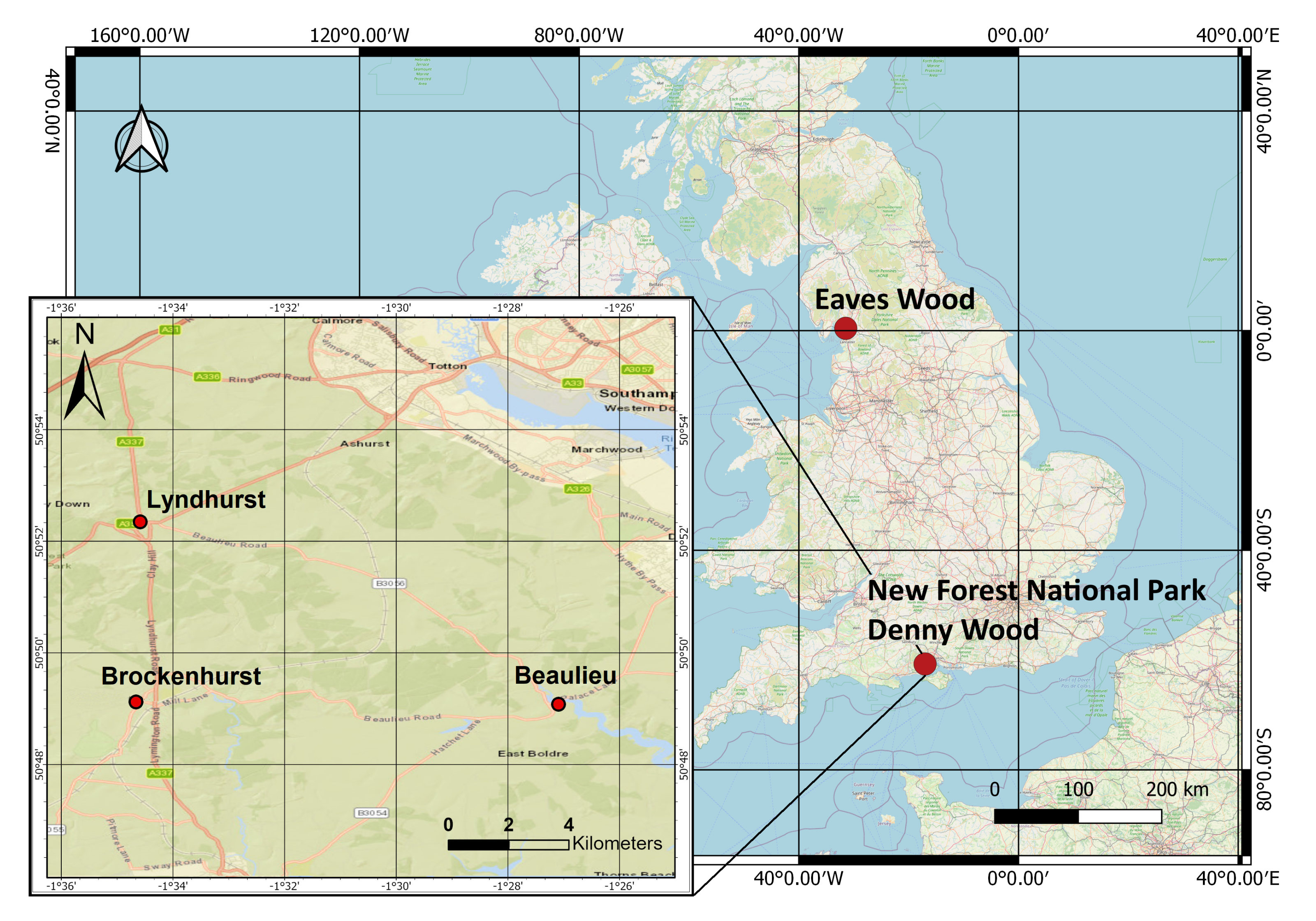
Figure 1 shows the location of the selected flightlines used for testing the performance of the data structures. “Dennys Wood” is part of the “New Forest” National Park, United Kingdom. The two datasets were collected from the same site at different seasons for comparison. The “New Forest” National Park, which is in the southern England, includes actively managed forests. The location of the acquired data lies between three villages; Brockenhurst, Lyndhurst and Beaulieu [29]. The location of those villages is depicted in Figure 1. The national park consists of both deciduous and coniferous forests, which are either seminatural or plantation [30]. Eaves wood is the broadleaved deciduous forest [31] that lies between the Lake District National Park and Lancaster, United Kingdom.

Figure 1.
The study area, within the New Forest National Park, UK, lies between the three villages depicted: Brockenhurst, Lydhurst and Beaulieu.
2.2. Surface Reconstruction
This section is a quick recall of the usage of Marching Cubes algorithm for surface reconstruction, since it is used in this paper to test the performance of the proposed optimisations using the six data structures. For an in-depth description of the algorithms please refer to the associated paper [13]. At first, the waveform samples are voxelised. An algebraic object [32] is defined by a function that represents the voxelised waveform data. That function takes as input a point and returns the value of the voxel that this point lies inside. An isolevel value defines the boundaries of the object to be created. If for a given point, the function is equal to the isolevel then this point lies on the surface of the polygonal model to be reconstructed. Given an isolevel value, the Marching Cubes algorithm [15] can extract a polygonal model from an algebraic object. It first divides the space into cubes. Each cube has eight corners. By using the function of the algebraic object it is derived whether each corner lies inside or outside the surface of the polygonal model. Finally, by using a look up table containing all the possible combinations of corners being inside or outside the polygonal model (to be created), the polygonal surface of the model is reconstructed. Figure 2 shows an example of a polygon generated using the aforementioned methodology. The coloured representation is done by projecting hyperspectral images that were acquired at the same time with the LiDAR data. For more details on how the images were projected and how the polygons could be modified once the various parameters are customised are given at [13].
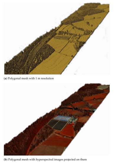
Figure 2.
Example of polygonal models created from the voxelised FW LiDAR using the Marching Cubes algorithm [13].
2.3. Introduction to the Data Structures
This paper compares six approaches for handling and polygonising voxelised full-waveform LiDAR data. The first three approaches use data structures from the literature:
- 1D Array: Influenced by [17], all the data are saved into an 1D array to guarantee coherent memory, even though much memory is consumed in regards to empty voxels.
- Voxel Hashing: “Hash Table” is a data structure that stores the data into an array but in an associative manner. Each data sample has its own associated unique key value. By using a “hash function”, the unique key value is translated into the index of the data sample, and the data sample can be accessed very fast—at constant time —in memory. In the “Voxel Hashing” approach, the intensities of the voxel values are stored inside a hashed table and their unique keys are relevant to the positions of the voxels inside the volume. Similarly to [33], this approach reduces overheads in traversal time of hierarchical structures (process of visiting a node in a tree structure) and on top of that it reduces memory allocation because empty voxels are not stored.
- Octree: This is a hierarchical structure in which each node has up to eight children. Octrees are convenient for representing 3D spaces since the root node represents the entire space (e.g., the voxelised FW LiDAR data), its eight children divide the space equally by eight and so on. In hierarchical structures, traversal time (process of visiting a node in a tree structure) is time consuming. The octree structure though improves memory allocation, since empty voxels are not stored in memory. Additionally, any cuboid voxelised space needs to be fitted into a cube increasing this way the number of empty voxels but since they are not stored into memory they should not be considered as a big issue. In respect to LiDAR interpretation, octrees have been used before for segmentation and classification [34].
The last three approaches are more complicated. A brief summary of them is given here and they are thoroughly explained in Section 2.4, Section 2.5, Section 2.6.
- Integral Volumes: This data structure is an extension of “Integral Images” to 3D. Using Integral Volumes, the sum of any cuboid area is calculated in constant time. By repeatedly dividing the space into cuboids, big empty spaces are quickly identified and ignored during the surface reconstruction [35] (Section 2.4).
- Octree Max and Min: In this approach, the values are saved into an octree, but the surface reconstruction is built-up along with the tree generation. This is slightly different than a traditional octree, because at each branch node its max and min values are saved. This way, areas that are completely full or containing only noise (i.e., no surface crossing those area) are identified at early stages of traversal before reaching the leaves of the trees (Section 2.5).
- Integral Tree: this data structure is proposed at this paper and is a combination of octree and Integral Volumes; the sum of a given branch is given in constant time, but traversal time and backtracking for finding neighbouring voxels remains (Section 2.6).
2.4. Integral Volumes
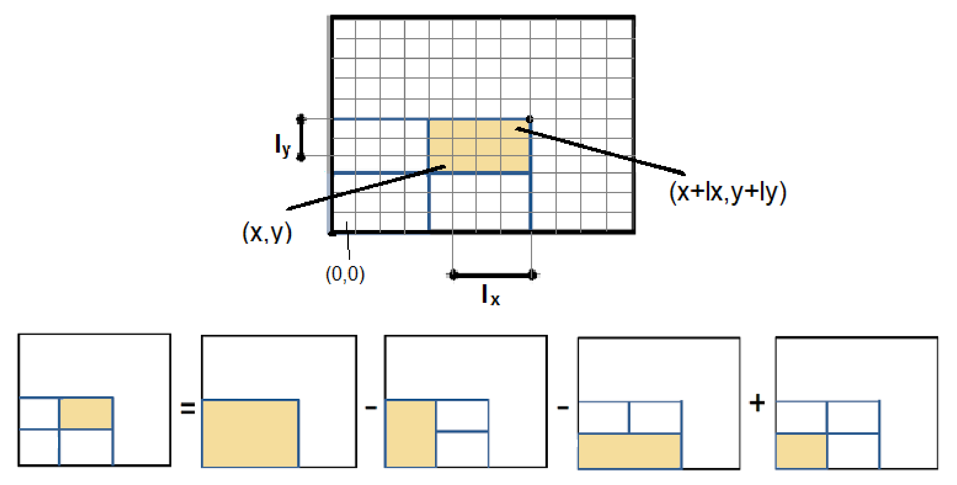
The “Integral Volumes” optimisation is based on the idea of Integral Images, which is an image representation where each pixel value is replaced by the sum of all the pixels that belong to the rectangle defined by the lower left corner of the image and the pixel of interest. An Integral Image is constructed in linear time and the sum of every rectangular area is calculated in constant time, as shown in Figure 3 [36].
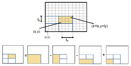
Figure 3.
Once the Integral Image is constructed, the sum of any rectangular area is calculated in constant time.
In this paper, we use the “Integral Volumes” that were briefly tested at [35] and use them to quickly identify and ignore big chunks of empty voxels during polygonisation. The following section explains the mathematics behind “Integral Volumes”, while Section 2.4.2 and Section 2.4.3 give an in depth description about the algorithms invented.
2.4.1. Extending Integral Images to Integral Volumes
As shown in Figure 3, the area of interest is defined by the pixels and and the sum S is given by:
where S is the sum of rectangular area of interest, is the value of the Integral Image at and define the length of the rectangle in the x and y axis respectively.
Extending Integral Images to 3D, the value of the voxel in a 3D Integral Volume becomes equal to the sum of all the values that belong to the box defined by the and included. Therefore, the sum of the box defined by and included is given by:
where is the value of the voxel in the 3D Integral Volume. S is the sum of voxels inside the box, is the value of the voxel in the 3D Integral Volume. and define the length of the box in the x, y and z axis respectively.
2.4.2. Optimisation Algorithm
In “Integral Volumes”, empty areas are quickly identified and ignored during polygonisation using an iterative algorithm. This algorithm continuously splits the volume and checks whether the subvolumes and its neighbouring voxels are empty using the “Integral Volumes”. Please note that all the values below the threshold boundary of the object must be zero and all the nonempty voxels must contain a positive value.
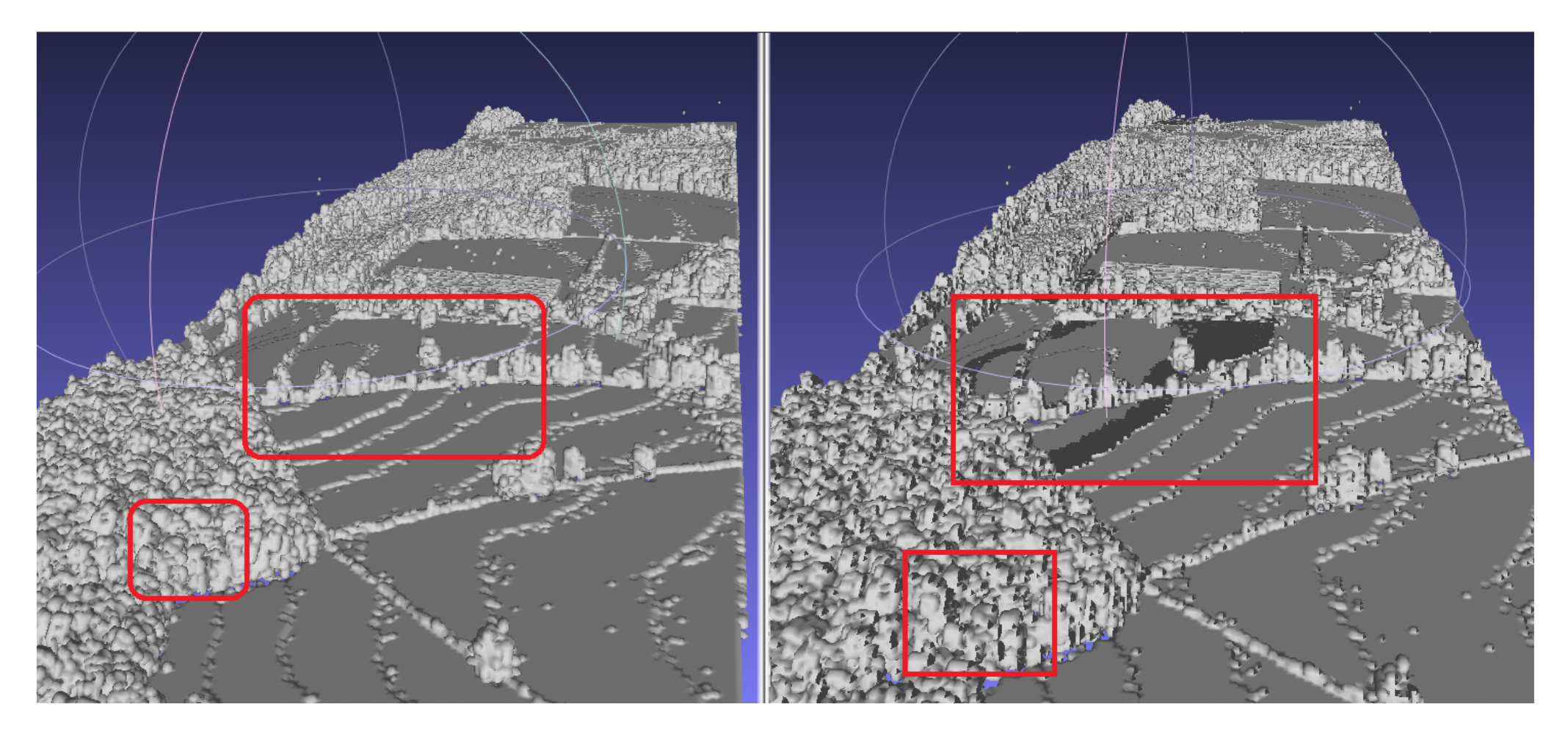
Here it is worth highlighting that, on line 3 of the algorithm it is checked if the neighbouring cubes of a cuboid are empty, because the voxels of the 3D density volume and the cubes in Marching Cubes algorithm are aligned with an offset. If volumes with nonempty neighbouring voxels are ignored, then holes appear on the output polygon mesh (Figure 4).
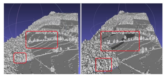
Figure 4.
Comparison between including and ignoring neighbouring voxels; holes appear when ignored. The red boxes show two affected areas. The locations of the red boxes is an approximated association between the two polygons, since the orientation of the polygons slightly varies.
2.4.3. Coding Details for Faster Implementation
Implementation details contribute to the efficiency and speed up of the algorithm. Significant improvements are achieved by reducing recursions, big memory allocations and if statements, since memory jumps are time expensive. As shown in Algorithm 1, a while loop is used to avoid recursion.
| Algorithm 1 Integral Volumes Optimisation Algorithm [35] |
|
Regarding memory consumption, a stack was chosen over a queue to decrease the amount of cubes saved into the data structure simultaneously. A queue is a first in first out data structure, while a stack accesses data in a last in first out order. In every iteration, it is ideal to interpret the smallest saved cube, such that the possibility of being polygonised is higher and the possibility of storing another cube is less. A queue guarantees cubes with approximately the same size, since the big cubes will be added first and sequentially divided first. In contrast, a stack guarantees the smallest possible number of cubes saved. The larger cubes are stored in the bottom of the stack while the smaller ones are interpreted first because they are always the last one divided and inserted into the stack. For that reason, a stack guarantees the lowest memory usage.
In Algorithm 1, an issue exists: how to quickly identify the side to be divided next? Ideally, the usage of if-statements should be low because they contain many time expensive memory jumps. For that reason, bitwise operations were embedded to reduce their usage. A cube is defined with its position, its size, the next side to be divided s and its divisible sides D. The parameter s takes the values 1, 2, 3 for the x, y, z sides respectively. The parameter D is an integer consisting of the sum of three numbers or or or indicating whether the sides x, y, z are divisible or not (Table 1). The parameter D takes the value between and covering all the possible cases of divisible sides as shown in Table 2 and Table 3. For example if x and z are the divisible sides, then . The bitwise operations and the faster implementations of the Integral Volumes optimisations are demonstrated in Algorithm 2.
| Algorithm 2 Integral Volumes Optimisation Algorithm |
|

Table 1.
Values of divisible sides.

Table 2.
How to calculate the value of D, which represents the divisible sides of a cuboid.

Table 3.
How to calculate the value of divisible sides (D) in binary representation.
2.5. Octree Max and Min
“Integral Volumes” quickly identifies and ignores empty spaces during polygonisation, but it allocates memory for the entire volume. For that reason, the “Octree Max and Min” data structure has been investigated.
The “Octree Max and Min” data structure avoids storing empty voxels and also identifies empty areas during polygonisation. The polygonisation is built on the traversal of the octree, as explained in Algorithm 3. Similar to “Integral Volumes”, a stack is used to avoid recursion and reduce memory jumps. As in “Integral Volumes”, it is essential to check neighbouring voxels when a branch of the “Octree Max and Min” data structure could be ignored. However, because the branches of the octree are always cubic, it is not trivial to check whether they are empty or not. For that reason, if a branch is empty then we loop through its edges and polygonise them according to look up table of the the Marching Cubes algorithm.
| Algorithm 3 Embedding Marching Cubes into an octree |
|
Embedding the polygonisation of volumetric data into an octree has been done before [37]. Nevertheless, here, the max and min values of each branch are stored into the corresponding node to speed up polygonisation. This enables checking whether the leaves of a branch lie either only inside or only outside the implicit object. If they do, then no surface is crossing that branch and it can be discarded (after polygonising its edges).
2.6. Integral Tree
2.6.1. Main Idea
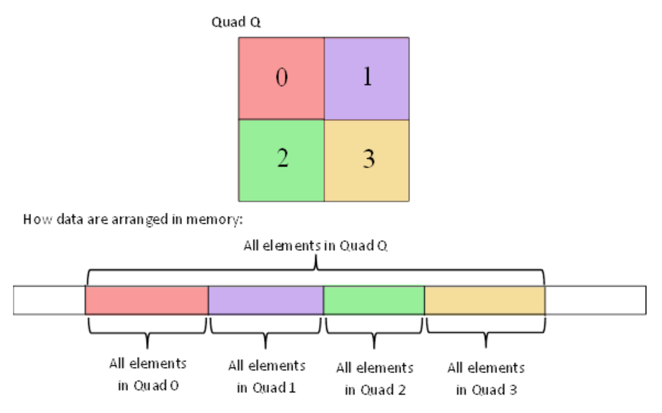
The “Integral Tree” is a new data structure that attempts to preserve some properties of the “Integral Images” embedded in a tree structure. Every “Integral Tree” consists of two elements: an integral 1D-array and a tree. During construction, at first all the values from the tree node are stored inside an 1D-array, such that the following condition applies: all the values of every branch are adjacent inside the 1D-array. Once the values are stored and sorted, the 1-D array is converted to integral. Additionally, the root node of each branch contains two parameters . The number k is the number of nodes, which contain values, of the branch (e.g., for an octree, it is all its leaf nodes) and the pointer points to its first stored node value within the integral 1D-array (Figure 5).

Figure 5.
Ordering of tree elements.
The aforementioned rules can be applied to any tree structures including binary trees, quadtrees and octrees. To better perceive how this data structure works, let us assume that there is a quadtree representing grid values. Figure 6 depicts how the grid should be recursively subdivided and how the corresponding node values can be stored into the 1D-array in order to fulfil the adjacency condition of the “Integral Tree”. In addition, Section 2.6.2 gives an example of an “Integral Binary Tree”.

Figure 6.
Illustration of how to save the values of an “Integral Quad Tree” into the 1D-array, in order to preserve the condition of “Integral Trees”.
2.6.2. Integral Binary Tree Example
An example of applying the idea of “Integral Tree” into a binary tree is given for clarification (Figure 7).
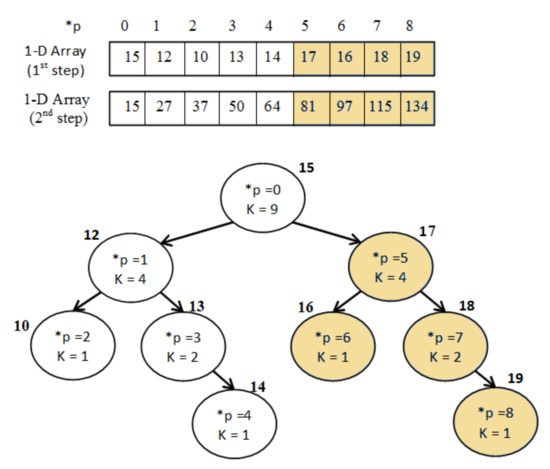
Figure 7.
Example of “Integral Binary Tree”.
Firstly, the values of the binary tree are sorted into the 1D-array A as in order to fulfil the adjacency condition. Secondly, the array A is modified as in order to become integral using the following equation:
Then the sum S of a branch, with (, k) parameters, is calculated at constant time as follows:
For instance, the sum of the blue branch on Figure 7 is , which is correct since .
2.6.3. Integral Octree for Surface Reconstruction
For an “Integral Octree”, all the values saved into the integral 1D-array are the values of the leaf nodes since the rest are connecting nodes. For the surface reconstruction, an “Integral Octree” is implemented and the same polygonisation algorithm as “Octree Max and Min” are used (Algorithm 3). The only difference is the comparison at Line 6 of Algorithm 3; instead of checking the max and min values, the sum of the branch is checked instead. If the sum is smaller than the isolevel value then no surface is crossing that area and the branch is discarded.
3. Results
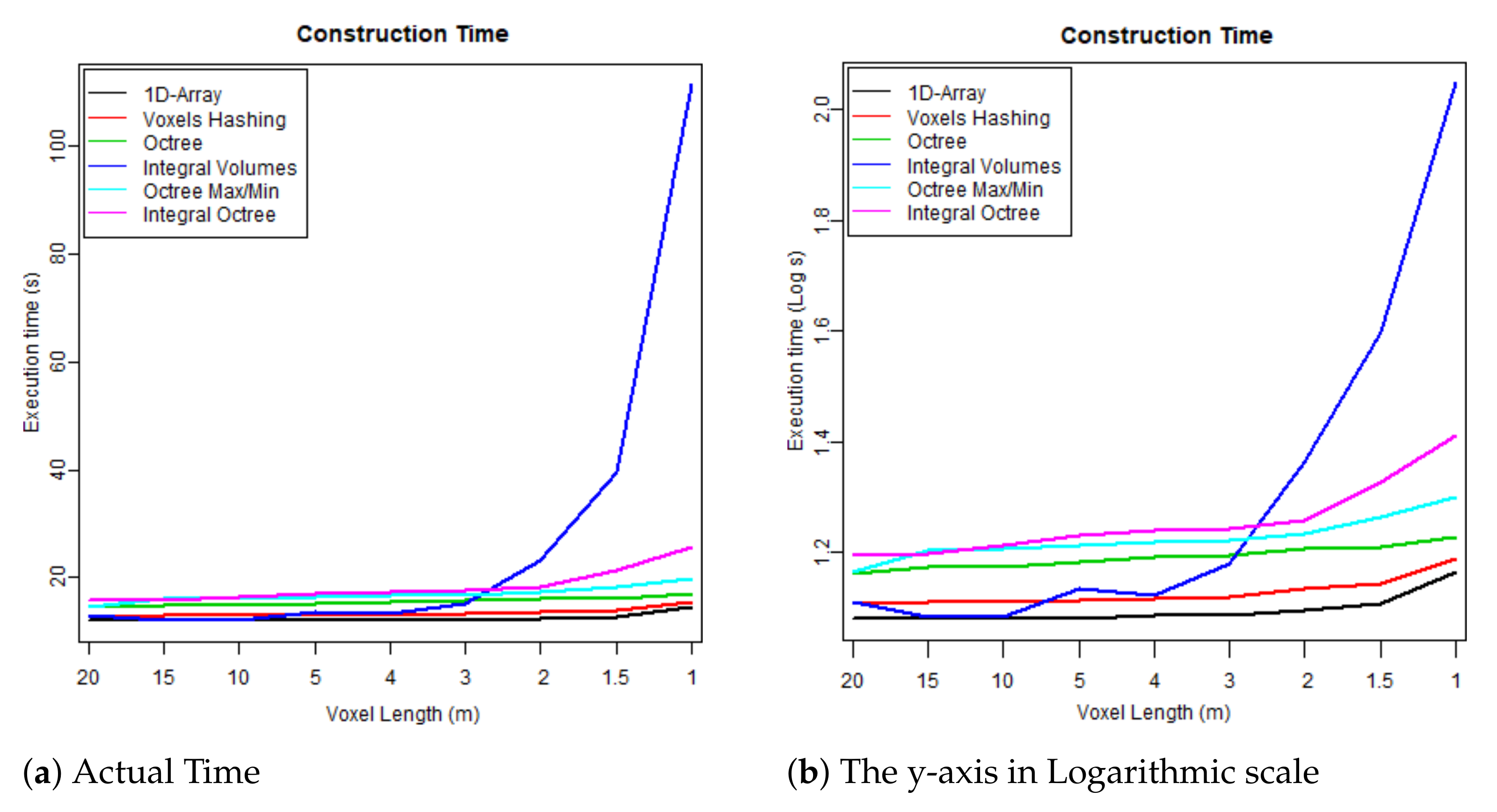
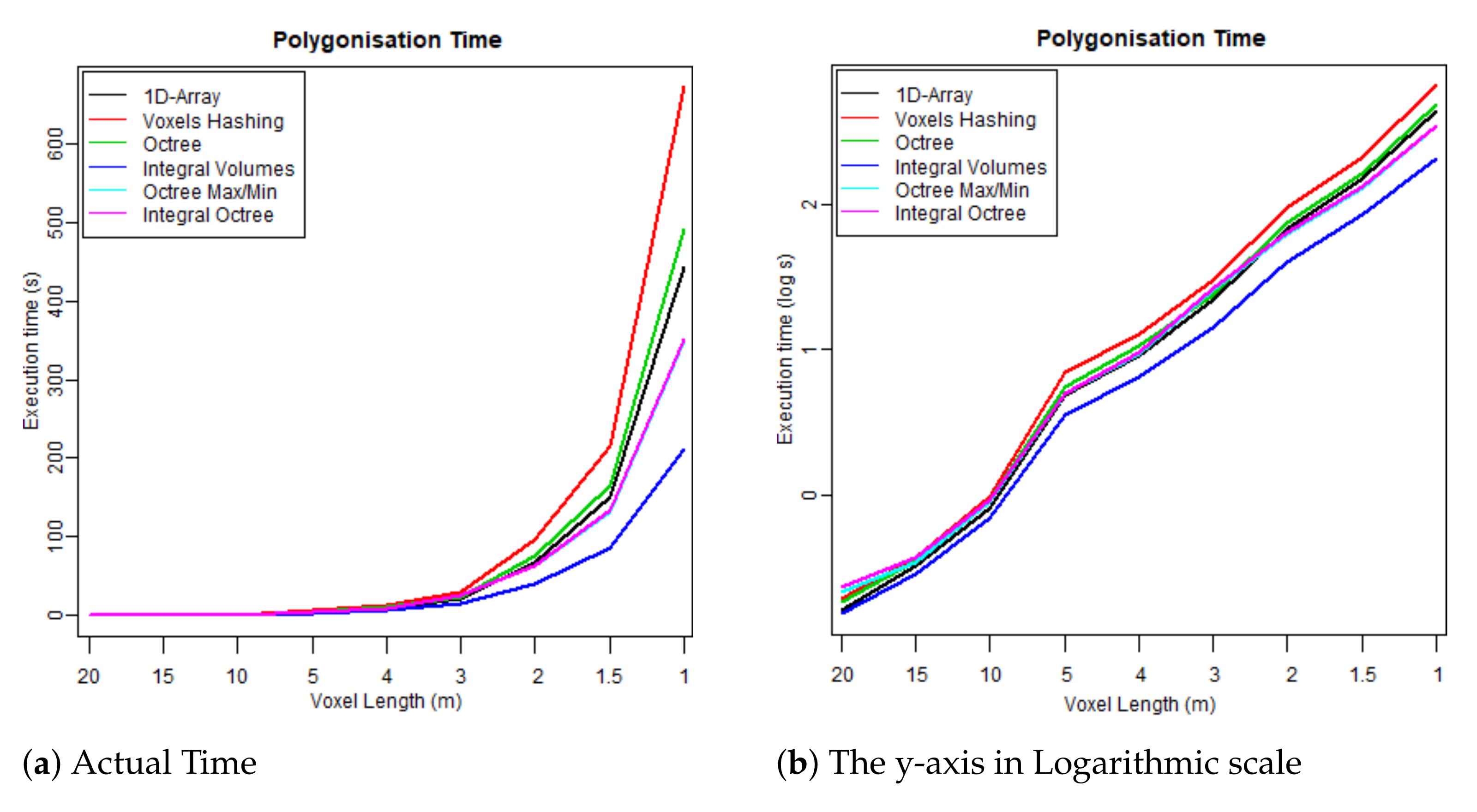
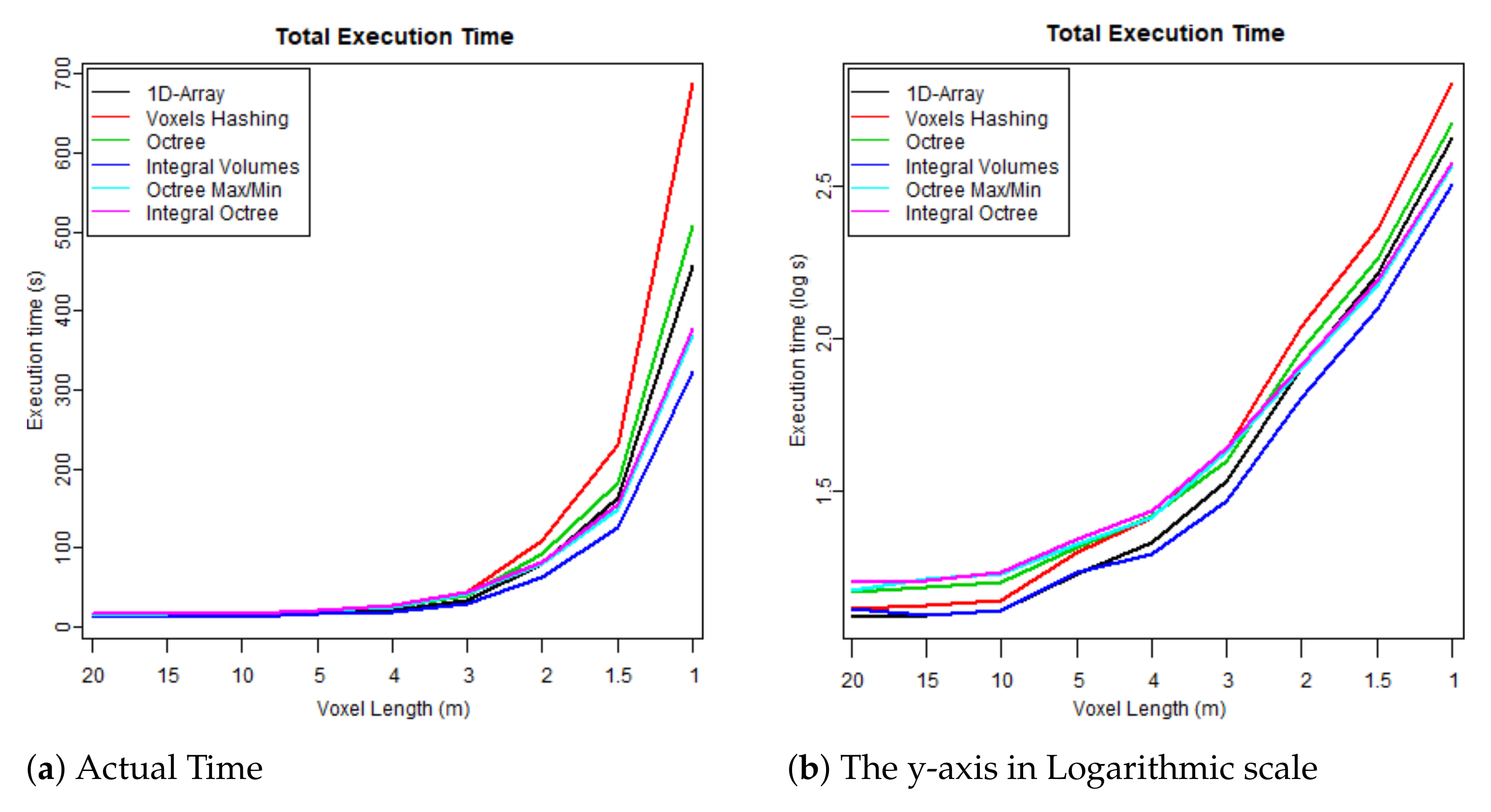
The implemented algorithms are beneficial in different aspects: speeding up execution and/or decreasing memory usage. To better understand the performance of the algorithms, the voxel length (m), the number of voxels in the x,y,z axes and the percentage of empty voxels are taken into consideration. The smaller the voxel length is, the more voxels exist because when the voxel length decreases the resolution of the voxelised FW LiDAR data increases. Additionally, for every test, the total execution time and maximum memory consumption are measured. Execution time is further divided into construction time, which is the time required to read the LAS file and construct the data structure, and polygonisation. The performance has been tested in two groups of test cases:
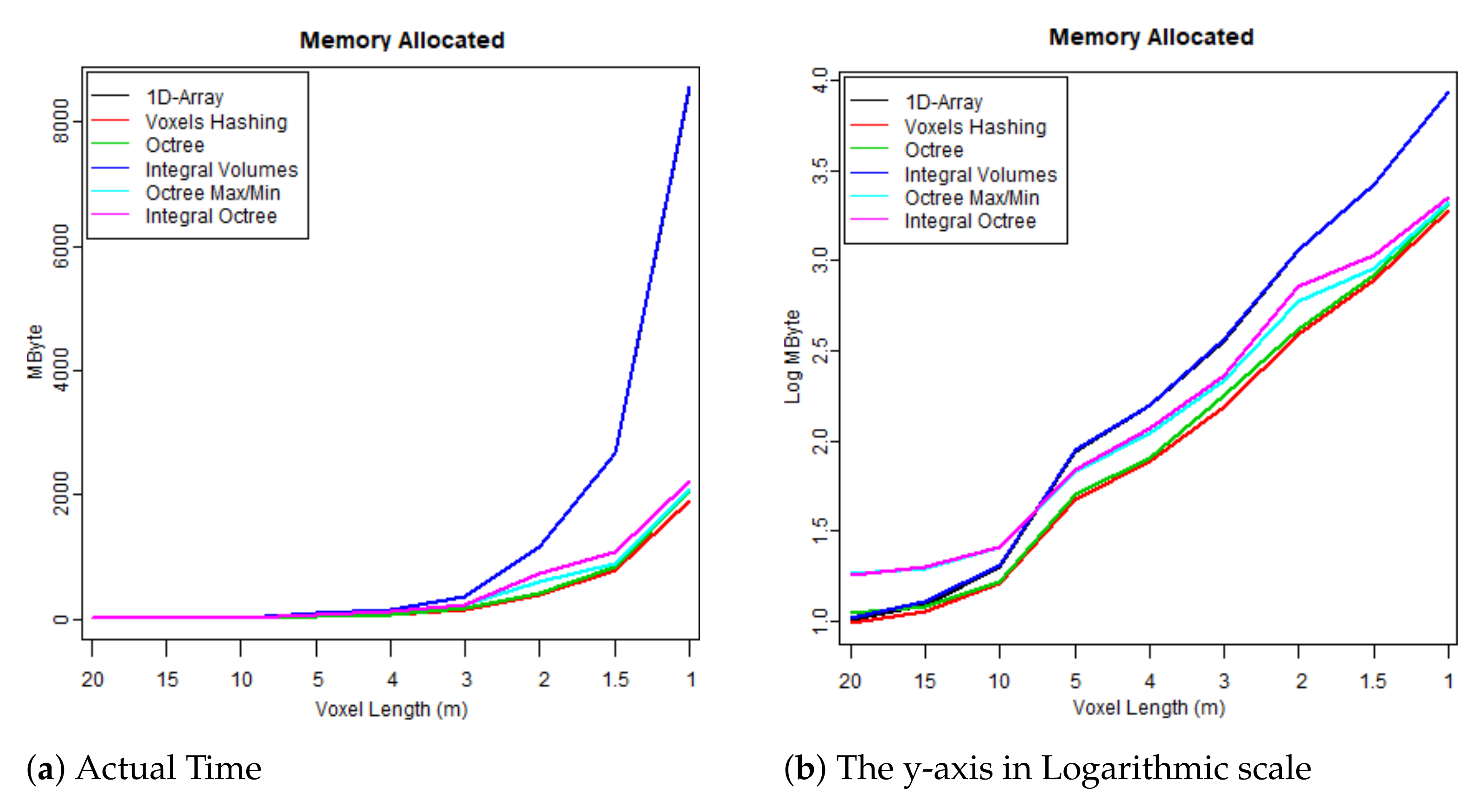
- The first test case uses one flightline (the “LDR-FW-FW10_01-201009821.LAS” from New Forest) and focuses on its performance while changing resolution of the voxelised FW LiDAR data (voxel length in meters). The results of the first group are given in Table 4 and visualised in the graphs depicted in Figure 8, Figure 9, Figure 10 and Figure 11. As shown in Figure 8, “1D-Array” and “Integral Volumes” consume the highest memory, which is approximately the same (Table 4).
 Table 4. Results: Execution time and memory consumption, Con = Construction, Pol = Polygonisation, MByte = Max Memory, Len = Voxel Length that relates to the resolution of the volume.
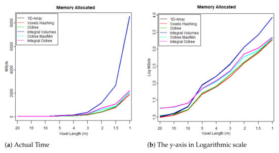 Figure 8. Maximum memory consumption at run time.
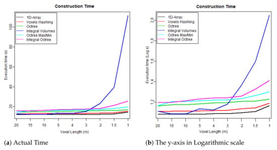 Figure 9. Time required to build each data structure by voxelising the FW LiDAR samples (Table 4).
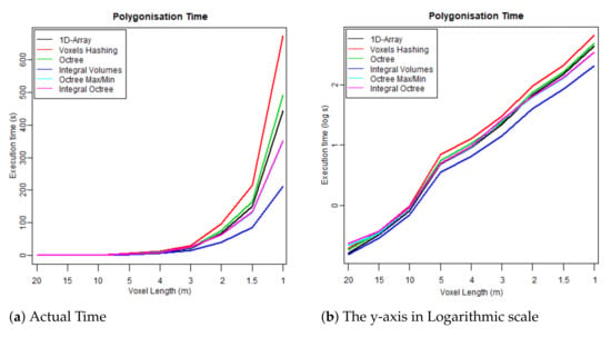 Figure 10. Time required to reconstruct the surface from the voxelised FW LiDAR data (Table 4).
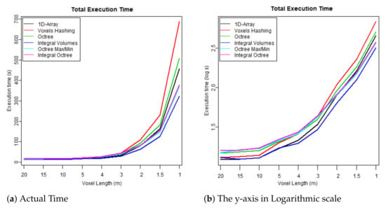 Figure 11. Total executable time including both construction and polygonisation (Table 4).
 - The second test checks whether there are significant performance differences when the algorithms are applied on different flightlines and study areas. It, therefore, tests the performance of the data structure on three flightlines: (1) from the “New Forest” forest dataset (LDR-FW-FW10_01-201009822.LAS), (2) from the “Dennys Wood” dataset (LDR-FW10_01-201018713.LAS) and (3) from the “Eaves Wood” (LDR-FW-GB12_04-2014-083-13.LAS). The results of the second group of test cases are given in Table 5. More information about the datasets and the study areas are given in Section 2.1.
 Table 5. Execution time and memory consumption results from three different flightlines.
4. Discussion
To briefly sum up, the following six data structures have been implemented and their performance has been tested for reconstructing 3D polygonal models from voxelised FW LiDAR data:
- 1D-Array: Simple array that keeps data coherent in memory for quick access.
- Voxel Hashing: A hashed table is used for storing the intensity values of the voxels [33].
- Octree: Simple hierarchical structure, but it is scanline implementation (i.e., it cannot identify and ignore big chunks of empty voxels).
- Integral Volumes: Extension of “Integral Images” that allows finding the sum of any cuboid area in constant time. It is used for quickly identifying and ignoring empty areas during polygonisation.
- Octree Max/Min: The polygonisation is embedded into an hierarchical data structure [37]. The max and min values of each branch are stored to identify and ignore branches that either only contain low level noise or are completely inside the algebraic object.
- Integral Octree: new data structure proposed at this paper and an attempt to preserve properties from both “Octree Max/Min” and “Integral Volumes”.
Each one of the aforementioned data structures has different properties. The first three implementations are scanline algorithms, which means that polygonisation is linear and all the voxels, including the empty ones, are checked for generating triangles primitives. Some data structures are taken from the literature to test how well they perform on this specific datasets while others are new and presented into this paper. Table 6 summarises their properties and the problems each data structure attempts to resolve.

Table 6.
Summarising the addressed challenges and the properties of all the data structures implemented.
Before proceeding to the comparison of the data structures, it is worth mentioning a limitation. Even though noisy points are classified during preprocessing by NERC-ARF-DAN, the tools we implement use the limits stored inside the LAS files for defining the size of the voxelised space [11]. This implies that the noisy points are ignored during voxelisation but the voxelised space is not resized. Therefore, hierarchical structures—that do not store empty voxels—has been benefited from the removal of the noisy waveforms, but structures that require to store the values of all the voxels are not. This may be resolved by reading the LAS files twice: once for defining the size of the voxelised space and once for the voxelisation process. This will increase construction time and it should, therefore, be considered according to the type of the structure to be used and the size of the data to be loaded.
Overall, “Integral Volumes” is the fastest one but it consumes as much memory as the original “1D-Array”. Its performance is better than the “Octree Max and Min” because:
- Elements are accessed in constant time while traversing a tree requires at least time, when the tree is balanced, and up to for unbalanced trees.
- The size of the volume is the original cuboid while any octree data structure requires a cubic space that is a power of two. This results into extending the boundaries of the 3D voxelised FW LiDAR data, including big empty areas and building deeper and unbalanced trees (increased traversal time).
- Neighbour-finding is faster than octrees since no backtracking is required.
- Checking whether a surface is crossing the edges of an empty area is much faster using the “Integral Volumes” because the sum of any volume is calculated in constant time. Therefore, checking whether the neighbours of an empty cell are also empty is trivial. In contrast, the “Octree Max/Min” and “Integral Tree” data structures must loop through all the voxels at the edges of an empty branch to avoid generating holes.
Regarding the “Voxel Hashing”, faster results were expected than the “Octree” because it does not require traversal for reaching elements, but it is very likely to have more memory jumps, considering that the implementation of the octree structures keeps the children of every branch coherent in memory for faster interpretation. Additionally, during the expansion of hashed tables, many reallocation occurs.
Furthermore, “Octree Max and Min” and the “Integral Octree” have similar results. In the tests, the isolevel was set lower than the noise threshold and for that reason the empty branches were the ones discarded at the tests (Line 6 of Algorithm 3). If the isolevel was lower than the noise threshold, then the low level noise would have affected the “Octree Max and Min” less than the “Integral Octree”; the “Octree Max and Min” check whether the max value is below the threshold, while the “Integral Octree” the sum of the leaves. Additionally, “Integral Octree” consumes more memory for saving the leaves into an 1D-array, but even though “Integral Octree” generally performed worse than the “Octree Max/Min” in the tests of Table 4 and Table 5, it should be beneficial in multiresolution direct volumetric rendering and blurring the volume for noise removal.
It further worth mentioning that even though this specific paper tested the performance of the data structures using FW LiDAR data, this research has a bigger application domain. Firstly, the data structures can be used for interpreting a variety of voxel-based datasets. Secondly, iso-surface extraction is a big field in Computer Graphics used in Medical imaging [38] and Animation Production [39]. Therefore, this research is not restricted to the usage of LiDAR data but has multiple applications.
5. Conclusions
Advances in Remote Sensing, Medical Imagery and Animation production raises the need for efficient data management. In respect to airborne LiDAR technologies, the full-waveform (FW) airborne LiDAR data are 5 to 10 times larger than discrete LiDAR data. Most existing workflows only support handling of discrete LiDAR or peak points extracted from FW LiDAR, since the increased amount of information recorded makes handling difficult. This paper investigated the performance of six data structures for managing voxelised FW LiDAR data during 3D polygonal model creation. The six data structures are (1) 1D-Array, (2) Voxel Hashing, (3) Octree, (4) Integral Volumes, (5) Octree Max/Min, (6) Integral Octree. The “Integral Octree” is proposed in this paper and it is an attempt to preserve the properties of “Integral Volumes” in an hierarchical structure. According to the results, “Integral Volumes”, which are able to return the sum of any cuboid area at constant time, is the fastest data structure for the 3D polygonal model creation of voxelised FW LiDAR data, but it consumes the most memory, equal to the “1D-Array” data structure. It is, therefore, concluded that each data structure has different properties and both memory consumption and time efficiency need to be taken into consideration, as well as the type of the interpretation to be performed. Finally, even though this paper investigates the performance of these data structures for interpreting voxelised FW LiDAR data, the application domain is much bigger since it could be utilised in any type of volumetric data.
Author Contributions
Conceptualisation, M.M., N.D.F.C., D.C. and M.G.G.; methodology, M.M.; software, M.M.; validation, M.M.; formal analysis, M.M.; investigation, M.M.; resources, M.M., N.D.F.C. and M.G.G.; data curation, M.M.; writing—original draft preparation, M.M.; writing—review and editing, M.M., N.D.F.C., D.C. and M.G.G.; visualization, M.M.; supervision, N.D.F.C. and M.G.G.; project administration, N.D.F.C. and M.G.G.; funding acquisition, N.D.F.C., D.C. and M.G.G. All authors have read and agreed to the published version of the manuscript.
Funding
This research was funded by the Centre for Digital Entertainment (CDE) with Grant reference number “EP/L016540/1” and Plymouth Marine Laboratory. The APC was funded by the UKRI Block Grant fund of University of Bath, UK. Data from the NERC ARF are provided courtesy of NERC via the Centre for Environmental Data Analysis (CEDA) and were processed by NEODAAS.
Institutional Review Board Statement
Not applicable.
Informed Consent Statement
Not applicable.
Data Availability Statement
Not applicable.
Acknowledgments
The data were provided by the NERC Airborne Research and Facility (ARF).
Conflicts of Interest
The authors declare no conflict of interest.
Abbreviations
The following abbreviations are used in this manuscript:
| 1D | 1 dimensional |
| 2D | 2 dimensional |
| 3D | 3 dimensional |
| ARF | Airborne Research Facility |
| CDE | Centre for Digital Entertainment |
| FW | Full Waveform |
| GPU | Graphics Processing Unit |
| LiDAR | Light Detection and Ranging |
| MDPI | Multidisciplinary Digital Publishing Institute |
| MRI | Magnetic Resonance Imaging |
| NERC | Natural Environment Research Council |
| SIMD | Single Instruction, Multiple Data |
References
- Wanger, W.; Ullrich, A.; Melzer, T.; Briese, C.; Kraus, K. From single-pulse to full-waveform airborne laser scanners. ISPRS J. Photogramm. Remote. Sens. 2004, 60, 100–112. [Google Scholar]
- LAS Specification. VERSION 1.3—R11; The American Society for Photogrammetry and Remote Sensing: Bethasda, MD, USA, 2010. [Google Scholar]
- Riegl. Long-Range Airborne Laser Scanner for Full Waveform Analysis (LMS-Q680i); RIEGL Laser Measurement Systems GmbH: Horn, Austria, 2012. [Google Scholar]
- Miltiadou, M.; Agapiou, A.; Gonzalez Aracil, S.; Hadjimitsis, D.G. Detecting Dead Standing Eucalypt Trees from Voxelised Full-Waveform Lidar Using Multi-Scale 3D-Windows for Tackling Height and Size Variations. Forests 2020, 11, 161. [Google Scholar] [CrossRef]
- Zhou, T.; Popescu, S.; Malambo, L.; Zhao, K.; Krause, K. From LiDAR waveforms to Hyper Point Clouds: A novel data product to characterize vegetation structure. Remote Sens. 2018, 10, 1949. [Google Scholar] [CrossRef]
- Miltiadou, M.; Campbell, N.D.; Aracil, S.G.; Brown, T.; Grant, M.G. Detection of dead standing Eucalyptus camaldulensis without tree delineation for managing biodiversity in native Australian forest. Int. J. Appl. Earth Obs. Geoinf. 2018, 67, 135–147. [Google Scholar] [CrossRef]
- Wanger, W.; Ullrich, A.; Ducic, V.; Maizer, T.; Studnicka, N. Gaussian decompositions and calibration of a novel small-footprint full-waveform digitising airborne laser scanner. ISPRS J. Photogramm. Remote. Sens. 2006, 60, 100–112. [Google Scholar] [CrossRef]
- Bunting, P.; Armston, J.; Clewley, D.; Lucas, R.M. Sorted pulse data (SPD) library—Part II: A processing framework for LiDAR data from pulsed laser systems in terrestrial environments. Comput. Geosci. 2013, 56, 207–215. [Google Scholar] [CrossRef]
- Chauve, A.; Bretar, F.; Durrieu, S.; Pierrot-Deseilligny, M.; Puech, W. FullAnalyze: A research tool for handling, processing and analysing full-waveform LiDAR data. In Proceedings of the IEEE International Geoscience and Remote Sensing Symposium, Cape Town, South Africa, 12–17 July 2009. [Google Scholar] [CrossRef]
- Isenburg, M. PulseWaves: An Open, Vendor-Neutral, Stand-Alone, LAS-Compatible Full Waveform LiDAR Standard; rapidlasso GmbH: Gilching, Germany, 2012. [Google Scholar]
- Miltiadou, M.; Michael, G.; Campbell, N.D.; Warren, M.; Clewley, D.; Hadjimitsis, D.G. Open source software DASOS: Efficient accumulation, analysis, and visualisation of full-waveform lidar. In Proceedings of the Seventh International Conference on Remote Sensing and Geoinformation of the Environment (RSCy2019), Paphos, Cyprus, 18–21 March 2019; Volume 11174, p. 111741. [Google Scholar] [CrossRef]
- Persson, A.; Soderman, U.; Topel, J.; Ahlberg, S. Visualisation and Analysis of full-waveform airborne laser scanner data. Int. Arch. Photogramm. Remote. Sens. Spat. Inf. Sci. 2005, 36, 103–108. [Google Scholar] [CrossRef]
- Miltiadou, M.; Warren, M.; Grant, M.; Brown, M. Alignment of hyperspectral imagery and full-waveform LiDAR data for visualisation and classification purposes. Int. Arch. Photogramm. Remote. Sens. Spat. Inf. Sci. ISPRS Arch. 2015, 40, 1257. [Google Scholar] [CrossRef]
- Hanrahan, P. Ray tracing algebraic surfaces. ACM SIGGRAPH Comput. Graph. 1983, 17. [Google Scholar] [CrossRef]
- Lorensen, W.E.; Cline, H.E. Marching cubes: A high resolution 3D surface construction algorithm. ACM Siggraph Comput. Graph. 1987, 21, 163–169. [Google Scholar] [CrossRef]
- Levoy, M. Display of surfaces from volume data. IEEE Comput. Graph. Appl. 1988, 8, 29–37. [Google Scholar] [CrossRef]
- Hadwiger, M.; Beyer, J.; Jeong, W.K.; Pfister, H. Interactive Volume Exploration of Patascale Microscopy Data Streams Using Visualizatin-Driven Virtual Memory Approach. IEEE Trans. Vis. Comput. Graph. 2012. [Google Scholar] [CrossRef] [PubMed]
- Crassin, C.; Neyret, F.; Lefebvre, S.; Eisemann, E. GigaVoxels: Ray-Guided Streaming for Efficient and Detailed Voxel Rendering. In Proceedings of the 2009 Symosium on Interactive 3D Graphics and Games, Boston, MA, USA, 27 February–1 March 2009; pp. 15–22. [Google Scholar] [CrossRef]
- Laine, S.; Karras, T. Efficient Sparse Voxel Octrees. IEEE Trans. Vis. Comput. Graph. 2011, 17, 1048–1059. [Google Scholar] [CrossRef]
- Rodrigues de Araujo, B.; Pires Jorge, J.A. Adaptive polygonization of implicit surfaces. Sci. Direct Comput. Graph. 2005, 29, 686–696. [Google Scholar] [CrossRef]
- Hartmann, E. A marching method for the triangulation of surfaces. Vis. Comput. 1998, 14, 95–108. [Google Scholar] [CrossRef]
- Hansen, C.D.; Hinker, P. Massively Parallel Isosurface Extraction. In Proceedings of the 3rd Conference on Visualization ’92, Boston, MA, USA, 19–23 October 1992; pp. 77–83. [Google Scholar] [CrossRef]
- Galbraith, C.; MacMurchy, P.; Wyvill, B. BlobTree Trees. IEEE Comput. Graph. Int. 2004, 78–85. [Google Scholar] [CrossRef]
- Sutter, H.; Alexandrescu, A. C++ Coding Standards: 101 Rules, Guidlines, and Best Practices; Addison-Wesley: Boston, MA, USA, 2004. [Google Scholar]
- Trochta, J.; Krucek, M.; Vrska, T.; Kral, K. 3D Forest: An application for descriptions of three-dimensional forest structures using terrestrial LiDAR. PLoS ONE 2017, 12, e0176871. [Google Scholar] [CrossRef]
- Babahajiani, P.; Fan, L.; Kämäräinen, J.K.; Gabbouj, M. Urban 3D segmentation and modelling from street view images and LiDAR point clouds. Mach. Vis. Appl. 2017, 28, 679–694. [Google Scholar] [CrossRef]
- Wang, R.; Peethambaran, J.; Chen, D. LiDAR point clouds to 3-D Urban Models: A review. IEEE J. Sel. Top. Appl. Earth Obs. Remote. Sens. 2018, 11, 606–627. [Google Scholar] [CrossRef]
- Isenburg, M. LAStools—Efficient Tools for LiDAR Processing. 2012. Available online: http:http://www.cs.unc.edu/~{}isenburg/lastools/ (accessed on 9 October 2012).
- Sumnall, M.J.; Hill, R.A.; Hinsley, S.A. Comparison of small-footprint discrete return and full waveform airborne lidar data for estimating multiple forest variables. Remote Sens. Environ. 2016, 173, 214–223. [Google Scholar] [CrossRef]
- Newton, A.; Cantarello, E.; Myers, G.; Douglas, S.J.; Tejedor, N. The Condition and Dynamics of New Forest Woodlands; Pisces Publications: Bournemouth, UK, 2010. [Google Scholar]
- Abd Latif, Z.; Blackburn, G.A. Extraction of gap and canopy properties using LiDAR and multispectral data for forest microclimate modelling. In Proceedings of the IEEE 2010 6th International Colloquium on Signal Processing & Its Applications, Mallaca City, Malaysia, 21–23 May 2010; pp. 1–5. [Google Scholar] [CrossRef]
- Blinn, J.F. A Generalization of Algebraic Surface Drawing. ACM Trans. Graph. TOG 1982, 1, 235–256. [Google Scholar] [CrossRef]
- Nießner, M.; Zollhöfer, M.; Izadi, S.; Stamminger, M. Real-time 3d reconstruction at scale using voxel hashing. ACM Trans. Graph. TOG 2013, 32, 169. [Google Scholar] [CrossRef]
- Wang, M.; Tseng, Y.H. Lidar data segmentation and classification based on octree structure. Parameters 2004, 1, 5. [Google Scholar]
- Miltiadou, M.; Campbell, N.D.; Brown, M.; Cosker, D.; Grant, M.G. Improving and optimising visualisations of full-waveform LiDAR data. ACM Digit. Libr. 2016, 45–47. [Google Scholar] [CrossRef]
- Crow, F.C. Summed-Area Tables for Texture Mapping. ACM Comput. Graph. 1984, 18, 207–212. [Google Scholar] [CrossRef]
- Wilhelms, J.; Van Gelder, A. Octrees for faster isosurface generation. ACM SIGGRAPH Comput. Graph. 1990, 24, 57–62. [Google Scholar] [CrossRef]
- Lee, T.Y.; Lin, C.H. Growing-cube isosurface extraction algorithm for medical volume data. Comput. Med Imaging Graph. 2001, 25, 405–415. [Google Scholar] [CrossRef]
- Zhao, Y.; Wei, X.; Fan, Z.; Kaufman, A.; Qin, H. Voxels on fire [computer animation]. In Proceedings of the IEEE Visualization, Seattle, WA, USA, 19–24 October 2003; pp. 271–278. [Google Scholar] [CrossRef]
Publisher’s Note: MDPI stays neutral with regard to jurisdictional claims in published maps and institutional affiliations. |
© 2021 by the authors. Licensee MDPI, Basel, Switzerland. This article is an open access article distributed under the terms and conditions of the Creative Commons Attribution (CC BY) license (http://creativecommons.org/licenses/by/4.0/).

