Abstract
Mobile laser scanning (MLS) systems are often used to efficiently acquire reference data covering a large-scale scene. The terrestrial laser scanner (TLS) can easily collect high point density data of local scene. Localization of static TLS scans in mobile mapping point clouds can afford detailed geographic information for many specific tasks especially in autonomous driving and robotics. However, large-scale MLS reference data often have a huge amount of data and many similar scene data; significant differences may exist between MLS and TLS data. To overcome these challenges, this paper presents a novel deep neural network-based localization method in urban environment, divided by place recognition and pose refinement. Firstly, simple, reliable primitives, cylinder-like features were extracted to describe the global features of a local urban scene. Then, a probabilistic framework is applied to estimate a similarity between TLS and MLS data, under a stable decision-making strategy. Based on the results of a place recognition, we design a patch-based convolution neural network (CNN) (point-based CNN is used as kernel) for pose refinement. The input data unit is the batch consisting of several patches. One patch goes through three main blocks: feature extraction block (FEB), the patch correspondence search block and the pose estimation block. Finally, a global refinement was proposed to tune the predicted transformation parameters to realize localization. The research aim is to find the most similar scene of MLS reference data compared with the local TLS scan, and accurately estimate the transformation matrix between them. To evaluate the performance, comprehensive experiments were carried out. The experiments demonstrate that the proposed method has good performance in terms of efficiency, i.e., the runtime of processing a million points is 5 s, robustness, i.e., the success rate of place recognition is 100% in the experiments, accuracy, i.e., the mean rotation and translation error is (0.24 deg, 0.88 m) and (0.03 deg, 0.06 m) on TU Delft campus and Shanghai urban datasets, respectively, and outperformed some commonly used methods (e.g., iterative closest point (ICP), coherent point drift (CPD), random sample consensus (RANSAC)-based method).
1. Introduction
Localization techniques help people understand their surrounding environment by getting information about their position in a geographic reference map [1]. Global Navigation Satellite System (GNSS) is a widely used localization technique. Unfortunately, a high accuracy of GNSS localization requires a scenario where there is less signal transmission interruption. Urban environment is complicated, involving trees, buildings and other tall objects can easily obstruct the GNSS signals. In contrast, localization based on 3D point cloud is signal transmission free. Point clouds acquired from laser scanning systems (e.g., mobile laser scanning-MLS and airborne laser scanning-ALS) at a large-scale provide a reliable reference map over time. In addition, a terrestrial laser scanner (TLS) is used to capture the surfaces with high detailed, dense, accurate data points at the small-scale scene. Accurately and efficiently integrating TLS data to the ALS or MLS reference data can offer highly detailed geographic information, which can subsequently be used in various applications, for example, autonomous driving and robotics navigation [2,3].
3D point cloud localization is a process to determine a rigid transformation with 6 degrees of freedom (DOF) (i.e., three rotational movements around x, y, and z axes, and three translational movements along those axes), which is also known as integration, registration, alignment or fusion in related literature. The MLS system is often equipped with a positioning and orientation system that provides an efficient way to capture large-scale geo-referenced point clouds [4]. Modern TLS devices have accurate level compensator that reduces the relative rotation between scans to the azimuth [5]. Therefore, the search space has only 4DOF (i.e., one rotational movement around the z axis, and three translational movements along those axes) when mapping TLS to MLS data. However, some challenges for TLS to MLS localization are: (1) a massive MLS reference point cloud causes difficulties for efficient place recognition; (2) many similar objects in a large-scale urban environment require descriptive features and a stable matching strategy to be developed to reject ambiguous candidates; (3) and large discrepancy features extracted from MLS and TLS because of variant quantity and quality of datasets, missing data due to shadows and occlusions, and even seasonal changes in vegetation. Those problematic issues make huge challenges for localization. To address the above challenges, this paper proposes a stable and accurate framework for 3D point cloud localization using TLS and MLS point clouds in urban environment, which exploits advantages of both classical methods and novel neural networks. The framework consists of place recognition and pose refinement. The former part mainly uses the local-to-global strategy to find the most related local MLS point clouds for given TLS ones. Moreover, the latter part mainly uses local feature-based methods to estimate accurate transformation between the TLS point cloud and the geo referencing MLS point clouds.
Contributions of the Research
The main contributions of the proposed method are as follows:
- Considering TLS data are less related to MLS data initially, a stable method was proposed to recognize the coarse related MLS place, in which simple, reliable features (i.e., cylinder-like primitives) are extracted to describe general characteristics of a local urban scene. Moreover, to overcome variant features of cylinder-like objects extracted from MLS and TLS due to point density, occlusions and/or seasonal changes in vegetation, a decision-making strategy based on a probabilistic framework is developed to select the best related MLS point clouds.
- A novel patch-based convolution neural network is proposed for further pose refinement, which can deal with a large-scale complicated scene by introducing patch instead of a single point as a calculation unit. In addition, after the processing of neural network, a global refinement for prediction based on patches are applied to improve the accuracy and stability of a transformation estimation.
The rest of this paper is organized as follows. Following this introduction, Section 2 reviews related works relating to place recognition and pose refinement, and Section 3 describes experimental datasets. Next, details of the proposed probabilistic place recognition and of deep-based pose refinement are presented in Section 4. Following this, localization results and performance of the proposed method are validated in experimental studies in Section 5. Finally, conclusions and future research directions are discussed in Section 6.
2. Related Works
In the literature of 3D point cloud localization techniques, both the place recognition and pose refinement have been covered in different angles. Therefore, these two aspects are reviewed in the following two sub-sections.
2.1. Place Recognition
Place recognition-based point clouds related to studies commonly uses a local-to-global strategy to estimate the transformation from TLS data points to the global reference map as MLS or ALS data. For example, Avidar et al. [6] used the local-to-global strategy for ALS global localization, in which various panoramic images of ALS points corresponding to different viewpoints was generated to form a dictionary to search the related place through a similarity measurement (i.e., phase correlation). The global ALS point cloud was acquired by airborne LiDAR scanner Leica ALS80 with flight altitude is about 150 m, covering an area of ~0.93 km2. The local point clouds were acquired by a Z+F IMAGER 5010 Laser scanner, the maximal range of the scanner is 187 m. After down-sampling, their point densities are 0.5 and 0.25 m, respectively. This method worked properly in urban scenes (e.g., mean localization error is 0.43 m, maximal localization error is 1.84 m and the runtime is 15.4 s per local cloud) but was susceptible to fail for the dataset missing facade points. Moreover, in a proposed method for place recognition from TLS to ALS, Liang et al. [7] extracted the ALS ground points to generate corresponding skyline contexts under the invariance of z-axis between TLS and ALS. To reduce the scope of searching, a k-d tree was used to divide the skyline contexts of different positions in ALS data according to the max height value of each context. Then, the k-d tree of the dictionary is built via the skyline-based k-d tree indexing. The searching efficiency is improved by searching the top K nearest neighbors of the query group in the k-d tree. Finally, the coarse related ALS places were searched in the k-d tree effectively. For the place recognition from TLS to MLS, Elbaz et al. [8] selected the super point sets and applied an unsupervised learning descriptor called an auto encoder to describe their geometric structures. These descriptors are subsequently used to infer potential matches for place recognition. Additionally, in developing real-time place recognition for vehicle localization, Nagy et al. [9] classified MLS data into various urban classes (i.e., ground, facade, vehicle, vegetation, etc.), and certain number of key points of objects are then selected. The best transformation was searched by a voting process to realize alignment.
Recently, deep learning networks have been also used for estimating place recognition. For example, Angelina et al. [10] combined the PointNet and NetVLAD (i.e., a convolutional neural network of Vector of Locally Aggregated Descriptors) to form a novel neural network named PointNetVLAD. Then, the network was used for large-scale place recognition, in which the method first increased the dimension of point clouds, and then a global descriptor is generated to find cluster correspondences. This implementation cannot estimate the rigid transformation matrix. Additionally, other networks-based methods, for example, LocNet (i.e., a semi-handcrafted deep neural network learning the representation of 3D LiDAR sensor readings) under Simultaneous localization and mapping (SLAM) [11] and based on Open Street Map (OSM) [12] were also proposed.
Additional techniques including the down-sampling, filtering or simplifying of point clouds play an important role in the work of place recognition to overcome massive laser scanning data. Noise, outliers of surface points also have a huge impact on the efficiency and accuracy of place recognition. In mapping, Liang et al. [7] used Statistical Outlier Removal to remove the noise of TLS and ALS data, before separating ground and non-ground points using a work of Yang et al. [13]. After that, a descriptor threshold is set to remove the low-value context. Similarly, Elbaz et al. [8] used random sphere cover set (RSCS) to select super points to cover the whole map, and then applied the saliency detection and three filtering for super points. Both [9,10] taken a down-sampling filter to ensure that the number of points of all down-sampled submaps are the same. Then, key points were extracted from the submaps. Moreover, Isa et al. [14] used the random sample consensus (RANSAC)-based algorithm to remove the outliers during sampling, which significantly improve results.
2.2. Related Literature of Pose Refinement
To date, researchers from different fields (e.g., remote sensing, computer vision, photogrammetry) have developed a variety of approaches to local feature-based pose refinement of point clouds. Von Hansen et al. [15] extracted feature lines from ALS and TLS data, and combined orientation histograms and generate-and-test scheme to determine the transformation. However, this method did not consider useless feature lines. Cheng et al. [16] used the building corners and boundaries to align ALS and TLS point clouds in urban scenes, but the automation level of the method is relatively low. In contrast, Hauglin et al. [17] used geometric information of individual trees (e.g., positions and stems) to align ALS and TLS data. However, the method depended on the distribution of trees. Yang et al. [18] combined building outlines and the spectral theory to improve a stability of correspondence matching, but the proposed method was only applicable for a small dataset. Similar solutions were also proposed by Cheng et al. [19] and Wu et al. [20], who used building outlines and the roof extents to improve the registration accuracy.
Recently, the research community has tended to focus on learned feature-based pose refinement. After PointNet was proposed by Qi et al. [21], this method has become the standard for point cloud processing. Different from voxel-based and image-based deep learning methods, PointNet works directly on 3D points and computation of convolution decreases significantly. Additionally, some typical networks of point cloud registration-based deep learning have been developed. For example, Aoki et al. [22] came up with an innovative network named PointNetLK by extracting registration results from global features, extending the 2D application of the Lucas and Kanade (LK) algorithm for 3D point clouds. This method is a direct end-to-end neural network applying PointNet to output rigid transformation matrix, with input divided by source and template point clouds. Vinit et al. [23] proposed a Point Cloud Registration Network using PointNet encoding (i.e., PCRNet) by simplifying. A neural network similar to classification was applied after feature extraction of PointNetLK. Both networks use an iterative way to refine the registration results. In addition, Deep Virtual Corresponding Points (DeepVCP) [24], a deep learning architecture for the registration of 3D scans (3DRegNet) [25] and Correspondence Network (CorsNet) [26] were proposed to search correspondences. The DeepVCP method combined PointNet++ [27] and localization related techniques to regularize input point clouds, and then extracted key points and their features based on a certain number of neighbors. 3DRegNet method applied a Deep Residual learning Network (ResNet) [28] which is a network concatenating outputs in different layers, rather than a general multilayer perception (MLP) for feature extraction, and output weights for each pair of correspondence. Similar to the DeepVCP method, CorsNet method focused on a smaller scale, where all points in the source were considered as key points with corresponding points in the target.
Apart from the above methods, there were also some classical methods for pose refinement. For example, the Iterative closest point (ICP) algorithm [29,30] was a well-known pose refinement method that determined correspondences by searching the nearest point and refined the transformation by minimizing the distance errors in an iterative way. Its various variants have also been proposed [31,32]. The probabilistic-based method was another well-known method that is based on Gaussian Mixture Model (GMM) to formulate a maximum-likelihood estimation framework. Based on that, Coherent point drift (CPD) [33] improved an accuracy and stability using characteristics of point clouds (i.e., the whole point cloud moves coherently during iteration). RANSAC-based method [34] was also commonly used to improve the robustness of point cloud localization by randomly select some points for checking outliers [35]. However, the final accuracy is susceptible to the quality of inputs and prior information.
3. Instruments and Data Capturing
3.1. Data Acquisition and Experimental Data
To demonstrate and evaluate a performance of the proposed method, two datasets—TU Delft campus data, Delft, the Netherlands, and Shanghai urban data, Shanghai, China—are used as experimental datasets. TU Delft campus dataset consists of both TLS and MLS point clouds while Shanghai urban dataset only has MLS point clouds available.
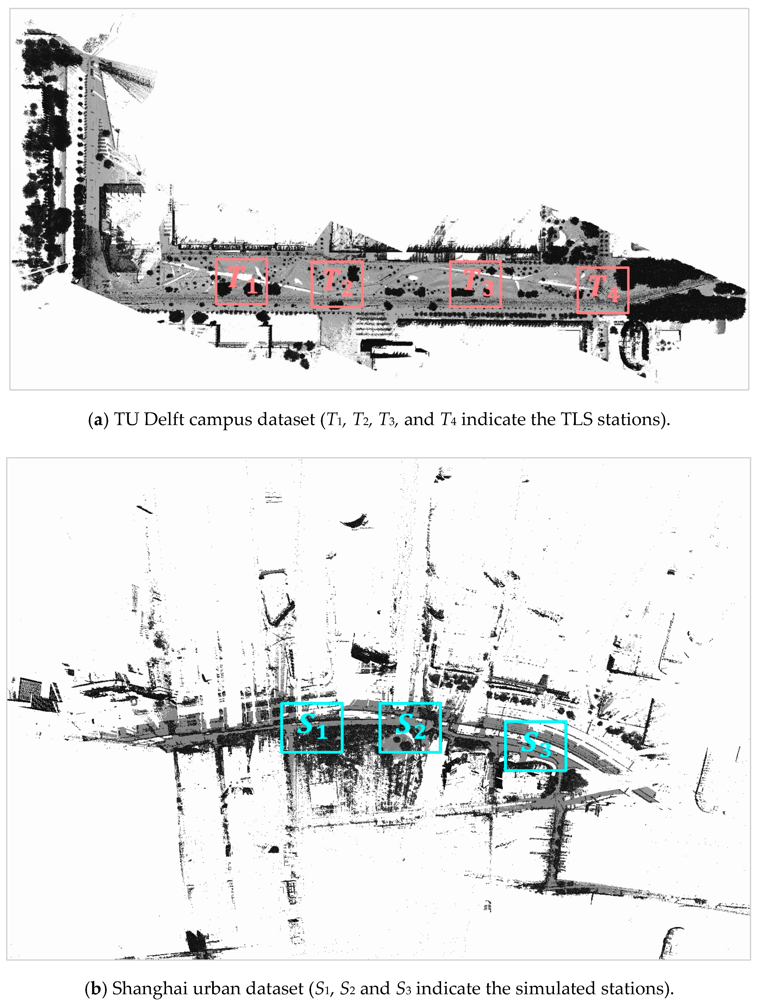
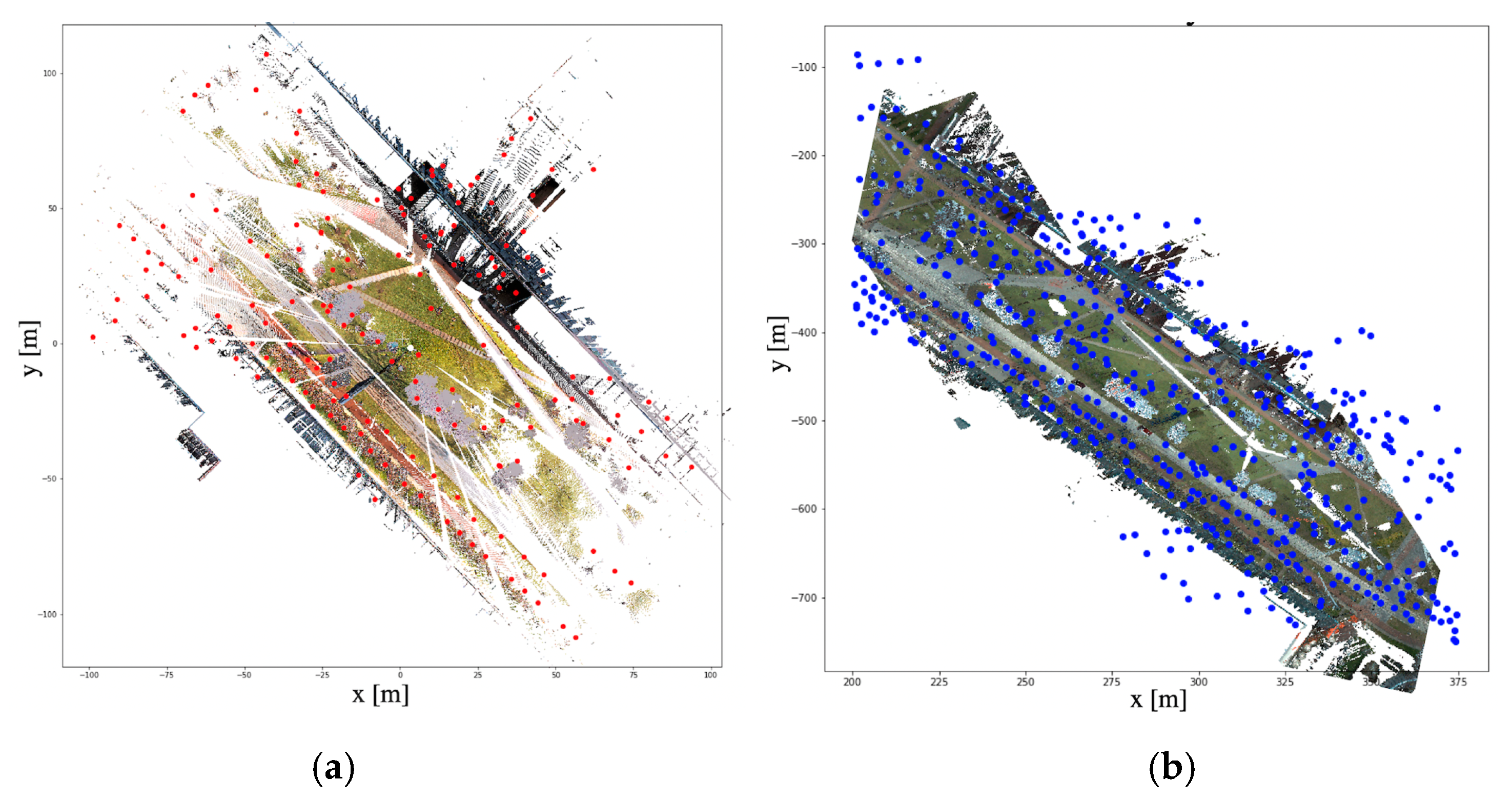
TU Delft campus dataset was acquired using Fugro Drive-Map MLS system with Riegl VQ 250 scanner, and Leica P40 TLS system mounted on a stationary tripod. A total of four TLS stations were set up and each scanning station covers an area with a radius about 200 m. Elapsed time between TLS and MLS data acquisition is about 4 years, where there are lots of constructions and vegetation change posing challenges for the localization. Additionally, for Shanghai urban dataset, Optech Lynx HS300 mounted on a vehicle was used to collect the environment along a street. The scanning routine is about 4.6 km, with lots of moving objects (e.g., cars and pedestrians) passed by during the acquisition. The detailed description of used laser scanners and datasets are listed in Table 1 and Table 2, respectively. Figure 1 shows the top distribution views of static TLS stations and MLS reference datasets.

Table 1.
Specifications of used laser scanners.

Table 2.
Description of Experimental datasets.

Figure 1.
Top distribution views of static TLS stations and MLS reference datasets.
4. Methods
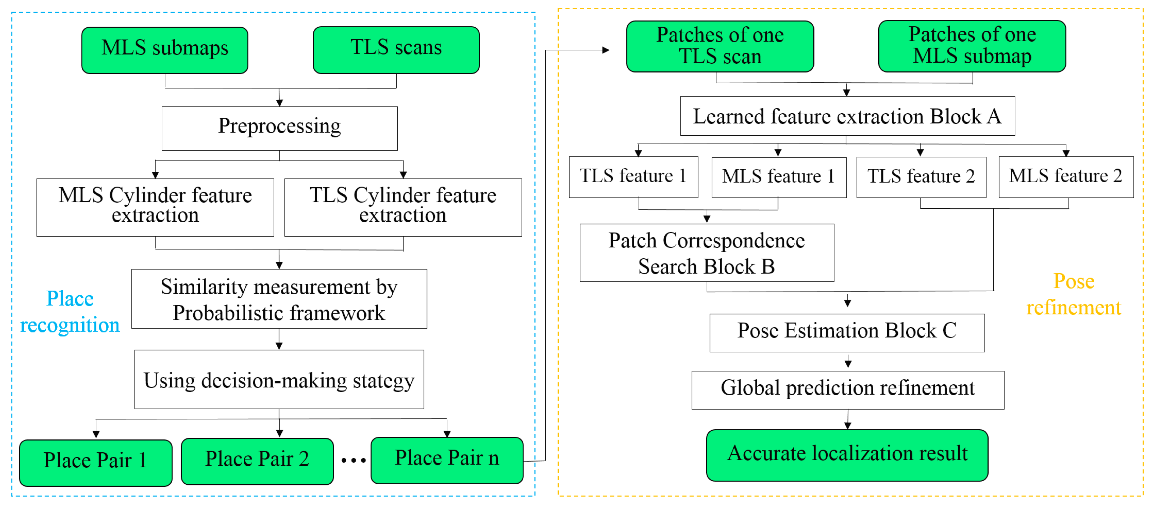
The proposed method encompasses two components: (1) place recognition and (2) pose refinement (Figure 2). In the place recognition, cylinder objects are extracted from both TLS and MLS data and similarity measurement based on probabilistic framework is proposed, which support to determine the related MLS scene for TLS scan, while in the pose refinement, three neural network blocks including learned feature extraction block, patch correspondence search block, and pose estimation block are designed to realize accurate localization of TLS in MLS data.
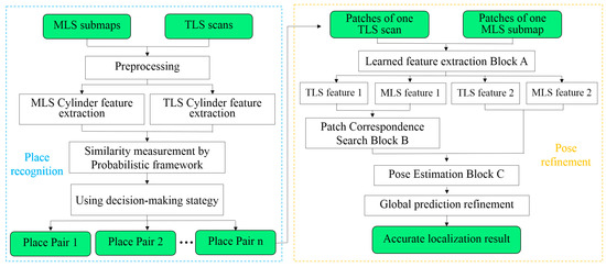
Figure 2.
Workflow for deep localization of TLS in MLS data.
4.1. Cylinder Object-Based Place Recognition
As MLS data used in this study consist of massive point clouds of objects along a routine, three objects (e.g., street pole lights, tree trunks and pillars) having parts of their geometry similar to cylinder-like objects, which are selected as feature primitives for place recognition. That is based on observing a typical urban scene always has cylindrical objects along a routine direction, which are relatively stable over time and can be easily scanned due to their distribution along a roadside although they may be partially blocked.
4.1.1. Cylinder Features Extraction
As complete building façades are not always visible in both TLS and MLS datasets due to limited scanning ranges and occlusions. To improve a correct matching ratio, cylinders near buildings are excluded. This section presents a framework to extract cylinder-like objects along the road as follows:
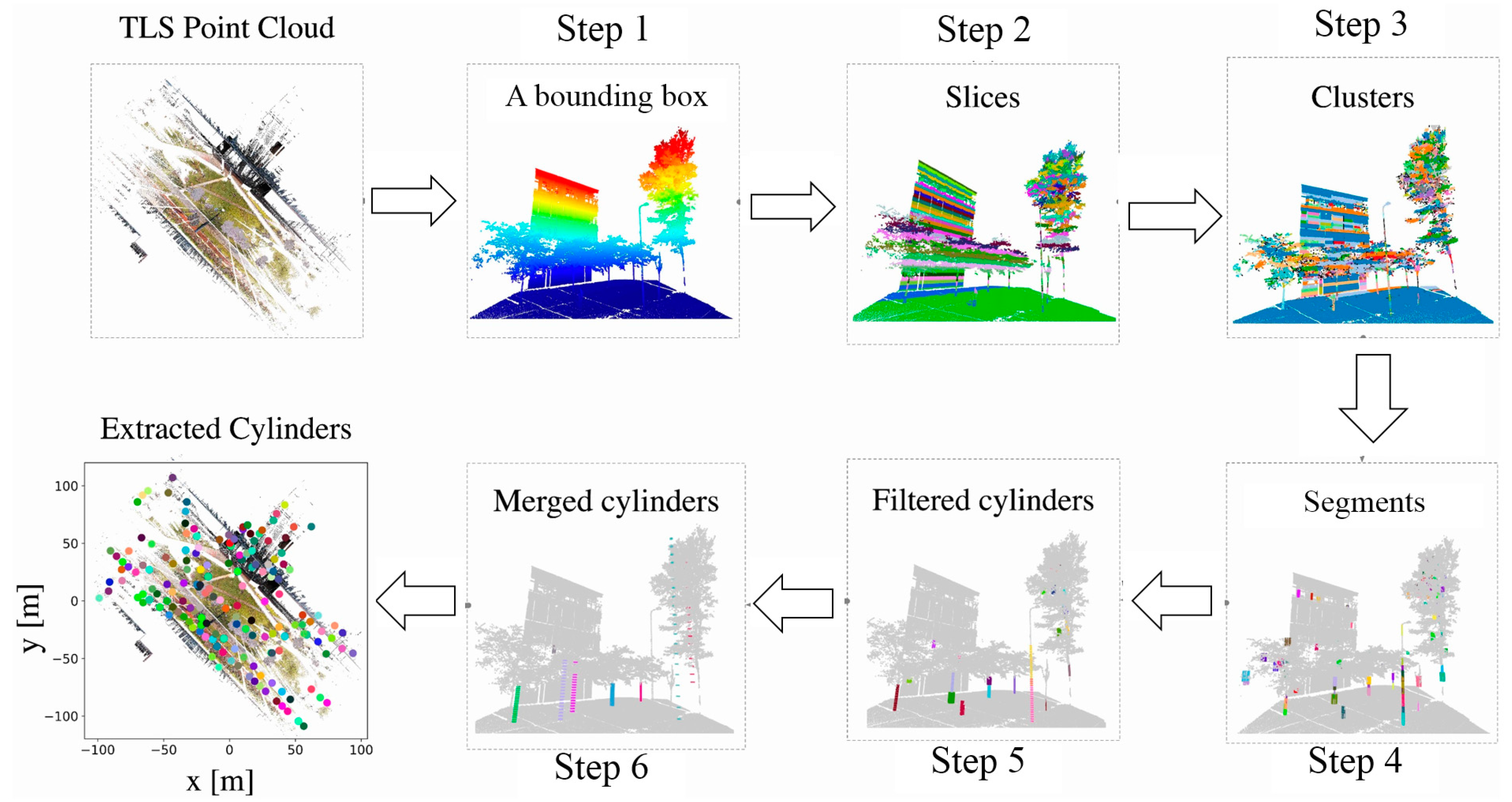
Step 1. All data are divided into 2D cells in the horizontal plane with different predefined cell sizes. Cell sizes of 5 m × 5 m and 20 m × 20 m are used for cylinder extraction and building façade.
Step 2. The point cloud within each cell is sliced along the z axis with a predefined slice thickness (e.g., 0.3 m). Then, the Connected Component Labeling [36,37] algorithm is employed to group the points within the slices into a set of clusters.
Step 3. To get complete clusters, the adjacent clusters are merged, if the horizontal distance between centers of two clusters are no larger than the threshold (e.g., smaller than 1.0 m), and their longest distances to the centers are similar (e.g., the difference smaller than 0.5 m).
Step 4. The point cloud of each cluster is projected onto the horizontal plane, and cylinder objects and building façades, respectively appear as circles and multiple line segments. These objects can be, respectively, determined by circle and line fitting algorithms [38,39]. Similar to Step 3, adjacent segments along a vertical direction are merged and incorrect segments caused by canopies are removed.
Step 5. The minimum distance between each extracted cylinder and the façade line is computed. To ensure a high correct matching ratio, the cylinders are removed if their distances less than the predefined threshold, which is empirically selected as 0.2 m in this study.
Step 6. In order to make each cylinder more distinct, cylinders within a radius (e.g., 5 m) in a vertical direction are merged to form a new cylinder.
According to the steps above, all cylinders from a TLS scan and a typical MLS scene can be extracted. The workflow is shown in Figure 3.

Figure 3.
Workflow of cylinder extraction, including intermediate results.
4.1.2. Probabilistic Framework for Similarity Measurement
This section presents a method to estimate the similarity between cylinders in target MLS scenes and those in source TLS scans. A probabilistic method is selected because it is suitable for the place recognition purpose due to the soft assignment strategy applied. The proposed methodology is briefly as follows.
In this work, a Gaussian Mixture Model (GMM) is used to describe the distribution of TLS cylinder points in a Euclidean space (Equation (1)).
where is the weight function for each cylinder in a TLS scan, Ns is the number of cylinders in the TLS scan, D and are, respectively, dimension and variance of the cylinder. By employing Coherent Point Drift (CPD) [33], the objective function is expressed in Equation (2):
where , Nt is the number of members in the target. The objective function is further maximized by expectation maximization (EM) algorithm to estimate rotation matrix R and translation vector T (Equation (3)).
Next, the estimated R and T are used to transform the cylinders in a source to get a virtual target. A similarity metric p describing the degree of overlap between the true target and the virtual target is expressed in Equation (4).
where t and t′ are, respectively, centers of true and virtual targets on a horizontal plane, is the Euclidean distance between two centers, Tdis is a distance threshold, which is chosen as 2.0 times of the cell size for cylinder extraction (introduced in Section 4.1.1).
In addition, to remove incorrect pairs and improve the matching stability, a mean distance is also defined (Equation (5)).
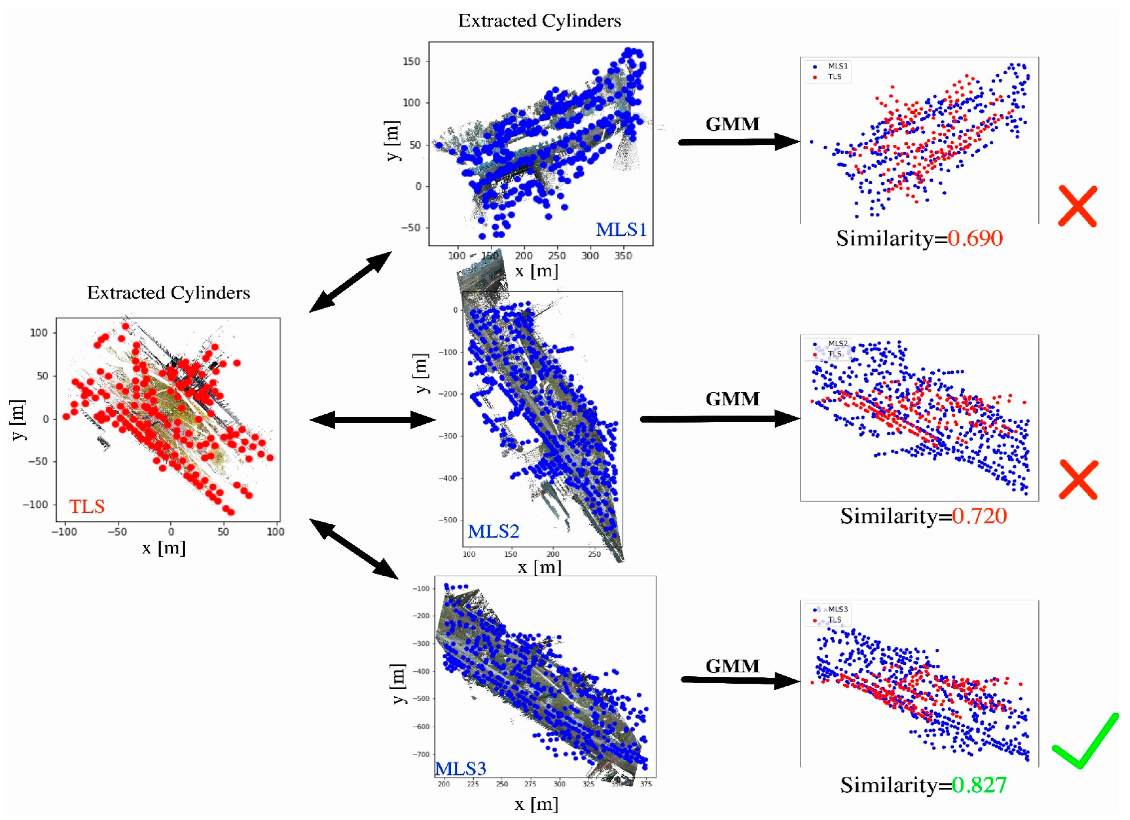
An example of a similarity measurement is shown in Figure 4.
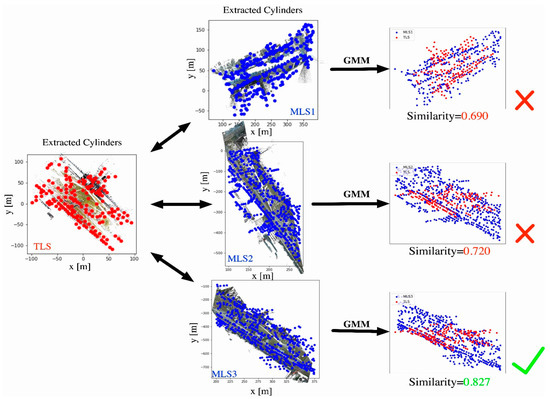
Figure 4.
An example of similarity estimation by probabilistic estimation between TLS and MLS (red and blue dots, respectively, represent TLS and MLS cylinders).
4.1.3. Decision-Making Strategy
Based on the estimated similarities between target MLS scenes and source TLS scans, a reliable matching strategy is required to obtain global optimum mapping pairs of MLS scenes and TLS scans. To fulfill this objective, a decision-making strategy is proposed as follows.
Step 1—Outlier removal: A pair of cylinders in MLS scene and TLS scan is considered as outlier if the similarity and distance between them is smaller and larger than the predefined thresholds, respectively. Considering the extraction errors, the similarity and distance thresholds are empirically selected as 0.6 and 10 m. The outlier pair is then removed and labeled as non-matching.
Step 2—Most dominance searching: This step is designed to determine the most likely pairs of MLS scenes and TLS scans. If we have N1 cylinders in TLS scans and N2 cylinders in MLS scenes, then for each cylinder in TLS scan, N2 cylinders in MLS scenes are candidates. The process starts to compute the difference ∆ (dominance) between the first two largest similarities. The MLS scene with the largest ∆ is selected as its correspondence.
Step3—Deactivation: If a correspondence is decided, the other candidates is labeled as non-matching.
Repeat above step 2 and 3 until all possible correspondences are estimated.
4.2. Deep Learning-based Pose Refinement
Considering characteristics of urban environment, a point cloud is down sampled to voxels with the voxel size of 5 m × 5 m × 3 m to generate patches as input data for pose refinement, with 256 points each. A patch randomly represents parts of TLS or MLS point clouds. A batch in the proposed neural network consists of several patches instead of one patch because we want to minimize the impact when the patches in the source obviously differs from that in the target because of temporal change or occlusions during data acquisition.
4.2.1. Patch-based Neural Network for Pose Refinement
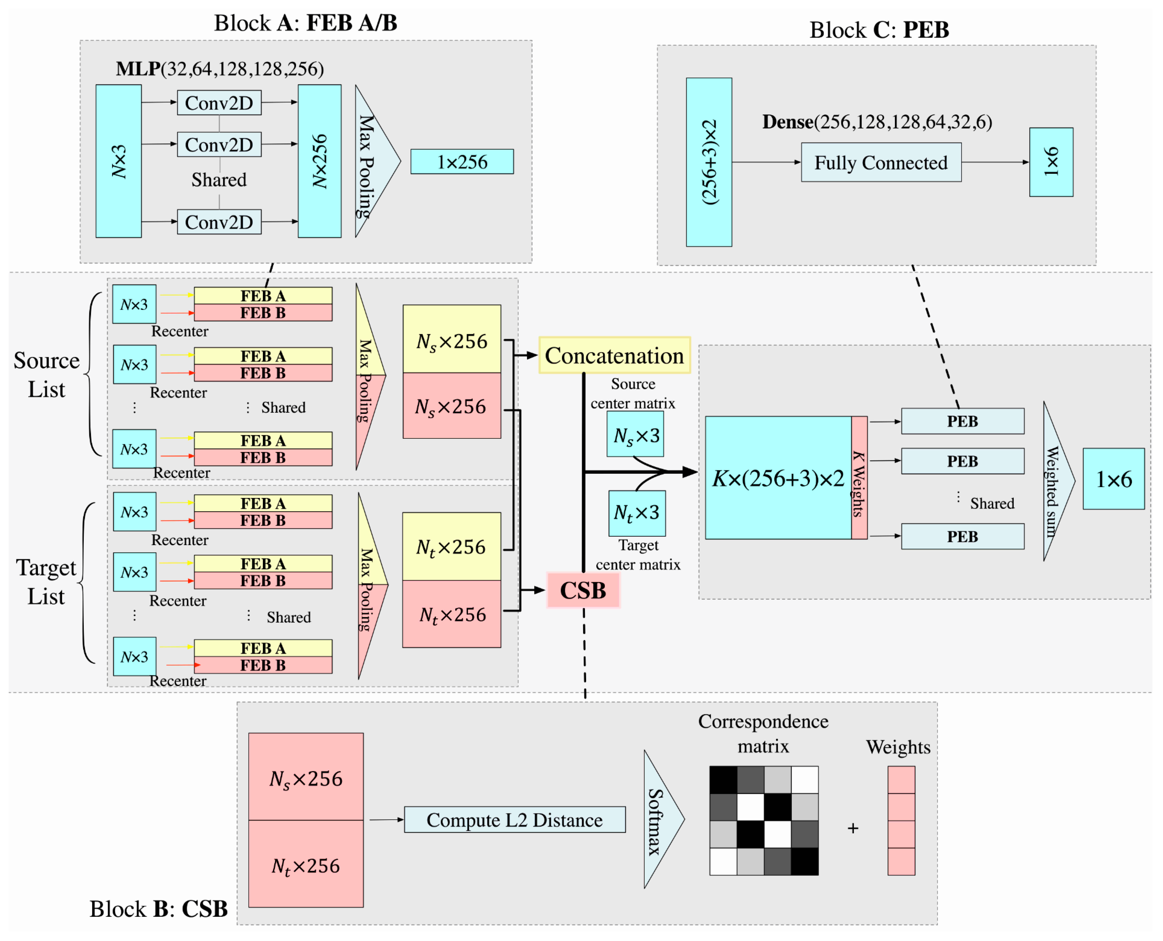
This section represents an accurate registration, which tunes the place recognition result by a patch-based neural network, as shown in Figure 5. Based on the result of place recognition, pairs of template MLS and source TLS point clouds can cover the same area obtained. For one pair, the patches retrieved from a template MLS scene and a source TLS scan form the target and source lists. As shown in Figure 5, both source and target lists go through three main blocks: block A—the feature extraction (FEB), block B—the patch correspondence search (CSB), and block C—the pose estimation (registration) (PEB).

Figure 5.
Overview of the patch-based neural network for pose refinement.
We designed two FEBs in block A, namely FEB A and FEB B. They have the same structure of network but are used for different purposes, in which FEB A and B are, respectively, for block C and B. To make it concise, taking FEB A as example, we designed the following steps. Firstly, we use centralization for each patch to make it translation invariant, the input list is shown as:
A five-layer MLP with dimension (32, 64, 128, 128, 256) is applied for each patch to summarize 3D coordinate information into 256 features for each point. Next, for each feature space within a patch, a max pooling process is used to keep the feature with the largest value and to form 256 features for this patch as patch features. After MLPs and a max pooling process, all features of patches in the source list or the target list are concatenated. When length of both source list Ns and target list Nt are equal to Nnn for each batch, in which Nnn = 10 in this study, an output is a (10, 256) matrix, which is shown as the red part in FEB in Figure 5.
In addition, the main purpose of Block B is to match patch correspondences between the source and the target lists based on invariant patch features. Block B is designed as follows. L2 distance is selected to compute feature distances between patches in the source and target lists (Equation (7)),
where fsource and ftemplate are the learned feature vectors of patches.
For all patches from the source and target lists, a feature distance matrix can be calculated. A small L2 distance indicates high similarity between patches. A Softmax function is employed to further normalize the feature distances (Equation (8)):
where and is a threshold for feature distance. In this paper, is decided by a validation set after training.
After retrieving the correspondence matrix, a list of correspondences is obtained by selecting the target patch with the largest possibility in the source patch (Equation (9)):
, where the ith patch in the source list and the jth patch in the target list representing most possible corresponding patch. The corresponding L2 feature distance vector of Equation (9) is written as:
To improve the stability of matching, we introduce weight for each feature distance vector to compensate for the differences between patch correspondences (i.e., density variations, noise, and data missing). We apply Softmax for vector dCrsp and the output value is used as the weight for each correspondence, which is shown as the right vector in CSB in Figure 5. Noticeably, this weight is used to make most similar patch corresponding pairs more dominant, and to accelerate the training process. For example, if a patch correspondence has a low L2 feature distance, it will dominate the output. If this pair has good quality of the output (i.e., smaller loss function value), then parameters will be tuned by generating a larger weight. Finally, the learned features for each patch correspondence and the patch centers are combined to form a concatenated feature vector with length (256 + 3) × 2, shown as the left vector in PEB in Figure 5.
After block A and block B, a 10-weight vector ω and a concatenated feature matrix are generated. For each correspondence, six fully connected layers in block C with dimension (256, 128, 128, 64, 32, 6) are applied to summarize these features to the final six pose parameters ξ. The final pose parameters are computed as given in Equation (11).
The predicted rotation matrix and translation vector are computed based on pose parameters.
4.2.2. Design of Loss Function
Loss function is an important component for a training process. It describes difference between the predicted result from a trained neural network and the true value. Different loss functions may train totally different neural networks, as a neural network is tuned by the gradient of loss function in each epoch. In this implementation, the loss function consists of three parts: a rotation loss , a transformation loss , and a labeling loss (Equation (12)):
where and are balancing coefficients (). The rotation loss is defined as the root mean square error (RMSE) between the predicted rotation matrix and the truth . We compute the RMSE between and the corresponding identical matrix to ensure the predicted rotation matrix always invertible (Equation (13)):
In addition, a transformation matrix is computed to combine the rotation and translation loss, in which the transformation loss is similar to the rotation loss (Equation (14)).
where and are the predicted and the true transformation matrix, respectively, and is a 4 × 4 identical matrix.
Inspired by a cross entropy, which is computed by comparing the probability between each predicted result and each class in classification, we design a labeling loss with Softmax. By minimizing it, the probability of true correspondences in the correspondence matrix must be close to 1. The labeling loss is defined as given in Equation (15):
Here, and are predicted and true correspondence matrix, respectively.
4.2.3. Global Prediction Refinement
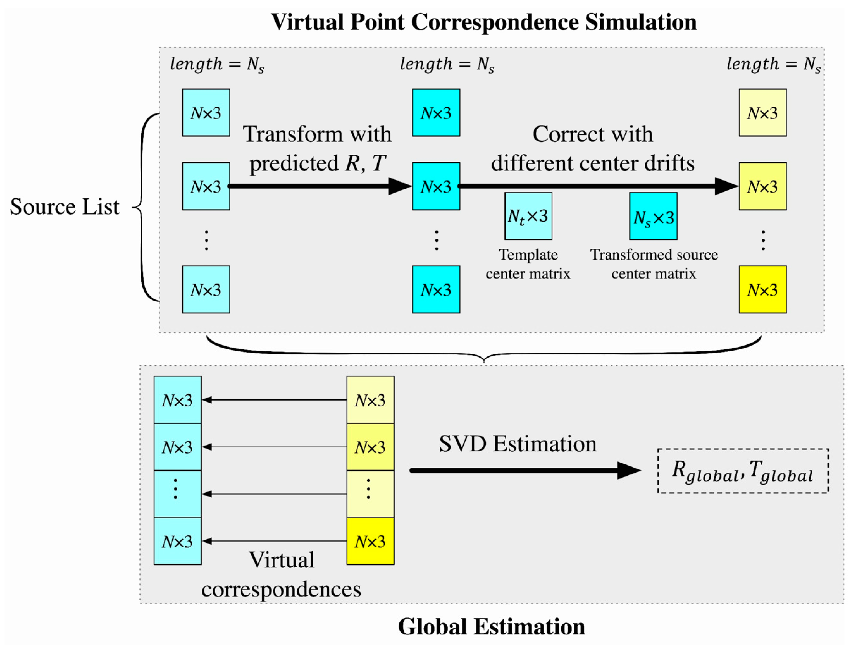
Even for point-based networks designed for simple objects, the issue of obvious transformation offsets comes up sometimes [27]. Therefore, it is huge challenge to train a neural network accurately for point cloud registration from large-scale scene because the scene is more chaotic and contains various objects. To solve this problem, we propose a global refinement method consisting of two steps: virtual point correspondence simulation based on the center drift correction, and global estimation, as shown in Figure 6.

Figure 6.
Schematic diagram of the proposed global refinement method.
Differing from point-to-point iterative closest point (ICP) [40] and DeepVCP [24], which simulates virtual correspondences under a voxel-based convolutional neural network, we simulate virtual point correspondences for every point in source patches based on the predicted rotation matrix, the predicted translation vector and different center drifts, as the upper part of Figure 6. The process works directly with the points without requiring neighboring searching, which can reduce significant executing time.
For one patch in the source list where there are Nnn patches, virtual corresponding points for this patch are computed by adding the center drift for this patch to the predicted patch , to from a pair matrix , as:
For each patch , the predicted rotation matrix is the same as , while the predicted translation vector varies, which depends on the center drift . By doing this, we have Nnn different translation vectors after virtual point correspondence simulation.
After generating virtual correspondences, a global estimation is applied for all point correspondences from Nnn different patches, where Nnn = 10 is the length of input source or target list. Based on SVD decomposition for 3D point least square estimation [41], which estimates a rotation matrix and a translation vector by SVD decomposition for a matrix of points and their correspondences, a global rotation matrix and a global translation vector for all points from different source patches within the same batch are retrieved, as the lower part of Figure 6 shows. Finally, the pose refinement is obtained by getting a transformation matrix .
5. Experimental Results
5.1. Experimental Setup
The implementation details of the experiments, including the data preparation, evaluation criteria and implementation environment are described in this section.
5.1.1. Data Preparation
As mentioned before, TU Delft campus and Shanghai urban datasets were used in the experimental tests, in which details of two datasets are introduced in Section 3.1. For the TU Delft dataset, source and target patches are randomly generated from TLS scans and corresponding MLS scenes, respectively. For the Shanghai dataset, both source and target patches are randomly generated from the MLS point clouds. The TU Delft dataset uses both TLS and MLS point clouds in every pose refinement experiment. The Shanghai dataset only uses MLS point clouds in evaluation. Details of data for training are shown in Table 3. In addition, a rotation range and a translation range are an angle range and an offset range, w.r.t. the (x, y, z) axis, respectively. The Shanghai dataset has a larger rotation range w.r.t. the z axis and a larger horizontal translation range since less noise introduced. These settings aim to evaluate pose refinement at a larger scale.

Table 3.
Description of data for training and evaluation.
5.1.2. Evaluation Criteria
- Confusion matrix w.r.t. patch and batch
To evaluate the performance of patch correspondence matching, confusion matrices with respect to patch and batch is defined. There four types of elements in a confusion matrix named true positives (TP), false positives (FP), true negatives (TN) and false negatives (FN) (Equation (17)). After the patch correspondence search block (CSB), in a single batch, we get Nnn pairs of for the ith patch in the source list and its most possible corresponding patch, the jth patch in the target list. TPp, FPp, TNp and FNp are defined as:
where r is a threshold and r = 0.95 is suggested, C and Ctrue are the predicted and the true correspondence matrix defined in Equation (8), respectively. Similarly, for a batch bk (1 ≤ k ≤ B), B is the number of input batches. TPb, FPb, TNb and FNb are defined as:
where is a threshold, and is suggested. TPp, FPp, TNp and FNp are computed by patch pairs in batch bk. TPb, FPb, TNb and FNb describe the performance of results computed based on batches. For example, if the number of patch positives (TPp + FPp) in a batch is smaller than 5, this batch is not used in PEB because there are less patches to apply the global refinement that led to it is not reliable.
- Precision–Recall Curve
To evaluate the performance of patch correspondence matching, a precision–recall (PR) curve is used to show a tradeoff between the precision and the recall under different thresholds. Both precision and recall are computed from a confusion matrix. A high precision indicates there are less FP and a high recall relates to less FN, but it is hard to ensure a high level of both precision and recall in most circumstances, so we need to make a balance between precision and recall to select a proper threshold. In order to represent the matching result more intuitively, a (1-precision)–recall curve is plotted in our experiments.
In general, the patch precision relates to a correct ratio of patch correspondence estimation, and the patch recall indicates a percentage of patch correspondences correctly estimated. The batch precision expresses an accuracy of estimated pose parameters, and the batch recall indicates the percentage of reliable batches.
5.1.3. Implementation Environment
The training process is run on TU Delft high performance clusters (HPC) using a CentOS 7 Linux distribution, with 1080Ti geographic processing unit and programming languages including Pyhon 3.7.7, TensorFlow 2.3.0, open3d 0.9.0. Other experiments are processed under Mac OS Catalina 10.15.6, with 2.9 GHz Quad-Core Intel Core i7 processor and 16 GB 2133 MHz LPDDR3 memory. The compiler is Jupyter Notebook 6.0.3 for python3.
5.2. Place Recognition Results
This section presents extracted cylinder features, correspondences estimation and place recognition results.
5.2.1. Cylinder Feature Extraction Results
Using the feature extraction method in Section 3.1, cylinder features were extracted from TU Delft campus dataset. Results of object extraction is summarized in Table 4 and Figure 7, which were based on TLS scans (totally 4 scans) and MLS scenes (totally 5 MLS scenes). Table 4 shows that large number of cylinders (totally 3179 cylinders) and many façade lines (totally 660 lines) were extracted, which ensures the sufficient quantity of corresponding cylinder pairs in the overlapping area. The right column in Table 4 shows that the correct extraction ratios of cylinders are more than 75%, ensuring the correct ratio of matching and making it suitable for the following probabilistic framework. Besides, a comparison to Table 2 shows that about 100 cylinders are extracted per million points from TLS/MLS point clouds at 0.1 m voxel down-sampling. It is more time consuming to extract features from the MLS point clouds due to their larger area and large number of voxels. Run time per million points of cylinder feature extraction is longer in TLS scans, about 10 s compared to 5 s in MLS scenes. The reason for this longer run time is that there is less information of the facades but higher point density at canopies and terrain in TLS scans.

Table 4.
Extraction information of MLS scenes and TLS scans.
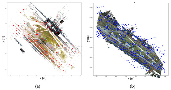
Figure 7.
An example of extracted cylinders in one TLS scan (a) and one MLS scene (b).
5.2.2. Recognized Results Based on Extracted Features
Based on the probabilistic estimation in Section 4.1.2, a similarity and a mean distance for each pair of cylinders in TLS and MLS point clouds are computed based on Equations (4) and (5). Results are shown in Table 5, in which values with upper index a represent outliers that have the similarity and mean distance are smaller and larger than corresponding thresholds, respectively (Section 4.1.3), values with upper index b represent ambiguities which have more than one matching pairs (i.e., more than one candidates can meet the thresholds) e.g., (TLS1, MLS2) and (TLS3, MLS4), and values with upper index c represent the dominant solutions that have larger similarity than other pairs e.g., (TLS2, MLS3). Due to rough cylinder extraction and additional spatial-temporal change between TLS and MLS point clouds, only two correspondences are used in dominant solutions. Thus, a decision-making strategy needs to be applied to extract as many correct corresponding pairs as possible.

Table 5.
Computed similarity (a.u) and mean distance (m) between TLS and MLS cylinders.
The results of the decision-making process are shown in Table 6, in which Table 6a shows the outliers are removed, ambiguities and dominant solutions are found and reserved; Table 6b–d show the most dominant solution was found step by step until all possible pairs are decided. Table 6 shows that the correct places (e.g., (TLS1, MLS2), (TLS2, MLS3), (TLS3, MLS4), (TLS4, MLS5)) can be recognized, demonstrating the effectiveness of the proposed place recognition method.

Table 6.
Decision-making process and results (x, 0 and 1 indicate an undecided pair, a non-matching pair and a matching pair, respectively).
5.2.3. Overview of Place Recognition
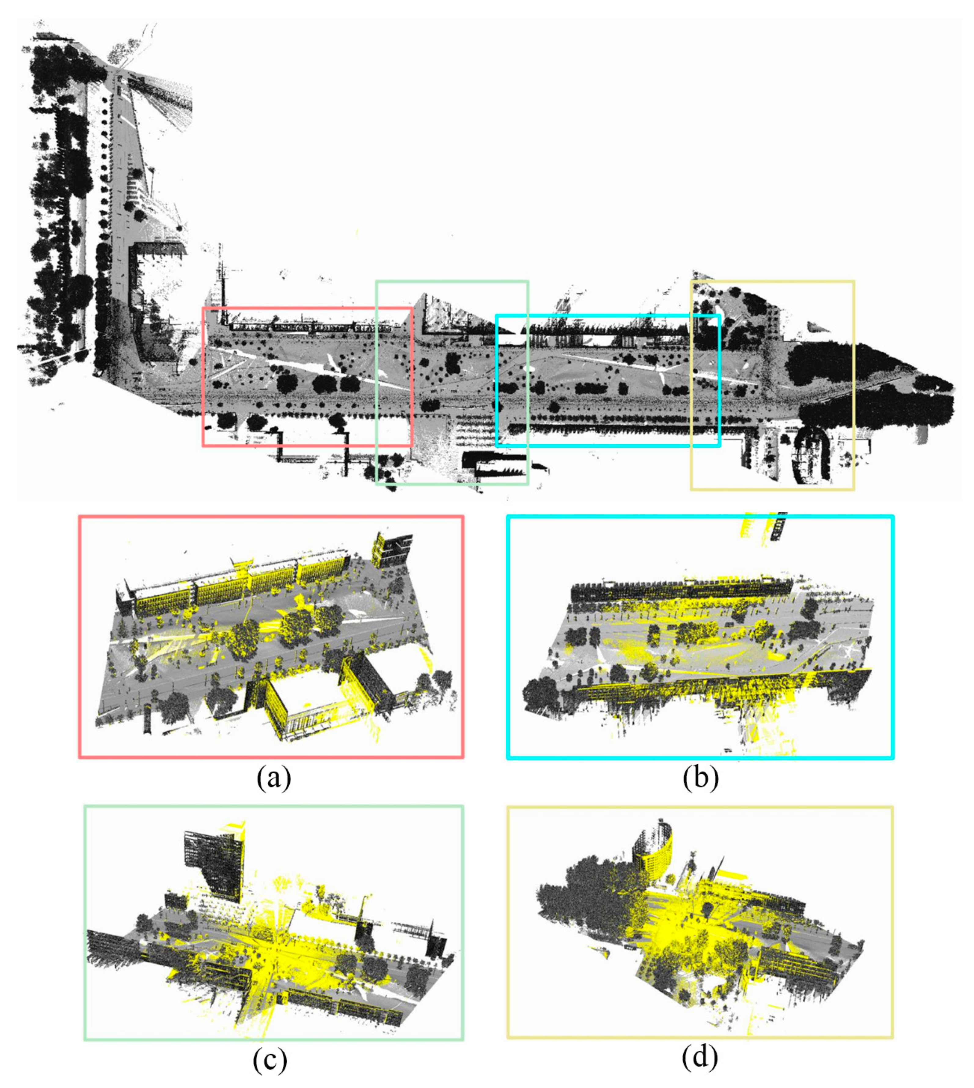
Final correspondences between TLS scans and MLS scenes can be obtained on the place recognition framework in Section 4.1. An overview of recognized correspondences transforming from TLS scans to MLS scenes are shown in Figure 8. A success rate of place recognition is 100% in the experiments (i.e., all the TLS scans are related to correct MLS scenes successfully). It is worth noting that lots of new vegetation appear during the interval between MLS and TLS collection. Initial transformation varies in different correspondences, which depends on results of GMM probabilistic estimation. Figure 8a shows a large rotation angle (about 25 degrees with respect to the z axis), and Figure 8d shows a satisfying result with a small rotation angle (about 5 degrees with respect to z axis) between the transformed TLS scan and corresponding MLS scene. It is because the distribution and extraction quality of cylinders affect the place recognition. However, correct MLS scenes can still be recognized, demonstrating the stability and effectiveness of the proposed method.
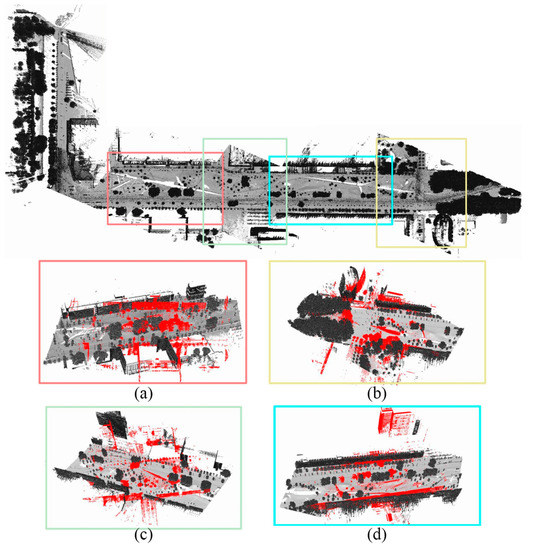
Figure 8.
Overview of place recognition results: (a) recognized MLS place of T1 station; (b) recognized MLS place of T4 station; (c) recognized MLS place of T2 station; (d) recognized MLS place of T3 station.
5.3. Pose Refinement Results and Evaluation
5.3.1. Performance of Thresholds in the Correspondence Search Block
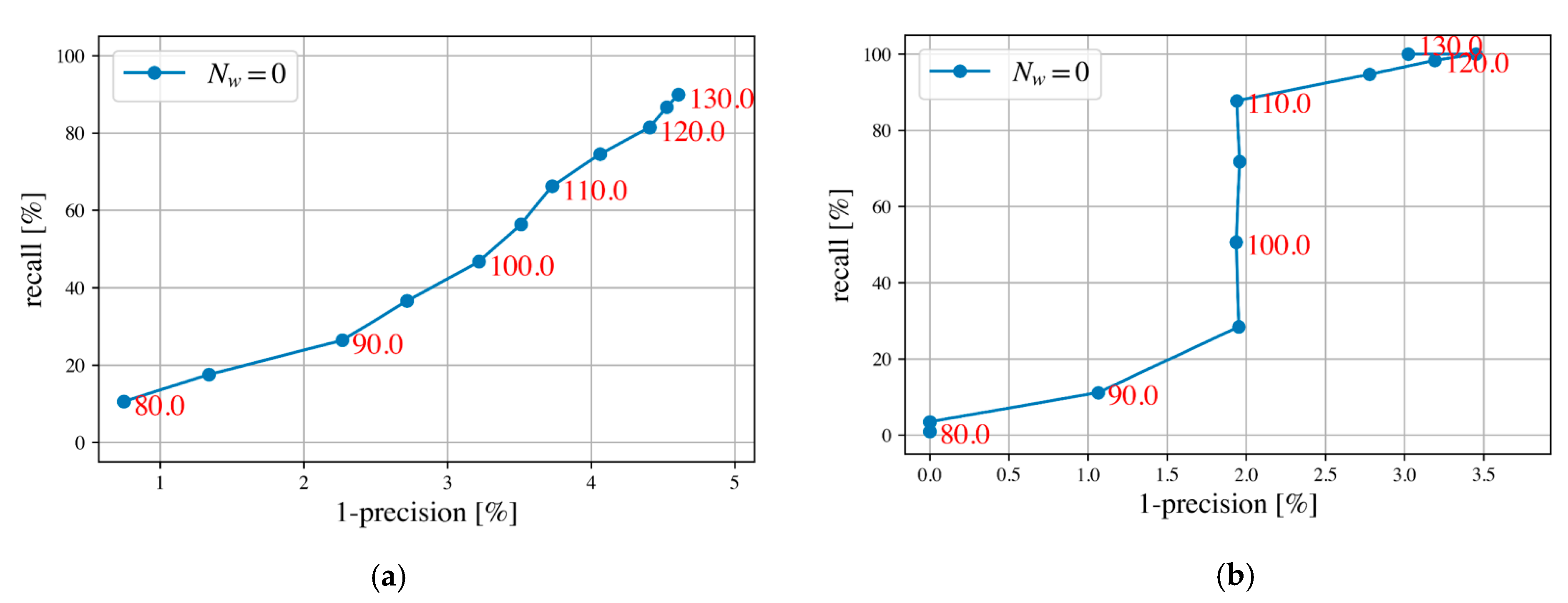
Different distance thresholds of in Equation (8) are given different recall and precision values in the PR curve, which depends on training epochs and hyperparameters (Figure 9). This experiment assumes that patches are one-to-one corresponding between source and target lists. Validation-based TU Delft holdout set was used to show the performance of different w.r.t. patch and batch (Figure 9), in which values represent the threshold of the L2 feature distance and Nw = 0 indicates source patches and target patches are one-to-one corresponding. Moreover, Figure 9a shows an approximate lineal trend under different thresholds between patch precision and recall, in which a high precision corresponds to a low recall. In other words, a small leads to a high precision but a low recall. In Figure 9b, there is a sharp jump in the recall for four thresholds 95.0, 100.0, 105.0 and 110.0, which indicates these four thresholds do not affect batch precision. In general, it is a tradeoff between precision and recall to select a proper , and although we prioritize a precision, the threshold is selected to make sure both patch and batch recall higher than 40%. Finally, we choose = 100.0 as the feature distance threshold, since this results in a recall w.r.t. patch or batch of nearly 50%, and a precision above 95% in the validation holdout set.
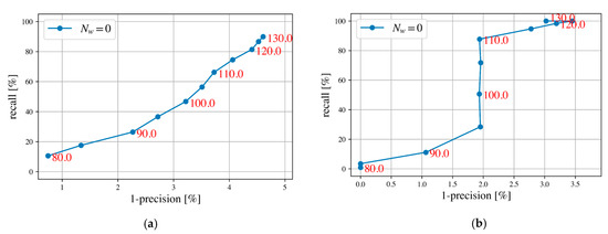
Figure 9.
Precision–recall (PR) curves computed for the TU Delft validation holdout dataset (red numbers represent the thresholds of L2 feature distance): (a) PR curve w.r.t. patch and (b) PR curve w.r.t. batch.
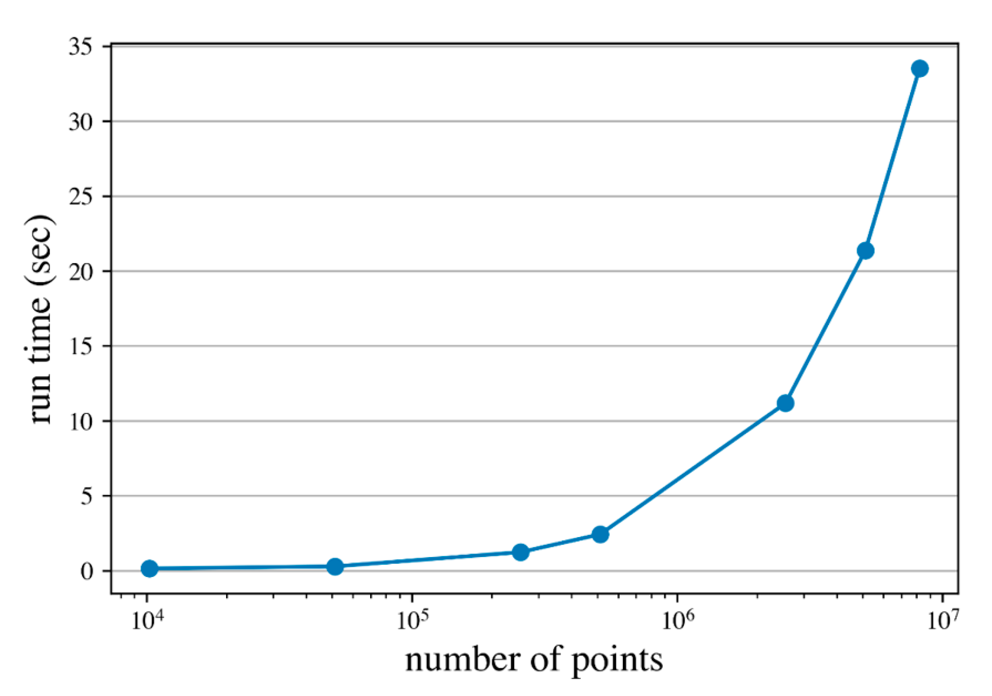
Run time of CSB with respect to different numbers of points is shown in Figure 10. Processing time of TU Delft test set takes about 34 s for more than 8 million points, with 10 patches in a single batch.
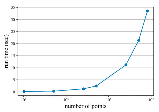
Figure 10.
Run time of the patch correspondence search block under different number of points processed.
5.3.2. Overview of Pose Refinement Results
After training and validation, pose parameters for each correspondence of place recognition results were estimated based on a trained neural network for pose refinement. Transformed TLS scans of place recognition results were achieved by a transformation matrix computed from the extracted pose parameters. An overview of pose refinement results is shown in Figure 11, which is connected to place recognition results in Figure 8. After the pose refinement, four corresponding pairs show accurate results (the rotation angle w.r.t. the z axis is smaller than 1.0 degree and the horizontal translation offset is smaller than 1.0 m) in comparison to place recognition results. It proves our potential registration neural network can give an initial alignment of the place recognition, where point clouds from TLS and MLS are close. Moreover, although TLS scans and MLS scenes are collected at different times that differences exist between them, and the scenes are chaotic that contain various objects, the pose refinement as long as patch corresponding pairs are correctly estimated, where the rotation angle w.r.t. the z axis between transformed TLS scans and corresponding MLS scenes is smaller than 30.0 degrees and translation offsets are not obvious (smaller than 5.0 m) after the place recognition.
6. Discussion and Analysis
6.1. Evaluation of Correspondence Search Block
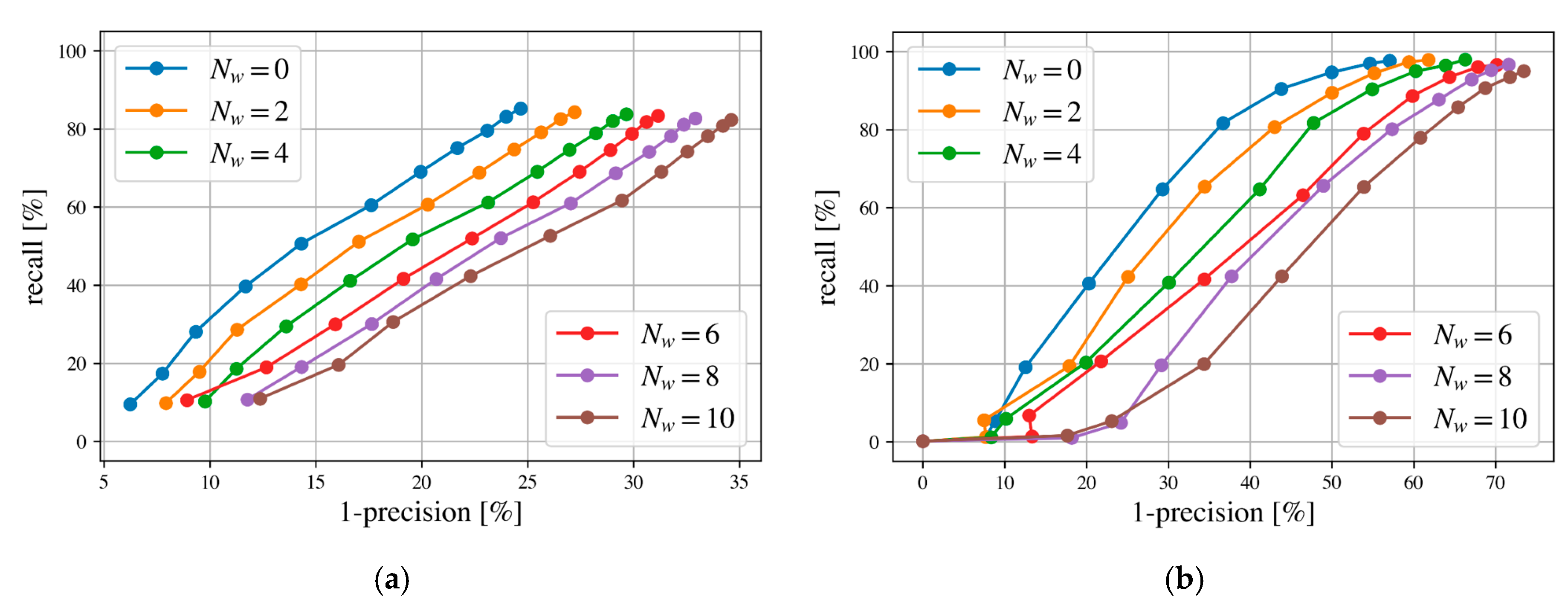
For the validate-based TU Delft holdout set, the precision and recall w.r.t. batch or patch are high (precision > 95% and recall∼50%) when = 100 was selected. Moreover, to evaluate the performance of the precision and recall based on TU Delft test set, apart from the case of one-to-one matching between source and target patches for each target batch random patches (e.g., 2, 4, 6, 8, 10) were added from other target batches. Two patches were randomly added to a batch, and then two source patches are incorrectly matched to one of the random patches. Results of PR curves for different numbers of random patches are shown in Figure 12 for the TU Delft test dataset.

Figure 12.
Precision–recall (PR) curves computed for the TU Delft test dataset, with Nw random patches added: (a) PR curves w.r.t. patch (b) PR curves w.r.t. batch.
The precision w.r.t. patch and batch decreases significantly at TL2 = 100, about 10% and 18% in TU Delft holdout set, respectively; however, the recall is still above 40%. Both patch and batch PR curves from different numbers of random patches show an approximate linear trend between precision and recall (Figure 12). A randomly added patch leads to a decrease of about 1.1% in the patch precision and about 2.2% in the batch precision. This decrease is caused by the similarity between a random patch and a true corresponding target patch, e.g., the similar appearance of the ground truth. The recall is less affected by random patches since there are many similar patches generated from canopies, buildings and roads in an urban area. Additionally, in order to decrease the impact of random patches on patch and batch precision, we need to avoid similar patches to be appeared in the same batch by controlling the input patches.
6.2. Evaluation of Pose Estimation Block and Global Prediction Refinement
CSB estimates corresponding pairs between source and target patches. In this experiment, assume there are 10 successfully estimated corresponding pairs. We cannot add errors to PEB as it is pre-trained. Errors are simulated during the virtual point correspondence simulation in the global refinement, by which the impact of errors on the global refinement for predicted results of PEB is evaluated. The list of n center offsets for n source patches is defined as:
where , , and Ns is the number of patches in the source list.
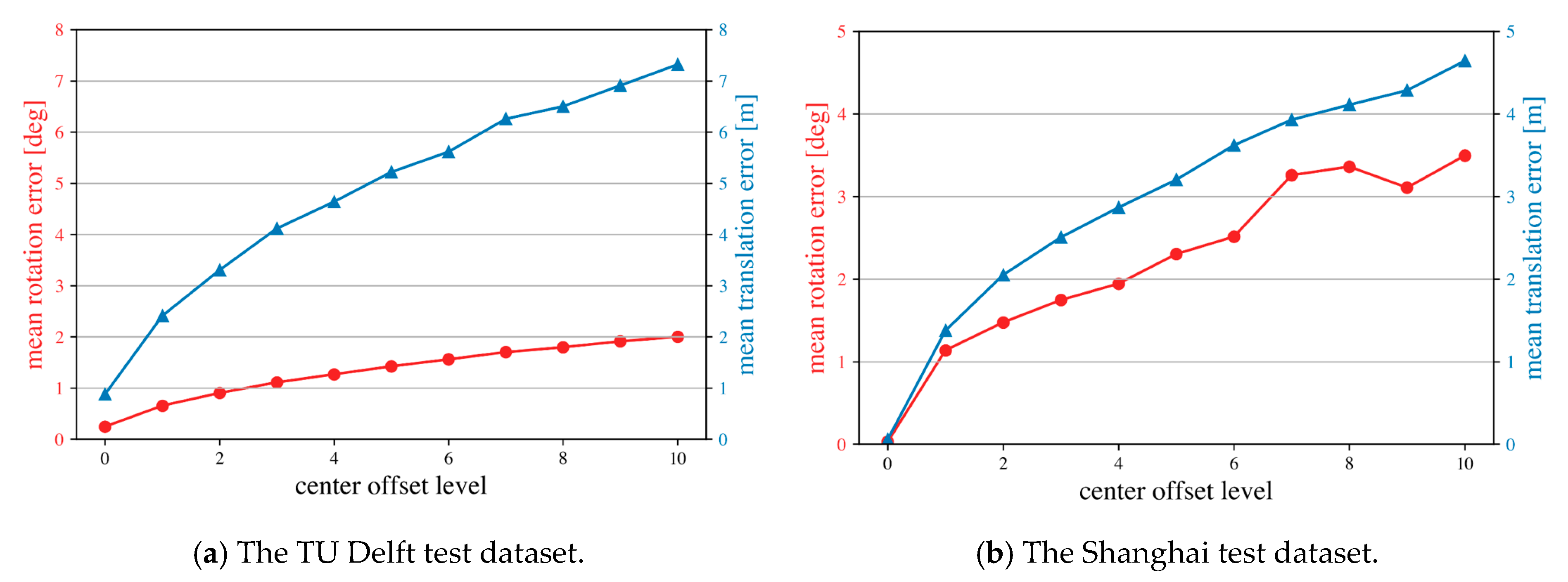
The length of the center offset list n is shown as the n center offset level as well. The mean pose error of 0 to 10 center offset level are shown in Figure 13. The Shanghai test dataset have a mean translation error smaller but a mean rotation error larger than those of the TU Delft test dataset at the same center offset level. Moreover, during the global refinement process, the correction of center drift strongly impacts the improvement of predicted results. The rate between maximum mean rotation error and the rotation range about the z axis is about 0.0666 and 0.0222 for the TU Delft and the Shanghai test dataset, respectively. This rate indicates that the fluctuation of the Shanghai test dataset is smaller than that of the TU Delft test dataset. The larger mean rotation error of the Shanghai test dataset is possibly caused by the larger rotation range. Generally, each increase of center offset leads to an increase of about 0.65 m and 0.45 m of the mean translation error, and 0.2 deg and 0.35 deg of the mean rotation error for the TU Delft test dataset and the Shanghai test dataset, respectively. The Shanghai test dataset has a better performance during the evaluation of PEB and the global refinement, as it always has the smaller mean translation error. Moreover, the Shanghai dataset only uses MLS point clouds, so source and target patches are less noisy. Finally, the performance of PEB and the global refinement for the TU Delft test dataset can be improved by filtering noise in input patches and need to be close between the source and the target.
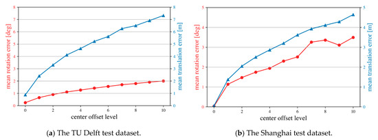
Figure 13.
Mean error of rotation and translation for different center offset levels.
6.3. Comparison between the Proposed Method and Traditional Methods
The performance of the proposed method was compared with traditional methods, in which four classical registration methods (i.e., point-based, plane-based, feature-based and probability-based methods) were used, with settings shown in Table 7. ICP_P2Po is the point-to-point iterative closest point (ICP) registration [40], ICP_P2Pl is the point-to-plane ICP registration [42], FPFH+RANSAC is random sample consensus (RANSAC) registration based on fast point feature histogram (FPFH) matching [34], CPD is rigid registration based on Gaussian mixture model (GMM) probabilistic estimation [33]. Moreover, two types of the proposed networks corresponding two sets of balancing factors (α, β, γ) (α = 100, β = 10, γ = 100 for network A; α = 100, β = 100, γ = 100 for network B) were also included to give results with and without the global refinement, which are shown as predicted network A/B, corrected network A/B, respectively. The comparison is measured through five metrics, namely: the mean and maximum error in rotation and translation, and the run time of processing 8 million points. Among them, mean translation error is calculated as a mean root mean square error (RMSE) between the sampling points of predicted patches and true patches. For each patch, 256 points are sampled and the mean point span is about 0.3m. The comparisons based on TU Delft campus data and Shanghai urban data are shown in Table 8 and Table 9, respectively.

Table 7.
Parameter setting for compared methods.

Table 8.
Error analysis of the TU Delft test dataset (Bolded values represent good performance achieved).

Table 9.
Error analysis of the Shanghai test dataset (Bolded values represent good performance achieved).
Table 8 shows that corrected Network A and B have a lowest mean rotation (0.24 deg) and translation (0.88 m) error, while run time is about 4.5 s per million points. CPD also has small mean pose errors (0.27 deg in a rotation and 0.95 m in a translation), but the method is time consuming with over 100 s per million points. This implies the CPD method is properly applied for a small sample dataset. Moreover, two ICP methods perform well with the max pose errors about 0.35 deg in a rotation and 1.76 m in a translation. Point-to-plane ICP registration is out performance to point-to-point ICP registration (about 200 s are saved during processing 8 million points). In terms of the failure of FPFH+RANSAC, it is due to the fact that the voxel cell of down-sampling of 1.0 m is too large to extract FPFH features, then extracted FPFH features are not reliable for registration. FPFH+RANSAC is time consuming with running time about 100 s per million points, so there is no need to repeat this experiment using dense point clouds, for example, point clouds with a 0.05 m voxel cell. Although Predicted Network A/B is the most efficient method (26 s of processing 8 million points), the mean pose error is relatively large (>5 deg in rotation and >5 m in translation) compared to other methods. This large pose error also indicates the point based neural network is hard to achieve a satisfying result (the mean pose error of <1 deg in rotation and <1 m in translation) for point cloud registration at a large scale, e.g., an urban environment. Overall, the ICP registration performs better at the max pose error, and a corrected neural network has a better result of the mean pose error, with high efficiency. Table 9 shows that the mean and the max pose error are all small for our neural network (0.03 deg of rotation and 0.06 m of translation in the mean pose error). This is because there are little differences between MLS scenes and simulated TLS scans in Shanghai urban data while the TU Delft campus data have significant differences since the elapsed time between its TLS and MLS data acquisition is four years, during which lots of vegetation changes occurred. Table 9 also shows that ICP and CPD registration methods cannot work because the large initial rotation range makes them fall into local convergence.
7. Conclusions and Future Work
Localization techniques offer to understand a surrounding environment by getting position information in a geographic reference map. Unfortunately, interruption of GNSS signal transmission, especially in urban scenes, exerts great influence on GNSS localization. 3D point cloud localization of TLS scans in large-scale MLS reference data are signal transmission free, which can afford detailed geographic information for lots of tasks especially in autonomous driving and robotics. This paper presents a novel deep localization method of TLS static scans in MLS point clouds of urban environment, divided by place recognition and pose refinement. Its performance is validated on two real-world urban datasets. Comprehensive experiments demonstrate that the proposed method obtains good performance in terms of accuracy, efficiency, robustness, and applicability, and outperformed some commonly used methods.
Although the proposed method can provide satisfactory results on urban datasets, it is susceptible to the incorrect patch pairs. If the segmentation information can be attached for each patch, the precision of CSB will be improved significantly. Another possible way is to find a resampling method to make resampled patches more distinct. As for the improvement of output of PEB, it is possible to add some complementary information, for example, features computed by traditional methods, to learned features, which can partially control the training process instead of a complete black box.
In the future, we will further improve the place recognition method. By extracting more common and descriptiveness geometric features, and improving the correspondence matching strategy, a more stable and accurate place recognition can be developed. On the other hand, we will also focus on the performance of deep neural network by designing a new input data unit to improve the descriptiveness and distinctiveness.
Author Contributions
Y.Z. designed the algorithms as described in this paper and was responsible for the main organization and writing of the paper. F.M., R.L., and L.T.-H. contribute to the conceptualization, data curation, and investigation. B.L. contributes to the data acquisition. R.L. and L.T.-H. revised the manuscript. All authors have read and agreed to the published version of the manuscript.
Funding
This research was funded by [National Science Foundation of China project under] Grant No. 41701529, and [OpenFund of State Laboratory of Information Engineering in Surveying, Mapping and Remote Sensing, Wuhan University] Grant No. 18S02.
Institutional Review Board Statement
Not applicable.
Informed Consent Statement
Not applicable.
Data Availability Statement
Not applicable.
Conflicts of Interest
The authors declare no conflict of interest.
References
- Drawil, N.M.; Amar, H.M.; Basir, O.A. GPS localization accuracy classification: A context-based approach. IEEE Trans. Intell. Transp. Syst. 2012, 14, 262–273. [Google Scholar] [CrossRef]
- Vivacqua, R.; Vassallo, R.; Martins, F. A low cost sensors approach for accurate vehicle localization and autonomous driving application. Sensors 2017, 17, 2359. [Google Scholar] [CrossRef] [PubMed]
- Li, X.; Du, S.; Li, G.; Li, H. Integrate Point-Cloud Segmentation with 3D LiDAR Scan-Matching for Mobile Robot Localization and Mapping. Sensors 2020, 20, 237. [Google Scholar] [CrossRef] [PubMed]
- Che, E.; Jung, J.; Olsen, M.J. Object recognition, segmentation, and classification of mobile laser scanning point clouds: A state of the art review. Sensors 2019, 19, 810. [Google Scholar] [CrossRef] [PubMed]
- Cai, Z.; Chin, T.J.; Bustos, A.P.; Schindler, K. Practical optimal registration of terrestrial LiDAR scan pairs. ISPRS J. Photogramm. Remote. Sens. 2019, 147, 118–131. [Google Scholar] [CrossRef]
- Avidar, D.; Malah, D.; Barzohar, M. Local-to-Global Point Cloud Registration Using a Dictionary of Viewpoint Descriptors. In Proceedings of the 2017 IEEE International Conference on Computer Vision (ICCV), Venice, Italy, 22–29 October 2017; pp. 891–899. [Google Scholar]
- Liang, F.; Yang, B.; Dong, Z.; Huang, R.; Zang, Y.; Pan, Y. A novel skyline context descriptor for rapid localization of terrestrial laser scans to airborne laser scanning point clouds. ISPRS J. Photogramm. Remote Sens. 2020, 165, 120–132. [Google Scholar] [CrossRef]
- Elbaz, G.; Avraham, T.; Fischer, A. 3D Point Cloud Registration for Localization Using a Deep Neural Network Auto-Encoder. In Proceedings of the IEEE Conference on Computer Vision and Pattern Recognition, Honolulu, HI, USA, 21–26 July 2017; pp. 4631–4640. [Google Scholar]
- Nagy, B.; Benedek, C. Real-Time Point Cloud Alignment for Vehicle Localization in a High Resolution 3D Map. In Proceedings of the European Conference on Computer Vision (ECCV), Munich, Germany, 8–14 September 2018; pp. 1–2. [Google Scholar]
- Angelina Uy, M.; Lee, G.H. Pointnetvlad: Deep Point Cloud Based Retrieval for Large-Scale Place Recognition. In Proceedings of the IEEE Conference on Computer Vision and Pattern Recognition, Salt Lake City, UT, USA, 18–22 June 2018; pp. 4470–4479. [Google Scholar]
- Yin, H.; Tang, L.; Ding, X.; Wang, Y.; Xiong, R. LocNet: Global Localization in 3D Point Clouds for Mobile Vehicles. In Proceedings of the 2018 IEEE Intelligent Vehicles Symposium (IV), Changshu, China, 26–30 June 2018; pp. 728–733. [Google Scholar]
- Landsiedel, C.; Wollherr, D. Global localization of 3D point clouds in building outline maps of urban outdoor environments. Int. J. Intell. Robot. Appl. 2017, 1, 429–441. [Google Scholar] [CrossRef]
- Yang, B.; Huang, R.; Dong, Z.; Zang, Y. Two-step adaptive extraction method for ground points and breaklines from lidar point clouds. ISPRS J. Photogramm. Remote Sens. 2016, 119, 373–389. [Google Scholar] [CrossRef]
- Isa, S.M.; Shukor, S.A.; Rahim, N.A.; Maarof, I.; Yahya, Z.R.; Zakaria, A.; Wong, R. Point Cloud Data Segmentation Using RANSAC and Localization. In Proceedings of the IOP Conference Series: Materials Science and Engineering, Perlis, Malaysia, 7–8 November 2019; Volume 705, p. 012004. [Google Scholar]
- Von Hansen, W.; Gross, H.; Thoennessen, U. Line-based registration of terrestrial and airborne LIDAR data. Int. Arch. Photogramm. Remote Sens. Spat. Inf. Sci. 2008, 37, 161–166. [Google Scholar]
- Cheng, L.; Tong, L.; Li, M.; Liu, Y. Semi-automatic registration of airborne and terrestrial laser scanning data using building corner matching with boundaries as reliability check. Remote Sens. 2013, 5, 6260–6283. [Google Scholar] [CrossRef]
- Hauglin, M.; Lien, V.; Næsset, E.; Gobakken, T. Geo-referencing forest field plots by co-registration of terrestrial and airborne laser scanning data. Int. J. Remote Sens. 2014, 35, 3135–3149. [Google Scholar] [CrossRef]
- Yang, B.; Zang, Y.; Dong, Z.; Huang, R. An automated method to register airborne and terrestrial laser scanning point clouds. ISPRS J. Photogramm. Remote Sens. 2015, 109, 62–76. [Google Scholar] [CrossRef]
- Cheng, L.; Chen, S.; Liu, X.; Xu, H.; Wu, Y.; Li, M.; Chen, Y. Registration of laser scanning point clouds: A review. Sensors 2018, 18, 1641. [Google Scholar] [CrossRef] [PubMed]
- Wu, H.; Scaioni, M.; Li, H.; Li, N.; Lu, M.; Liu, C. Feature-constrained registration of building point clouds acquired by terrestrial and airborne laser scanners. J. Appl. Remote Sens. 2014, 8, 083587. [Google Scholar] [CrossRef]
- Qi, C.R.; Su, H.; Mo, K.; Guibas, L.J. Pointnet: Deep Learning on Point Sets for 3d Classification and Segmentation. In Proceedings of the IEEE conference on computer vision and pattern recognition, Honolulu, HI, USA, 21–26 July 2017; pp. 652–660. [Google Scholar]
- Aoki, Y.; Goforth, H.; Srivatsan, R.A.; Lucey, S. Pointnetlk: Robust & Efficient Point Cloud Registration Using Pointnet. In Proceedings of the IEEE Conference on Computer Vision and Pattern Recognition, Long Beach, CA, USA, 16–20 June 2019; pp. 7163–7172. [Google Scholar]
- Vinit, S.; Li, X.; Goforth, H.; Aoki, Y.; Srivatsan, R.A.; Lucey, S.; Choset, H. PCRNet: Point Cloud Registration Network Using Pointnet Encoding. In Proceedings of the International Conference on Computer Vision (ICCV), Seoul, Korea, 27 October–2 November 2019; Volume 2, p. 3. [Google Scholar]
- Lu, W.; Wan, G.; Zhou, Y.; Fu, X.; Yuan, Y.; Song, Y. Deepvcp: An End-to-End Deep Neural Network for Point Cloud Registration. In Proceedings of the IEEE International Conference on Computer Vision, Seoul, Korea, 27 October–2 November 2019; pp. 12–21. [Google Scholar]
- Pais, G.D.; Ramalingam, S.; Govindu, V.M.; Nascimento, J.C.; Chellappa, R.; Miraldo, P. 3DRegNet: A Deep Neural Network for 3D Point Registration. In Proceedings of the IEEE/CVF Conference on Computer Vision and Pattern Recognition, Seattle, WA, USA, 16–18 June 2020; pp. 7193–7203. [Google Scholar]
- Akiyoshi, K.; Yusuke, S.; Kohta, I.; Hideo, S. Corsnet: 3d Point Cloud Registration by Deep Neural Network. In Proceedings of the IEEE Robotics and Automation Letters, Paris, France, 31 May 2020; Volume 5, pp. 3960–3966. [Google Scholar]
- Qi, C.R.; Li, Y.; Su, H.; Guibas, L.J. Pointnet++: Deep Hierarchical Feature Learning on Point Sets in a Metric Space. In Proceedings of the Advances in Neural Information Processing Systems, Long Beach, CA, USA, 4–9 December 2017; pp. 5099–5108. [Google Scholar]
- He, K.; Zhang, X.; Ren, S.; Sun, J. Deep Residual Learning for Image Recognition. In Proceedings of the IEEE conference on computer vision and pattern recognition, Las Vegas, NV, USA, 27–30 June 2016; pp. 770–778. [Google Scholar]
- Chen, Y.; Medioni, G. Object Modeling by Registration of Multiple Range Images. In Proceedings of the IEEE International Conference on Robotics and Automation, Sacramento, CA, USA, 9–11 April 1991; pp. 2724–2729. [Google Scholar]
- Besl, P.J.; McKay, N.D. A method for registration of 3-D shapes. IEEE Trans. Pattern Anal. Mach. Intell. 1992, 14, 239–256. [Google Scholar] [CrossRef]
- Segal, A.; Haehnel, D.; Thrun, S. Generalized-Icp. Robotics: Science and Systems; MIT Press: Cambridge, MA, USA, 2009; p. 435. [Google Scholar]
- Dong, J.; Peng, Y.; Ying, S.; Hu, Z. LieTrICP: An improvement of trimmed iterative closest point algorithm. Neurocomputing 2014, 140, 67–76. [Google Scholar] [CrossRef]
- Myronenko, A.; Song, X. Point Set Registration: Coherent Point Drift. IEEE Trans. Pattern Anal. Mach. Intell. 2010, 32, 2262–2275. [Google Scholar] [CrossRef]
- Fischler, M.A.; Bolles, R.C. Random sample consensus: A paradigm for model fitting with applications to image analysis and automated cartography. Commun. ACM 1981, 24, 381–395. [Google Scholar] [CrossRef]
- Koguciuk, D. Parallel RANSAC for point cloud registration. Found. Comput. Decis. Sci. 2017, 42, 203–217. [Google Scholar] [CrossRef]
- Aissou, B.; Aissa, A.B. An Adapted Connected Component Labeling for Clustering Non-Planar Objects from Airborne LIDAR Point Cloud. Int. Arch. Photogramm. Remote Sens. Spat. Inf. Sci. 2020, 43, 191–195. [Google Scholar] [CrossRef]
- Poux, F.; Ponciano, J.J. Self-Learning Ontology for Instance Segmentation of 3d Indoor Point Cloud. Int. Arch. Photogramm. Remote Sens. Spat. Inf. Sci. 2020, 43, 309–316. [Google Scholar] [CrossRef]
- Koreň, M.; Mokroš, M.; Bucha, T. Accuracy of tree diameter estimation from terrestrial laser scanning by circle-fitting methods. Int. J. Appl. Earth Obs. Geoinf. 2017, 63, 122–128. [Google Scholar] [CrossRef]
- Ji, X.; Zhang, X.; Hu, H. Point cloud segmentation for complex microsurfaces based on feature line fitting. Multimed. Tools Appl. 2020, 1, 1–26. [Google Scholar]
- Date, H.; Wakisaka, E.; Moribe, Y.; Kanai, S. TLS point cloud registration based on ICP algorithm using point quality. Int. Arch. Photogramm. Remote Sens. Spat. Inf. Sci. 2019, XLII-2/W13, 963–968. [Google Scholar] [CrossRef]
- Sorkine-Hornung, O.; Michael, R. Least-squares rigid motion using SVD. Computing 2017, 1, 1–5. [Google Scholar]
- Makovetskii, A.; Voronin, S.; Kober, V.; Tihonkih, D. An efficient point-to-plane registration algorithm for affine transformations. Applications of Digital Image Processing XL. Int. Soc. Opt. Photonics 2017, 10396, 103962J. [Google Scholar]
Publisher’s Note: MDPI stays neutral with regard to jurisdictional claims in published maps and institutional affiliations. |
© 2021 by the authors. Licensee MDPI, Basel, Switzerland. This article is an open access article distributed under the terms and conditions of the Creative Commons Attribution (CC BY) license (http://creativecommons.org/licenses/by/4.0/).


