1. Introduction
In many remote sensing applications, hyperspectral image (HSI) classification is one of the important applications [
1,
2,
3]. The classification of HSIs with small samples is a very challenging research topic. HSI classification aims to train the classifier according to some labeled pixel samples and then predict the labels corresponding to other pixel samples in the image to obtain the spatial distribution of different objects in the image. In the practical application of HSI classification, the manual labeling of pixel samples is time-consuming, laborious, and expensive, resulting in few labeled pixel samples. A small number of labeled training samples cannot fully describe the data distribution, leading to the over fitting phenomenon of the method based on deep neural networks and greatly reduces the classification accuracy. In recent years, although few works have proposed solutions [
4,
5,
6], the classification accuracy remains limited due to the failure to fully mine the structural information in unlabeled samples.
Machine learning needs a large number of labeled data. When the number of labels is insufficient, semi supervised classification and data augmentation are possible solutions. Many scholars have conducted much research on semi supervised classification. As a very effective solution, semi-supervised learning (SSL) has attracted great attention for HSI classification [
7]. Relevant studies have shown the effectiveness of spectral-spatial information-based SSL methods [
8,
9,
10,
11].
Data augmentation is mainly for training samples. In recent years, significant advancements have been achieved on the design of data augmentations for natural language processing (NLP) [
12], vision [
13,
14], and speech [
15,
16] in supervised settings. Despite the promising results, data augmentation provides a limited effectiveness.
More recently, [
17,
18,
19] described HS data augmentation techniques where pixels are grouped in blocks, and different block pairs are used as input to a convolutional neural network (CNN). In [
20], the samples in the true dataset were shifted along its first principal component or based on the average value in each band. The augmentation based on randomly erasing parts of the input patches was also proven effective for HSI classification in [
21]. Finally, generative adversarial networks have been proposed recently as a data augmentation technique to generate new samples mimicking the distribution of the true data [
22,
23,
24].
The unsupervised data augmentation proposed by Google not only augments the data of training samples, but also augments the data of unlabeled samples and achieves good results in image recognition and text classification. However, in the aspect of HS data classification, due to people’s insufficient knowledge of HS data, only a few studies have been conducted on the augmentation of HS data [
21,
25]. In this study, the unsupervised data augmentation of HS data is attempted to improve the classification of small training samples.
The structural feature of the spectrum is a new feature, which is different from the spectral intensity feature. The use of continuous wavelet analysis [
26] to extract vegetation information has achieved good results in vegetation moisture inversion and wheat pest diagnosis. Mexican hat feature extraction is considered ideal for classification, and good structural features can improve its classification accuracy.
Recently, deep learning methods have achieved excellent performance in many fields, such as data dimensionality reduction [
27]. In 2014, deep learning methods even surpassed the human-level face recognition performance [
28]. Deep learning methods aim to learn the representative and discriminative features of data in a hierarchical manner. In [
29], Zhang et al. provided a technical tutorial for the application of deep learning in remote sensing. In [
30], Chen et al. employed a deep learning method to handle HSI classification for the first time, where a stacked autoencoder was adopted to extract the deep features in an HSI. On the basis of this work, some improved autoencoder-based methods have been proposed, including the stacked denoising autoencoder [
31,
32], the stacked sparse autoencoder [
33], and the convolutional autoencoder [
34]. Research indicates that the CNN could also provide effective deep features for HSI classification. Some promising works were reported in [
35,
36,
37,
38,
39]. However, deep-learning-based methods must usually train networks with a complex structure, leading to a time-consuming training process. In [
40], Chan et al. proposed a simplified deep learning baseline called the PCA network (PCANet). PCANet is a much simpler network than CNN. PCA filters are chosen as the convolution filter bank in each layer, a binary quantization is used as the nonlinear layer, and the feature pooling layer is replaced by block-wise histograms of the binary codes. Though simple, experiments indicate that PCANet is already quite on par with and often better than state-of-the-art deep learning based features in many image classification tasks [
41]. In [
41], Pan et al. developed a simplified deep learning model for HSI classification based on PCANet. A deep learning framework based on the rolling guidance filter and the vertex component analysis network can achieve higher classification accuracy than traditional deep learning-based methods.
The main contributions of this paper are as follows:
First, a reasonable data augmentation method is designed for HS data, which not only verifies the effectiveness of the augmented training samples for classification, but also studies the effectiveness of the unlabeled samples for classification.
Second, a structural feature extraction method is designed, and the experimental results show that the structural feature is effective for classification.
Third, the experimental results on two HSI datasets show that the combination of data augmentation and structural features can effectively improve the accuracy of small sample HSI classification.
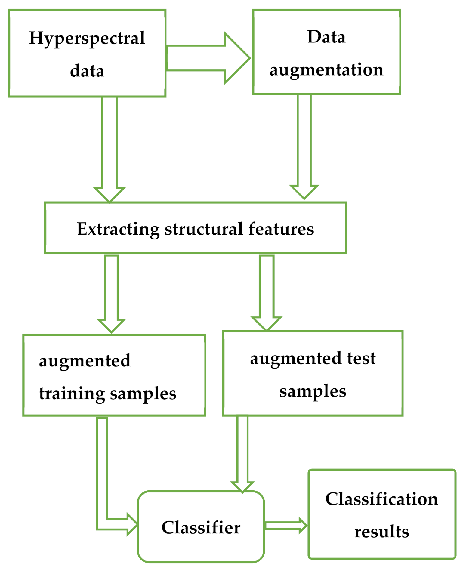
The general flow chart is shown in
Figure 1.
2. The Proposed Data Augmentation
Data augmentation is an effective method of solving the problem of small samples. However, unlike image and text data, people’s cognition of HS data is not perfect, and the augmentation methods for image and text data are unsuitable for HS data. We hope that the added samples conform to the distribution model of the sample set, so the simple random disturbance and the augmented samples obtained by adding noise have little significance for classification.
HSIs are often obtained from earth observation, and the distribution of ground objects has certain distribution rules. Our method is described as follows. For the current samples, we search for similar samples in the neighborhood of different window sizes to generate similar sample sets of different window sizes. The cluster center of the sample set moves to the real cluster center as the scale of the sample set increases. These clustering centers are in accordance with the distribution of the sample set, so we take different clustering centers as the augmented samples of each current sample.
2.1. Data Augmentation Based on Searching Similar Samples of Different Window Sizes
HSI is a natural image with certain distribution characteristics and has the aggregation distribution characteristics of a natural image. The neighborhood of each sample always has similar samples. The key to determining the quality of new samples is to accurately search the same sample set under different window sizes. In natural images, the same kind of samples may gather together in any region shape and may be adjacent to any kind of samples. Thus, determining whether the samples are of the same kind with a fixed threshold is impossible.
We use double conditions to search similar samples, that is, we select similar samples from quantity and similarity. In the neighborhood of rule samples, we first select the most likely samples. Then, according to the similarity between the candidate and current samples, the contribution weight of the sample to the cluster center is calculated. The samples with a large similarity have a greater contribution to the cluster center than those with small similarity.
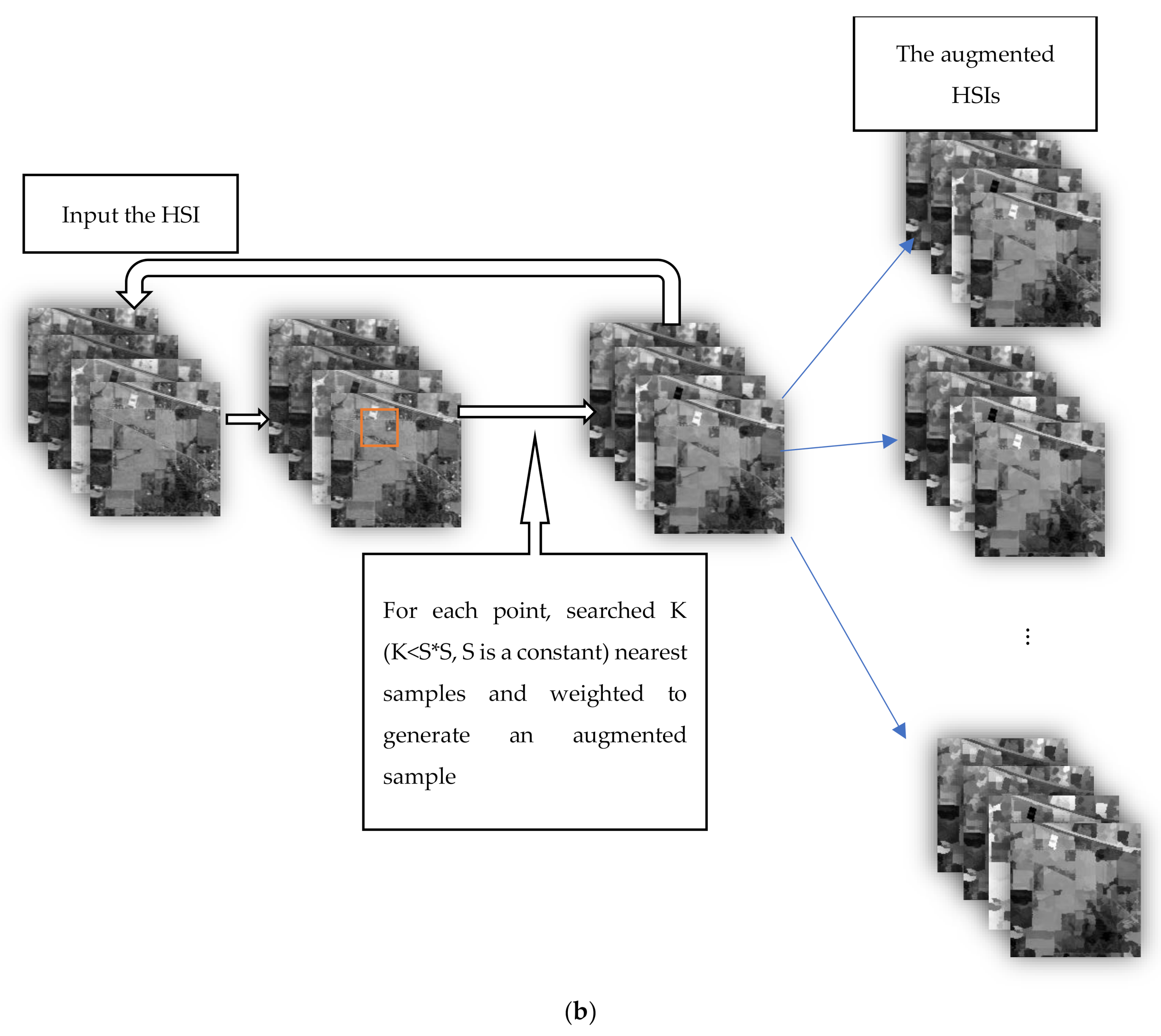
According to the above principles, we design two data augmentation algorithms. The flow chart of the two data augmentation algorithms is shown in
Figure 2.
Figure 2a is the flow chart of the data augmentation algorithm 1;
Figure 2b is the flow chart of the data augmentation algorithm 2.
2.1.1. Data Augmentation Algorithm 1
Data augmentation algorithm 1 is as follows:
1. In the HSI, the current sample is the center point, and the neighborhood regions of different window sizes are defined. The size of the region is
2. In the neighborhood region, the Euclidean distance between the neighborhood and current samples is calculated, and the samples in the neighborhood are sorted according to the distance. We select the nearest neighbor K () samples as candidate samples. The connectivity of the candidate samples is detected, and the sample points whose spatial positions are not adjacent are eliminated.
3. The contribution of the candidate sample to the augmentation sample is defined as weight. Weight
is calculated using Equation (1). Weight
is set for each candidate sample based on the similarity between each candidate sample and the current sample. If the similarity is large, then the weight is small. In Equation (1),
is the candidate sample, and
is the current sample.
4. An augmentation sample is calculated using Equation (2), where
is the augmentation sample of the current point.
5. Different-sized neighborhood windows are searched to obtain various candidate sample sets. Different candidate sample sets generate diverse augmentation sample sets of the current point.
6. The augmented samples of each pixel in the hyperspectral image are calculated to generate the augmented hyperspectral images.
2.1.2. Data Augmentation Algorithm 2
Data augmentation algorithm 2 is as follows:
1. In the HSI (after iteration, the HSI is replaced by the HSI augmentation data), the current sample is the center point. The size of window W is constant, that is,
2. In the neighborhood region, the Euclidean distance between the neighborhood and current samples is calculated, and the samples in the neighborhood are sorted according to the distance. We select the nearest neighbor K () samples as candidate samples. The connectivity of the candidate samples is detected, and the sample points whose spatial positions are not adjacent are eliminated.
3. The contribution of the candidate sample to the augmentation sample is defined as weight . Weight is calculated using Equation (1). Weight is set for each candidate sample based on the similarity between each candidate sample and the current sample. If the similarity is large, then the weight is small. In Equation (1), is the candidate sample, and is the current sample.
4. An augmentation sample is calculated using Equation (2), where is the augmentation sample of the current point.
5. The augmented sample of each pixel in the hyperspectral image are calculated to generate the augmented hyperspectral image. Return to 1, the true hyperspectral image is replaced by the augmented hyperspectral image.
6. Every iteration, an augmented hyperspectral image generates. Assuming N iterations, N augmented hyperspectral images generate
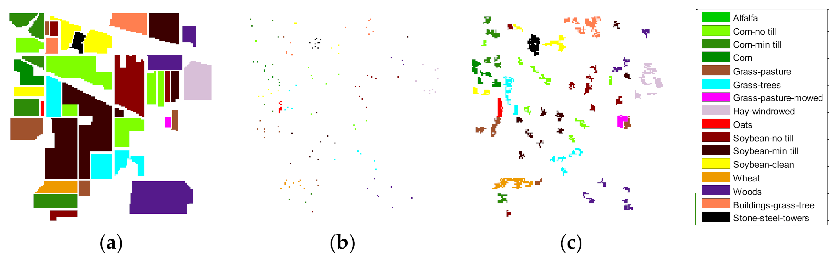
Figure 3c shows that by selecting a limited quantity of candidate samples, the same class of samples can be selected from any shape area. The fewer the number of candidate samples that are selected, the purer is the sample set of the same selected class selected. However, if the quantity is extremely small, the quality of the augmented samples will be affected.
Figure 4 presents the Indian Pines data,
Figure 4a is the training samples graph composed of 80 true training samples (16 classes, 5 training samples of each class), and
Figure 4b has 3 times the number of augmented training samples.
2.2. Optimal Selection of Test Samples after Data Augmentation
Our data augmentation algorithm not only increases the training samples, but also generates new test samples. With the expansion of the region or the increase of the number of iterations, the new augmented samples tend to move to the cluster center, that is, gradually near the real cluster center of the sample set, and the samples near the cluster center tend to have higher classification accuracy.
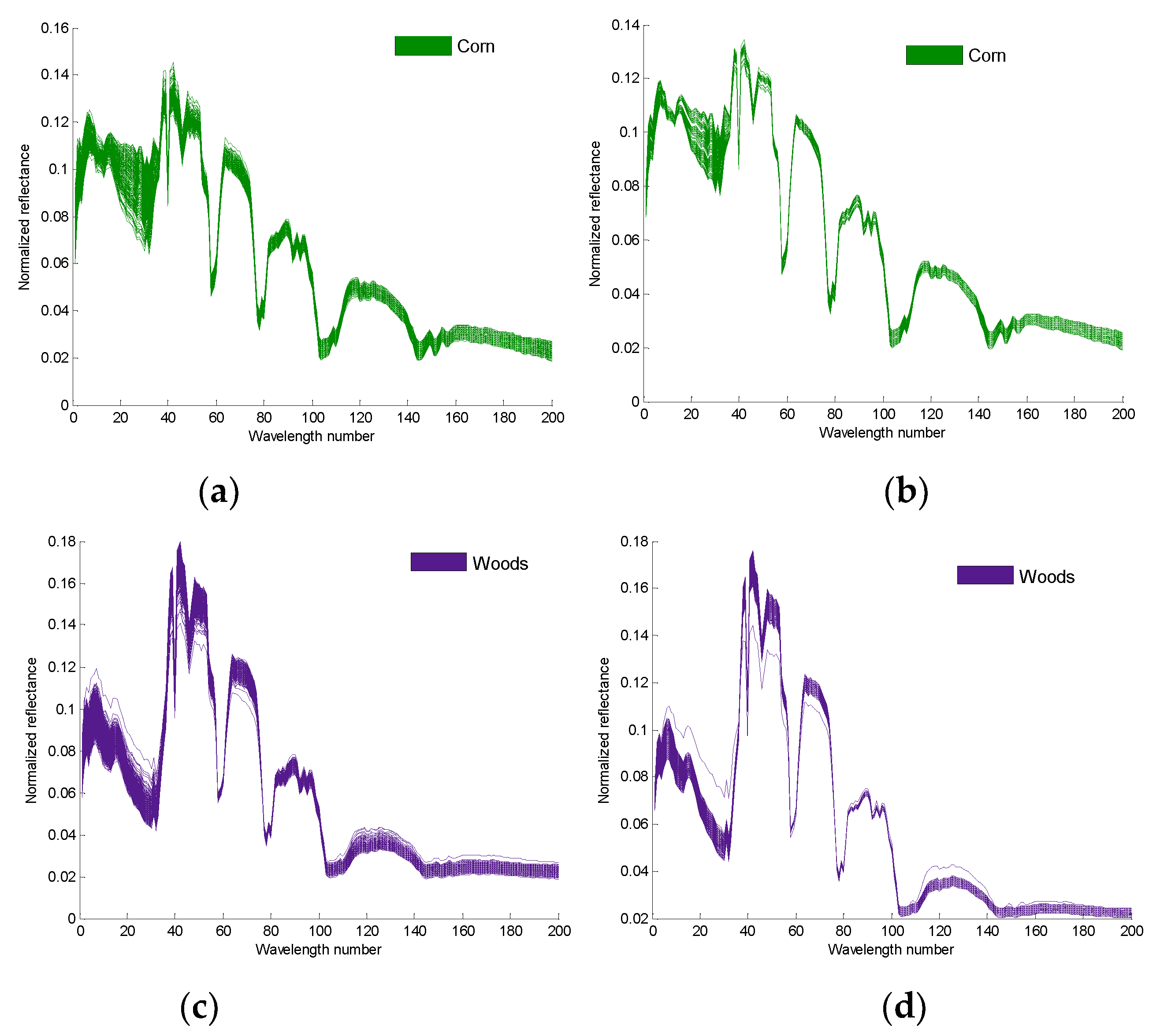
For comparison, we draw the true and augmented samples on the same figure.
Figure 4 shows that the clustering degree of the new samples is better than that of the true test sample.
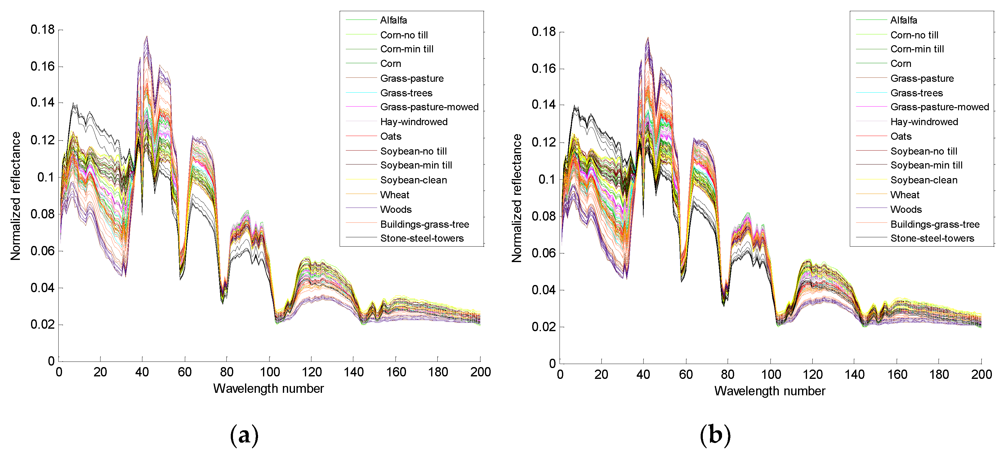
Figure 5a,c are the 4th and the 14th true spectral reflectance of the Indian Pines data, respectively;
Figure 5b,d are the augmented spectral reflectance of the Indian Pines data by the third iteration of algorithm 2, respectively.
In the fifth part of the experimental analysis, with the same classifier, the classification accuracy of the augmented test samples is significantly higher than that of the true HS test samples.
3. The Proposed Structural Feature Extraction
Structural features have many applications in the field of recognition. In image classification, handwritten numeral classification, and other fields, structural features are very important features. The deep learning developed in recent years also finds structural features conducive to classification at different scales. In the field of HS, some low-level structural feature extraction appeared in the early stage, such as the differential structure of the spectrum and structural feature extraction based on continuous wavelets [
26], which prove the effectiveness of structural features.
PCANet is a concise deep learning method that generates convolution kernels to extract structural features from different layers. PCANet extracts the last layer of features for classification. However, we think that the features that are beneficial to classification may be the structural features from different scales. We improved PCANet and designed an effective structural feature extraction method, which we call the multi structure feature fusion (MSFF) method. The flow chart of the structure extraction is shown in
Figure 6.
Our structural feature extraction algorithm is as follows:
1. Input the training samples. Calculate the mean value of each class of training samples to obtain the mean spectrum set of all classes, , denotes the class; denotes the mean sample set of the classes), and the size of the mean sample of each class is . ( is the number of bands in the mean sample)
2. For a given
,
denote a patch of
; collect all the patches (assuming size
, step is 1) around each band,
denotes a matrix of small patches,
can be expressed by Equation (3)
where each mean sample can obtain (
L −
K + 1) patches.
3. There are
N mean samples available, a total of
vectored patches are available,
denotes a matrix of patches of all classes, and
can be expressed by Equation (4)
where
is a matrix with
rows and
columns. The PCA principal components of the
matrix are calculated. Some eigenvectors with large eigenvalues are the convolution kernels of the first layer.
4. Use the convolution kernel of the first layer to extract the first volume structural features of the mean samples, and then subsample the structural features as the input of the second layer.
5. Return to the second step, and input the first volume structural features after subsampling. The size of the patch remains unchanged and the convolution kernels of the second layer are generated.
6. Use the two-layer convolution kernels to extract the structural features of the spectrum.
7.Fuse the two-tier structural features and dimension reduction into the classifier.
4. MLR /SVM Classification
To test the advantages and universality of the proposed method for classification, two classifiers: multiple linear regression (MLR) classification and support vector machines (SVM) classification are used to classify the samples processed by our method. Experiments show that MLR and SVM are superior in classification with limited samples.
4.1. The Classification of the Augmentation Hyperspectral Data (HS_AUG)
The classification steps of the HS_AUG data are as follows:
1. According to the augmentation algorithm, each pixel of the hyperspectral image can generate (assuming times of augmentation) independent augmentation samples. If the true sample is added, then each pixel has independent samples. Each of the (N + 1) samples independently represents the current pixel. If pixels are taken as the training pixels, then we will have training samples to train the classifier, and the number of training samples will be increased by times.
2. We use training samples to train the classifier.
3. The final classification decision can be realized in two methods: First, each test pixel also has independent test samples, which are sent to the classifier for independent judgment, and the current pixel prediction result is determined using the voting method. Second, the last augmented test sample of the augmentation algorithm is selected as the test sample of the current pixel (the last augmented sample is closer to the cluster center) and then sent to the above classifier for prediction.
4.2. The Classification of the Augmentation and Msff Structural Feature Hyperspectral Data (HS_AUG_MSFF)
The classification steps of the HS_AUG_MSFF data are as follows:
1. All hyperspectral data are augmented.
2. MSFF is used to extract the structural features of all data as the features of the hyperspectral data.
3. The number of training pixels is , and the number of training samples is , which are used to train the classifier.
4. The final classification decision can be realized in two methods: First, each test pixel also has independent test samples, which are sent to the classifier for independent judgment, and the current pixel prediction result is determined using the voting method. Second, the last augmented test sample of the augmentation algorithm is selected as the test sample of the current pixel (the last augmented sample is closer to the cluster center) and then sent to the above classifier for prediction.
5. Experiments and Discussion
In this section, we divide the experiment into three main parts: the data augmentation algorithm experiment, the experiment on the effectiveness of the structural features, and the comprehensive experiment on two datasets. The first two parts are the theoretical verification of the algorithm. We use MLR and SVM classifiers to verify the algorithm on the Indian Pines dataset. In the third and the fourth parts, we apply data augmentation and structural features to different data sets to calculate the classification sensitivity by MLR classification (in many experiments, the MLR classifier is better than the SVM classifier).
In the following figures and tables, each experimental data is the average of 30 experiments. All experiments are conducted in MATLAB running on an 8-GHz Intel(R) Core(TM) i5-2450M processor.
The Indian Pines and Pavia University hyperspectral data sets are adopted to demonstrate the effectiveness of the proposed method.
(1) Indian Pines dataset: This dataset is a hyperspectral image of an agricultural area collected by an airborne visible infrared imaging spectrometer (AVIRIS). The image size is 145 × 145 pixels and the spatial resolution is 20 m. It contains 220 bands (wavelength range of 0.4–2.5 m), in which 20 bands with severe water absorption are removed and 200-band hyperspectral data are retained. The data has a corresponding markup template. The dataset contains 10,366 samples with 16 known features. The high similarity of the feature spectra of the dataset and the uneven number of various sample types pose a great challenge for the high-precision classification of objects. Accordingly, this high similarity problem has been widely used in the performance testing of hyperspectral image classification algorithms.
(2) The Pavia University data set was acquired by the Reflective Optics System Imaging Spectrometer sensor during a flight campaign over Pavia, northern Italy. This data set consists of 610 × 340 pixels, with a spatial resolution of 1.3 m per pixel. After 12 noisy spectral bands are removed, 103 spectral bands are retained in the experiments. The ground truth contains nine representative urban classes.
5.1. Data Augmentation Experiment
In this part of the experiment, we verify two problems: the effectiveness of the augmented training samples and the optimal use of the augmented data.
5.1.1. Effectiveness of Augmentation
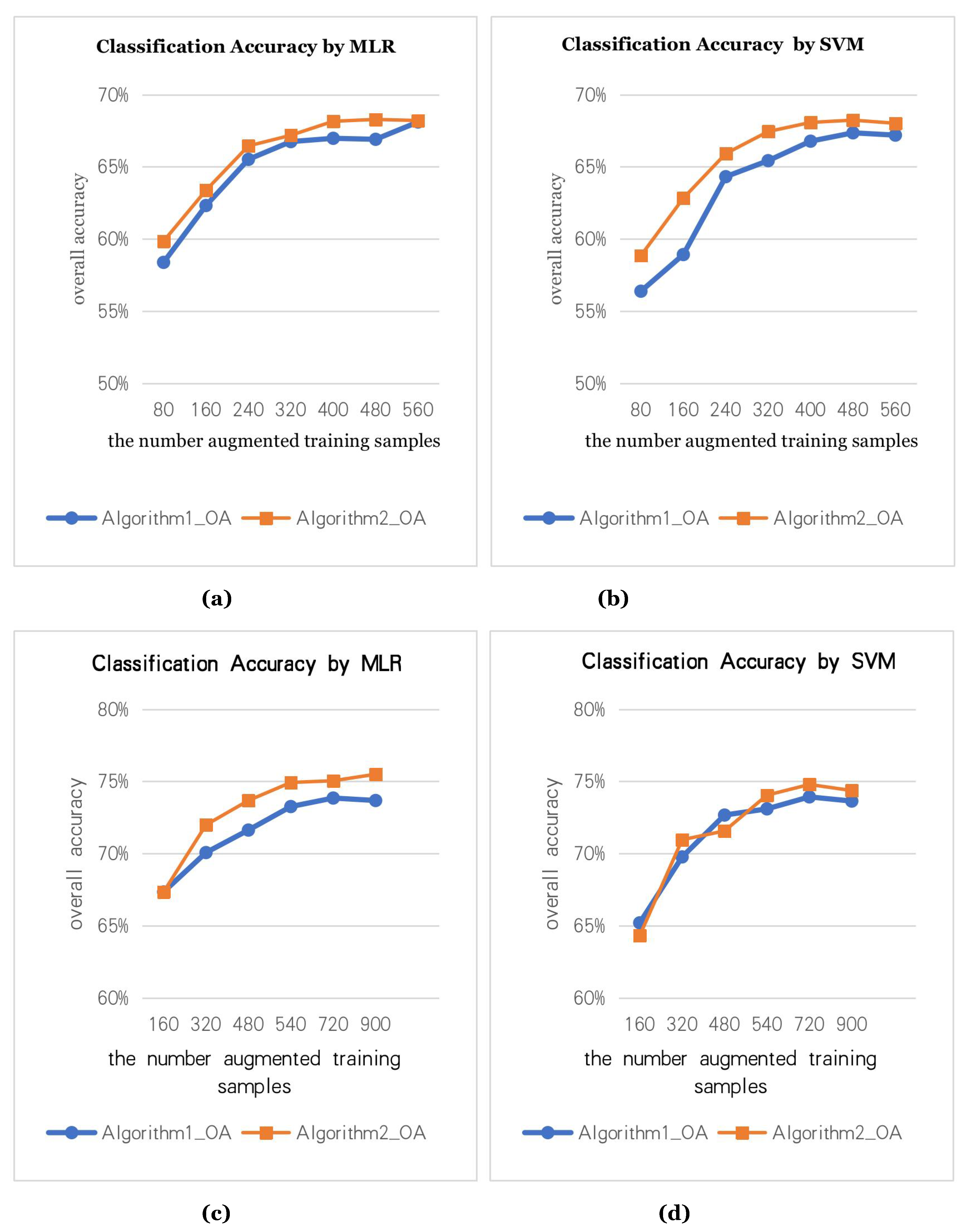
We use the data augmentation algorithm to generate the augmented training samples and calculate the classification accuracy. In the true HS data, we select different numbers of true training samples, namely, 80 true training samples (5 for each class), 160 true training samples (10 for each class).
Figure 7a,b are the classification accuracy graphs with 80 true training samples (5 for each class).
Figure 7c,d are the classification accuracy graphs with 160 true training samples (10 for each class). Two data augmentation methods are used to augment the training samples to N times, where the X-axis is the number of the augmented samples. To test the effectiveness of the data augmentation algorithm, we use two classifiers (MLR, SVM) for the experiments.
Figure 7 shows that the augmented training samples can effectively improve the classification accuracy. However, the augmentation of samples is not endless. After 3 to 4 augmentations, the classification accuracy stops improving.
In augmentation algorithm 1, the size of the neighborhood region is (3, 5, 7, 9, 11), that is, when generating augmented samples 4 to 5 times, the classification accuracy is good.
In augmentation algorithm 2, we set the size of the neighborhood region to 7. Then, the augmented samples generated by iterating 3 to 4 times have better classification accuracy.
5.1.2. Optimal Utilization of Augmented Data
The data augmentation algorithm can generate not only augmented training samples, but also augmented test samples. In this section, we discuss how to use augmented test samples. We use the augmented training samples to train the classifier and classify the true, augmented, and selected augmented test data. The three test samples are marked as test0, test_aug, and test_aug_select, respectively. For the test_aug, each pixel will obtain multiple prediction results. Here, we use the voting method to determine the prediction results of the current pixel. For test_aug_select, the prediction result of each pixel depends on the optimal augmented data.
The number of the augmented training samples are marked as the following representative variables: number_ Aug1 and number_ Aug2 (number_ Aug1 is the number of the augmented samples by data augmentation algorithm 1; number_ Aug2 is the number of the augmented samples by data augmentation algorithm 2). number_ Aug1 and number_ Aug2 are 4 times the number of the true training samples.
As shown in
Figure 8, by using the same augmented training samples to train the classifiers, different test samples will produce different classification results. The classification accuracy of the augmented test samples is higher than that of the true test samples. The classification accuracy of the selected augmented test sample is the best.
5.2. Comparison of Classification Effects of Structure Characteristics at Different Scales
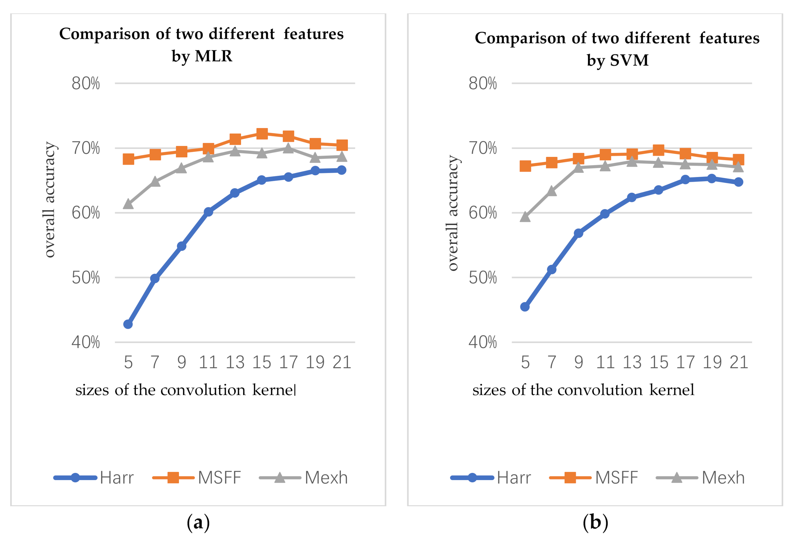
In the first part, the types of convolution kernels include Mexh wavelet, Haar wavelet, and the MSFF proposed in this work, and the scale of each convolution kernel is 5, 7, 9, 11, 13, 15, 17, 19, and 21, respectively. Mexh-OA represents the OA of the Mexh wavelet structural features. Haar-OA represents the OA of the Haar wavelet structural features. MSFF-OA represents the OA of the MSFF structural features spectrum. The number of the training for three structural features is same (10 per class).
Figure 9 presents the relationship between the classification accuracy and scales of the convolution kernels. By classifying the experiments according to the same conditions, the OA of the MSFF structural features are approximately 2% to 3% higher than that of Mexh wavelet structural features.
5.3. Comprehensive Experiment
In this section, we combine data augmentation and structural features to classify on two datasets (Indian Pines and paviaU). Given that the classification performance of the MLR classifier is better than that of the SVM, we only use the MLR classifier to perform classification experiments, calculate the classification sensitivity of the data, and draw the prediction image.
With the same number of true training samples, the classification results of the four kinds of data are compared: the true HS data; MSFF data; augmented HS data, comprehensive data augmentation and MSFF structural features data.
Table 1 shows the classification sensitivity of Indian Pines data, with 10 true training samples selected for each class.
Table 2 shows the classification sensitivity of paviaU, with 10 true training samples selected for each class.
Figure 10 and
Figure 11 are the classified prediction images.
5.4. Comparative Experiments with Other Algorithms
We compare the proposed methods (HS_AUG/HS_AUG_MSFF) with several methods, such as hyperspectral image classification using joint sparse model and discontinuity preserving relaxation (JSPR) [
42], a new deep learning-based hyperspectral image classification method RVCANET) [
41], spectral and spatial classification of hyperspectral images based on random multi-graphs (HC-RMG) [
43], and spectral–spatial hyperspectral classification via structural-kernel collaborative representation (SKCR) [
44].
The algorithms we use for comparison are comparable with the contents of this study. For example, RVCANET is a classification method based on a deep learning NN. The source codes of these methods have been provided by the true authors in literature.
During the experiment, the numbers of training samples used for all the codes are uniformly modified to 5 and 10 for each class. All methods are implemented 30 times, and their average results are calculated.
Table 3 and
Table 4 present the details of the experimental data.
Figure 12 and
Figure 13 show the results of a single experiment conducted on all the methods, using 10 training samples per class. The experiments show the superiority of the OA of the proposed method over those of existing methods with limited samples. The running time of all experiments was measured by MATLAB on an 8-GHz Intel (R) core (TM) i5-2450m processor.
6. Conclusions
Our work is divided into two aspects. First, an HS data augmentation algorithm was designed. Second, the method of extracting spectral structural features was studied.
The designed data augmentation method is different from the traditional augmentation method, which adds new samples by adding noise, rotating, and performing other operations. The method does not perform data augmentation of the image but of the spectrum. Essentially, our method uses the image attributes of the HSI to reasonably create some new samples from the neighborhood of the spectrum. The new spectrum conforms to the distribution of the spectrum, which is a meaningful data augmentation. Experiments show that when the training samples are limited, the data augmentation can effectively improve the classification accuracy. We also verified that the augmentation of unlabeled samples can greatly improve the final classification results.
Our structural feature method also proves that the structural feature of the hyperspectral data is different from the intensity feature of the spectrum, and the structural feature of hyperspectral data can even achieve better classification accuracy.
We did not use the spatial features of HSIs for classification. We only used the spatial relationship to perform spectral augmentation, and we only made some preliminary attempts on the augmentation algorithm of HS data. Thus, the method of HS data augmentation needs further development. In addition, we only designed a simple structural feature extraction method, but we look forward to better structural feature extraction methods. Effectively fusing the various structural features of the hyperspectral data will also be an important research direction.


