Article

Hyperspectral Image Classification with Localized Graph Convolutional Filtering

1
Key Laboratory of Digital Earth Science, Aerospace Information Research Institute, Chinese Academy of Sciences, Beijing 100094, China
2
Faculty of Geomatics, East China University of Technology, Nanchang 330013, China
3
School of Electronic, Electrical and Communication Engineering, University of Chinese Academy of Sciences, Beijing 100049, China
*
Author to whom correspondence should be addressed.
Remote Sens. 2021, 13(3), 526; https://doi.org/10.3390/rs13030526
Submission received: 4 January 2021 / Revised: 28 January 2021 / Accepted: 28 January 2021 / Published: 2 February 2021

Abstract

:
The nascent graph representation learning has shown superiority for resolving graph data. Compared to conventional convolutional neural networks, graph-based deep learning has the advantages of illustrating class boundaries and modeling feature relationships. Faced with hyperspectral image (HSI) classification, the priority problem might be how to convert hyperspectral data into irregular domains from regular grids. In this regard, we present a novel method that performs the localized graph convolutional filtering on HSIs based on spectral graph theory. First, we conducted principal component analysis (PCA) preprocessing to create localized hyperspectral data cubes with unsupervised feature reduction. These feature cubes combined with localized adjacent matrices were fed into the popular graph convolution network in a standard supervised learning paradigm. Finally, we succeeded in analyzing diversified land covers by considering local graph structure with graph convolutional filtering. Experiments on real hyperspectral datasets demonstrated that the presented method offers promising classification performance compared with other popular competitors.

Graphical Abstract

1. Introduction

The hundred contiguously narrow bands of hyperspectral images (HSIs) feature the hyperspectral remote sensing research fields [1]. HSIs make high-resolution spectral or spectral-spatial information extraction possible on account of their ability to carry a high volume of information [2]. Hyperspectral information extraction often involves noise estimation, endmember extraction, spectral unmixing, classification, and target detection phases based on hyperspectral data processing and analysis [3,4,5,6]. Hyperspectral remote sensing image analysis has a great power to recognize the materials of the land surface at a fine level compared to RGB (red, green, and blue) or multispectral image analysis [7,8]. However, it is unable to ignore that adjacent bands in high-dimensional hyperspectral data might be highly correlated, resulting in the Hughes phenomenon (or called the curse of dimensionality) [9], so desiring a large number of labeled samples [10,11]. And then, varying spectral signature and limited training samples at hand would probably raise the unanticipated dilemma that we have to solve the small sample classification problem [12]. When it comes to HSI classification tasks, the early-staged machine learning methods might (1) heavily rely on the handcrafted spectral-spatial features [13], (2) fail to accurately learn class conditional densities [2], (3) not accommodate limited training samples faced with the high dimensionality of hyperspectral data [6]. In the above regard, Gao et al. (2014) propose a subspace-based approach to reduce the dimensionality of the input space and facilitate the exploitation of the limited training samples [14]. Yu et al. (2016) introduced a novel supervised classifier for HSI classification combining spectral and spatial information [15]. Gao et al. (2016) combined locality-preserving projection and sparse representation to balance the high dimensionality of hyperspectral data and the limited training samples [16]. Yu et al. (2017) integrated the locality-sensitive discriminant analysis with the group sparse representation for HSI classification [17]. Gao et al. (2017) presented an optimized kernel minimum noise fraction transformation algorithm for the efficient feature extraction of HSIs [18]. Yu et al. (2017) presented a multiscale super pixel segmentation method to model the distribution of classes based on spatial information [19]. Henceforward, the deep learning technique has been increasingly favored by the scientific community attributing to its great power of abstracting representations to classify hyperspectral cubes into certain land cover categories [20,21,22,23]. As a consequence, Cui et al. (2019) proposed a multiscale spatial-spectral convolutional neural network (CNN) to integrate multiple receptive fields fused features and multiscale spatial features at different levels [24]. Gao et al. (2019) integrated t-distributed stochastic neighbor embedding with a CNN to capture the potential assembly features of HSIs [25]. Yu et al. (2020) proposed a novel method to exploit local spectral similarity and nonlocal spatial similarity by considering spatial consistency [26]. Liu et al. (2020) proposed a novel lightweight shuffled graph convolutional network (GCN) to accelerate the training procedure through a limited number of training data [27]. Making a mark on the latest, the recent novelties regarding graph representation learning have attracted more and more attention from the community.
Graph neural networks (GNNs) are a class of deep learning methods designed to perform inference on data described by graphs [28]. Deep learning as a data-driven machine learning technique has undoubtedly brought enormous prosperity in hyperspectral remote sensing intelligent information extraction depending on the high-level representational ability [29]. CNNs, as a kind of attractive representation of deep learning models, have also achieved promising results in analyzing HSIs [1]. Particularly, the CNNs’ localized kernels could efficiently recognize identical features beyond their spatial locations. Although CNN has been successful on the domains with underlying grid-like structured data, the CNN-based methods suffer from several intrinsic drawbacks summarized by the previous studies [30,31], i.e., (1) only adapting to the regular squares regardless of the geometric changes in object regions, (2) difficulty in capturing the valuable information of class boundaries during convolving a punch of patches as the convolution kernels have fixed shape, size, and weights, (3) often take a longer training time to fit huge parameters, (4) incapable of modeling topological relations among samples whether local or nonlocal feature extraction. In this regard, the graph-based convolutional neural networks appear relatively promising to overcome the aforementioned defects and show excellent characteristics, i.e., (1) competently process the irregular image regions in the non-Euclidean (or non-grid) graph data structure, (2) multiple graph inputs can be dynamically updated and refined with multiscale neighborhood [30]. It is worth mentioning that graph representation learning represented by GCNs has received increasing attention in quantifying nonlinear features in irregular graphs converted from hyperspectral data.
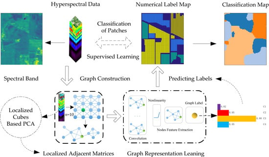
Inspired by the previous works on spectral graph-based CNN [31], its key components have been employed to adapt the HSI classification task (see Figure 1). The main contributions of this study are summarized below.
(1)
The usual supervised setting regarding fitting the graph-based learning models is designed through collecting the patch-based feature cubes and localized graph adjacent matrices.
(2)
The graph convolution layer is used to learn the spatially local graph representation and to represent the localized topological patterns of the graph nodes.
(3)
The experiments demonstrate that the presented study could achieve promising classification performance based on the localized graph convolutional filter.
The rest of this paper is organized as follows. We first reviewed the latest works relevant to HSI classification with the graph-based methods in Section 2. Then, we provide the preliminaries and definitions in Section 3. The technical details of our graph-based representation learning method are presented in Section 4. Next, we analyze the experimental results and discuss the derived findings in Section 5. Finally, the concluding remarks are given in Section 6.

2. Related Work

Graphs are a kind of universal representation of non-Euclidean structured data, which could encode complex geometric structures [32]. The following studies regarding the graph-based HSI classification approaches have gained significant attention in the last few years. Therefore, we offer a glimpse of their scientific contributions. Hyperspectral data usually reside on a nonlinear sub-manifold, causing the inefficiency of linear algorithms [1]. Manifold learning-based algorithms have been applied for the exploration of the nonlinear structure of HSI [33]. Graph-based semi-supervised learning usually constructs a graph from the labeled and unlabeled samples for manifold representation [2]. Ma et al. (2014) presented a study of the local manifold learning to preserve the local geometry of each neighborhood by finding the relationships between the nonlinear data points [34].
Sparse representation-based graph learning algorithms are good at obtaining the adjacency relationships among the samples and weights [35]. Tan et al. (2015) constructed a block sparse graph by combining sparse representation and the regularized collaborative representation for HSI classification based on discriminant analysis [36]. Luo et al. (2016) employed manifold learning based on sparse representation to illustrate the manifold structure of HSI [37]. De Morsier et al. (2016) proposed a graph representation with the kernel low-rank and sparse subspace clustering for the classification of his, assuming that hyperspectral data lies on the union of manifolds [38]. Based on the previous works, Shao et al. (2017) proposed a probabilistic class structure to estimate the probability relationship between each sample point and each class of the whole data [39]. Hong et al. (2019) proposed a graph-based semi-supervised learning method for analyzing the discriminant behavior of the labeled samples to assess the class separability [40].
As spectral information alone is not useful for discriminating different classes, the superior classification performance could be achieved through exploiting the spatial neighborhood information along with spectral information [41]. Camps-Valls et al. (2007) presented a graph-based composite kernel model for learning spectral-spatial information in a semi-supervised way [42]. Gao et al. (2014) proposed a two-layer graph-based framework to overcome the challenges of limited data and the compound distribution of classes [43]. Martínez-Usó et al. (2014) proposed a transductive approach for graph-based semi-supervised learning based on the probabilistic relaxation theory [44]. Wang et al. (2014) classified newly introduced samples by constructing the spectral–spatial graph while the unlabeled samples could be randomly selected relying on the spatial information [45]. Luo et al. (2016) proposed a graph-based model considering both spatial and spectral information [46].
The sparse representation-based graph semi-supervised learning technique combined with spectral–spatial feature learning has been proven to be effective to boost the resultant classification performance. Kruse et al. (2003) constructed a hypergraph model to explore the high-order relationships among training samples and then performed a semi-supervised hypergraph learning based on a locality constraint low-rank representation method [47]. Chen et al. (2017) conducted the double sparse graph discriminant analysis based on mining the positive and negative relationships among the data points for the dimensionality reduction in HSI in a semi-supervised manner [48]. Xue et al. (2017) adopted the sparse graph regularization for getting a more accurate classification map [49]. Aydemir and Bilgin (2017) used subtractive clustering to select training samples and extract the kernel sparse representation features to fit a support vector machine (SVM) classifier [50].
In the latest literature, GCNs have been successfully applied in irregular (or non-Euclidean) data representation learning [8]. The label information of each sample is propagated to its neighboring samples until a global stable state is reached on the complete dataset [2]. Earlier, the feature extraction and classification module has been assembled separately or executed step-by-step. As such, some scholars tried the spatial fusion technique to extract the spectral–spatial features, and then the fused features are fed into a CNN framework to learn the class distribution [12,51]. Cao et al. (2016) proposed a graph-based convolutional neural network, which used the Schroedinger Eigenmaps algorithm by incorporating a cluster potential matrix to encode spatial proximity and takes CNN as a spectral-spatial classifier to predict the accurate labels of pixels [12]. Shahraki and Prasad (2018) defined three spectral–spatial weighted affinities, (1) unsupervised adjacency matrix by using the raw reflectance spectra, (2) supervised adjacency matrix through extracting discriminative features using CNN, and (3) semi-supervised adjacency matrix via learning the limited amount of labeled samples and extensive unlabeled samples, to demonstrate the data resided on manifold structure (i.e., graph structure) [52]. Liu et al. (2020) extracted the extended morphological profiles and then conducted graph construction by the k -neighbors method, then fed into a GCN framework [20].
Recent advances in HSI classification also tended to improve the traditional GCN-based methods to inspire novelties in diverse learning paradigms [53]. As traditional GCNs might fail to utilize spectral signatures without considering spatial structures embedded in hyperspectral data, Qin et al. (2019) presented a semi-supervised spectral–spatial GCN framework and claimed that a general backpropagation rule of error could benefit the final classification performance [7]. Wan et al. (2019) made multiple graph inputs dynamically updated and refined with a novel dynamic graph convolution operation, then multiple graphs with different neighborhood scales could serve for extracting spectral–spatial features in different scales [11]. Hong et al. (2020) introduce the mini-batch strategy to improve GCN, which is capable of processing large-scale data and out-of-samples, and then jointly fused CNN (to extract the spectral–spatial features) and GCN (to analyze the relation representations) by testing three fusion schemes [10]. The deeply semi-supervised learning models have drawn more attention depending on their peculiar advantages of mining the unlabeled data to alleviate the annotating burden in the last couple of years [54].
Relevant to this study, most related works pay attention to the graph-based semi-supervised learning methods for HSI classification. The graph-based semi-supervised technique makes the input data built on the full graph, which combines the labeled and unlabeled nodes by employing a graph Laplacian regularizer when training and evaluating node classification models. The unlabeled nodes are completely observed during training or testing, whereas the standard formulation of semi-supervised learning requires the independent and identically distributed assumption between the labeled and unlabeled nodes [55]. In this case, the special concern of how to follow the usual supervised setting is raised as a research problem associated with our scientific motivation in this study.

3. Preliminaries

3.1. Graph Structure

An undirected graph is represented by G = V , E , A . V is a finite set with V = n vertices which signify both the labeled and unlabeled data samples. E is the edge set which denotes the similarities among the labeled samples as well as the unlabeled samples from the dataset. The A R n × n is a weighted adjacency matrix (i.e., graph weights) encoding the connection weight between two vertices. Note that, given a signal x defined on the nodes of the graph, which can be regarded as a vector x R n , x i is the value of x at the i t h node.

3.2. Adjacency Matrix

The graph adjacency matrix is usually calculated by measuring the similarity between two spatial neighborhoods. The adjacency matrix can be denoted as A = a i j R n × n , which defines the relationships (or edges) between vertexes. Each element a i j A can be generally computed by using the following:
(1)
the radial basis function a i , j = exp x i x j 2 σ 2 [8] or the Gaussian similarity function a i , j = exp x i x j 2 2 σ 2 [2], where σ is a parameter to control the width of the neighborhoods, the vectors x i and x j denote the spectral signatures associated to the vertexes v i and v j , respectively;
(2)
the distance function a i j = x p = c = 1 C x i c x j c p 1 p ,   p 1 is defined between two samples x i and x j , where p is an optional parameter, and C is the dimension of the feature vector. When p is 1 or 2, it becomes Manhattan distance or Euclidean distance (i.e., used in this study), respectively. The distance metric of all sample pairs can form a symmetric distance matrix A m = a i j R n × n . For example, a i j at row i and column j in the matrix A m denotes the distance between the i t h pixel and the j t h pixel [20].

3.3. Graph Laplacian

Once A is given, the corresponding graph Laplacian matrix L can be defined as L = D A , where D = d i a g d 1 , d 2 , , d N is a diagonal matrix representing the degrees of A , and d i = j a i j is the degree of the node i . To enhance the generalization ability of the graph, the symmetric normalized Laplacian matrix L ^ can be given as L ^ = D 1 2 L D 1 2 = I D 1 2 A D 1 2 , where I is an identity matrix [32].

3.4. Graph Fourier Transform

As L is a real symmetric positive semidefinite matrix, it has a complete set of orthonormal eigenvectors u i R n known as the graph Fourier modes [31]. The associated ordered real nonnegative eigenvalues λ i R n of the set of eigenvectors can be identified as the frequencies of the graph. The Laplacian is further diagonalized by the Fourier basis U = u i R n × n , such that we could perform spectral decomposition on L . So, we could have L = U Λ U 1 , where U = u 1 , u 2 , , u n is the set of eigenvectors of L and Λ = diag ( [ λ 1 , , λ n ] ) R n × n . As U is the orthogonal matrix, i.e., U U T = E , the L can be written as L = U Λ U 1 = U Λ U T . In this regard, there is a signal x R n , its graph Fourier transform can be defined as x ^ = U T x R n , and its inverse is x = U x ^ [56]. Furthermore, the given basis functions of F can be equivalently represented by a set of eigenvectors of L [8]. Therefore, the F of f on a graph can be expressed as G F f   =   U T f , and the inverse transform becomes f = U G F f , G ( F [ ] ) or G ( [ ] ) denotes an operator on the graph in the Fourier domain.

4. Proposed Method

4.1. Graph Construction

Whether the graph-based quasi-semi-supervised learning in the literature or the usual supervised learning in this study, both require the construction of graph data from the labeled and unlabeled samples using a graph Laplacian regularizer to smooth the classification function for the data manifold [2]. Accordingly, the high-dimensional hyperspectral data could be transferred into a low-dimensional subspace adapting to low-dimensional modeling and computation. Here, a graph was constructed with nodes and edges, where the nodes were specified by the unlabeled and labeled samples, whereas the edges specified the similarities among the labeled as well as the unlabeled samples. The effect of the Laplacian regularizer depends upon the construction of the graph adjacency matrix. As illustrated in Figure 2, the construction of the graph structure involved (1) the determination of localized graph adjacency relationships and (2) the calculation of multiple graph weights that have the number of samples. Finally, the correct label of land cover classes could be assigned to each patch-based hyperspectral cube after fitting the deep graph representation model in a standard supervised learning paradigm.
The high-dimensional data distribution might form an overlap of multiple manifolds [2]. The existing methods assume that hyperspectral data are a single manifold (follows label smoothness assumption) or multiple well-separated manifolds (i.e., dissatisfy label smoothness assumption). A graph can be constructed with k -nearest neighbor ( k -NN) edges. The nearby nodes are strongly connected and have similar labels. Therefore, the original hyperspectral data are spectral vectors structured in regular grids requiring to be converted into graphs in the irregular (or non-Euclidean) domain before deeply learning graph representations, given hyperspectral data matrix X R n × c , where n is the number of samples, and c (e.g., 10) is the feature dimension. Because hyperspectral data contain redundant information of a huge volume, feature reduction is one of the widely used techniques in machine learning-based HSI processing [40,48]. In terms of deep learning methods represented by CNNs, the contribution of using principal component analysis (PCA) has been known to be limited. As for the presented GCN, we found the PCA transformation was workable to enhance the classification performance. In this regard, we tried the PCA preprocessing (note that the number of components was set as 10) to extract unsupervised features and reduce the effects of intrinsic data correlation and noise. Finally, the graph adjacency matrix could be constructed by the k -NN.
The k -NN based graph construction method is most favored by the remote sensing community [2]. The adjacent matrices (i.e., graph weights) of a k -NN graph are computed by selecting k -connected neighbor nodes closest to the central node x i from the given data. That is, to compute the weighted graph of k -neighbors for pixels in X R n × c , a set of localized weight matrices (i.e., adjacent matrices) A i i = n will be normally calculated among all labeled and unlabeled samples to participate in the classification procedure. So, the neighbor nodes x i and x j have an associated weight (e.g., w i j = 0 means no connection). Notice that most graph construction methods use k -NN to generate adjacent matrices (adjacent graph). Nevertheless, k -NN might fail to obtain sufficient discriminant information.

4.2. Graph Convolution Filter

There are two strategies to define convolutional filters, either from a spatial approach or from a spectral approach [31]. The convolution theorem defines convolutions as linear operators diagonalized on the Fourier basis (represented by the eigenvectors of the Laplacian operator) [57]. Given two basis functions f and g , then their convolution can be written as f ( t ) g ( t ) = f ( τ ) g ( t τ ) d τ , where t is an independent variable, τ is the shifting distance, and denotes the convolution operator (or using G or G ( ) denotes a convolution operator on the graph). Through the well-known theorems presented in [58], the convolution can be generalized to f g = F 1 { F [ f ] × F [ g ] } , where × is the element-wise Hadamard product, and F 1 denotes an inverse Fourier transform. Hence, the convolution operation on a graph can be converted to define the Fourier transform F or find a set of basis functions. According to the graph Fourier transform addressed before, the convolution between f and g on a graph can be further expressed as G [ f g ] = U U T f × U T g .

4.3. Localized Graph Convolution

When it comes to the construction of localized graph convolution operators, spatial approaches provide filter localization via setting the finite size of the kernel, and spectral approaches, such as spectral filtering, could provide a well-defined localization operator on graphs via convolutions with a Kronecker delta implemented in the spectral domain [56,59]. In this regard, spectral filtering would be an effective approach to construct a graph convolution filter. Assume that by imposing an additional spectral filter g θ on the Fourier transform of a graph, we could have G ( f g θ ) = g θ ( L ) f = g θ U Λ U T f = U g θ ( Λ ) U T f , where g θ Λ is the function of the eigenvalues Λ of L with respect to the variable θ . The parameter θ R n is a vector of Fourier coefficients. As g θ is a non-parametric filter, so g θ Λ = diag ( θ ) . And then, we find that U T g could be equivalently written as g θ Λ or g θ . That is, the convolution on a graph can be formulated as G f g θ = U g θ U T f .
The non-parametric filters might have an intrinsic deficiency to be localized in node space and have a higher learning complexity [31]. In this case, the polynomial filters are introduced to parameterize the localized filters and defined as g θ ( Λ ) = k = 0 K 1 θ k Λ k , where the parameter θ = θ i R K is a vector of polynomial coefficients. The value at the vertex j of the filter g θ centered at the vertex i is given by g θ L δ j j = g θ L i , j = k θ k L k i , j , where the kernel is localized via the convolution with a Kronecker delta function δ i R n . The K relates to the minimum number of edges connecting two vertices on the graph (i.e., the shortest path distance). As a result, spectral filters represented by k t h order polynomials of the Laplacian are exactly K -localized enclosing K parameters.
When the graph convolution filter is localized with respect to K , the cost to filter a graph signal might be relatively high because of the multiplication with the Fourier basis U . A practical solution is to parameterize g θ ( L ) as polynomial functions [31], e.g., the k t h order truncated expansion of Chebyshev polynomials [60] and Lanczos algorithm [61], which can be computed recursively from L . Therefore, the localized graph convolution filter can be parameterized as the truncated expansion of the Chebyshev polynomial G f g θ k = 0 K 1 θ k T k ( L ˜ ) f and g θ ( Λ ) = k = 0 K 1 θ k T k ( Λ ˜ ) , where θ R K is a vector of the Chebyshev coefficients [4]. The T k ( L ˜ ) R n × n and T k ( Λ ˜ ) R n × n can be evaluated at the scaled Laplacian L ˜ = 2 L ^ / λ m a x I and Λ ˜ = 2 Λ ^ / λ m a x I , respectively. L ^ and Λ ^ denote the normalized L and Λ , respectively. The λ m a x denotes the largest eigenvalue of L ˜ .

4.4. Graph-Based CNN

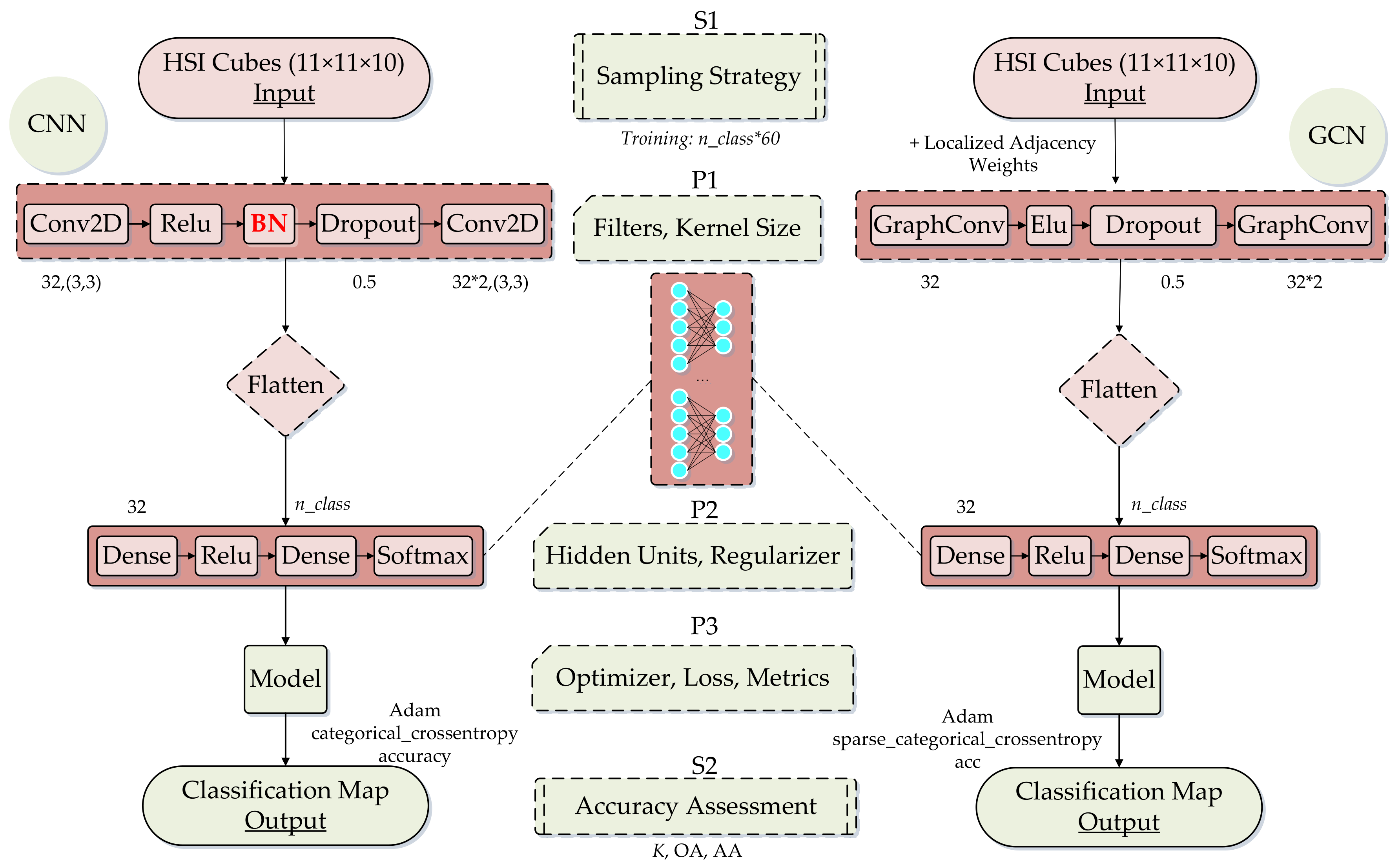
Regarding the architecture of the graph-based CNN (see Figure 3), we have the following propagation rule for fitting a designed GCN H l + 1 = h D ˜ 1 2 A ˜ D ˜ 1 2 H l W l + b l [8], where A ˜ = A + I and D ˜ i , i = j A ˜ i , j are defined as the renormalization terms of A and D , respectively. Moreover, H l denotes the output in the l t h layer and h is the activation function (e.g., ELU in this study) with respect to the weights W l l = 1 p and the biases b l l = 1 p of all layers l = 1 , 2 , , p . Particularly, the computational efficiency of the presented method is further improved using the Chebyshev approximation addressed by Rhee et al. (2017) [62].
Moreover, the l t h output feature map of the sample s is given by y s , l =   i = 1 F i n g θ i , l L x s , i R n , where x s , i are the input feature maps, and the F i n × F o u t vectors of Chebyshev coefficients θ i , l R K are the layer’s trainable parameters [31]. When training multiple convolutional layers with the backpropagation algorithm, every one of them needs the two gradients E θ i , j = s = 1 S x ¯ s , i , 0 , , x ¯ s , i , K 1 T E y s , j and E x s , i = j = 1 F o u t g θ i , j ( L ) E y s , j , where E is the loss of energy over a mini-batch of S samples. Each of the above three computations boils down to K sparse matrix–vector multiplications and one dense matrix–vector multiplication. At the top of the graph neural networks, the objective function will be formulated to minimize the training loss and to ensure robustness in terms of convergence. Finally, the unlabeled samples could be classified into different known land cover categories.

5. Experiments and Analysis

5.1. Datasets and Settings

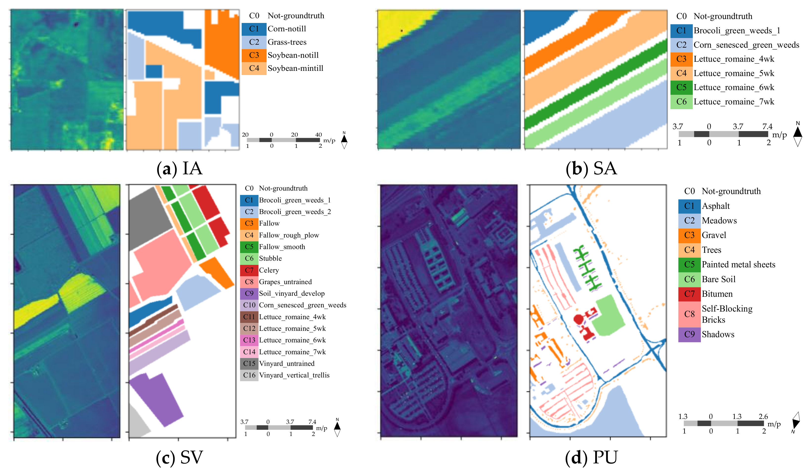
Four real hyperspectral datasets (see Figure 4 and Table 1) with different spatial resolutions were used for the experiments. The Indian Pines-A (IA), Salinas Valley-A (SA), Salinas Valley (SV), and Pavia University (PU) datasets are openly accessible online (http://www.ehu.eus/ccwintco/index.php?title=Hyperspectral_Remote_Sensing_Scenes).
The Indian Pines (IP) scene was gathered by the 224-band AVIRIS sensor in the wavelength range 400 to 2500 nm at a 20-m spatial resolution (i.e., 20 meters/pixel, or abbreviated as 20 m/p), in north-western Indiana. The IA dataset was a subset of the IP dataset, which consisted of 86 × 69 pixels and contained 200 spectral reflectance bands by removing bands covering the region of water absorption. The SV scene was also collected by the AVIRIS sensor (of which discarded 20 water absorption bands) over Salinas Valley, which comprised 512 × 217 pixels and had 16 classes, but a 3.7 m/p spatial resolution. Similarly, the SA scene was a small sub-scene of the SV scene, which comprised 86×83 pixels and had 6 classes. The PU scene was acquired by the ROSIS sensor over Pavia University, northern Italy. The PU dataset consisted of 103 spectral bands after the 13 noisiest bands were discarded, which had a size of 610 × 340 at a 1.3 m/p spatial resolution. Meanwhile, there were 9 classes included in the ground truth map.
It is of importance to select qualified training samples for fitting and evaluating the presented algorithm [63]. As listed in Table 1, the unlabeled training samples were coded as class C0 with the white background color. As for all the datasets, the size of the training set of all classes was set to 60, the same as the size of the validation set (i.e., n c l a s s × 60 ). Except for the samples included in the training and validation sets, all other samples were taken as the test set. The type of dataset might be a non-negligible factor in this study. The PU dataset was collected over an urban area. The IA, SA, and SV datasets were collected in a natural area. The IA and SA scenes belonged to simple datasets with low data complexity, while the SV and PU scenes appeared relatively complex, whether in spatial scale or landscape diversity. Moreover, the IA and SA datasets had a large proportion of ground truth samples relative to the entire scene and the lower intra-class variability. These intrinsic differences were crucial for investigating the representation ability of deep learning models on simple or complex data.
The experimental platform was a laptop equipped with an Intel Core i7-9750 12-core 2.60 GHz processor, a 256GB SSD, a 1T HDD, a 16 GB RAM, and an 8G GDDR6 NVIDIA RTX 2070 graphics card. The experimental procedures ran on the GPU aimed to achieve a higher computational speed. As only small training data was used, the time consumption of experiments could be controlled within a few minutes with the 5 and 10 independent runs and 200 epochs (or early stopping over 100 epochs) per run. It was relatively fast and showed promising efficiency in terms of complex networks. To ensure a complete comparison with CNN and to improve the traditional GCN, we tried to keep the parameter settings of the network structure as similar as possible. In this regard, we ran the experiments 5 and 10 times with each model for each dataset and kept the sizes of the training and validation sets independent. These sets of samples were randomly shuffled to reduce the possible influence of random effects, and the statistical accuracies were recorded.
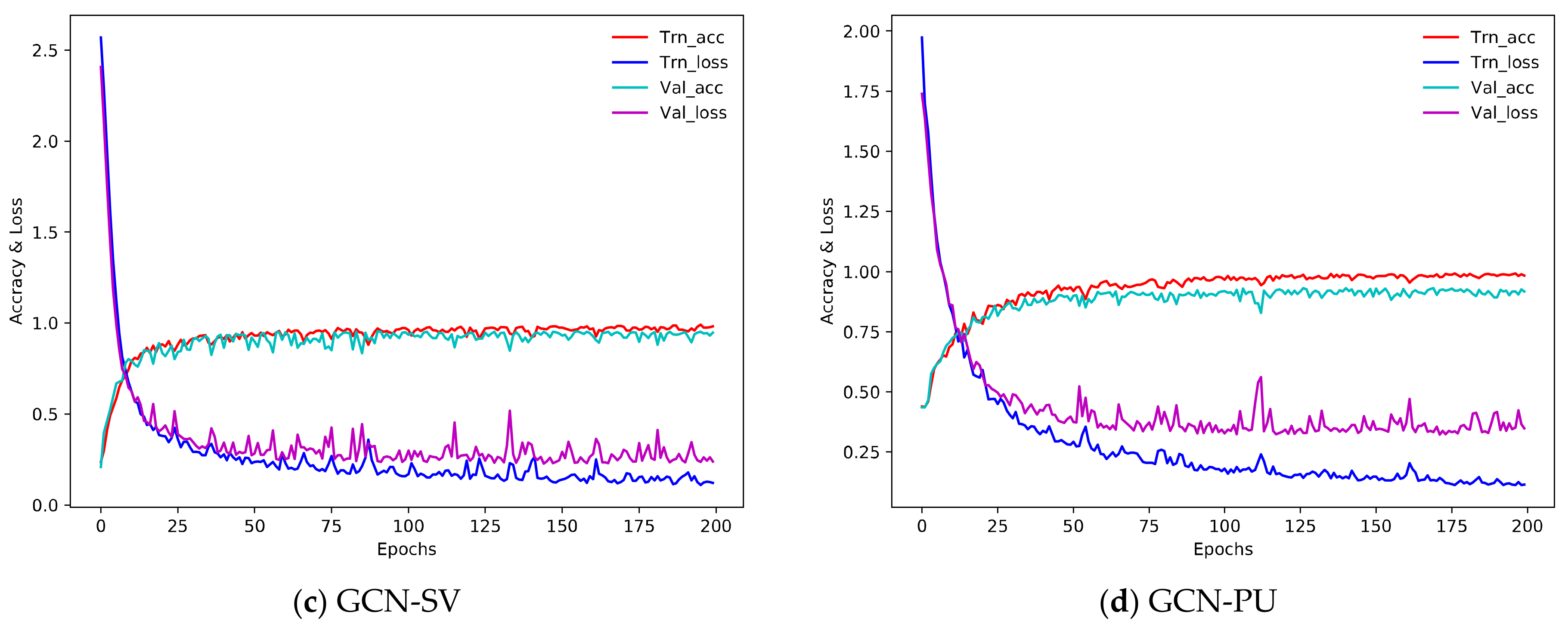
The training details incorporated the accuracy and loss of the training and validation procedures. Many factors impacted these curves, which show whether a model is qualified enough or its parameter configuration is appropriate for the subsequent parameter learning. The experiments demonstrated that, for the simple datasets, i.e., the IA and SA datasets, the CNN and GCN models appeared to converge gradually and showed good convergence behavior. When it came to the complex datasets, i.e., the SV and PU datasets, the CNN model stabilized much faster at ~10 epochs, while its validation loss curve (Val_loss) appeared to have an abnormal behavior of convergence, and the corresponding GCN model was getting better slowly (see Figure 5). As a whole, the GCN model showed a better representation of the global convergence than the CNN model, though the GCN model had some difficulties in handling the local portions, which might be influenced by the learning rate.
Relative to deep learning models, the machine learning algorithms (i.e., support vector machine (SVM)) often involve the training set (i.e., randomly selecting 60 samples of each category for fitting the classifier) and the test set, without the specialized validation set. In this study, we fine-tuned the hyperparameters (i.e., two parameters, the penalty parameter of the error term and the kernel coefficient for “rbf”). The implementation of the SVM classifier is based on “libsvm” with a one-vs.-one scheme. Moreover, all grid searches are calculated using the five-fold cross-validation. For the IA, SA, SV, and PU datasets, the best parameters obtained in the first independent run were: (1) the penalty parameter fixed at 10.0, 10.0, 100.0, and 100.0, respectively; and (2) the kernel coefficient for “rbf” determined to be 0.1, 0.1, 0.1, and 0.1, respectively. Finally, the best score was 0.8875, 0.9861, 0.9292, and 0.8481, respectively.

5.2. Classification Maps

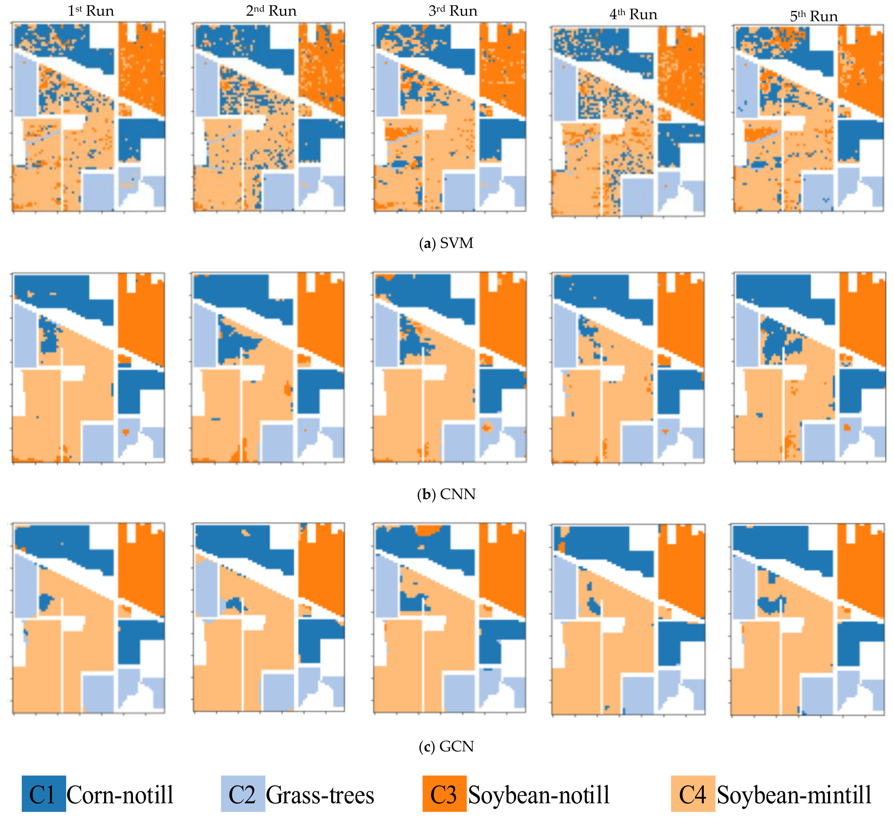
The presented experiments regarding HSI classification were achieved based on the intensity values (i.e., not the reflectance values) distributed along with spectral bands. After the training and evaluating procedures, all the unlabeled samples were classified into the proper categories; then the classification maps would be particularly helpful to assess the final classification results qualitatively. As the experiments using each algorithm for different datasets had been randomly run 5 and 10 times, we first plotted the classification maps of SVM, CNN, and the presented GCN for the IA dataset in the five running times (see Figure 6). Subsequently, the classification maps of three algorithms in the 1st run for all hyperspectral datasets were illustrated as well (see Figure 7).
As shown in Figure 6, the classification maps obtained by the SVM algorithm appeared as scattered spots, as the SVM is a pixel-level classifier essentially. The misclassifications might often be caused by the high intra-class variability and the low inter-class variability among different land cover classes. The similar results of different algorithms were commonly seen in the different random runs. The subsequent accuracy statistics and the corresponding probability maps also supported such an analysis. Referring to Figure 7, the GCN model had promising outputs compared to the other two algorithms, i.e., SVM and CNN. Furthermore, most errors of commission and omission occurred in the non-homogeneous areas involving complex landscape structures or land surface materials. The misclassifications might be mainly caused by some inherent uncertainties between classes. It is obvious that the GCN model obtained fairly good results and surpassed the SVM and CNN algorithms.

5.3. Classification Accuracies

Three widely used accuracy metrics, i.e., the Kappa index (K), overall accuracy (OA), average accuracy (AA), were used to assess the classification results, which were derived from the site-specific confusion matrix. As Table 2 illustrated, the presented GCN undoubtedly obtained the best classification performance for all the used hyperspectral datasets. Concerning the CNN model for the SA and SV datasets, the resultant accuracies appeared unanticipated. The reason is that we expanded the number of epochs from 50 to 200, and the CNN model triggered the early stopping event when monitoring its validation loss. The larger epochs might lead to a worse convergence and a decrease in performance simultaneously. Meanwhile, such a result also disclosed that the differences between the simple and complex datasets might have a significant impact on measuring performance.
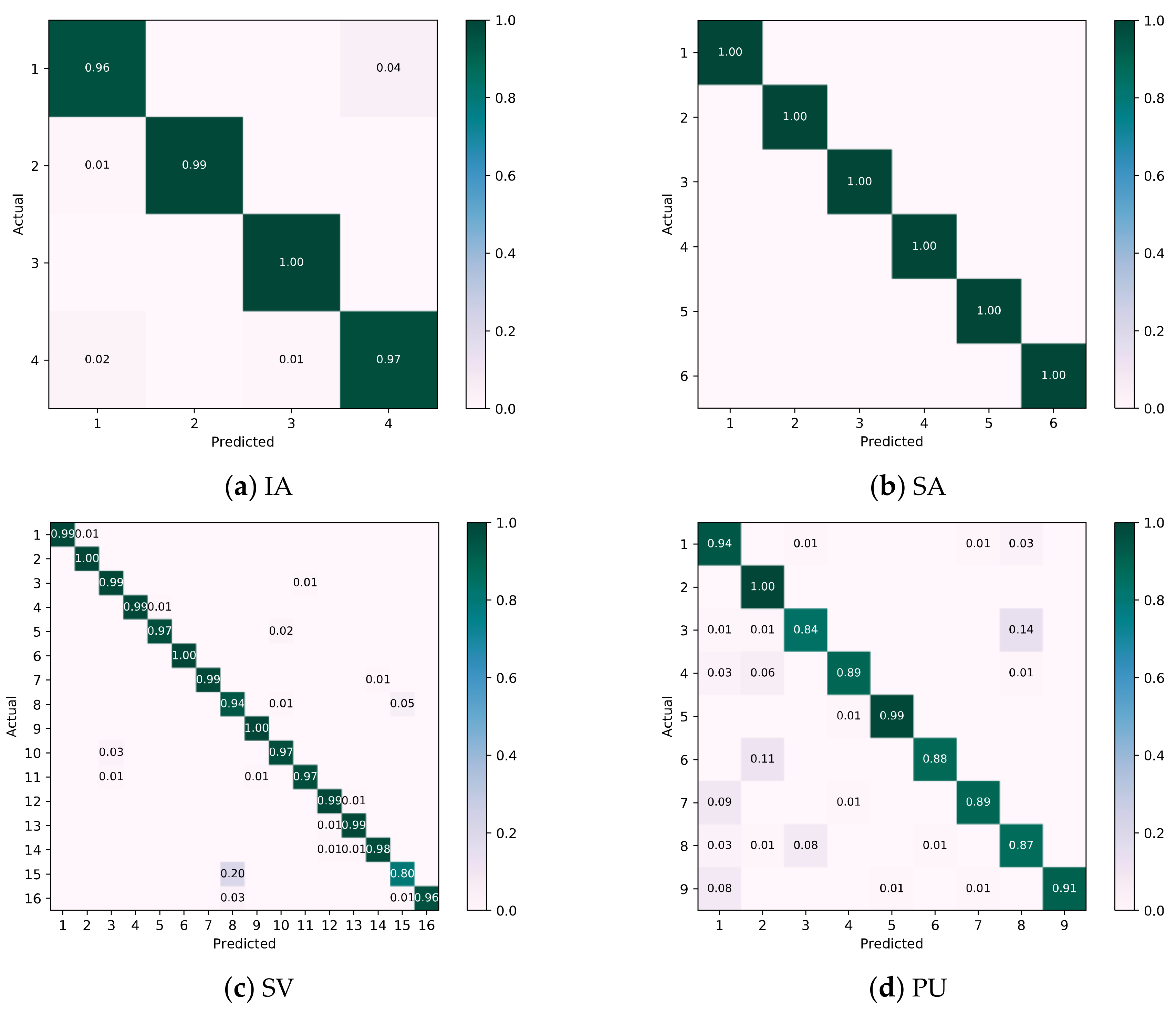
To analyze the misclassifications of the GCN model, we drew the confusion matrices for different datasets with the best performance based on the presented GCN model (see Figure 8). As for the IA dataset, we got accuracies {K: 0.9644; OA: 0.9750; AA: 0.9796}; there were 32 samples (0.04%) of Class 1 (Corn-notill) wrongly classified as Class 4 (Soybean-mintill) while there were 58 samples (0.03%) of Class 4 (Soybean-mintill) wrongly predicted as other classes, which might mean a potential inter-class negative influence. Because the SA dataset was relatively simple, the corresponding derived accuracies appeared almost saturated, i.e., {K: 0.9997; OA: 0.9998; AA: 0.9998}. For the SV dataset with accuracies {K: 0.9486; OA: 0.9539; AA: 0.9711}, most of misclassifications occurred in Class 8 (Grapes_untrained) and Class 15 (Vinyard_untrained), which might mean a conspicuous inter-class similarity between two classes. Looking at the PU dataset with accuracies {K: 0.9247; OA: 0.9436; AA: 0.9123}, more classes might get into the inter-class classification errors, probably because the PU scene was located in an urban environment and with a relatively complex landscape component.

5.4. Probability Maps

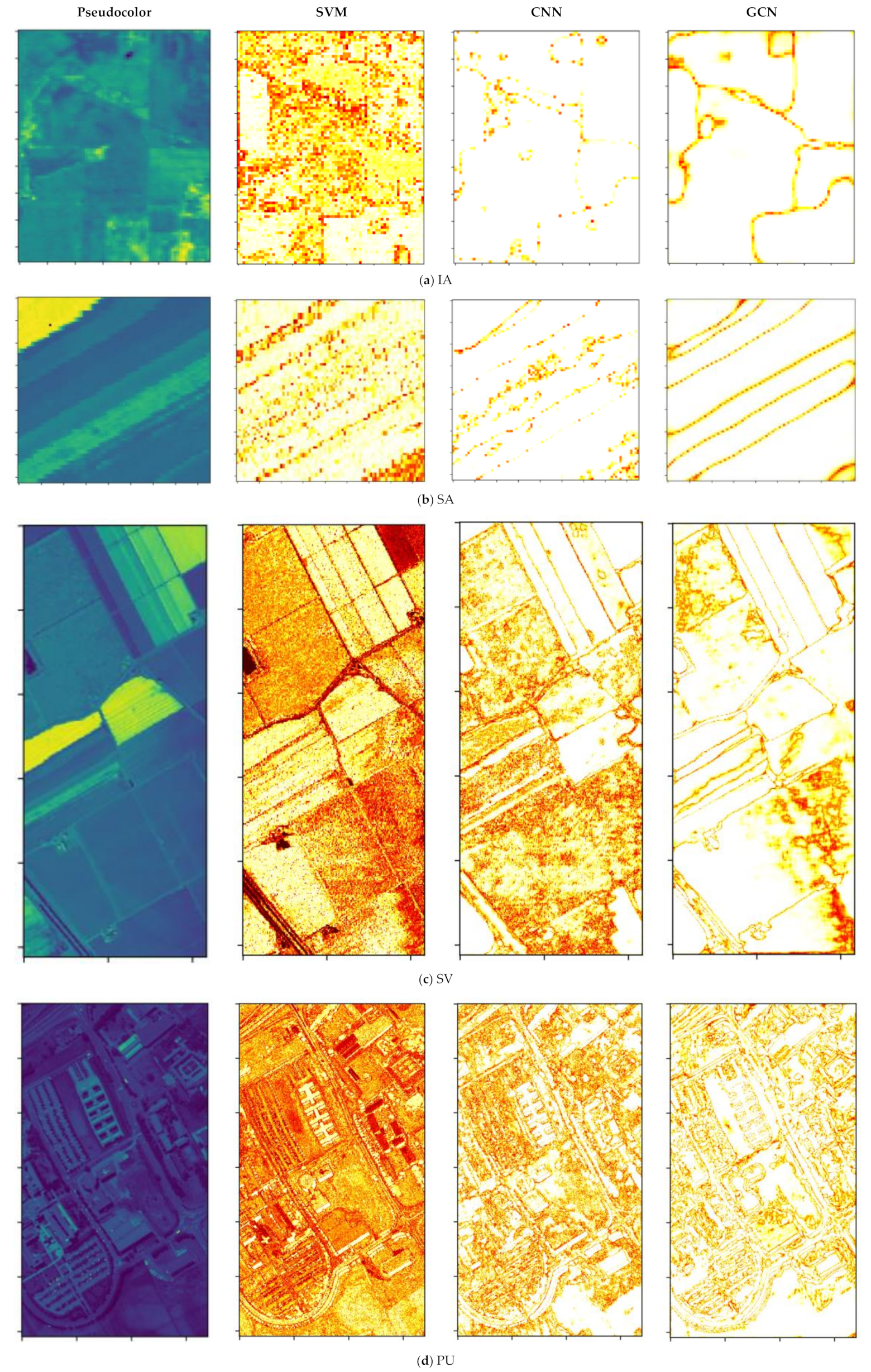
Probability density has been taken as an effective indicator to indicate the confidence of the classification output [63]. In this regard, the label assignment depends on the credible predictions with the maximum predicted probabilities and determines the final output maps. Probability maps are often utilized to observe the probability density and to find weak predictions. Therefore, we graphed the probability maps of each algorithm to show that the GCN model had clear advantages over the popular CNN model, and an apparent distinction could be reflected in the probability maps (see Figure 9).
Weak predictions in a holistic scene regarding the HSI classification task have been reported by scholars previously [63]. Figure 9 indicates the typical but not noticeable differences between the CNN and GCN models. That is, the maximum predicted probabilities of each hyperspectral cube whose central pixel was located at the edge of a category were relatively low. It seems that the GCN might be better at illustrating the boundaries among different land cover categories. Moreover, weak predictions might be more likely to occur in the cross areas and the areas covered by non-ground truth samples.

5.5. Time Consumption

The statistics of time cost are related to deep learning network structures. So, the efficiency of deep learning models can be approximately deduced as per the scales of network parameters. In practice, the training and test times are often recorded based on the clock setting of the computer operating system (see Table 3). The processing time with CPU plus GPU may depend on many possible factors, i.e., the randomness in neural networks, the efficiency of memory storage, and the difference of computational environment. Note that we tried to make the network structures of the presented CNN and GCN as comparable as possible, thus facilitating further improvement and contrastive analysis.
The differences between the presented CNN and GCN models relied on the differences between the convolution layer with a batch normalization layer and the graph convolution layer, under a comparable paradigm of network architecture design. From another perspective, both network structures had approximately the same network complexity, as we expected. Then by observing Table 3, except for the simple datasets, the presented GCN model cost ~2 times the training time than the CNN model. Such a finding could be further confirmed by the number of their network parameters (i.e., CNN: 1.22 × 10⁵; GCN: 2.50 × 10⁵).

6. Conclusions

Deep learning models have been extensively employed for HSI classification and have attracted increasing attention for their strong representation ability. Particularly, the nascent graph representation learning has shown good goodness for resolving the graph-structured data. In this study, we not only reviewed the recent publications related to the graph-based representation learning methods for HSI classification but also presented a novel graph-based spectral filtering approach that has promising benefits. It is worth mentioning that we found that the presented GCN model indeed has the advantage of illustrating the boundaries of different land cover classes by observing the weak predictions derived from the probability maps. In short, graph representation learning might represent future directions to enhance the research field of HSI classification. Future work would involve (i) testing the n-dimensional datasets where the number of components less than 10, and (ii) using the explained variance ratio for the PCA preprocessing.

Author Contributions

S.P. and Y.W. conceived and prepared the manuscript, S.P. performed the experiments and analyzed the data, and all relevant co-authors participated in writing and editing the paper. All authors have read and agreed to the published version of the manuscript.

Funding

This work was supported by the National Natural Science Foundation of China under Grant 41871245 and Grant 42030111, and funded by the Research Funding of the East China University of Technology (No. DHBK2019192).

Data Availability Statement

All data used during the study are available at http://www.ehu.eus/ccwintco/index.php/Hyperspectral_Remote_Sensing_Scenes.

Acknowledgments

The authors thank the editors and the anonymous reviewers for their insightful comments and helpful suggestions, which undoubtedly improve the quality of this manuscript.

Conflicts of Interest

The authors declare no conflict of interest.

References

  1. Rasti, B.; Hong, D.; Hang, R.; Ghamisi, P.; Kang, X.; Chanussot, J.; Benediktsson, J.A. Feature extraction for hyperspectral imagery: The evolution from shallow to deep (overview and toolbox). IEEE Geosci. Remote Sens. Mag. 2020, 8, 60–88. [Google Scholar] [CrossRef]
  2. Hong, D.; Yokoya, N.; Chanussot, J.; Zhu, X.X. An augmented linear mixing model to address spectral variability for hyperspectral unmixing. IEEE Trans. Image Process. 2019, 28, 1923–1938. [Google Scholar] [CrossRef] [PubMed] [Green Version]
  3. Gao, L.; Du, Q.; Zhang, B.; Yang, W.; Wu, Y. A comparative study on linear regression-based noise estimation for hyperspectral imagery. IEEE J. Sel. Top. Appl. Earth Obs. Remote Sens. 2013, 6, 488–498. [Google Scholar] [CrossRef] [Green Version]
  4. Zhang, B.; Sun, X.; Gao, L.; Yang, L. Endmember extraction of hyperspectral remote sensing images based on the ant colony optimization (ACO) algorithm. IEEE Trans. Geosci. Remote Sens. 2011, 49, 2635–2646. [Google Scholar] [CrossRef]
  5. Zhang, B.; Li, S.; Jia, X.; Gao, L.; Peng, M. Adaptive Markov random field approach for classification of hyperspectral imagery. IEEE Geosci. Remote Sens. Lett. 2011, 8, 973–977. [Google Scholar] [CrossRef]
  6. Zhang, B.; Yang, W.; Gao, L.; Chen, D. Real-Time target detection in hyperspectral images based on spatial-spectral information extraction. EURASIP J. Adv. Signal Process. 2012, 142. [Google Scholar] [CrossRef] [Green Version]
  7. Qin, A.; Shang, Z.; Tian, J.; Wang, Y.; Zhang, T.; Tang, Y.Y. Spectral-Spatial graph convolutional networks for semisupervised hyperspectral image classification. IEEE Geosci. Remote Sens. Lett. 2018, 16, 241–245. [Google Scholar] [CrossRef]
  8. Hong, D.; Yokoya, N.; Chanussot, J.; Zhu, X.X. Cospace: Common subspace learning from hyperspectral-multispectral correspondences. IEEE Trans. Geosci. Remote Sens. 2019, 57, 4349–4359. [Google Scholar] [CrossRef] [Green Version]
  9. Richards, J.A.; Jia, X. Remote Sensing Digital Image Analysis: An Introduction; Springer: Berlin/Heidelberg, Germany, 1999. [Google Scholar]
  10. Hong, D.; Gao, L.; Yao, J.; Zhang, B.; Plaza, A.; Chanussot, J. Graph convolutional networks for hyperspectral image classification. IEEE Trans. Geosci. Remote Sens. 2020. [Google Scholar] [CrossRef]
  11. Wan, S.; Gong, C.; Zhong, P.; Du, B.; Zhang, L.; Yang, J. Multiscale dynamic graph convolutional network for hyperspectral image classification. IEEE Trans. Geosci. Remote Sens. 2019, 58, 3162–3177. [Google Scholar] [CrossRef] [Green Version]
  12. Cao, J.; Chen, Z.; Wang, B. Graph-Based deep convolutional networks for hyperspectral image classification. In Proceedings of the 2016 IEEE International Geoscience and Remote Sensing Symposium (IGARSS), Beijing, China, 10–15 July 2016; pp. 3270–3273. [Google Scholar]
  13. Hong, D.; Wu, X.; Ghamisi, P.; Chanussot, J.; Yokoya, N.; Zhu, X.X. Invariant attribute profiles: A spatial-frequency joint feature extractor for hyperspectral image classification. IEEE Trans. Geosci. Remote Sens. 2020, 58, 3791–3808. [Google Scholar] [CrossRef] [Green Version]
  14. Gao, L.; Li, J.; Khodadadzadeh, M.; Plaza, A.; Zhang, B.; He, Z.; Yan, H. Subspace-Based support vector machines for hyperspectral image classification. IEEE Geosci. Remote Sens. Lett. 2014, 12, 349–353. [Google Scholar]
  15. Yu, H.; Gao, L.; Li, J.; Li, S.S.; Zhang, B.; Benediktsson, J.A. Spectral-Spatial hyperspectral image classification using subspace-based support vector machines and adaptive Markov random fields. Remote Sens. 2016, 8, 355. [Google Scholar] [CrossRef] [Green Version]
  16. Gao, L.; Yu, H.; Zhang, B.; Li, Q. Locality-Preserving sparse representation-based classification in hyperspectral imagery. J. Appl. Remote Sens. 2016, 10, 042004. [Google Scholar] [CrossRef]
  17. Yu, H.; Gao, L.; Li, W.; Du, Q.; Zhang, B. Locality sensitive discriminant analysis for group sparse representation-based hyperspectral imagery classification. IEEE Geosci. Remote Sens. Lett. 2017, 14, 1358–1362. [Google Scholar] [CrossRef]
  18. Gao, L.; Zhao, B.; Jia, X.; Liao, W.; Zhang, B. Optimized kernel minimum noise fraction transformation for hyperspectral image classification. Remote Sens. 2017, 9, 548. [Google Scholar] [CrossRef] [Green Version]
  19. Yu, H.; Gao, L.; Liao, W.; Zhang, B.; Pižurica, A.; Philips, W. Multiscale superpixel-level subspace-based support vector machines for hyperspectral image classification. IEEE Geosci. Remote Sens. Lett. 2017, 14, 2142–2146. [Google Scholar] [CrossRef]
  20. Liu, B.; Gao, K.; Yu, A.; Guo, W.; Wang, R.; Zuo, X. Semisupervised graph convolutional network for hyperspectral image classification. J. Appl. Remote Sens. 2020, 14, 026516. [Google Scholar] [CrossRef]
  21. Zhang, F.; Du, B.; Zhang, L. Saliency-Guided unsupervised feature learning for scene classification. IEEE Trans. Geosci. Remote Sens. 2014, 53, 2175–2184. [Google Scholar] [CrossRef]
  22. Zhong, P.; Gong, Z.; Li, S.; Schonlieb, C.-B. Learning to diversify deep belief networks for hyperspectral image classification. IEEE Trans. Geosci. Remote Sens. 2017, 55, 3516–3530. [Google Scholar] [CrossRef]
  23. Hang, R.; Liu, Q.; Hong, D.; Ghamisi, P. Cascaded recurrent neural networks for hyperspectral image classification. IEEE Trans. Geosci. Remote Sens. 2019, 57, 5384–5394. [Google Scholar] [CrossRef] [Green Version]
  24. Cui, X.; Zheng, K.; Gao, L.; Zhang, B.; Yang, D.; Ren, J. Multiscale spatial-spectral convolutional network with image-based framework for hyperspectral imagery classification. Remote Sens. 2019, 11, 2220. [Google Scholar] [CrossRef] [Green Version]
  25. Gao, L.; Gu, D.; Zhuang, L.; Ren, J.; Yang, D.; Zhang, B. Combining t-Distributed Stochastic Neighbor Embedding with Convolutional Neural Networks for Hyperspectral Image Classification. IEEE Geosci. Remote Sens. Lett. 2019, 17, 1368–1372. [Google Scholar] [CrossRef]
  26. Yu, H.; Gao, L.; Liao, W.; Zhang, B.; Zhuang, L.; Song, M.; Chanussot, J. Global spatial and local spectral similarity-based manifold learning group sparse representation for hyperspectral imagery classification. IEEE Trans. Geosci. Remote Sens. 2019, 58, 3043–3056. [Google Scholar] [CrossRef]
  27. Liu, Y.; Gao, L.; Xiao, C.; Qu, Y.; Zheng, K.; Marinoni, A. Hyperspectral Image Classification Based on a Shuffled Group Convolutional Neural Network with Transfer Learning. Remote Sens. 2020, 12, 1780. [Google Scholar] [CrossRef]
  28. Battaglia, P.W.; Hamrick, J.B.; Bapst, V.; Sanchez-Gonzalez, A.; Zambaldi, V.; Malinowski, M.; Tacchetti, A.; Raposo, D.; Santoro, A.; Faulkner, R.; et al. Relational inductive biases, deep learning, and graph networks. arXiv 2018, arXiv:1806.01261. [Google Scholar]
  29. Yang, X.; Ye, Y.; Li, X.; Lau, R.Y.K.; Zhang, X.; Huang, X. Hyperspectral image classification with deep learning models. IEEE Trans. Geosci. Remote Sens. 2018, 56, 5408–5423. [Google Scholar] [CrossRef]
  30. Wan, S.; Gong, C.; Zhong, P.; Pan, S.; Li, G.; Yang, J. Hyperspectral Image Classification with Context-Aware Dynamic Graph Convolutional Network. IEEE Trans. Geosci. Remote Sens. 2020, 59, 597–612. [Google Scholar] [CrossRef]
  31. Defferrard, M.I.; Bresson, X.; Vandergheynst, P. Convolutional neural networks on graphs with fast localized spectral filtering. Adv. Neural Inf. Process. Syst. 2016, 29, 3844–3852. [Google Scholar]
  32. Chung, F.R.K.; Graham, F.C. Spectral Graph Theory; American Mathematical Society: Providence, RI, USA, 1997. [Google Scholar]
  33. Hong, D.; Yokoya, N.; Ge, N.; Chanussot, J.; Zhu, X.X. Learnable manifold alignment (LeMA): A semi-supervised cross-modality learning framework for land cover and land use classification. ISPRS J. Photogramm. Remote Sens. 2019, 147, 193–205. [Google Scholar] [CrossRef]
  34. Ma, L.; Crawford, M.M.; Yang, X.; Guo, Y. Local-Manifold-Learning-Based graph construction for semisupervised hyperspectral image classification. IEEE Trans. Geosci. Remote Sens. 2014, 53, 2832–2844. [Google Scholar] [CrossRef]
  35. Gao, L.; Hong, D.; Yao, J.; Zhang, B.; Gamba, P.; Chanussot, J. Spectral superresolution of multispectral imagery with joint sparse and low-rank learning. IEEE Trans. Geosci. Remote Sens. 2020. [Google Scholar] [CrossRef]
  36. Tan, K.; Zhou, S.; Du, Q. Semisupervised discriminant analysis for hyperspectral imagery with block-sparse graph. IEEE Geosci. Remote Sens. Lett. 2015, 12, 1765–1769. [Google Scholar] [CrossRef]
  37. Luo, F.; Huang, H.; Ma, Z.; Liu, J. Semisupervised sparse manifold discriminative analysis for feature extraction of hyperspectral images. IEEE Trans. Geosci. Remote Sens. 2016, 54, 6197–6211. [Google Scholar] [CrossRef]
  38. De Morsier, F.; Borgeaud, M.; Gass, V.; Thiran, J.P.; Tuia, D. Kernel low-rank and sparse graph for unsupervised and semi-supervised classification of hyperspectral images. IEEE Trans. Geosci. Remote Sens. 2016, 54, 3410–3420. [Google Scholar] [CrossRef]
  39. Shao, Y.; Sang, N.; Gao, C.; Ma, L. Probabilistic class structure regularized sparse representation graph for semi-supervised hyperspectral image classification. Pattern Recognit. 2017, 63, 102–114. [Google Scholar] [CrossRef]
  40. Hong, D.; Yokoya, N.; Chanussot, J.; Xu, J.; Zhu, X.X. Learning to propagate labels on graphs: An iterative multitask regression framework for semi-supervised hyperspectral dimensionality reduction. ISPRS J. Photogramm. Remote Sens. 2019, 158, 35–49. [Google Scholar] [CrossRef]
  41. Yang, L.; Yang, S.; Jin, P.; Zhang, R. Semi-Supervised hyperspectral image classification using spatio-spectral Laplacian support vector machine. IEEE Geosci. Remote Sens. Lett. 2013, 11, 651–655. [Google Scholar] [CrossRef]
  42. Camps-Valls, G.; Marsheva, T.V.B.; Zhou, D. Semi-Supervised graph-based hyperspectral image classification. IEEE Trans. Geosci. Remote Sens. 2007, 45, 3044–3054. [Google Scholar] [CrossRef]
  43. Gao, Y.; Ji, R.; Cui, P.; Dai, Q.; Hua, G. Hyperspectral image classification through bilayer graph-based learning. IEEE Trans. Image Process. 2014, 23, 2769–2778. [Google Scholar] [CrossRef]
  44. Martínez-Usó, A.; Pla, F.; Sotoca, J.M. Modelling contextual constraints in probabilistic relaxation for multi-class semi-supervised learning. Knowl. Based Syst. 2014, 66, 82–91. [Google Scholar] [CrossRef] [Green Version]
  45. Wang, L.; Hao, S.; Wang, Q.; Wang, Y. Semi-Supervised classification for hyperspectral imagery based on spatial-spectral label propagation. ISPRS J. Photogramm. Remote Sens. 2014, 97, 123–137. [Google Scholar] [CrossRef]
  46. Luo, R.; Liao, W.; Huang, X.; Pi, Y.; Philips, W. Feature extraction of hyperspectral images with semisupervised graph learning. IEEE J. Sel. Top. Appl. Earth Obs. Remote Sens. 2016, 9, 4389–4399. [Google Scholar] [CrossRef]
  47. Kruse, F.A.; Boardman, J.W.; Huntington, J.F. Comparison of airborne hyperspectral data and EO-1 Hyperion for mineral mapping. IEEE Trans. Geosci. Remote Sens. 2003, 41, 1388–1400. [Google Scholar] [CrossRef] [Green Version]
  48. Chen, P.; Jiao, L.; Liu, F.; Zhao, J.; Zhao, Z.; Liu, S. Semi-Supervised double sparse graphs based discriminant analysis for dimensionality reduction. Pattern Recognit. 2017, 61, 361–378. [Google Scholar] [CrossRef]
  49. Xue, Z.; Du, P.; Li, J.; Su, H. Sparse graph regularization for hyperspectral remote sensing image classification. IEEE Trans. Geosci. Remote Sens. 2017, 55, 2351–2366. [Google Scholar] [CrossRef]
  50. Aydemir, M.S.; Bilgin, G. Semisupervised hyperspectral image classification using small sample sizes. IEEE Geosci. Remote Sens. Lett. 2017, 14, 621–625. [Google Scholar] [CrossRef]
  51. Ma, L.; Ma, A.; Ju, C.; Li, X. Graph-Based semi-supervised learning for spectral-spatial hyperspectral image classification. Pattern Recognit. Lett. 2016, 83, 133–142. [Google Scholar] [CrossRef]
  52. Shahraki, F.F.; Prasad, S. Graph convolutional neural networks for hyperspectral data classification. In Proceedings of the 2018 IEEE Global Conference on Signal and Information Processing (GlobalSIP), Anaheim, CA, USA, 26–28 November 2018; pp. 968–972. [Google Scholar]
  53. Hong, D.; Gao, L.; Yokoya, N.; Yao, J.; Chanussot, J.; Du, Q.; Zhang, B. More diverse means better: Multimodal deep learning meets remote-sensing imagery classification. IEEE Trans. Geosci. Remote Sens. 2020. [Google Scholar] [CrossRef]
  54. Hong, D.; Yokoya, N.; Xia, G.S.; Chanussot, J.; Zhu, X.X. X-ModalNet: A semi-supervised deep cross-modal network for classification of remote sensing data. ISPRS J. Photogramm. Remote Sens. 2020, 167, 12–23. [Google Scholar] [CrossRef]
  55. Hamilton, W.L. Graph representation learning. Synth. Lect. Artif. Intell. Mach. Learn. 2020, 14, 1–159. [Google Scholar] [CrossRef]
  56. Shuman, D.I.; Narang, S.K.; Frossard, P.; Ortega, A.; Vandergheynst, P. The emerging field of signal processing on graphs: Extending high-dimensional data analysis to networks and other irregular domains. IEEE Signal Process. Mag. 2013, 30, 83–98. [Google Scholar] [CrossRef] [Green Version]
  57. Mallat, S. A Wavelet Tour of Signal Processing; Elsevier: Amsterdam, The Netherlands, 1999. [Google Scholar]
  58. McGillem, C.D.; Cooper, G.R. Continuous and Discrete Signal and System Analysis; Oxford University Press: New York, NY, USA, 1991. [Google Scholar]
  59. Bruna, J.; Zaremba, W.; Szlam, A.; LeCun, Y. Spectral networks and locally connected networks on graphs. arXiv 2013, arXiv:1312.6203. [Google Scholar]
  60. Hammond, D.K.; Vandergheynst, P.; Gribonval, R. Wavelets on graphs via spectral graph theory. Appl. Comput. Harmon. Anal. 2011, 30, 129–150. [Google Scholar] [CrossRef] [Green Version]
  61. Susnjara, A.; Perraudin, N.; Kressner, D.; Vandergheynst, P. Accelerated filtering on graphs using Lanczos method. arXiv 2015, arXiv:1509.04537. [Google Scholar]
  62. Rhee, S.; Seo, S.; Kim, S. Hybrid approach of relation network and localized graph convolutional filtering for breast cancer subtype classification. arXiv 2017, arXiv:1711.05859. [Google Scholar]
  63. Deng, F.; Pu, S.; Chen, X.; Shi, Y.; Yuan, T.; Pu, S. Hyperspectral image classification with capsule network using limited training samples. Sensors 2018, 18, 3153. [Google Scholar] [CrossRef] [Green Version]
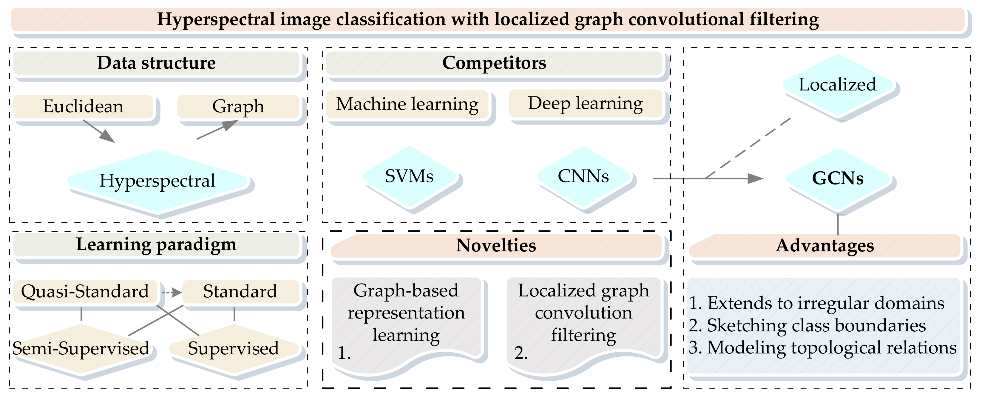
Figure 1. The overview of hyperspectral image (HSI) classification with localized graph convolutional network (GCN).
Remotesensing 13 00526 g001
Figure 2. The presented graph representation learning framework for HSI classification with the localized graph convolutional filter. Here, the localized feature cubes were created by using a principal component analysis (PCA) transformation.
Remotesensing 13 00526 g002
Figure 3. The architecture of the proposed convolutional neural network (CNN) and graph convolutional network (GCN). Here, Si {i = 1, 2} denotes the key sub-flows, and Pj {j = 1, 2, 3} represents several sets of parameter settings. Note that the CNN and GCN are completely independent networks.
Remotesensing 13 00526 g003
Figure 4. The pseudo-color images and ground truth data for four real hyperspectral datasets, i.e., (a) the IA dataset, (b) the SA dataset, (c) the SV dataset, and (d) the PU dataset.
Remotesensing 13 00526 g004
Figure 5. The accuracy & loss curves of the CNN and GCN models in the 1st run for the SV and PU datasets, i.e., (a) CNN-SV, (b) CNN-PU, (c) GCN-SV, (d) GCN-PU, corresponding to the experiment with five random runs.
Remotesensing 13 00526 g005aRemotesensing 13 00526 g005b
Figure 6. The classification maps of the presented GCN and its competitors, i.e., SVM and CNN, in five times random run for the IA dataset. The 1st, 2nd, and 3rd rows correspond to the (a) SVM, (b) CNN, and (c) GCN algorithms, respectively. Meanwhile, the 1st, 2nd, 3rd, 4th, and 5th columns correspond to different random runs, respectively.
Remotesensing 13 00526 g006
Figure 7. The classification maps of the presented GCN (the 4th column) and its competitors, i.e., SVM (the 2nd column) and CNN (the 3rd column), in the 1st run for four real hyperspectral datasets, i.e., (a) the IA dataset, (b) the SA dataset, (c) the SV dataset, (d) the PU dataset, corresponding to the experiment with five random runs.
Remotesensing 13 00526 g007
Figure 8. The confusion matrices of the presented GCN for different datasets, corresponding to the experiment with five random runs. (a) The IA dataset was at the 5th random run, (b) the SA dataset was at the 3rd random run, (c) the SV dataset was at the 3rd random run, and (d) the PU dataset was at the 2nd random run.
Remotesensing 13 00526 g008
Figure 9. The probability maps of the presented GCN and its competitors in the 1st run for four real hyperspectral datasets, i.e., (a) the IA dataset, (b) the SA dataset, (c) the SV dataset, (d) the PU dataset, corresponding to the experiment with five random runs. Note that the deeper the color, the weaker the prediction.
Remotesensing 13 00526 g009
Table 1. The division of ground truth samples for the Indian Pines-A (IA), Salinas Valley-A (SA), Salinas Valley (SV), and Pavia University (PU) datasets.
DatasetsCodesClassesTotalTrainingTestValidation
IAC0Not-ground truth1534000
C1Corn-notill10056088560
C2Grass-trees7306061060
C3Soybean-notill7416062160
C4Soybean-mintill192460180460
SAC0Not-ground truth1790000
C1Brocoli_green_weeds_13916027160
C2Corn_senesced_green_weeds134360122360
C3Lettuce_romaine_4wk6166049660
C4Lettuce_romaine_5wk152560140560
C5Lettuce_romaine_6wk6746055460
C6Lettuce_romaine_7wk7996067960
SVC0Not-ground truth56,975000
C1Brocoli_green_weeds_1200960188960
C2Brocoli_green_weeds_2372660360660
C3Fallow197660185660
C4Fallow_rough_plow139460127460
C5Fallow_smooth267860255860
C6Stubble395960383960
C7Celery357960345960
C8Grapes_untrained11,2716011,15160
C9Soil_vinyard_develop620360608360
C10Corn_senesced_green_weeds327860315860
C11Lettuce_romaine_4wk10686094860
C12Lettuce_romaine_5wk192760180760
C13Lettuce_romaine_6wk9166079660
C14Lettuce_romaine_7wk10706095060
C15Vinyard_untrained726860714860
C16Vinyard_vertical_trellis180760168760
PUC0Not-ground truth164,624000
C1Asphalt663160651160
C2Meadows18,6496018,52960
C3Gravel209960197960
C4Trees306460294460
C5Painted metal sheets134560122560
C6Bare Soil502960490960
C7Bitumen133060121060
C8Self-Blocking Bricks368260356260
C9Shadows9476082760
Table 2. The statistical classification accuracies for four real hyperspectral datasets with 5 and 10 random runs. Note that the experiments regarding a different number of random runs were carried out independently.
Alg.SVMCNNGCN
Dat./Acc.KOAAAKOAAAKOAAA
IA50.7646 ± 0.01740.8343 ± 0.01200.8574 ± 0.01360.8990 ± 0.01030.9294 ± 0.00760.9506 ± 0.00430.9550 ± 0.00640.9685 ± 0.00450.9692 ± 0.0062
SA50.9793 ± 0.00540.9836 ± 0.00430.9818 ± 0.00650.9477 ± 0.01530.9586 ± 0.01220.9701 ± 0.00790.9983 ± 0.00100.9987 ± 0.00080.9982 ± 0.0011
SV50.8370 ± 0.00760.8533 ± 0.00700.9229 ± 0.00270.7895 ± 0.01260.8101 ± 0.01150.8244 ± 0.00570.9360 ± 0.00990.9426 ± 0.00880.9614 ± 0.0090
PU50.7015 ± 0.00650.7651 ± 0.00510.8270 ± 0.00900.7238 ± 0.02350.7856 ± 0.02040.8423 ± 0.01210.9113 ± 0.00800.9336 ± 0.00590.8927 ± 0.0128
IA100.7671 ± 0.01560.8355 ± 0.01140.8613 ± 0.01060.8930 ± 0.02490.9250 ± 0.01820.9475 ± 0.00940.9579 ± 0.01040.9706 ± 0.00720.9702 ± 0.0075
SA100.9795 ± 0.00460.9837 ± 0.00360.9823 ± 0.00550.9637 ± 0.00740.9713 ± 0.00580.9783 ± 0.00380.9978 ± 0.00200.9982 ± 0.00160.9977 ± 0.0021
SV100.8389 ± 0.00800.8551 ± 0.00730.9224 ± 0.00370.7896 ± 0.00690.8105 ± 0.00640.8234 ± 0.00980.9405 ± 0.01360.9465 ± 0.01230.9663 ± 0.0063
PU100.7038 ± 0.01680.7674 ± 0.01480.8274 ± 0.00880.7218 ± 0.03140.7836 ± 0.02670.8424 ± 0.01520.9079 ± 0.01530.9309 ± 0.01170.8916 ± 0.0185
Table 3. Total network parameters and time consumption (i.e., the average time of 5 and 10 random runs). Note that the numbers in parentheses regarding datasets and models indicate the number of samples and the number of network parameters, respectively.
Alg. (Para.)/Dat. (Num.)/Time (s)IA (86 × 69 × 200)SA (83 × 86 × 204)SV (512 × 217 × 204)PU (610 × 340 × 103)
Training
(240)
Test
(3920)
Training
(360)
Test
(4628)
Training
(960)
Test
(52209)
Training
(540)
Test
(41696)
SVM51.00 ± 0.040.01 ± 0.012.22 ± 0.010.02 ± 0.0117.35 ± 0.251.29 ± 0.055.77 ± 0.010.55 ± 0.04
CNN5
(1.22 × 10⁵)
14.65 ± 4.470.31 ± 0.0117.07 ± 3.330.39 ± 0.0218.49 ± 0.275.00 ± 0.1415.03 ± 0.943.21 ± 0.05
GCN5
(2.50 × 10⁵)
13.22 ± 1.220.24 ± 0.0020.41 ± 0.720.31 ± 0.0043.39± 0.483.61 ± 0.0728.10 ± 0.593.03 ± 0.06
SVM101.05 ± 0.060.01 ± 0.002.24 ± 0.030.02 ± 0.0117.47 ± 0.201.27 ± 0.035.80 ± 0.100.56 ± 0.04
CNN10
(1.22 × 10⁵)
12.69 ± 2.980.33 ± 0.0314.79 ± 2.340.37 ± 0.0118.06 ± 1.164.79 ± 0.3113.72 ± 0.853.04 ± 0.04
GCN10
(2.50 × 10⁵)
13.50 ± 4.120.24 ± 0.0121.52 ± 1.310.32 ± 0.0150.04 ± 2.854.08 ± 0.1335.08 ± 2.693.62 ± 0.14
Publisher’s Note: MDPI stays neutral with regard to jurisdictional claims in published maps and institutional affiliations.