1. Introduction
Due to the advances in imaging spectrometry, hyperspectral sensors tend to capture the intensity of reflectance of a given scene with increasingly higher spatial and spectral resolution [
1]. The obtained hyperspectral image (HSI) contains both spatial features and a continuous diagnostic spectrum of different objects at the same time [
2]. Thus, the obtained abundant information makes HSI useful in many areas including effective measurement of agricultural performance [
3], plant diseases detection [
4], identification of minerals [
5], disease diagnosis and image-guided surgery [
6], ecosystem measurement [
7], and earth monitoring [
8]. To fully use the obtained HSI, many data processing techniques have been explored, such as unmixing, detection, and classification [
8].
HSI classification aims to categorize the content of each pixel in the scene [
9], which is a basic procedure in applications such as identifying the type of land-cover classes in earth monitoring [
10].
A great many supervised methods have been proposed for HSI classification in the last two decades [
11]. In the early stage of HSI classification, the HSI classification methods used spectral information only. A typical spectral classifier was introduced in [
12], which was based on the support vector machine (SVM). SVM shows its low sensitivity to high dimensionality [
13]; therefore, many SVM-based classifiers have been proposed to handle the spectral classification of HSI [
14]. Hyperspectral sensors can provide abundant spatial information of the observing scene with the development of imaging technology. It is reasonable to develop spectral-spatial classifiers. Numerous morphological operations have been developed to extract the spatial features of HSI for following spatial-spectral classification, such as morphological profiles (MPs) [
15], extended MPs (EMPs) [
16], extended multi-attribute profile (EMAP) [
17], and extinction profiles (EPs) [
18]. However, the aforementioned HSI classifiers are not deep models [
11].
In recent years, deep learning techniques, especially the deep convolutional neural network (CNN), have revolutionized the means of remote sensing data processing. The task of HSI classification is not an exception. In [
19], stacked auto-encoder was introduced as a deep model for HSI feature extraction and classification. After that, several deep learning models such as the deep belief network [
20], CNN [
21,
22], recurrent neural network [
23,
24], generative adversarial network [
25,
26], and capsule network [
27,
28] were investigated for HSI classification and obtained good classification performance.
Because of its local connection and shared weights, which makes it effective to capture local correlations, CNN is quite useful for image processing, including HSI classification. According to the input information of models, CNN-based HSI classification methods can be divided into three types: spectral CNN, spatial CNN, and spectral-spatial CNN. Spectral CNN-based HSI classification receives the pixel vector as input and uses CNN to classify the HSI only in the spectral domain. For example, Hu et al. proposed 1-D CNN with five convolutional layers to extract the spectral features of HSI [
29]. Moreover, an interesting work was proposed in [
30], which used CNN to extract pixel-pair features for HSI classification and obtained good classification performance.
Spatial CNN-based methods are the second type of CNN-based HSI classification methods. In addition to spectral information, the obtained HSI contains abundant spatial information; therefore, it is reasonable to use spatial CNN (2-D CNN) to extract the spatial features of HSI. Most of existing spatial CNN-based HSI classification methods were conducted on one or several principal components. For example, in [
31], the cropped spatial patches of pixel-centered neighbors, which belong to the first principal component of his, were used to train a 2-D CNN for HSI classification.
Spectral-spatial CNN-based methods are the third type of CNN-based HSI classification methods, which aim for joint exploitation of spectral and spatial HSI features in a unified framework. Since the input of HSI is a cubic tensor, 3-D convolution was used for HSI classification [
32]. For example, in [
33], He et al. proposed a 3D deep CNN to jointly extracted spatial and spectral features by computing multiscale features. In [
34], the 3-D convolutional layer and batch normalization layer were utilized to extract spectral-spatial information and regularize the model, respectively. Due to the good classification performance obtained by CNN-based methods, CNN has become the de-facto standard for HSI classification in recent years.
Existing CNN models for HSI classification have achieved state-of-the-art performance; however, there are still several limitations. First, some information of input HSI is ignored and is not well explored in CNN-based methods. CNN is a vector-based method, which considers the inputs to be a collection of pixel vectors [
35]. For HSI, it intrinsically has a sequence-based data structure in the spectral domain. Therefore, using CNN can lead to information loss when dealing with hyperspectral pixel vectors [
36]. Second, learning long-range sequential dependence back and forth between distant positions of bands is difficult. Since convolutional operations process a local neighborhood, the receptive field of CNN is strictly restricted by its kernel size and the number of layers, which has made it less advantageous in capturing long-range dependencies of input data [
37]. Therefore, it is difficult to learn the long-range dependencies of HSI, which usually contain hundreds of spectral bands.
Very recently, a model called Transformer [
38], which is based on the self-attention mechanism [
39], has been proposed for natural language processing. Transformer uses attention to draw global dependency within a sequence of input. For deep learning models including Transformer, there is a common problem of vanishing-gradient, which hampers the convergence in the training procedure [
40]. To alleviate the vanishing-gradient problem, a new type of Transformer, which uses dense connection to strengthen feature propagation, titled DenseTransformer, is proposed in this study.
Furthermore, two classification frameworks based on DenseTransformer are proposed for HSI classification. The first classification framework combines CNN, DenseTransformer, and multilayer perceptron. In the second classification framework, transfer learning strategy is combined with Transformer to improve the HSI classification performance with limited training samples.
The main contributions of this study are summarized as follows.
(1) A modified Transformer titled DenseTransformer is proposed, which uses dense connection to alleviate the vanishing-gradient problem in Transformer.
(2) A new classification framework, i.e., spatial-spectral Transformer (SST), is proposed for HSI classification, which combines CNN, DenseTransformer, and multilayer perceptron (MLP). In the proposed SST, a well-designed CNN is used to extract the spatial features of HSI, and the proposed DenseTransformer is used to capture sequential spectra relationships of HSI, and the MLP is used to finish the classification task.
(3) Furthermore, dynamic feature augmentation, which aims to alleviate the overfitting problem and therefore generalize the model well, is proposed and added to the SST to form a new HSI classification method (i.e., SST-FA).
(4) Another new classification framework, i.e., transferring spatial-spectral Transformer (T-SST), is proposed to further improve the performance of HSI classification. The proposed T-SST uses the pre-trained VGG-like model on a large dataset as the initialization of the used CNN in SST; therefore, it enhanced the HSI classification accuracy with limited training samples.
(5) At last, label smoothing is introduced into Transformer-based classification. Label smoothing is combined with T-SST to formulate a new HSI classification method titled T-SST-L.
The rest of this paper is organized as follows. The proposed SST and transferring SST for HSI classification are presented in
Section 2 and
Section 3, respectively. The experimental results and discussions are reported in
Section 4.
Section 5 presents the conclusion of this study.
2. Spatial-Spectral Transformer for Hyperspectral Image Classification
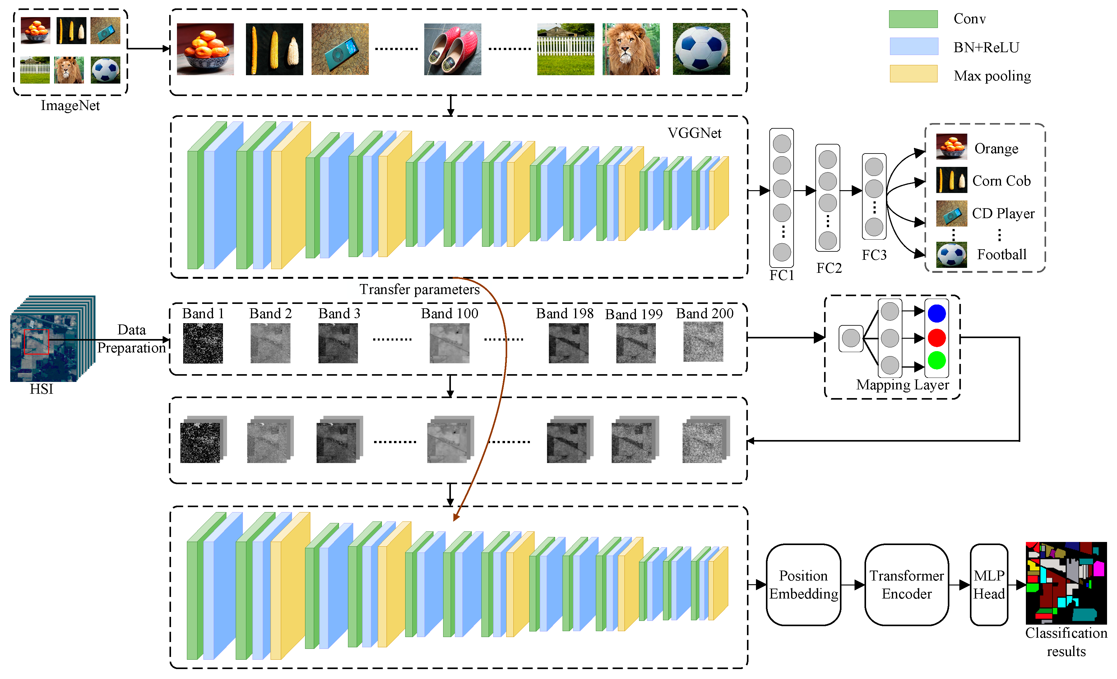
The framework of the proposed SST for HSI classification is shown in
Figure 1. In general, there are three parts in the classification method: CNN-based spatial feature extraction, modified Transformer-based spatial-spectral feature extraction, and MLP-based classification.
Firstly, for each band of HSI, a 2D patch, which contains the neighboring pixels of the pixel to be classified, is selected as input. There are (i.e., the number of bands of HSI) patches for a training sample. After that, a well-designed CNN is used to extract the features of each 2D patch, and then the extracted features are sent to Transformer. Then, the modified Transformer is used to obtain the relationship of the sequential spatial features. At last, the obtained spatial-spectral features are used to get the classification result.
2.1. CNN-Based HSI Spatial Feature Extraction
CNN has powerful capability to extract spatial features of image, and it is widely used for image processing such as classification, detection, and segmentation. For HSI, it contains abundant spatial information. CNN is used in this study to effectively extract the spatial features of HSI.
CNN contains a wide range of different architectures. How to choose a proper architecture is important. Although HSI is a 3-D cube, a 3-D CNN is not used in this study. Instead, a 2-D CNN is used in this classification framework. Furthermore, we use 2-D CNN separately to extract the features of each band in his, and the extracted features are fed into a Transformer.
VGGNet is a simple but effective model, which considers the depth of appropriate layers and does not increase the total number of parameters compared to previous AlexNet [
41]. Therefore, we used VGG-like architecture. The original VGG contains 16 layers, which includes 13 convolutional layers and three fully connected layers. Each convolutional layer is followed by BN layer and ReLU operation, and the max pooling layer is added after the second, fourth, seventh, tenth, and 13th convolutional layer. Possibly, the usage of the whole 16 layers is not a good choice for HSI spatial feature extraction. How to design a proper CNN architecture is a key point for a successful HSI classifier. In the experimental part, we designed a VGG-like deep CNN for spatial feature extraction of HSI.
2.2. Spectral-Spatial Transformer for HSI Classification
CNN uses local connection to extract neighboring features of inputs. HSI usually contains hundreds of bands; therefore, it is difficult for CNN to obtain spectral relationships in a long distance. The self-attention mechanism can obtain the relationship of every two bands. For example, Airborne Visible/Infrared Imaging Spectrometer (AVIRIS) contains 224 bands. Using self-attention, a matrix with the shape of 224 224 can be obtained through the learning procedure. Each element in the matrix represents the relationship between the two bands.
As shown in
Figure 1, the extracted features by CNN in the last part are then sent to the Transformer to learn long-range dependencies, which mainly contains three elements.
The first element is called the position embedding, which aims to capture the positional information of the different bands. This element modifies the output features of the last part, which depends on its positions without changing these full features. In this paper, one dimensional position embedding is utilized, which considers the input features as a sequence of different bands. These generated positional embeddings are added to the features, then sent together to the next element. In addition, a learnable position embedding is prepared (i.e., number zero), whose state serves as the whole representations of the band. This learnable position embedding combines with the third part to finish the classification task.
The second element is the Transformer encoder, which is the core part of our model. The Transformer encoder contains a total of encoder blocks, and each encoder block consists of a multi-head attention and a MLP layer, coupled with layer normalization and residual connection. In each encoder block, a normalization layer is added before each multi-head attention and an MLP layer, and residual connections are designed after each multi-head attention and MLP layer.
Let denote the number of
bands of HSI
by
, where
indicates the dimension of the extracted features by CNN. The Transformer encoder aims to capture the interaction among all
bands of HSI by encoding each band in terms of the global contextual information. Specifically, three learnable weight matrices including queries (i.e.,
), keys (i.e.,
) of dimension
, and values (i.e.,
) of dimension
are defined. The dot products are applied to compute the query with all keys, and then the softmax function is used to compute the weights on the values. The output of attention is defined as follows:
where
is the dimension of
.
It is beneficial to project the queries, keys, and values several times (i.e.,
times) with different and learned projections, and then these results are concatenated. This process is named the multi-head attention. Each result of those parallel computations of attention is called a
head.
where
,
,
,
, and
are parameter matrices.
After that, the weights extracted by the multi-head attention mechanism are sent to the MLP layer, whose output features are 512 dimensions. Here, MLP is constituted by two fully connected layers with a nonlinearity named the Gaussian error linear unit (GELU) activation between. Here, GELU is the variant of the ReLU, which can be defined as follows [
42]:
where
indicates the standard Gaussian cumulative distribution function,
.
Before the MLP layer, there is always a normalization layer [
43], which not only reduces the training time by normalizing neurons, but also alleviates the vanishing or exploding gradient problem. For the
th summed input at the
-th layer
, the normalization layer represents as follows:
where
is normalized summed input, and
and
represent expectation and variance at
th layer, respectively.
and
indicate the learned scale parameter and shift parameter, respectively.
For a deep learning model, there is a common problem titled vanishing-gradient, which hampers the convergence in the training of the deep Transformer model [
40]. To alleviate the vanishing-gradient and strengthen feature propagation, short-cut connection is used to form a DenseTransformer. Specially, each layer in DenseTransformer has connections of the previous layers in the DenseTransformer. For a traditional Transformer
with
layers, there are
connections, and a DenseTransformer has
connections. The DenseTransformer encourages feature reuse and therefore mitigates the vanishing-gradient problem.
Figure 2 shows the proposed DenseTransformer when
= 3.
The proposed DenseTransformer consists of
layers, considering a single
indicates the output of the traditional Transformer
at the
-th layer. Consequently, the
-th layer of the proposed DenseTransformer receives the weights produced by the previous preceding layers
, which can be defined as follows:
where
,
,
,
, and
are parameter matrices.
The third part of SST is MLP. The architecture of MLP includes two fully connected layers with a GELU operation, where the last fully connected layer (i.e., the softmax layer) aims to generate the final results for HSI classification. In softmax, for an input vector
, the probability that the input belongs to category
can be estimated as follows:
where
and
are weights and biases of the Softmax layer, respectively.
In the MLP, the size of the input-layer is set to be the same as the size of the output-layer of the Transformer, and the size of the output-layer is set to be the same as the total number of classes. Softmax ensures the activation of each output unit sums to 1. Therefore, the output can be deemed as a set of conditional probabilities.
2.3. Dynamic Feature Augmentation
Due to the proposed, SST is often susceptible to overfitting and therefore requires proper regularization to generalize well. In this subsection, a simple regularization technique called dynamic feature augmentation is proposed, which is implemented by randomly masking out features during training. Then, SST is combined with feature augmentation to form a new HSI classifier (i.e., SST-FA), which improves the robustness and overall classification performance of SST.
Specially, the dimension of the spatial features extracted by the VGG is high (i.e., 512-dimension), which is easy to overfit for the Transformer model. Here, a coordinate is first randomly selected in the features, then, a mask is placed around the coordinate, which decides how many features are set to zero. Note that the coordinate dynamically changes w.r.t. epochs during training, which ensures the Transformer model receives different features. The proposed SST-FA is not only easy to implement, but also able to further improve the Transformer model performance.
3. Heterogeneous Transferring Spatial-Spectral Transformer for Hyperspectral Image Classification
The collection of training samples is not only expensive but also time-consuming. Therefore, limited training samples are a common issue in HSI classification. To address this issue, transfer learning is combined with SST in this study. Transfer learning is a technique that extracts the knowledge from the source domain and transfers it to the target domain [
44]. For example, in CNN-based transfer learning, the learned weights on the source domain can be used to initialize the net of the target domain. Therefore, when it is properly used, transfer learning can improve the classification performance of the target task if the number of training samples is limited.
To further improve classification performance of the proposed SST, transferring SST (T-SST) is proposed in this section.
Figure 3 shows the framework of the proposed T-SST for HSI classification. In general, there are three parts in the classification method: transferring CNN-based spatial feature extraction, Transformer-based spatial-spectral feature extraction, and MLP-based classification.
3.1. Heterogeneous Mapping of Two Datasets
There is a problem of simply using transfer learning for HSI classification, due to the fact that the large-scale dataset (i.e., the source dataset) has three channels, but HSI (i.e., the target dataset) contains hundreds of channels. To solve the problem caused by heterogeneous transfer learning, a mapping layer is used to handle the issue of different number of channels (i.e., bands) of the two datasets.
The pre-trained model on the large-scale ImageNet dataset has three channels of input (i.e., R, G, and B), but CNN in T-SST receives one band as input.
Let
be the input of CNN, in which
represents the weight and height of a 2D patch.
is the mapped data for subsequent processing, and
. Therefore,
There are three learnable parameters in the heterogeneous mapping. The mapping operation is combined with subsequent CNN to form an end-to-end learning system.
3.2. The Proposed T-SST for HSI Classification
Transfer learning is a technique that aims at extracting knowledge from the source domain and applying it to the target domain [
44]. The learned knowledge from the source task is used to improve the performance of the target task. In deep learning-based transfer learning, deep models can learn a lot of knowledge from a large dataset such as ImageNet, and the learnt knowledge can be transferred to a new task such as HSI classification. Therefore, the proper usage of transfer learning may reduce the number of necessary training samples.
Many previous studies proved that the learnt weights in CNN of the original domain can be re-used in the new task [
45]. For an image classification task, the first several layers usually extract low-level features (i.e., blobs, corners, and edges), and the low-level features are usually common in image classification tasks. Due to the similarity tasks between the ImageNet and HSI classification, the transfer learning step can be facilitated by fine-tuning on HSI classification task. Specifically, the learned weights of VGGNet on the ImageNet dataset can be utilized to initialize the network of the HSI classification and then fine-tune the weights on an HSI classification task.
Here, a new classification framework titled T-SST is proposed for HSI classification, which is a combination of transferred VGGNet, modified Transformer (i.e., DenseTransformer), and MLP. In T-SST, VGGNet with 16 layers is used, which was trained on the ImageNet dataset, and the well-trained weights of all the convolutional layers from the source task are transferred to our target task. Then, these initialized weights are fine-tuned on the HSI dataset.
Using transferred VGGNet, more robust and discriminant features can be extracted compared with the original VGGNet, which is useful for the following processing. The obtained features using transferred VGGNet are used as inputs of Transformer. Specially, a 2D patch, which contains the neighboring pixels in a band of HSI, is an input of transferred VGGNet. VGGNet uses all the convolutional layers to extract the features of the input, then the obtained features are fed into the DenseTransformer. The following MLP is used to obtain the final classification results.
3.3. The Proposed T-SST-L for HSI Classification
Without sufficient training samples, the model faces a problem of “overfitting”, which means that the classification accuracy on test data will be low. This problem is expected when T-SST is applied to HSI classification, because it is a common issue that there are only limited training samples in real application. To address the overfitting issue in T-SST, label smoothing is introduced.
In classification, each training sample
has the corresponding label
.
is the number of classes. Here, we use a
-dimensional one-hot vector
to represent the label of training sample
,
where
,
represents the discrete Dirac delta function, which equals 1 for
and 0 otherwise.
However, work in [
46] has shown that, if we assign all ground truth labels as “hard labels” (i.e., the
), the model will struggle with many efforts to push the predicted distribution of labels towards the hard label. Moreover, this can be effectively relieved if the labels are properly smoothed, i.e., assigned tiny probability mass on the zeros in
. Intuitively, this happens because the model becomes too confident about its predictions. Thus, in this paper, a mechanism called label smoothing for encouraging the model to be less confident is introduced in this paper to achieve better performance. Label smoothing changes the original label
to
, which can be defined as follows:
where
mixes the label of training sample
and the fixed uniform distribution of the number of
classes;
is the smoothing factor [
47].
By reducing the model to learn the full probability label of each training sample, the label smoothing mechanism can mitigate the overfitting problem and increase the generalization ability of the model in a simple form.
4. Experimental Results
4.1. Hyperspectral Datasets
In this study, the performance of proposed methods is evaluated on three public datasets, including the Salinas, Pavia University (Pavia), and Indian Pines datasets.
Table 1 reports the information of all the datasets including the sensor, number of bands, spatial resolution, pixel size dimension, number of classes, and year of data acquisition. The descriptions of all the datasets are summarized below.
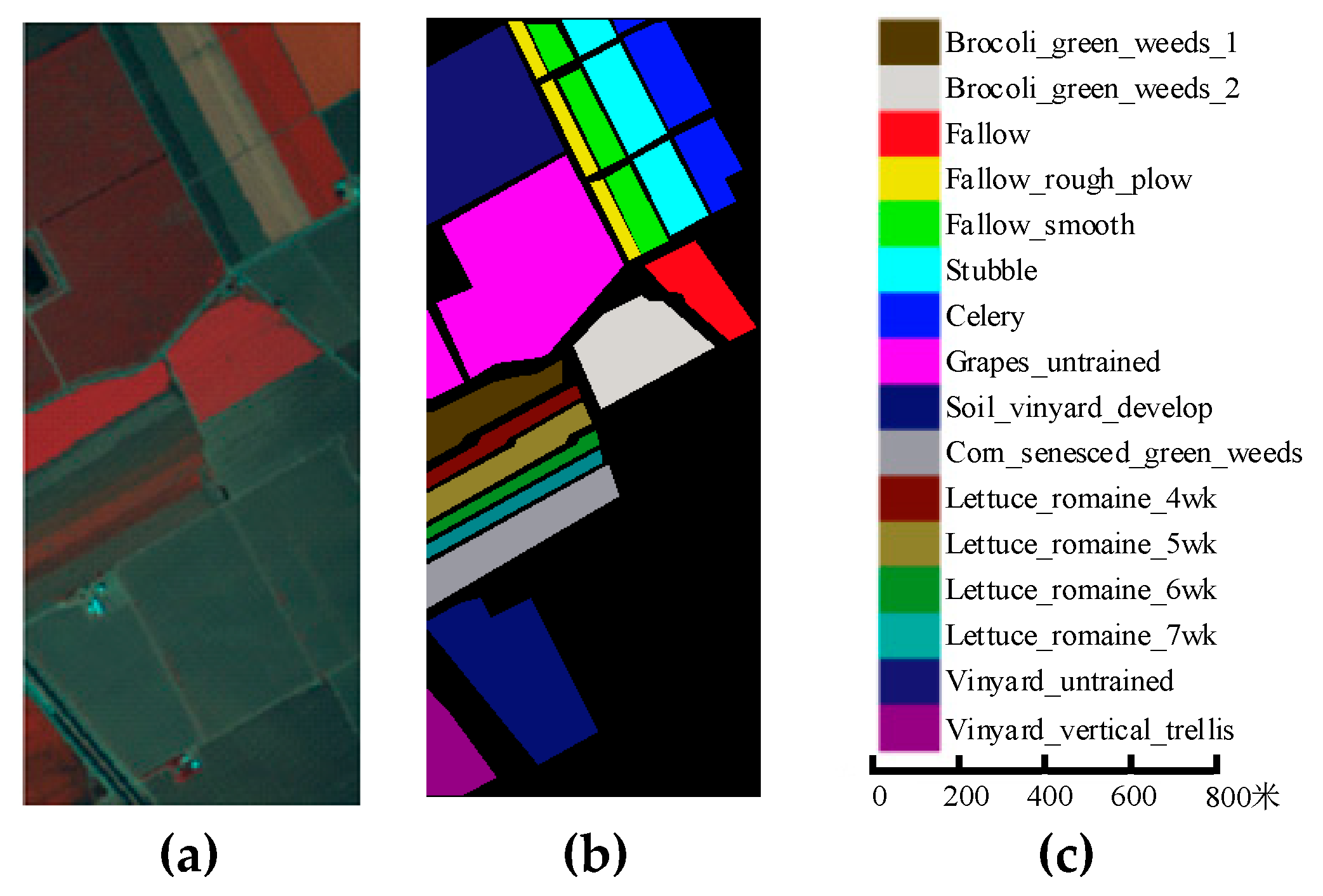
For the Salinas dataset, it was collected by the AVIRIS over Salinas Valley, CA, USA, in 1998. After removing 20 bands of low signal to noise ratio (SNR), 204 bands were used in the experiments.
There are 512
217 pixels with 3.7-m spatial resolution included in this hyperspectral image. The common 16 classes are labeled in the ground truth. The false-color composite image, the available ground-truth map, and the Scale bar are shown in
Figure 4.
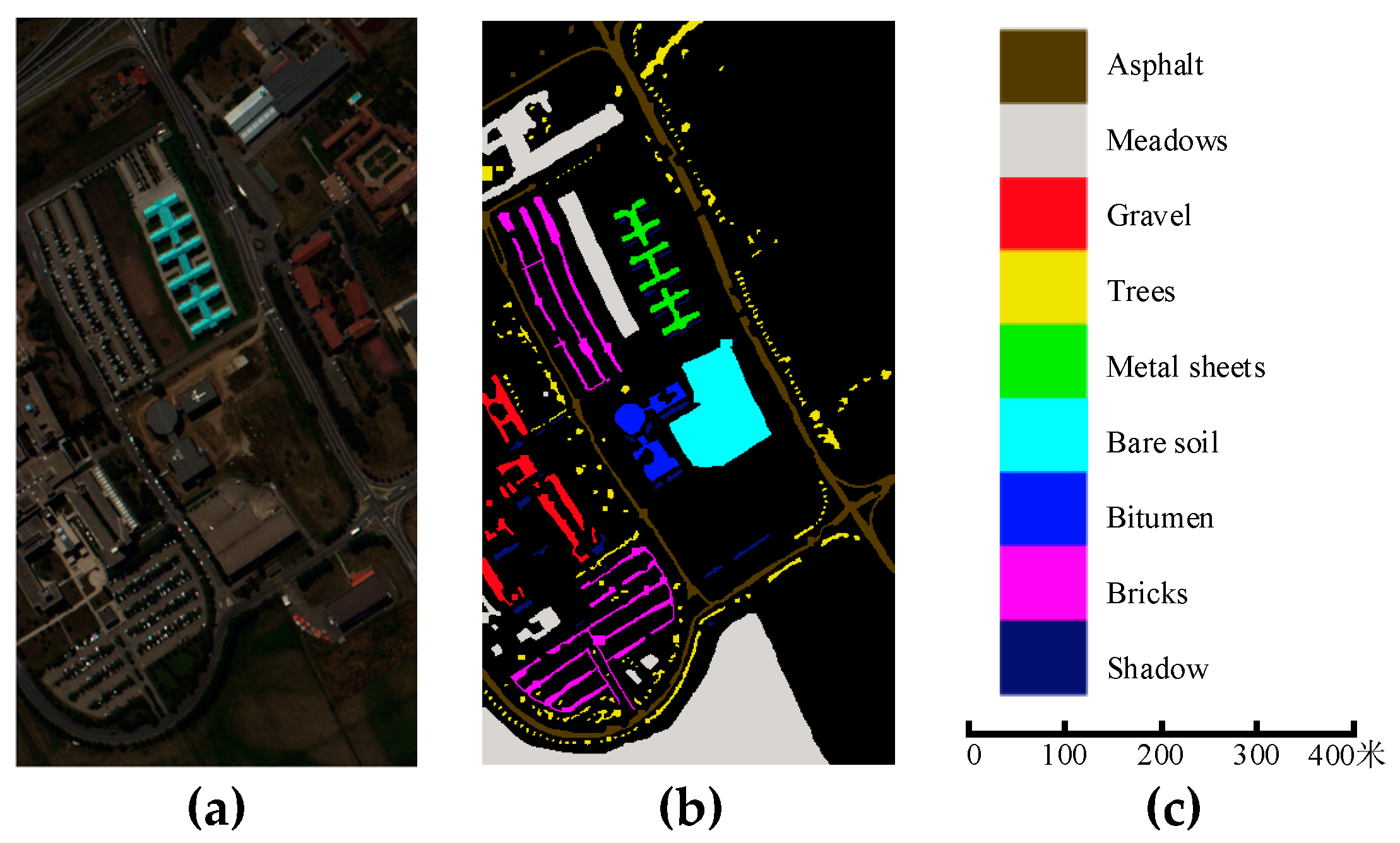
For the Pavia dataset, it was obtained by the Reflective Optics Spectrographic Imaging System (ROSIS) sensor over an urban scene by Pavia University, Italy, in 2001. This dataset has a size of 610
340 pixels with 1.3 m spatial resolution, and the spectral ranges from 0.43 to 0.86 μm. Due to the SNR and water absorption, 12 bands were removed, and the remaining 103 bands were used in the experiments. There are nine urban classes to discriminate.
Figure 5 shows the false-color composite image, the available ground-truth map, and the scale bar.
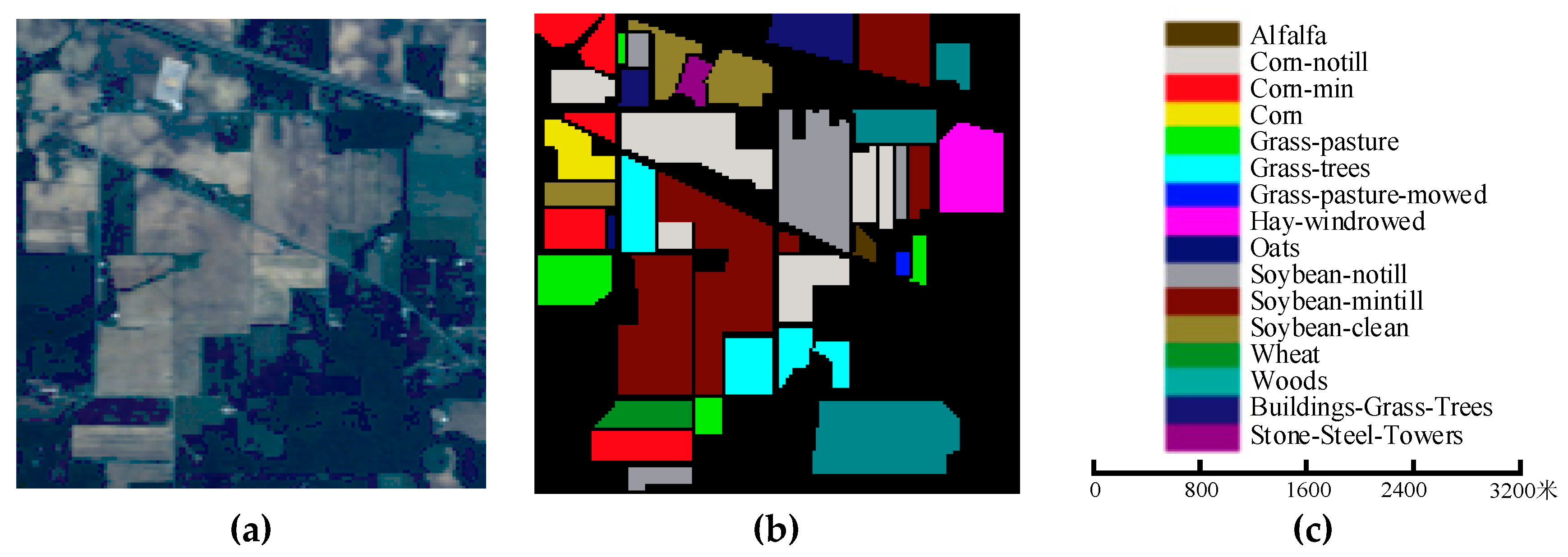
For the Indian Pines dataset, it was captured by the AVIRIS sensor over the Indian Pines region in Northwestern Indiana, 1992. The spatial size of it is 145
145 with the spatial resolution of 20 m. The number of spectral bands is 200 with the wavelengths from 0.4 to 2.5 μm after discarding 20 water absorption bands. Sixteen ground truth classes are labeled in the available ground truth. The false-color composite image, the available ground-truth map, and the scale bar are shown in
Figure 6.
Each dataset is divided into three subsets: training set, validate set, and test set. The training set consists of 200 labeled samples for model training, which are randomly selected from all the labeled samples, the validate set includes 50 labeled samples for guiding the model, and the remains are used as the test set.
The input HSI datasets are normalized into [−0.5, 0.5]. According to
Figure 1, to capture the relationships in a long distance in the spectral domain, the HSI data cube consists of
bands, where the order of bands follows the spectral order. The neighborhood pixels of each sample are set to 33
33, and then these samples are fed into VGGNet.
4.2. Training Details
The VGGNet with 16 layers are adopted in the experiments, which contains 13 convolutional layers and three fully connected layers. The characteristic of VGGNet is mainly adopted small convolutional filters with 3 3 size. Moreover, the 13 convolutional layers can be divided into five groups, and each group contains two or three convolutional layers, which are followed by a max pooling layer. The architecture of VGGNet in SST is similar to VGGNet; to reduce the overfitting for HSI classification, several convolutional layers are ignored, the first three convolutional layer groups reduce one convolutional layer, and the fourth convolutional layer reduces the first two convolutional layers. In addition, for the T-SST, the architecture of VGGNet adopts all the convolutional layers, which are used as initialized weights. For the Pavia and Indian pines datasets, dropout is added. Then, HSI training samples are exploited to fine-tune the VGGNet by the back-propagation algorithm. Due to the input of VGGNet in each band, a mapping layer is designed, whose input is each band and output is three features. Then these features are sent to the VGGNet to extract the discriminative features.
During the training procedure, the mini-batch algorithm is adopted, which is set to 128 for all the datasets [
48]. For the SST, the initial learning rate is set to 8
10
−5 for the Salinas dataset, and 9
10
−5 for the Pavia and Indian Pines datasets, and the learning rate is reduced by 0.9 for each epoch. In the experiments, the small learning rate is found to be suitable for the SST for HSI classification. Additionally, for the T-SST, the learning rate is set to 3
10
−4, 9
10
−5, and 1
10
−4 for the Salinas, Pavia, and Indian Pines datasets, respectively. The learning rate is reduced by 0.7, 0.9, and 0.9 for each epoch for the Salinas, Pavia, and Indian Pines datasets, respectively. Additionally, the training epoch is set to 150 for the Salinas dataset, and for the Pavia and Indian Pines datasets, the training epoch is set to 80. Furthermore, the overall accuracies (OA), average (AA) accuracies, and kappa coefficient (K) are considered to evaluate the performance of different methods.
4.3. Parameter Analysis
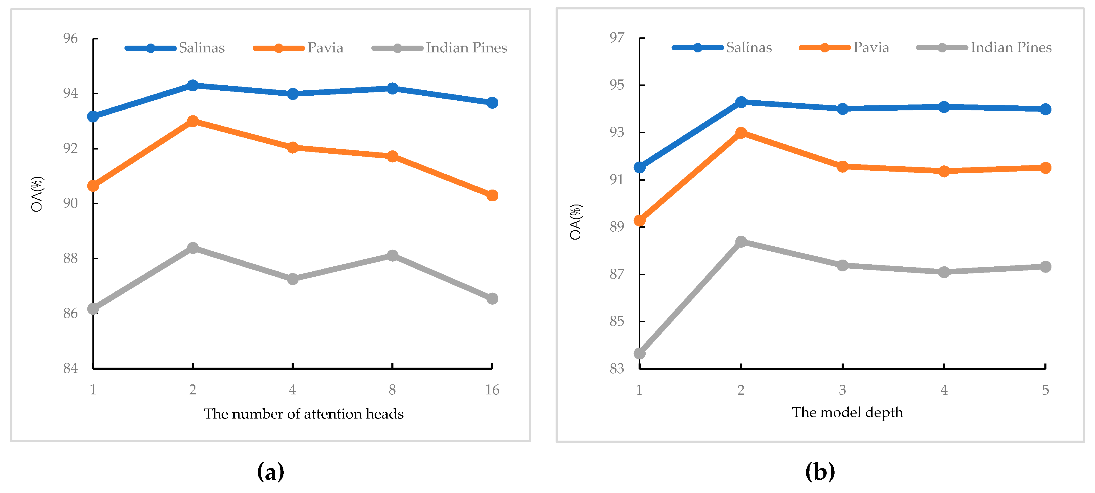
To give a comprehensive study of the spatial-spectral Transformer, some key parameters involved in the Transformer are analyzed in this section, including the number of attention heads, the depth of the Transformer encoder, and the smoothing factor of the proposed T-SST-L. For the number of attention heads and the depth of the Transformer encoder, they not only influence the robustness of the model, but also affect the complexity of the model. With the increment of the model depth, it is easy for the model to encounter the overfitting problem. For the smoothing factor , the value of could influence the performance of the model. Thus, the optimal parameter settings of these parameters are needed to investigate.
To analyze the influences of these parameters to the model, other parameters are fixed; 200 training samples are used for searching optimal parameters.
Figure 7 shows the analysis results evaluated by OA (%) on the Salinas, Pavia, and Indian Pines datasets, respectively. For searching for the optimal number of attention heads, one, two, four, eight, and 16 of attention heads are chosen. This result is shown in
Figure 7a: it can be seen that the best number of attention heads is two for all the datasets. For the depth of the Transformer encoder, the depths ranging from one to five are searched.
Figure 7b shows that the best depth is two for all the datasets: it can be concluded that the lacking depths may cause incomplete information, while for the too deep models, the accuracies are decreased, due to the large amounts of parameters that are needed to train. In the experiments, according to these results, the number of attention heads and depths of the Transformer encoder are set to two for all the datasets to lead to better classification results.
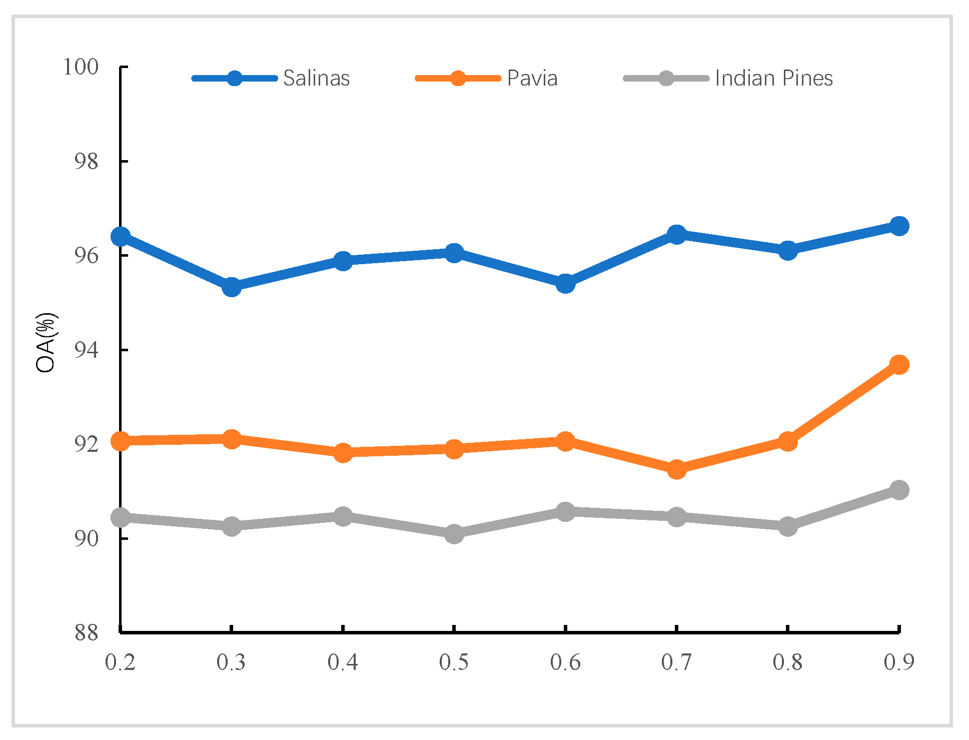
is the smoothing factor of T-SST-L; to validate the influences of T-SST-L with different values of
, the grid search method is utilized to search the optimal value of 𝜀 varying from 0.2 to 0.9. The OA of different values of
is shown in
Figure 8. As can be seen, the OAs of different values of 𝜀 are fluctuant, but the proposed T-SST-L obtains the best result when the value of 𝜀 is set to 0.9 on the three datasets. Therefore, in all experiments, the value of 𝜀 is set to 0.9 for all datasets to obtain the best performance for HSI classification.
4.4. The Classification Results of SST and SST-FA for HSI Classification
In this section, the proposed SST and SST-FA are verified by using several comparison experiments, including the traditional methods (i.e., RBF-SVM and EMP-SVM) and the classical CNN related methods (i.e., CNN, SSRN, and VGG). For RBF-SVM, the radial basis function is adopted as the kernel, and a grid search method is used for finding the best value of
and
, which are in the exponentially growing sequence {
,
,…,
}. The best parameters
and
are obtained using five-fold cross-validation. EMP-SVM combines EMP with SVM; for EMP, a disk-shape structure element with an increasing size from two to eight is designed for the opening and closing operations in EMP to extract features. The architectures of CNN and SSRN are implemented following the settings described in [
34,
49], respectively.
The experimental results of SST and SST-FA are reported in
Table 2,
Table 3 and
Table 4. As can be seen, the values of OA, AA, and kappa achieve by the proposed SST-FA are the best, which reach 94.94%, 93.37%, and 88.98% on the Salinas, Pavia, Indian Pines, respectively.
All the experimental results demonstrate that SST-FA reaches the best performance on all the HSI datasets, which has advantages in alleviating the overfitting. For the proposed SST, take the Salinas dataset as an example, compared to the traditional methods, the OA is 11.33% and 6.83% points higher than that of RBF-SVM and EMP-SVM, respectively; the AA is 7.65% and 4.46% points better, respectively, and the kappa is 12.66% and 7.58% points higher. Besides, compared to CNN, OA of SST is improved by 6.02%, 1.33%, and 1.96% on the Salinas, Pavia, and Indian Pines datasets, respectively. In addition, compared to CNN-based methods including SSRN and VGG, for the Indian Pines dataset, the accuracy of the proposed SST achieves 88.77%, which increases of 5.56% and 1.97%, respectively. SST also offers improvement on the Salinas and Pavia datasets.
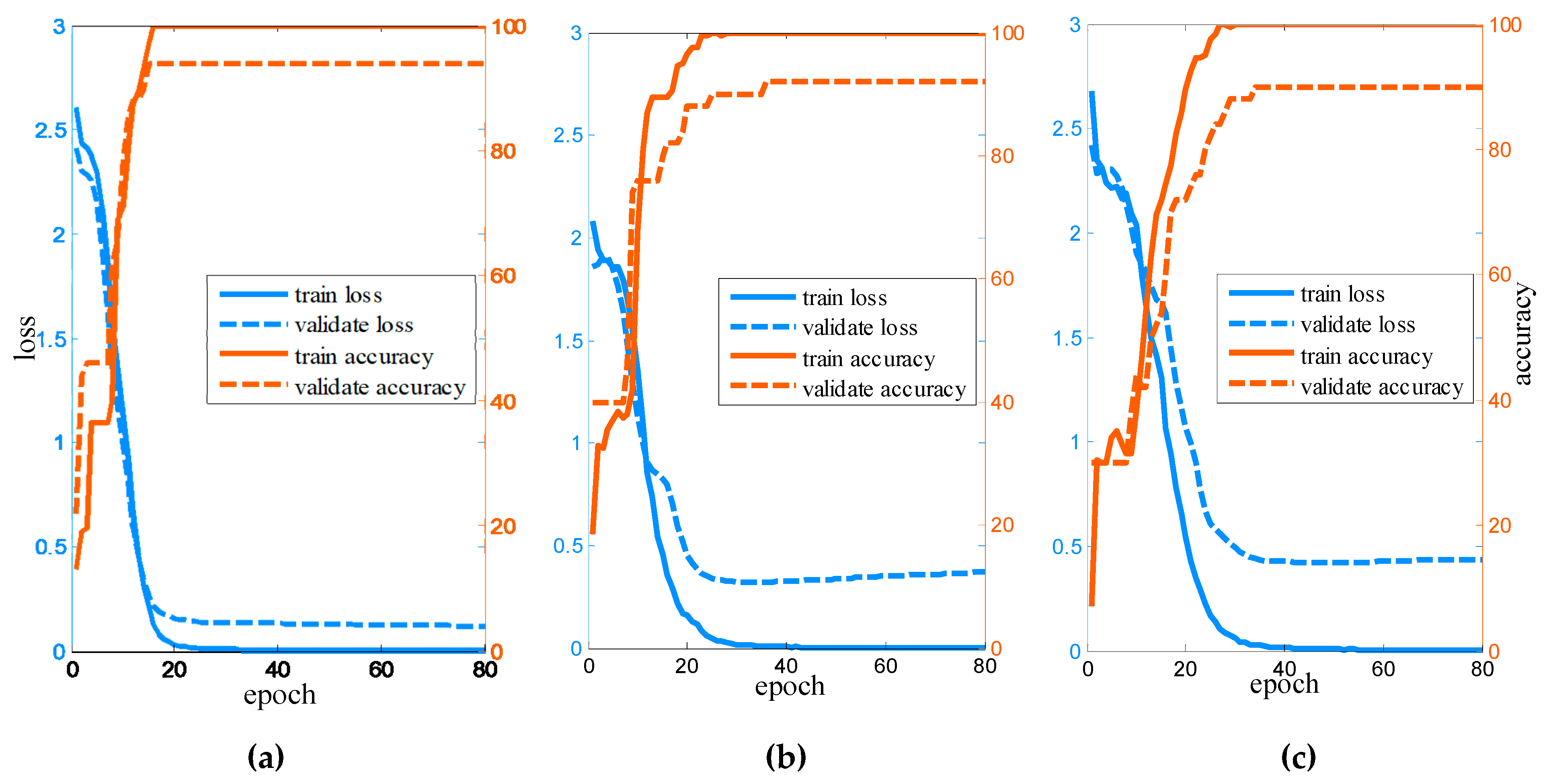
Figure 9 shows learning curves of SST including loss, accuracy of training, and validate samples on the three datasets. The experimental results demonstrate that the proposed SST has the advantages in extracting sequential information of HSI.
4.5. The Classification Results of the Proposed T-SST and T-SST-L for HSI Classification
In this section, the experimental results of the proposed T-SST and T-SST-L are presented to test the performance of HSI classification, which use the pre-trained VGGNet on a large dataset as the initialized weights of VGGNet. To further verify that the proposed T-SST and T-SST-L are superior to other methods for HSI classification, EMP-random forest (RF), EMP-CNN, VGG, and T-CNN are selected for comparison. For EMP-RF, the detailed information about EMP is the same as the previous settings. Then, the features extracted by EMP are fed into the RF classifier with 200 decision trees [
50]. Additionally, EMP-CNN combines EMP with CNN and is implemented for spectral-spatial classification. Specifically, the architecture design of EMP-CNN is similar to CNN [
49]. Moreover, we adopt a comparison method named VGG, whose architecture follows all the convolutional layers in VGGNet; after that, a fully connected layer is added for HSI classification. In addition, to demonstrate the proposed Transformer method with transfer learning is effective, CNN with transfer learning (T-CNN) is also utilized. Three bands are randomly selected from all bands, then all the VGGNet weights of the first seven convolutional layers are used to initialize T-CNN to finish HSI classification task.
The results of the proposed T-SST and T-SST-L are reported in
Table 5,
Table 6 and
Table 7. The proposed T-SST-L achieves competitive results as compared to state-of-the-art well-designed networks. The OA of the proposed T-SST-L reaches 96.83%, 93.73%, and 91.20% on Salinas, Pavia, and Indian Pines datasets, respectively. In addition, it can be observed that the proposed T-SST is superior to other existing methods on all the datasets. Specifically, the T-SST outperforms the EMP-RF by 4.16%, 5.08%, and 4.96% in terms of OA on Salinas, Pavia, and Indian Pines datasets, respectively. Additionally, the accuracy obtained by the proposed T-SST on the Salinas dataset is 3.09% better than that of the EMP-CNN, while, for the Indian Pines dataset, it is 2.84%. In addition, compared to T-CNN, the proposed T-SST achieves about 2% improvements on the Salinas dataset in terms of OA and
. Furthermore, compared to the proposed T-SST, the proposed T-SST-L increases accuracies by 1.03% and 1.14% on Salinas and Indian Pines datasets, respectively. It demonstrates that label smoothing is an effective method to prevent the overfitting problem.
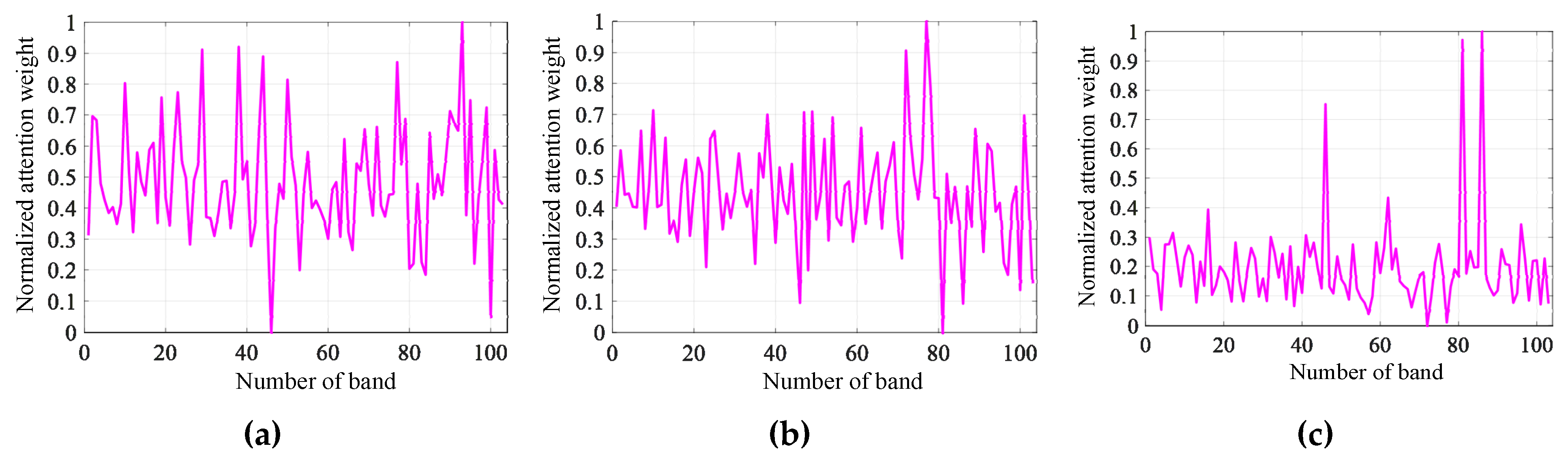
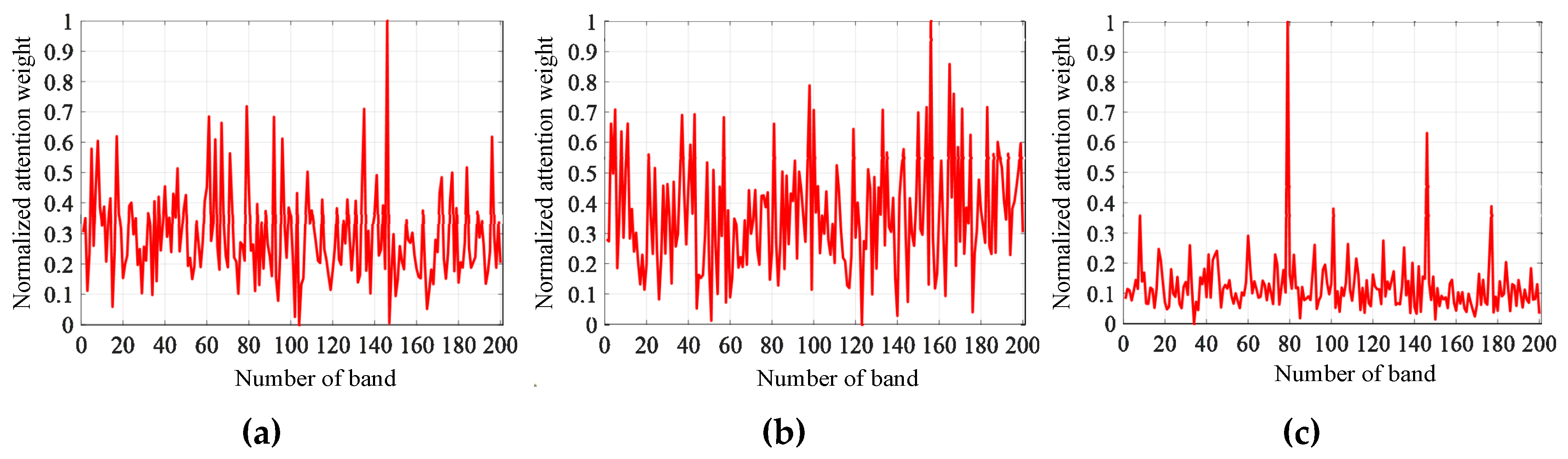
4.6. Analysis of Transformer Encoder Representation of the Proposed T-SST
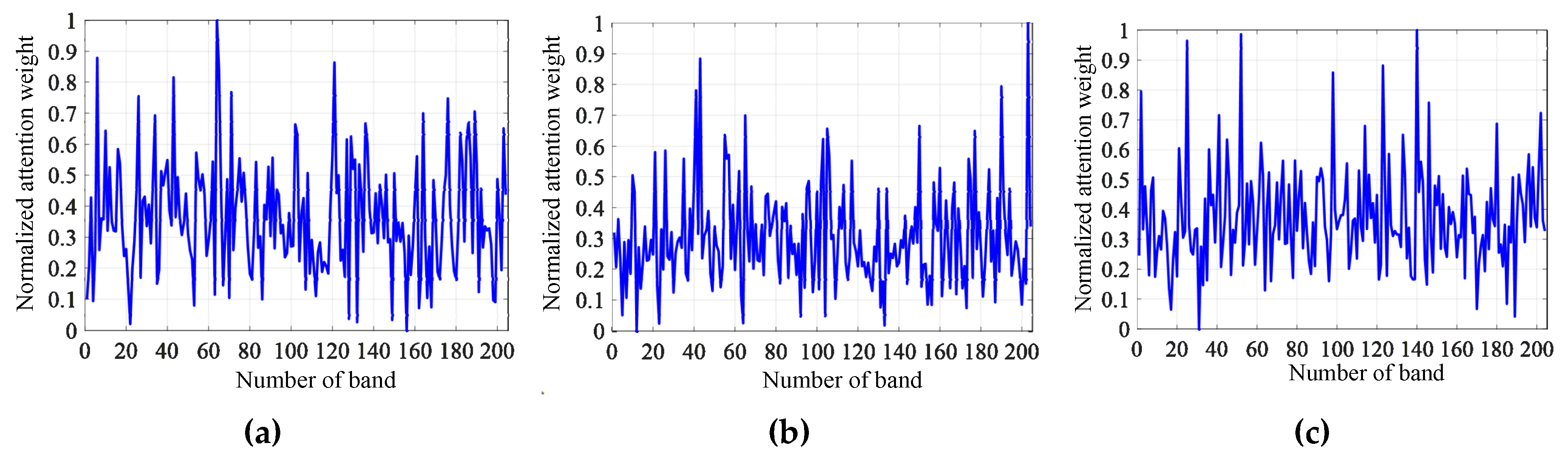
In this subsection, to see how the proposed T-SST captures long-distance dependency relations, we analyze the Transformer encoder representation by visualizing the normalized attention weights.
Figure 10,
Figure 11 and
Figure 12 display normalized attention weights between bands on the three hyperspectral datasets.
Since there are hundreds of bands in HSI, it is difficult to make complete visualization for each of them. Therefore, the first band, the middle band, and the last band are chosen to illustrate the long-range dependency relations between the chosen band and another band. Specially, band 1, band 100, and band 204 are chosen on the Salinas dataset; band 1, band 50, and band 103 are chosen on the Pavia dataset; and band 1, band 100, and band 200 are chosen on the Indian Pines dataset.
As shown in
Figure 10,
Figure 11 and
Figure 12, the values of attention weight strongly fluctuate on the three hyperspectral datasets, and the value of attention weight can be high even if the two bands have a long distance.
Take the Salinas dataset as an example: in
Figure 10a, the value of normalized attention weight between band 50 and band 203 is very high, although distance of the two bands is far. The results demonstrate that T-SST tends to capture long-range dependency relations.
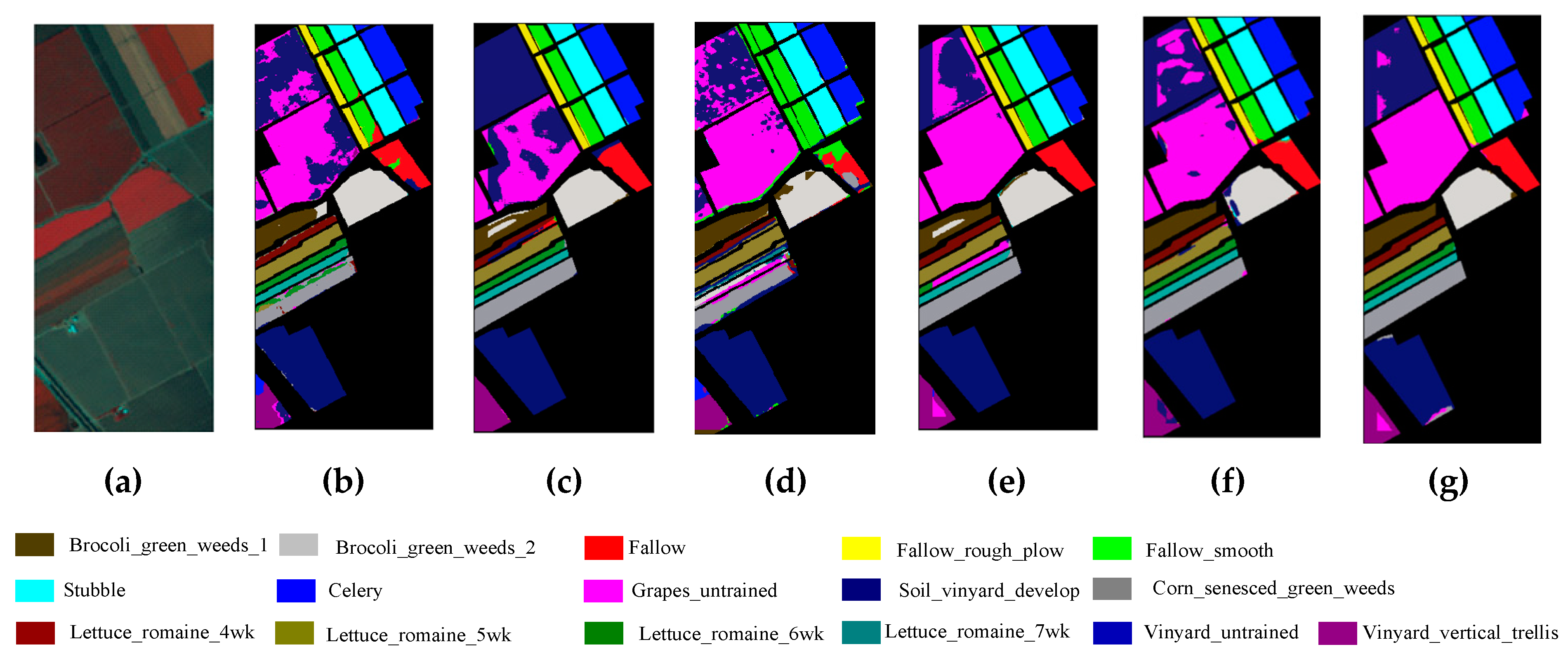
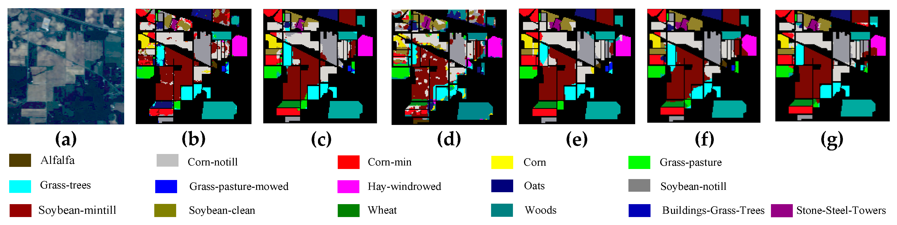
4.7. Classification Maps
Here, to fully evaluate the classification results,
Figure 13,
Figure 14 and
Figure 15 display classification maps of different methods from a visual perspective on all the datasets; the methods include EMP-SVM, CNN, SSRN, VGG, and our proposed methods (i.e., SST-FA and T-SST-L). Through comparison, it can be observed that classification maps of EMP-SVM produce more errors for all the datasets, while for the proposed SST and T-SST, there exist fewer noise points. In addition, in
Figure 15, compared to other CNN-based methods, for example, in comparison of CNN, SSRN, and VGG (see
Figure 15b–d), many pixels are misclassified on the boundary among different classes on the Indian Pines dataset, while the proposed methods are able to classify more classes correctly (i.e., Soybean-clean) and have a clearer distinction. Obviously, SST-FA and T-SST-L produce classification maps with the highest quality compared to other approaches, which demonstrates that the proposed SST-FA and T-SST-L are effective in enhancing the performance of model, respectively.
4.8. Time Consumption
The execution time of different methods for the three HSI datasets with 200 training samples is reported in
Table 8. All the experiments are conducted on a computer with an Intel Core i7-10700F processor with 2.9 GHz, 64 GB of DDR4 RAM, an NVIDIA GeForce RTX 3070 graphical processing unit (GPU). For the traditional methods including RBF-SVM, EMP-SVM, and EMP-RF, the processing time is short, but these methods achieve poor performance. In addition, for the CNN and T-CNN, since CNN includes fewer parameters than other competitive deep-learning-based methods and T-CNN only contains three bands for transfer learning, the running time is short. Additionally, compared to CNN, SSRN and VGG take longer time, because SSRN needs more epochs to train the network and VGG contains many 3 × 3 convolutional kernels. For the proposed methods (i.e., SST, T-SST, and T-SST-L), since the proposed methods consider the model of Transformer, the processing times are long.
5. Conclusions
In this study, Transformer is investigated for HSI classification. Specifically, DenseTransformer is proposed, which uses dense connection to alleviate the vanishing-gradient problem in the training of a Transformer.
Moreover, two classification frameworks (i.e., SST and T-SST) have been proposed to handle the task of HSI classification. The proposed methods obtained superior performance in terms of classification accuracy on the three popular HSI datasets.
For the proposed SST-based HSI classification method, it took full advantage of CNN to capture spatial features of a 2D patch and made best of DenseTransformer to capture relationships in a long distance in spectral domain. The used self-attention mechanism considered the intrinsic sequential data structure of a pixel vector of his, and the combination of CNN and DenseTransformer obtained the spectral-spatial discriminate features, which are useful for the following HSI classification.
In addition, DenseTransformer combined with dynamic feature augmentation (i.e., SST-FA) is proposed for alleviating the overfitting problem, and thus it enhances the accuracy of the model in a simple form.
Furthermore, the effectiveness of T-SST has been tested. The proposed T-SST combined transfer learning and SST to further improve the classification performance. To use the pre-trained model on the ImageNet dataset, a heterogeneous mapping layer was designed, which was used to map the model from the source domain (i.e., ImageNet dataset) to target domain (i.e., HSI). The obtained experimental results have shown the usefulness of T-SST for HSI classification.
At last, label smoothing has been proved as a useful regularization technique in Transformer-based HSI classification. The proposed T-SST-L led to high performance compared to SST, SST-FA, T-SST, and other methods.
The proposed SST and T-SST have shown the potential of the proposed DenseTransformer for HSI classification. However, it is in the early stage of Transformer-based HSI classification. In our future work, various improvements of Transformer can be used to open a new widow for HSI accurate classification.


