Maximum Likelihood Estimation Based Nonnegative Matrix Factorization for Hyperspectral Unmixing

Abstract

Hyperspectral unmixing (HU) is a research hotspot of hyperspectral remote sensing technology. As a classical HU method, the nonnegative matrix factorization (NMF) unmixing method can decompose an observed hyperspectral data matrix into the product of two nonnegative matrices, i.e., endmember and abundance matrices. Because the objective function of NMF is the traditional least-squares function, NMF is sensitive to noise. In order to improve the robustness of NMF, this paper proposes a maximum likelihood estimation (MLE) based NMF model (MLENMF) for unmixing of hyperspectral images (HSIs), which substitutes the least-squares objective function in traditional NMF by a robust MLE-based loss function. Experimental results on a simulated and two widely used real hyperspectral data sets demonstrate the superiority of our MLENMF over existing NMF methods.

1. Introduction

A hyperspectral image (HSI) can be represented as a three-dimensional data cube, containing both spectral and spatial information to characterize radiation properties, spatial distribution and geometric characteristics of ground objects [1,2]. Compared with panchromatic, RGB and multispectral pictures that have only several broad bands, HSI usually has hundreds of spectral bands. The rich spectral information of HSI can be used to discriminate subtle differences between similar ground objects, which makes HSI suitable for different applications, such as target recognition, mineral detection, precision agriculture [1,2,3]. Due to the scattering of ground surface and low spatial resolution of the hyperspectral sensor, an observed HSI pixel is often a mixture of multiple ground materials [4,5,6]. This is the so called “mixed pixel”. The presence of “mixed pixels” seriously affects the application of HSIs. To address the problem of mixed pixels, hyperspectral unmixing (HU) techniques have been developed [4,5,6,7,8]. HU aims to decompose a mixed spectral into a collection of pure spectra (endmembers) while also providing the corresponding fractions (abundances). In terms of the spectral mixture mechanism, HU algorithms can be roughly categorized into linear and non-linear ones [4,5]. Although, in general, the nonlinear mixing assumption represents the most-real cases better, the linear mixing assumption (although more simplified) has been proved to work very satisfactory in many cases in practice. Taking into account its mathematical tractability, it has attracted significant attention from the scientific community. For these reasons, the linear mixture model is adopted in the present paper, in which a measured spectral can be represented as a linear combination of several endmembers.

Nonnegative matrix factorization (NMF) is a widely used linear HU method [9,10,11,12,13,14,15,16,17,18,19,20]. In this framework, HU is regarded as a blind source separable problem, and decomposes an observed HSI matrix into the product of the pure pixel matrix (endmember matrix) and corresponding proportion matrix (abundance matrix). Respecting the physical constraints, nonnegative constraints on the endmembers and abundances, and abundance sum-to-one constraint (ASC) are imposed. The NMF algorithm has the characteristics of intuition and interpretability. However, due to the existence of large number of unknown dependent variables, the solution space of NMF model is too large. To restrict its solution space, many NMF variants are proposed by adding constraints on the abundance or endmember [10,11,12,13,14,15,16]. Miao et al. incorporated a volume constraint of endmember into the NMF formulation and proposed a minimum volume constrained NMF (MVC-NMF) model [10], which can perform unsupervised endmember extraction from highly mixed image data without the pure-pixel assumption. Jia et al. introduced two constraints to the NMF [11], i.e., piecewise smoothness of spectral data and sparseness of abundance fraction. Similarly, two constraints on abundance (i.e., abundance separation constraint and abundance smoothness constraint) were added into the NMF [12]. Qian et al. imposed an $l_{1/2}$-norm-based sparse constraints on the abundance and proposed an $l_{1/2}$-NMF unmixing model [13]. Lu et al. considered the manifold structure of HSI and incorporated manifold regularization into the $l_{1/2}$-NMF [14]. Wang et al. added endmember dissimilarity constraint into the NMF [15].

Although the aforementioned NMF methods improved the classical NMF unmixing model at a certain extent, they ignored the effect of noise. As the objective function of NMF is the least squares loss, NMF is sensitive to noise and corresponding unmixing results are usually inaccurate and unstable. To suppress the effect of noise and improve the robustness of the model, many robust NMF methods were proposed [17,18,19,20]. He et al. proposed a sparsity-regularized robust NMF by adding a sparse matrix into the linear mixture model to model the sparse noise [17]. Du et al. introduced a robust entropy-induced metric (CIM) and proposed a CIM-based NMF (CIM-NMF) model, which can effectively deal with non-Gaussian noise [18]. Wang et al. proposed a robust correntropy-based NMF model (CENMF) [19], which contained a correntropy-based loss function and an $l_1$-norm sparse constraint on the abundance. Based on the Huber’s M-estimator, Huang et al. constructed $l_{2,1}$-norm and $l_{1,2}$-norm based loss functions to obtain a new robust NMF model [20,21]. Defining the $l_{2,1}$-norm ($l_{1,2}$-norm) based loss function actually assumes that the column-wise (row-wise) approximation residual follows Laplacian (Gaussian) distribution from the viewpoint of maximum likelihood estimation (MLE). However, in practice this assumption may not hold well, especially when HSI contains complex mixture noise, such as impulse noise, stripes, deadlines, and other types of noise [22,23].

Inspired by the robust regression theory [23,24], we design the approximation residual as an MLE-like estimator and propose a robust MLE-based $l_{1/2}$-NMF model (MLENMF) for HU. It replaces the least-squares loss in the original NMF by a robust MLE-based loss, which is a function (associated with the distribution of the approximation residuals) of the approximation residuals [24]. The proposed MLENMF can be converted to a weighted $l_{1/2}$-NMF model and can be solved by a re-weighted multiplication update iteration algorithm [9,13]. By choosing an appropriate weight function, MLENMF can automatically assign small weights to bands with large residuals, which can effectively reduce the effect of noisy bands and improve the unmixing accuracy. Experimental results on simulated and real hyperspectral data sets show the superiority of MLENMF over existing NMF methods.

The rest of the paper is organized as follows. Section 2 introduces the NMF and $l_{1/2}$-NMF. Section 3 describes our proposed MLENMF method. The experimental results and analysis are provided in Section 4. Section 5 discusses the effect of parameters in the algorithm. Finally, Section 6 concludes the paper.

2. NMF Unmixing Model

Under the linear spectral mixing mechanism, an observed spectral $\mathit{h}\in R^{M\times 1}$ can be represented linearly by the endmember ${\mathit{z}}_1,\cdots ,{\mathit{z}}_P$ [4,10,11,12,13]:

$$\mathit{h}=\mathit{Z}\mathit{s}+\mathit{ϵ},$$

(1)

where $\mathit{Z}=\left[{\mathit{z}}_1,\cdots ,{\mathit{z}}_P\right]\in R^{M\times P}$ represents the endmember matrix, $\mathit{s}\in R^{P\times 1}$ is the coefficient (abundance) vector, and $\mathit{ϵ}$ is the residual. Applying the above linear mixing model (1) for all hyperspectral pixels ${\mathit{h}}_1,\cdots ,{\mathit{h}}_N$, the following matrix representation can be obtained:

$$\mathit{H}=\mathit{Z}\mathit{S}+\mathit{E},$$

(2)

where $\mathit{H}=\left[{\mathit{h}}_1,\cdots ,{\mathit{h}}_N\right]\in R^{M\times N}$, $\mathit{S}=\left[{\mathit{s}}_1,\cdots ,{\mathit{s}}_N\right]\in R^{P\times N}$ are nonnegative hyperspectral data matrix and abundance matrix, respectively. $\mathit{E}\in R^{M\times N}$ is the residual matrix.

In Equation (2), to make the decomposition result as accurate as possible, the residual should be minimized. Then, an NMF unmixing model can be obtained by considering the nonnegative property of endmember and abundance matrices:

$$\underset{\mathit{Z},\mathit{S}}{\min } {\Vert \mathit{H}-\mathit{Z}\mathit{S}\Vert }_F^2, \mathrm{s}.\mathrm{t}., \mathit{Z}\ge 0,\mathit{S}\ge 0,$$

(3)

where ${\Vert ·\Vert }_F$ denotes the Frobenius norm, and $\mathit{Z}\ge 0$ means that each element of $\mathit{Z}$ is nonnegative. As each column of abundance matrix $\mathit{S}$ records the proportion of endmembers in representing a pixel, the columns of $\mathit{S}$ (each one corresponding to a pixel) should satisfy the sum-to-one constraint, i.e., ${\sum }_{p=1}^P{S}_{pn}=1, n=1,\cdots ,N$.

The above NMF Model (3) can be easily solved by the multiplication update algorithm [9,13]. However, its solution space is very large [13]. To restrict the solution space, an $l_{1/2}$-constraint can be added to the abundance matrix $\mathit{S}$, and an $l_{1/2}$-NMF model can be obtained as [13]:

$$\underset{\mathit{Z},\mathit{S}}{\min } {\Vert \mathit{H}-\mathit{Z}\mathit{S}\Vert }_F^2+\lambda {\Vert \mathit{S}\Vert }_{1/2}, \mathrm{s}.\mathrm{t}., \mathit{Z}\ge 0,\mathit{S}\ge 0,$$

(4)

where $\lambda$ is a regularization parameter and ${\Vert \mathit{S}\Vert }_{1/2}$ is the $l_{1/2}$-regularizer [13]. As proved in Refs. [13,25], $l_{1/2}$-regularizer is a good choice in enforcing the sparsity of hyperspectral unmixing because the sparsity of the $l_q$ ($1/2\le q<1$) solution increases as $q$ decreases, whereas the sparsity of the solution for $l_q$ ($0<q\le 1/2$) shows little change with respect to $q$. Meanwhile, the sparsity represented by $l_{1/2}$ also enforces the volume of the simplex to be minimized [13].

3. MLENMF Unmixing Model

In the NMF model (3) or (4), the objective function ${\Vert \mathit{H}-\mathit{Z}\mathit{S}\Vert }_F^2$ is the least-squares (LS) function which is sensitive to noise. Here, we employ a new robust MLE-based loss to replace the LS objective function and propose an MLE-based NMF (MLENMF) model for HU.

Firstly, the matrix norm form is transformed into vector norm form:

$${\Vert \mathit{H}-\mathit{Z}\mathit{S}\Vert }_F^2={\displaystyle \sum _{i=1}^M}{\Vert {\mathit{H}}^i-{\left(\mathit{Z}\mathit{S}\right)}^i\Vert }_2^2,$$

(5)

where ${\mathit{H}}^i$ is the $i$-th row of matrix $\mathit{H}$.

We can regard the least squares objective function as the sum of approximation residuals, and then construct an MLE-like robust estimator to approximate the minimum of objective function. Denote the approximation residual of the $i$-th band as $e_i={\Vert {\mathit{H}}^i-{\left(\mathit{Z}\mathit{S}\right)}^i\Vert }_2$ and define residual vector $e={\left[e_1, \dots , e_M \right]}^T$, the above Formula (5) can be rewritten as:

$$J\left(\mathit{e}\right)={\Vert \mathit{e}\Vert }_2^2={\displaystyle \sum _{i=1}^M}{e}_i^2.$$

(6)

Assume that $e_1, \dots , e_M$ are independent and identically distributed (i.i.d) random variables, which follow the same probability distribution function $g_{\theta }\left(e_i\right)$, where $\theta$ is the distribution parameter. The likelihood function can be expressed as:

$$J_{\theta }\left(e_1, \dots , e_n\right)={\displaystyle \prod _{i=1}^M}{g}_{\theta }(e_i).$$

(7)

According to the principle of MLE, the following objective function should be minimized:

$$-\ln J_{\theta }={\displaystyle \sum _{i=1}^M} {\phi }_{\theta }\left(e_i\right),$$

(8)

where ${\phi }_{\theta }\left(e_i\right)=-\ln g_{\theta }\left(e_i\right)$. If we replace the objective function ${\Vert \mathit{H}-\mathit{Z}\mathit{S}\Vert }_F^2$ in Equation (4) by the loss in Equation (8), we can get the following optimization problem:

$$\underset{\mathit{Z},\mathit{S}}{\min }{\displaystyle \sum _{i=1}^M}{\phi }_{\theta }\left(e_i\right)+\lambda {\Vert \mathit{S}\Vert }_{1/2}, \mathrm{s}.\mathrm{t}., \mathit{Z}\ge 0,\mathit{S}\ge 0,$$

(9)

In fact, the aim is to construct a loss function to replace the least squares function to reduce the impact of noise. To construct the loss function, we analyze its Taylor expansion. Assume that $g_{\theta }$ is symmetric, and $g_{\theta }\left(e_i\right)<g_{\theta }\left(e_j\right)$ if $\left|e_i\right|>\left|e_j\right|$. We can infer that: (1) $g_{\theta }\left(0\right)$ is global maximum of $g_{\theta }$ and ${\phi }_{\theta }\left(0\right)$ is the global minimum of ${\phi }_{\theta }$; (2) ${\phi }_{\theta }\left(e_i\right)={\phi }_{\theta }\left(-e_i\right)$; (3) ${\phi }_{\theta }\left(e_i\right)>{\phi }_{\theta }\left(e_j\right)$ if $\left|e_i\right|>\left|e_j\right|$. For simplicity, we assume ${\phi }_{\theta }\left(0\right)=0$. Define $D_{\theta }\left(\mathit{e}\right)={\sum }_{i=1}^M{\phi }_{\theta }\left(e_i\right)$. According to the first-order Taylor expansion around ${\mathit{e}}_0$, $D_{\theta }\left(\mathit{e}\right)$ can be approximated as [24]:

$${\tilde{D}}_{\theta }\left(\mathit{e}\right)=D_{\theta }\left({\mathit{e}}_0\right)+{\left(\mathit{e}-{\mathit{e}}_0\right)}^T{D}_{\theta }^{\prime }\left({\mathit{e}}_0\right)+\frac{1}{2}{\left(\mathit{e}-{\mathit{e}}_0\right)}^T\mathit{W}\left(\mathit{e}-{\mathit{e}}_0\right),$$

(10)

where $D_{\theta }^{\prime }\left({\mathit{e}}_0\right)$ is the first order derivative of $D_{\theta }\left(\mathit{e}\right)$ at ${\mathit{e}}_0$, and $\mathit{W}$ is the Hessian matrix. We can get the mixed partial derivatives $\frac{{\partial }^2{D}_{\theta }}{\partial e_i\partial e_j}=0$ ($e_i\ne e_j$) as the error residuals $e_i$ and $e_j$ are assumed i.i.d., and hence $\mathit{W}$ is a diagonal matrix. Taking the derivative of ${\tilde{D}}_{\theta }\left(\mathit{e}\right)$ with respect to $\mathit{e}$, it gets

$${\tilde{D}}_{\theta }^{\prime }\left(\mathit{e}\right)=D_{\theta }^{\prime }\left({\mathit{e}}_0\right)+\mathit{W}\left(\mathit{e}-{\mathit{e}}_0\right).$$

(11)

As ${\phi }_{\theta }\left(0\right)=0$ is the global minimum of ${\phi }_{\theta }$, the minimum of $D_{\theta }\left(\mathit{e}\right)$ is $D_{\theta }\left(\mathbf{0}\right)$. ${\tilde{D}}_{\theta }\left(\mathit{e}\right)$ should also reach its minimum at $\mathit{e}=\mathbf{0}$ for it is an approximation of $D_{\theta }\left(\mathit{e}\right)$, so ${\tilde{D}}_{\theta }^{\prime }\left(\mathbf{0}\right)=0$ and then we can derive the following formulas from Equation (11):

$$D_{\theta }^{\prime }\left({\mathit{e}}_0\right)-\mathit{W}{\mathit{e}}_0=0$$

(12)

$$W_{i,i}=\frac{{\phi }_{\theta }^{\prime }\left(e_{0,i}\right)}{e_{0,i}}$$

(13)

where $W_{i,i}$ is the $i$-th diagonal element of $\mathit{W}$. Denote $w_i=W_{i,i}$, Equation (13) can be written as

$${\phi }_{\theta }^{\prime }\left(e_i\right)=w_i{e}_i$$

(14)

As ${\phi }_{\theta }\left(x\right)$ is a nonlinear and nonconvex function, it is difficult to solve the model (9) directly. Inspired by the above Formula (14), we can get:

$${\phi }_{\theta }\left(e_i\right)=w_i{e}_i^2,$$

(15)

and then the Model (9) can be expressed as a weighted NMF model:

$$\underset{\mathit{Z},\mathit{S}}{\min }{\displaystyle \sum }_{i=1}^M{w}_i{e}_i^2+\lambda {\Vert \mathit{S}\Vert }_{1/2}, \mathrm{s}.\mathrm{t}., \mathit{Z}\ge 0,\mathit{S}\ge 0,$$

(16)

The objective function of Model (16) can be rewritten as:

$$\begin{array}{c}{\displaystyle \sum _{i=1}^M}{w}_i{e}_i^2+\lambda {\Vert \mathit{S}\Vert }_{1/2}={\displaystyle \sum _{i=1}^M}{w}_i{\Vert {\mathit{H}}^i-{\left(\mathit{Z}\mathit{S}\right)}^i\Vert }_2^2+\lambda {\Vert \mathit{S}\Vert }_{1/2}\\ ={\displaystyle \sum _{i=1}^M}{\Vert \sqrt{w_i}{\mathit{H}}^i-{\left(\sqrt{w_i}\mathit{Z}\mathit{S}\right)}^i\Vert }_2^2+\lambda {\Vert \mathit{S}\Vert }_{1/2}\\ ={\Vert \tilde{\mathit{H}}-\tilde{\mathit{Z}}\mathit{S}\Vert }_F^2+\lambda {\Vert \mathit{S}\Vert }_{1/2},\end{array}$$

(17)

where $\tilde{\mathit{H}}=\sqrt{\mathit{W}}\mathit{H}$, $\tilde{\mathit{Z}}=\sqrt{\mathit{W}}\mathit{Z}$. Then, the Model (16) can be expressed as:

$$\underset{\mathit{Z},\mathit{S}}{\min }{\displaystyle \sum _{i=1}^M}{\Vert \tilde{\mathit{H}}-\tilde{\mathit{Z}}\mathit{S}\Vert }_F^2+\lambda {\Vert \mathit{S}\Vert }_{1/2}, \mathrm{s}.\mathrm{t}., \mathit{Z}\ge 0,\mathit{S}\ge 0.$$

(18)

It is easy to see that model (18) is also an $l_{1/2}$-NMF algorithm, and can be solved by the multiplication update iteration rule as follows [9,13]:

$$\tilde{\mathit{Z}}\underset{ }{\leftarrow } \tilde{\mathit{Z}}.\ast \left(\tilde{\mathit{H}}{\mathit{S}}^T\right)./\left(\tilde{\mathit{Z}}\mathit{S}{\mathit{S}}^T\right)$$

(19)

$$\mathit{S}\underset{ }{\leftarrow } \mathit{S}.\ast \left({\tilde{\mathit{Z}}}^T\tilde{\mathit{H}}\right)./\left({\tilde{\mathit{Z}}}^T\tilde{\mathit{Z}}\mathit{S}+\frac{\lambda }{2}{\mathit{S}}^{-\frac{1}{2}}\right)$$

(20)

The final endmember matrix is $\mathit{Z}={\mathit{W}}^{-\frac{1}{2}}\tilde{\mathit{Z}}$.

In the model (18), a key factor is the weight. In this paper, the weight function is set as the logistic function [23,24,26]:

$$w_i\triangleq w\left(e_i\right)=\frac{1}{1+\exp \left(-\gamma \left(\tau -e_i^2\right)\right)}=\frac{\exp \left(\gamma \left(\tau -e_i^2\right)\right)}{1+\exp \left(\gamma \left(\tau -e_i^2\right)\right)},$$

(21)

where $\gamma ,\tau$ are positive scalars. Parameter $\gamma$ controls the decreasing rate from 1 to 0, and $\tau$ controls the location of demarcation point [24]. It is clear that the value of weight function decreases rapidly with the increase of residual $e_i$.

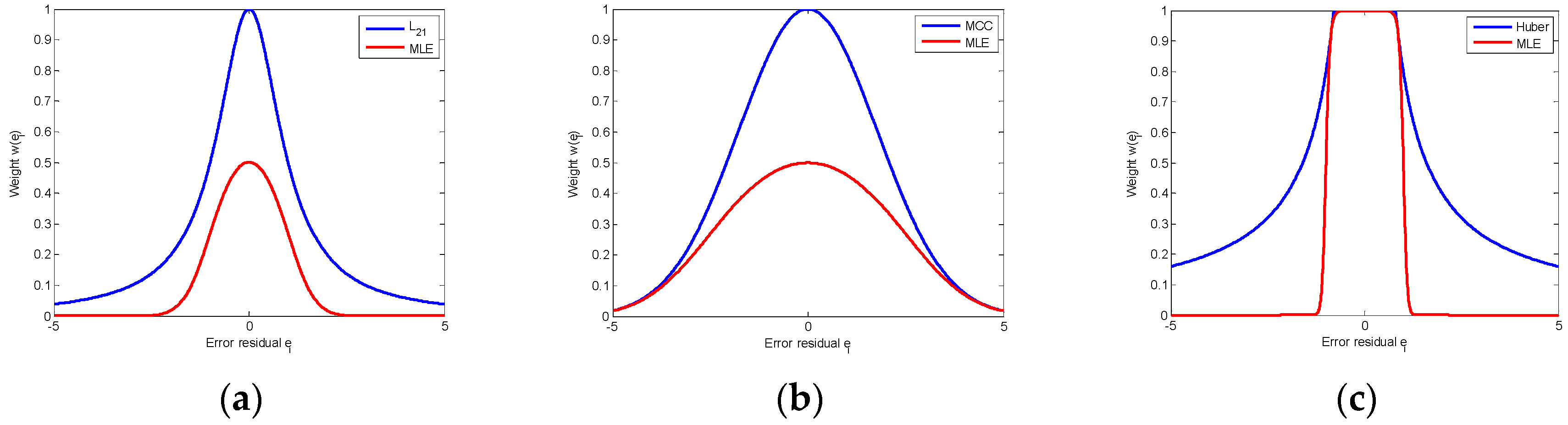
MLE weight function in Equation (21) can approximate the weight of commonly used loss functions, such as $l_{2,1}$, maximum correntropy and Huber weights.

When $\gamma =2$ and $\tau \to 0$, the MLE weight function is:

$$w\left(e_i\right)=\frac{1}{1+\exp \left(2e_i^2\right)} \underrightarrow{for small e_i} \frac{1}{2\left(1+e_i^2\right)}$$

(22)

which is close to $l_{2,1}$ weight: $\frac{1}{1+e_i^2}$. The corresponding weights are shown as red and blue lines in Figure 1a.

When $\gamma =\frac{1}{{\sigma }^2}$ and $\tau \to 0$, the MLE weight function is:

$$w\left(e_i\right)=\frac{1}{\left(1+\exp \left(\frac{e_i^2}{{\sigma }^2}\right)\right)}$$

(23)

which is close to the weight of maximum correntropy criterion: $\exp \left(-\frac{e_i^2}{{\sigma }^2}\right)$ ($\sigma$ is a parameter). The corresponding weights are shown in Figure 1b.

By choosing appropriate parameters, the MLE weight can also approximate the Huber weight:

$$w_{\mathrm{Huber}}\left(e_i\right)=\{\begin{array}{ll}1,& \left|e_i\right|\le c\\ \frac{c}{\left|e_i\right|},& \left|e_i\right|>c\end{array}$$

(24)

as shown in Figure 1c.

Based on Equations (14) and (21), the objective function of MLE can be obtained as:

$$\begin{array}{c}{\phi }_{\theta }\left(e_i\right)={{\displaystyle \int }}_0^{e_i}{\phi }_{\theta }^{\prime }\left(e_i\right)d{e}_i={{\displaystyle \int }}_0^{e_i}{e}_{i}w\left(e_i\right)d{e}_i\\ ={{\displaystyle \int }}_0^{e_i}{e}_i\frac{\exp \left(\gamma \left(\tau -e_i^2\right)\right)}{1+\exp \left(\gamma \left(\tau -e_i^2\right)\right)}d{e}_i\\ =\frac{-1}{2\gamma }\ln \left( 1+\exp \left(\gamma \left(\tau -e_i^2\right) \right)\right){|}_0^{e_i}\\ =\frac{-1}{2\gamma }\ln \frac{1+\exp \left(\gamma \left(\tau -e_i^2\right)\right)}{1+\exp \left(\gamma \tau \right)}\end{array}$$

(25)

From Equations (8) and (25), we can see that the probability distribution function $g_{\theta }\left(e_i\right)$ has the form:

$$g_{\theta }\left(e_i\right)={\left(\frac{1+\exp \left(\gamma \left(\tau -e_i^2\right)\right)}{1+\exp \left(\gamma \tau \right)}\right)}^{\frac{1}{2\gamma }}$$

(26)

If $\tau =0$, $\gamma \to 0$, the probability distribution function $g_{\theta }\left(e_i\right)$ is actually a Gaussian distribution:

$$\ln g_{\theta }\left(e_i\right)=\frac{\ln \frac{1+\exp \left(-\gamma e_i^2\right)}{2}}{2\gamma }\stackrel{\gamma \to 0}{\to }\frac{\exp \left(-\gamma e_i^2\right)·\left(-e_i^2\right)}{1+\exp \left(-\gamma e_i^2\right)} \stackrel{\gamma \to 0}{\to } -\frac{e_i^2}{2}$$

(27)

$$g_{\theta }\left(e_i\right)\stackrel{\gamma \to 0}{\to }\exp \left(-\frac{e_i^2}{2}\right)$$

(28)

In this case, the weight defined in Equation (21) is: ${\omega }_i=1/2$, which is the LS case.

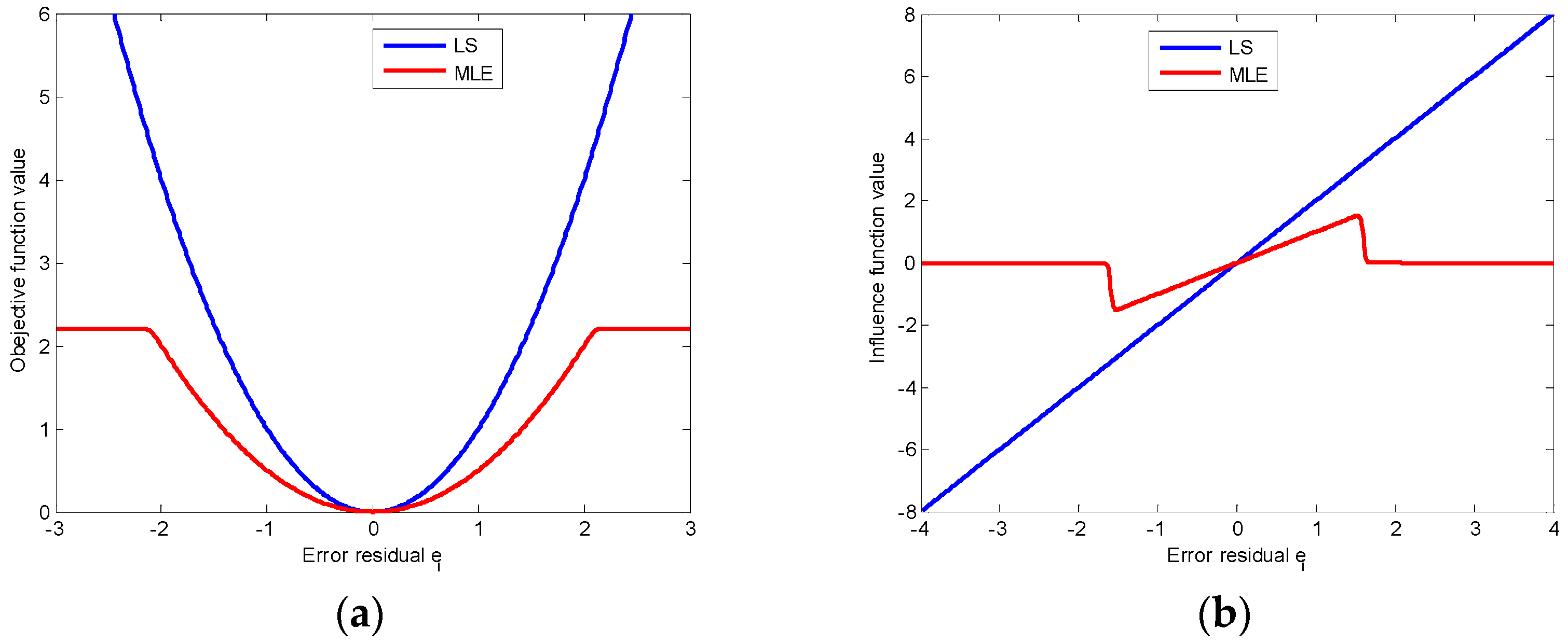
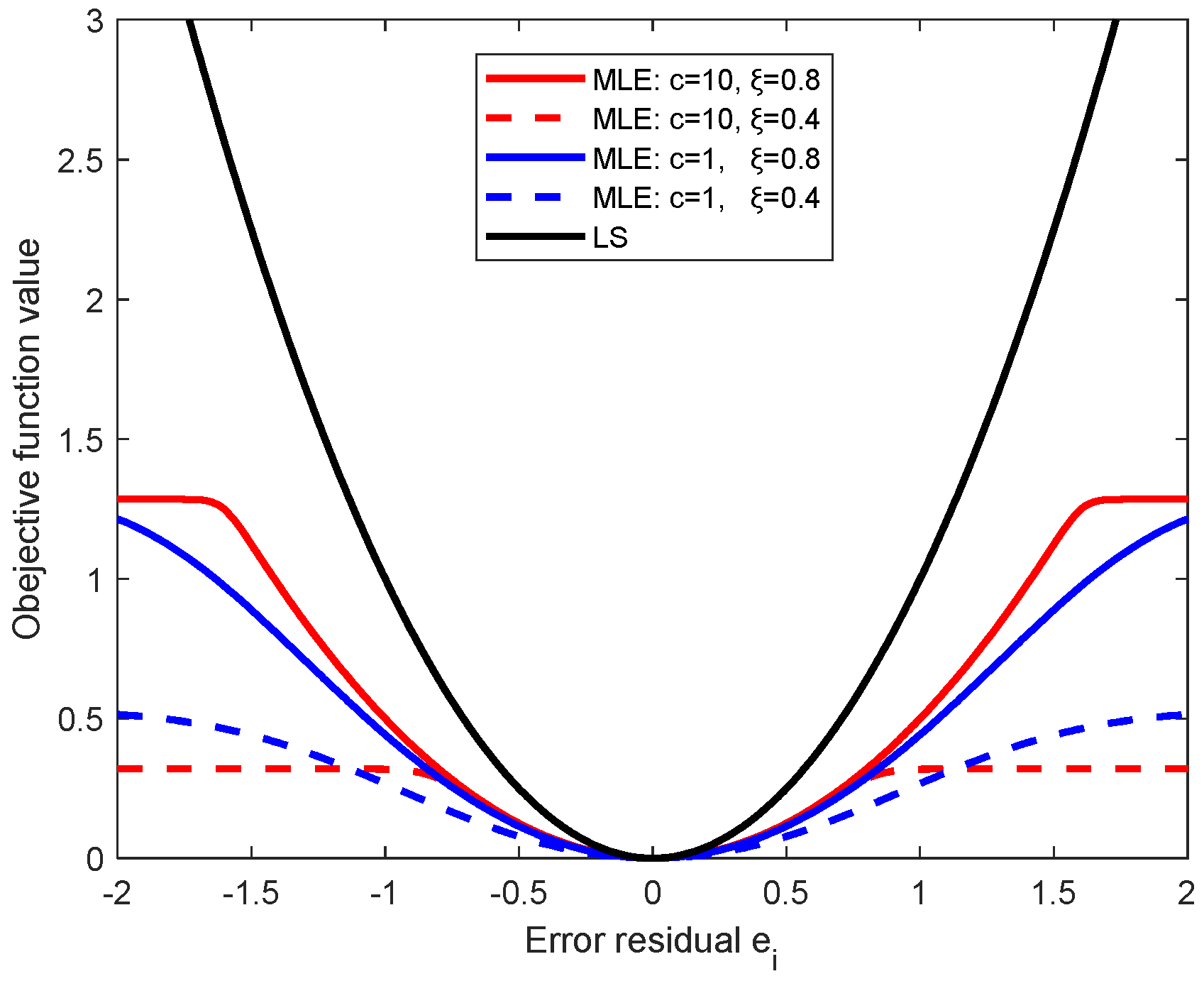
In Figure 2a, we compare the MLE objective function with the LS loss function. MLE objective function is controlled by the parameters $\gamma ,\tau$, and is truncated to a constant for large residuals (e.g., $\left|e_i\right|>2$). As the constant has no effect on the optimization model, the negative effect of noise (points with large residuals) can be automatically diminished. Compared with the MLE function, LS loss function is global and increases quadratically as the increase of residual. When there has heavy noise, the objective function of LS model will be dominated by the points with heavy noise. Figure 2b shows the influence function [22,27] of MLE and LS. The influence function of a loss $\phi \left(e\right)$ is defined as: $\psi \left(e\right)=\partial \phi \left(e\right)/\partial e$, which measures the robustness of loss function as the increase of error residual. For residual $e_i>0$, the influence function of MLE increases first, then decreases and finally reaches the zero value. It means that larger errors finally have no effect on the MLE-based model. However, the influence function of LS continues to grow linearly. So, the LS loss function is seriously affected by noise. In the presence of noise, MLE is obviously more robust than LS.

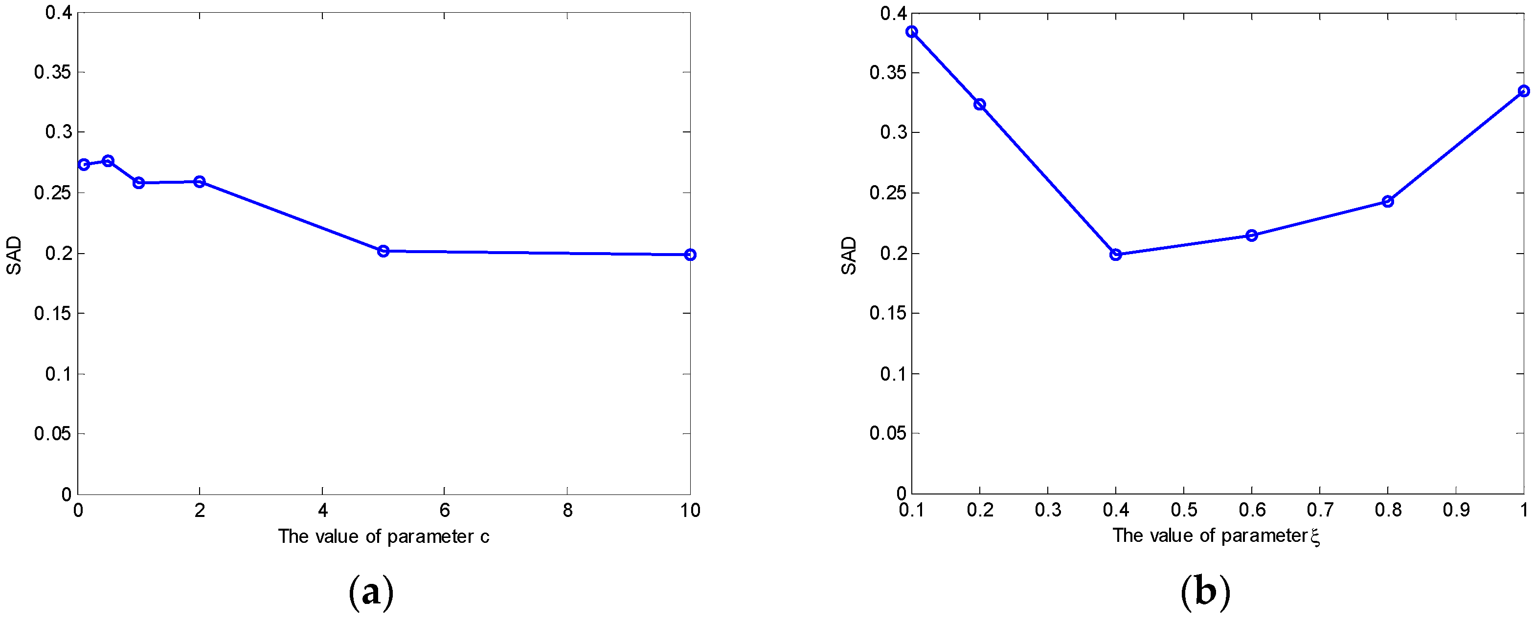
The procedure of the proposed MLENMF is shown in Algorithm 1.

Algorithm 1 MLENMF.

Input: hyperspectral matrix $\mathit{H}$, the parameter $\gamma ,\tau$  Initialization: endmember ${\mathit{Z}}_0$ and abundance ${\mathit{S}}_0$,  Output: estimated endmember and abundance matrices.  1. Initialize ${\mathit{Z}}^{\left(0\right)}={\mathit{Z}}_0, {\mathit{S}}^{\left(0\right)}={\mathit{S}}_0, v=1, \mathit{W}=\mathit{I}$  2. Run the following steps until convergence: (a) Compute the errors: $${\left(e_i^2\right)}^{\left(v\right)}={\Vert {\mathit{H}}^i-{\left({\mathit{Z}}^{\left(v-1\right)}{\mathit{S}}^{\left(v-1\right)}\right)}^i\Vert }_2^2$$ (b) Calculate the weight of each entry: $$w^{\left(v\right)}\left(e_i\right)=\frac{\exp \left(\mathsf{\gamma }\tau -\mathsf{\gamma }{\left(e_i^2\right)}^{\left(v\right)}\right)}{1+\exp \left(\mathsf{\gamma }\tau -\mathsf{\gamma }{\left(e_i^2\right)}^{\left(v\right)}\right)}$$ (c) Compute the weighted matrices: $$\begin{array}{c}\tilde{\mathit{H}}={\left({\mathit{W}}^{\left(v\right)}\right)}^{\frac{1}{2}}\mathit{H}\\ {\tilde{\mathit{Z}}}^{\left(v-1\right)}={\left({\mathit{W}}^{\left(v\right)}\right)}^{\frac{1}{2}}{\mathit{Z}}^{\left(v-1\right)}\end{array}$$ (d) Updating endmember matrix and weighted abundance matrix: $$\begin{array}{c}\left({\tilde{\mathit{Z}}}^{\left(v\right)},{\mathit{S}}^{\left(v\right)}\right)=L_{1/2}\mathrm{NMF}\left(\tilde{\mathit{H}},{\tilde{\mathit{Z}}}^{\left(v-1\right)},{\mathit{S}}^{\left(v-1\right)}\right)\\ {\mathit{Z}}^{\left(v\right)}={\left({\mathit{W}}^{\left(v\right)}\right)}^{-\frac{1}{2}}{\tilde{\mathit{Z}}}^{\left(v\right)}\end{array}$$ (e) $v=v+1$

Remark. 

In the current method, it assumes that different bands are independent and then an MLE solution can be deduced. The band independence assumption is only used in the derivation of MLE estimator. By means of this assumption, it can finally generate a weighted NMF model where the weight function can be used to reduce the effect of noisy bands. Although hyperspectral bands are not independent from each other in practice, the final weighted NMF model (i.e., MLENMF) can still alleviate negative effects of noise.

4. Results

In this section, we perform experiments on a simulated and two real hyperspectral data sets to test the performance of MLENMF model and compare the results with $l_{1/2}$-NMF [13], $l_{21}$-NMF [21], CENMF [19], CIMNMF [18], and HuberNMF (HubNMF for short) [18].

4.1. Evaluation Metrics

Spectral angular distance (SAD) and root mean square error (RMSE) are used to quantitatively evaluate the accuracy of estimated endmembers and abundances.

The formula of SAD is:

$${\mathrm{SAD}}_k=\arccos \left(\frac{{\mathit{z}}_k^T{\widehat{\mathit{z}}}_k}{\Vert {\mathit{z}}_k\Vert ·\Vert {\widehat{\mathit{z}}}_k\Vert }\right),$$

(29)

where ${\mathrm{SAD}}_k$ represents the similarity between the $k$-th real endmember ${\mathit{z}}_k$ and estimated endmember ${\widehat{\mathit{z}}}_k$.

The RMSE is:

$${\mathrm{RMSE}}_k={\left(\frac{1}{N}{\Vert {\mathit{s}}^k-{\widehat{\mathit{s}}}^k\Vert }^2\right)}^{\frac{1}{2}},$$

(30)

where ${\mathit{s}}_k$ and ${\widehat{\mathit{s}}}_k$ are the $k$-th real and estimated abundance maps (i.e., the $k$-th row vector in $\mathit{S}$ and $\widehat{\mathit{S}}$), respectively. $N$ is the number of pixels in HSI.

4.2. Implementation Details

The vertex component analysis (VCA) and fully constrained least squares (FCLS) methods are used to generate the initial endmember $Z_0$ and abundance $S_0$ for different unmixing methods [11,12,13,14,15,16,17,18,19]. The regularization parameter $\mathsf{\lambda }$ in $l_{1/2}$-NMF and CENMF is dependent on the sparsity of the material abundances and is estimated based on the sparseness criterion in Ref. [13]. The parameter of CIMNMF and Huber-NMF are set to be the recommended values in Ref. [18]. The proposed MLENMF contains two parameters $\gamma$ and $\tau$ as shown in Equation (21). It is clear that $\tau$ is related to the amplitude of residual $e_i^2$. For different data sets, the amplitude of residuals may be different. So, it is difficult to determine a specific value of $\tau$. Here, we set $\tau$ in a data-dependent way: $\tau$ is the $\left(100\xi \right)$-th percentile of residual vector $\tilde{\mathit{e}}={\left[e_1^2, \dots , e_M^2\right]}^T$, where $\xi \in \left(0,1\right]$ controls the ratio of inliers. Following Reference [24], parameter $\gamma$ is set as $\gamma =c/\tau$, $c\in \left(0,10\right]$. So, in the experiments, we only need to tune the parameters $\xi$ and $c$.

4.3. Experiments on Simulated Data

Seven spectral signatures (i.e., “Carnallite NMNH98011”, “Actinolite NMNHR16485”, “Andradite WS487”, “Diaspore HS416.3B”, “Erionite+Merlinoit GDS144”, “Halloysite NMNH106236”, “Hypersthene NMNHC2368”) from the USGS spectral library (https://www.usgs.gov/labs/spec-lab, accessed on 2 July 2019) are selected to construct the endmember matrix $\mathit{Z}\in R^{224\times 7}$. Then, these seven spectra are mixed according to the method described in Ref. [28] to form the corresponding abundance matrix $\mathit{S}\in R^{7\times 4096}$. The hyperspectral data matrix is obtained by the product of endmember and abundance matrices, i.e., $\mathit{H}=\mathit{Z}\mathit{S}$. To simulate the real situations, Gaussian noise is added into the data matrix $\mathit{H}$ such that the signal noise ratio (SNR) of different bands follow the Gaussian distribution, i.e., $\mathrm{SNR}~\mathcal{N}\left(\mu ,{\delta }^2\right)$ with $\delta =5$. In the experiment, $\mu \in \left\{5,10,15,20\right\}$ are considered. A large $\mu$ corresponds to small noise. In the MLENMF, parameter $\xi$ is set as 0.4, and parameter $c=10$ is used for $\mu \le 10$ and $c=1$ is used for $\mu \ge 10$.

Table 1. The SAD results of different unmixing methods for simulated data.

$\mathit{\mu }$	NMF	${\mathit{l}}_{1/2}\text{-}\mathbf{NMF}$	${\mathit{l}}_{21}\text{-}\mathbf{NMF}$	CENMF	CIMNMF	HubNMF	MLENMF
5	0.4972	0.4754	0.4324	0.4088	0.4732	0.4718	0.3895
10	0.3513	0.3146	0.2901	0.2813	0.3093	0.3086	0.2537
15	0.1997	0.1749	0.1764	0.1626	0.1781	0.1772	0.1134
20	0.0988	0.0950	0.0936	0.0865	0.0985	0.0946	0.0689

and

Table 2. The RMSE results of different unmixing methods for simulated data.

$\mathit{\mu }$	NMF	${\mathit{l}}_{1/2}\text{-}\mathbf{NMF}$	${\mathit{l}}_{21}\text{-}\mathbf{NMF}$	CENMF	CIMNMF	HubNMF	MLENMF
5	0.2679	0.2763	0.2737	0.2586	0.2653	0.2650	0.2459
10	0.2491	0.2554	0.2497	0.2345	0.2435	0.2448	0.2114
15	0.1951	0.1956	0.1983	0.1811	0.1954	0.1920	0.1440
20	0.1137	0.1219	0.1233	0.1145	0.1208	0.1203	0.0599

show the average results of 20 random experiments under different degrees of noise. Each SAD (RMSE) value is the mean of SAD (RMSE) over seven endmembers. It is clear that the performance of different methods are improved as the increase of SNR or $\mu$, and MLENMF shows better results in different degrees of noise.

To visualize the results of different methods, the real and estimated spectra for the endmember 1 (i.e., “Carnallite NMNH98011”) at $\mu =20$ are shown in Figure 3. Here, we only show the results for the endmember 1 due to space limitations. Similar good results are obtained for the other endmembers. It can be seen that the spectral curve estimated by the MLENMF can well approximate the reference one while the curve of other methods exhibit deviations in amplitude from the reference spectral. As the reference spectral and estimated spectral by different methods have similar shape, the SAD of different methods show small differences as shown in Table 1. Notwithstanding, the estimated abundance map of different methods show large differences as shown in Figure 4. Taking into account both SAD and RMSE results, we can see that our MLENMF method is more robust than other NMF methods when the data contains noise.

4.4. Experiments on Real Data

Two real hyperspectral unmixing data sets, i.e., Urban and Japser are used to evaluate the performance of different NMF unmixing methods (Available at https://rslab.ut.ac.ir/data, https://sites.google.com/site/feiyunzhuhomepage/datasets-ground-truths, accessed on 2 July 2019). The Urban data was obtained by the HYDICE sensor. This scene has the size of $307\times 307$ pixels and each pixel corresponds to an $2\times 2{\mathrm{m}}^2$ area. The original data has 210 bands, where band 1–4, 76, 87, 101–111, 136–153, 198–210 are severely affected by dense water vapor and atmosphere. After removing these noisy bands, 162 bands are kept. This scene contains four reference materials: Asphalt road, Grass, Tree and Roof, which are also available at the https://rslab.ut.ac.ir/data, accessed on 2 July 2019.

We first perform experiments on the Urban data with 162 bands. The parameters of MLENMF are set as: $\xi =0.8$ and $c=1$. The estimated endmembers and abundances by different unmixing methods are compared with the groundtruth references and then the SAD and RMSE results are computed, as shown in

Table 3. The SAD results of different methods for Urban data with 162 bands.

	NMF	${\mathit{l}}_{1/2}\text{-}\mathbf{NMF}$	${\mathit{l}}_{21}\text{-}\mathbf{NMF}$	CENMF	CIMNMF	HubNMF	MLENMF
Asphalt	0.1587	0.1079	0.1576	0.1575	0.1634	0.1601	0.1127
Grass	0.2954	0.2477	0.2983	0.2857	0.2922	0.2826	0.0543
Tree	0.1919	0.1058	0.1917	0.1943	0.1938	0.1923	0.1011
Roof	0.6709	0.5748	0.6841	0.6501	0.6727	0.6534	0.0914
Mean	0.3292	0.2591	0.3329	0.3219	0.3305	0.3221	0.0899

and

Table 4. The RMSE results of different methods for Urban data with 162 bands.

	NMF	${\mathit{l}}_{1/2}\text{-}\mathbf{NMF}$	${\mathit{l}}_{21}\text{-}\mathbf{NMF}$	CENMF	CIMNMF	HubNMF	MLENMF
Asphalt	0.2126	0.2843	0.2123	0.2114	0.2126	0.2127	0.1383
Grass	0.2386	0.2683	0.2395	0.2391	0.2394	0.2385	0.1318
Tree	0.1692	0.1387	0.1693	0.1699	0.1693	0.1691	0.0605
Roof	0.1574	0.1718	0.1568	0.1574	0.1569	0.1574	0.0538
Mean	0.1945	0.2158	0.1945	0.1945	0.1945	0.1944	0.0961

, respectively. Compared with other NMF methods, the proposed MLENMF shows better overall results. Figure 5 shows the estimated endmembers by different methods. It can be seen that the other methods cannot well estimate the endmember ‘Roof’, while our MLENMF generates spectral curve that is similar to the reference signature. From the abundance maps in Figure 6, we can see that the maps of MLENMF are more consistent with the reference maps than comparison methods.

To test the unmixing performance of different methods in the case of noisy bands, we also calculate the SAD and RMSE for the Urban data with the whole 210 bands and show the results in

Table 5. The SAD results of different methods for Urban data with 210 bands.

	NMF	${\mathit{l}}_{1/2}\text{-}\mathbf{NMF}$	${\mathit{l}}_{21}\text{-}\mathbf{NMF}$	CENMF	CIMNMF	HubNMF	MLENMF
Asphalt	0.1229	0.1234	0.1295	0.1271	0.1345	0.1312	0.1481
Grass	0.4703	0.3544	0.4607	0.4854	0.4637	0.4618	0.1436
Tree	0.3197	0.2057	0.3139	0.3401	0.3035	0.3048	0.1979
Roof	0.4446	0.3048	0.4083	0.4705	0.4466	0.4348	0.3039
Mean	0.3394	0.2471	0.3281	0.3558	0.3371	0.3332	0.1984

and

Table 6. The RMSE results of different methods for Urban data with 210 bands.

	NMF	${\mathit{l}}_{1/2}\text{-}\mathbf{NMF}$	${\mathit{l}}_{21}\text{-}\mathbf{NMF}$	CENMF	CIMNMF	HubNMF	MLENMF
Asphalt	0.2443	0.3204	0.2453	0.2391	0.2428	0.2441	0.2659
Grass	0.3763	0.4655	0.3770	0.3761	0.3770	0.3769	0.2985
Tree	0.3374	0.3711	0.3381	0.3373	0.3380	0.3380	0.2679
Roof	0.2213	0.2377	0.2217	0.2155	0.2197	0.2208	0.2616
Mean	0.2948	0.3487	0.2955	0.2920	0.2944	0.2949	0.2735

, respectively. The parameters of MLENMF in this case are set as: $\xi =0.4$ and $c=10$. Even with some known bad bands, our MLENMF also provides the best results.

The Japser data is collected by the AVIRIS sensor, covering a spectral range of 380 to 2500 nm, with a total of 224 spectral bands, including 26 noisy bands. The spectral resolution is 9.46 nm, and the image size is 100 × 100. The image mainly contains four materials: Tree, Water, Soil, and Road. The parameters of MLENMF are set as: $\xi =0.4$ and $c=1$. The SAD and RMSE results of different unmixing methods on this data set are shown in

Table 7. The SAD results of different methods for Jasper data.

	NMF	${\mathit{l}}_{1/2}\text{-}\mathbf{NMF}$	${\mathit{l}}_{21}\text{-}\mathbf{NMF}$	CENMF	CIMNMF	HubNMF	MLENMF
Tree	0.3040	0.2787	0.2981	0.2503	0.2189	0.3029	0.0851
Water	0.3156	0.1163	0.2799	0.2974	0.2968	0.2969	0.1841
Soil	0.2834	0.1660	0.3186	0.3871	0.2490	0.1872	0.0908
Road	0.6469	0.5341	0.6627	0.6953	0.7052	0.6961	0.2269
Mean	0.3875	0.2738	0.3898	0.4075	0.3675	0.3708	0.1468

and

Table 8. The RMSE results of different methods for Jasper data.

	NMF	${\mathit{l}}_{1/2}\text{-}\mathbf{NMF}$	${\mathit{l}}_{21}\text{-}\mathbf{NMF}$	CENMF	CIMNMF	HubNMF	MLENMF
Tree	0.2310	0.3032	0.2711	0.2251	0.2287	0.2350	0.1055
Water	0.1563	0.1726	0.1738	0.1623	0.1502	0.1508	0.1029
Soil	0.3382	0.3789	0.3342	0.3209	0.3045	0.3207	0.2510
Road	0.2385	0.2634	0.2534	0.2639	0.2351	0.2337	0.2350
Mean	0.2410	0.2796	0.2581	0.2430	0.2296	0.2351	0.1736

, respectively. Figure 7 and Figure 8 show the estimated endmembers and abundance maps of different methods. It can be seen from these results that the proposed MLENMF can provide more accurate estimation on the endmembers and abundances.

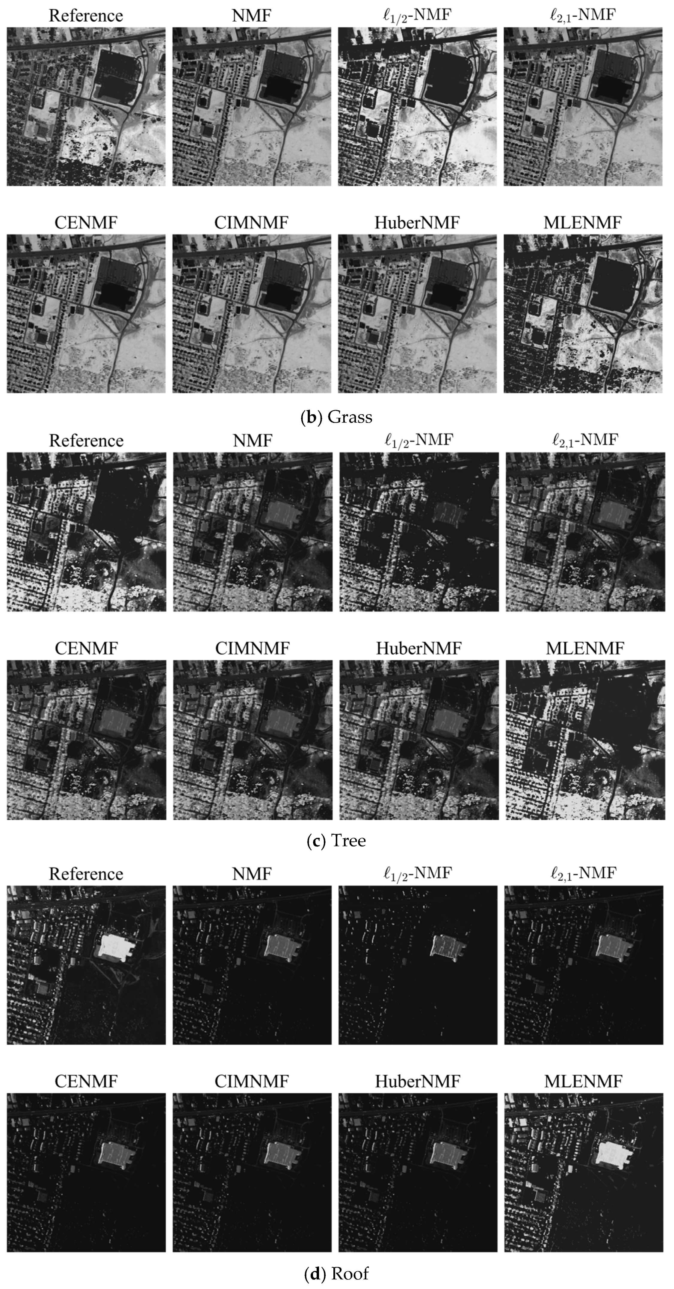
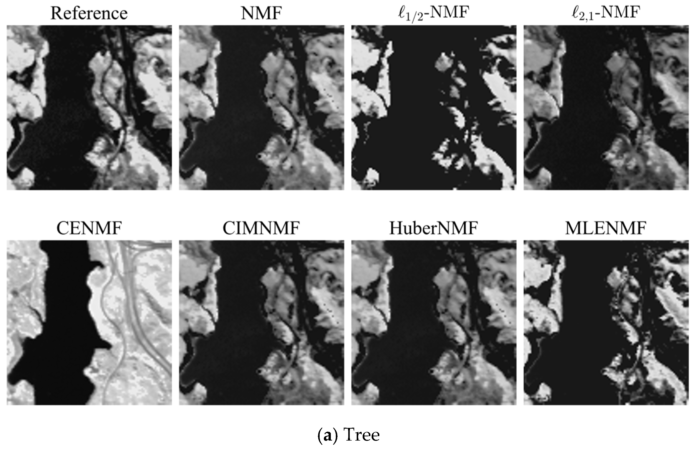
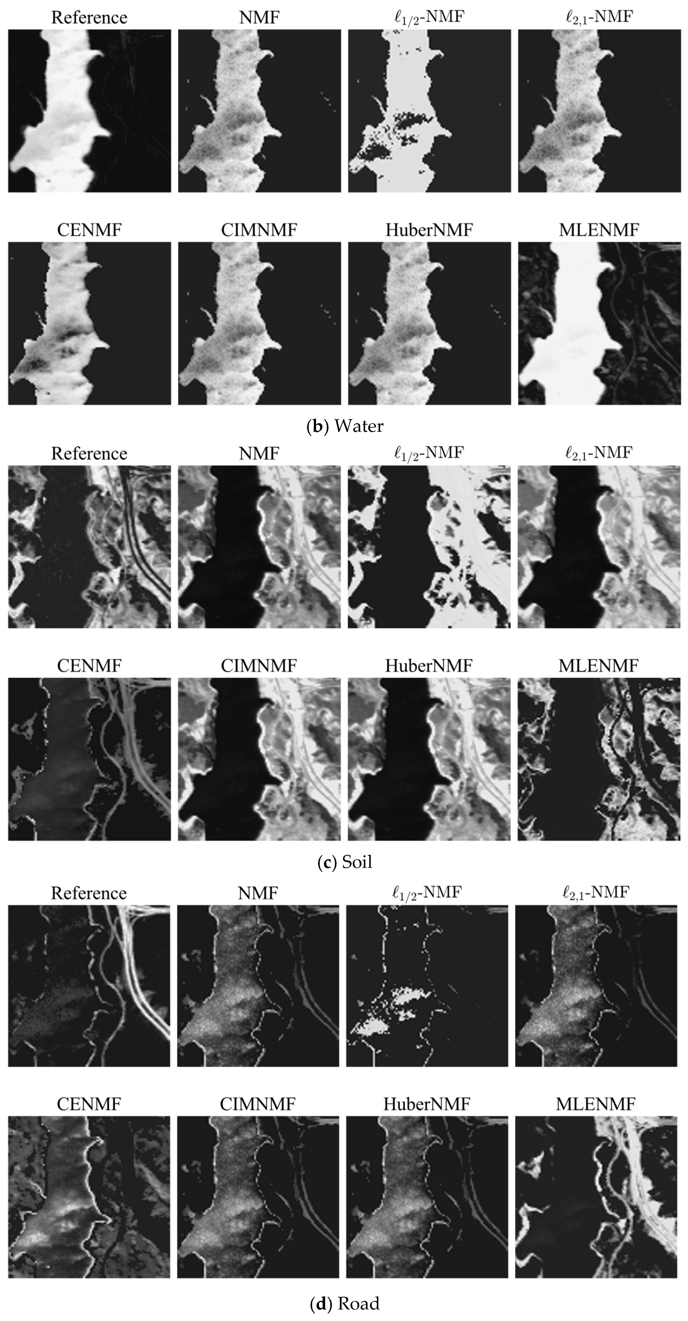
5. Discussion

As described in Section 4.2, $\tau$ is the $\left(100\xi \right)$-th percentile of residual vector $\tilde{e}={\left[e_1^2, \dots , e_M^2\right]}^T$, and $\gamma =c/\tau$, $c\in \left(0,10\right],\xi \in \left(0,1\right]$. By tuning the parameters $c$ and $\xi$, the MLE objective function in Equation (26) can be truncated, as shown in Figure 9. Parameter $c$ and $\xi$ control the decreasing rate and the location of truncation point, respectively. The larger the value of $c$, the greater the degree of truncation. The smaller the value of $\xi$, the more forward the position of the truncation point. As shown in Figure 9, when the noise or residual is large, it is better to choose a larger $c$ and a smaller $\xi$ that truncates the weight of larger residuals to a constant (seeing the red dotted line).

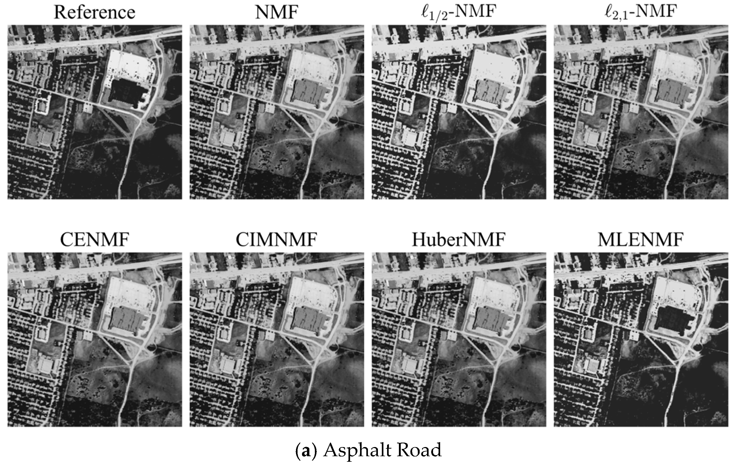
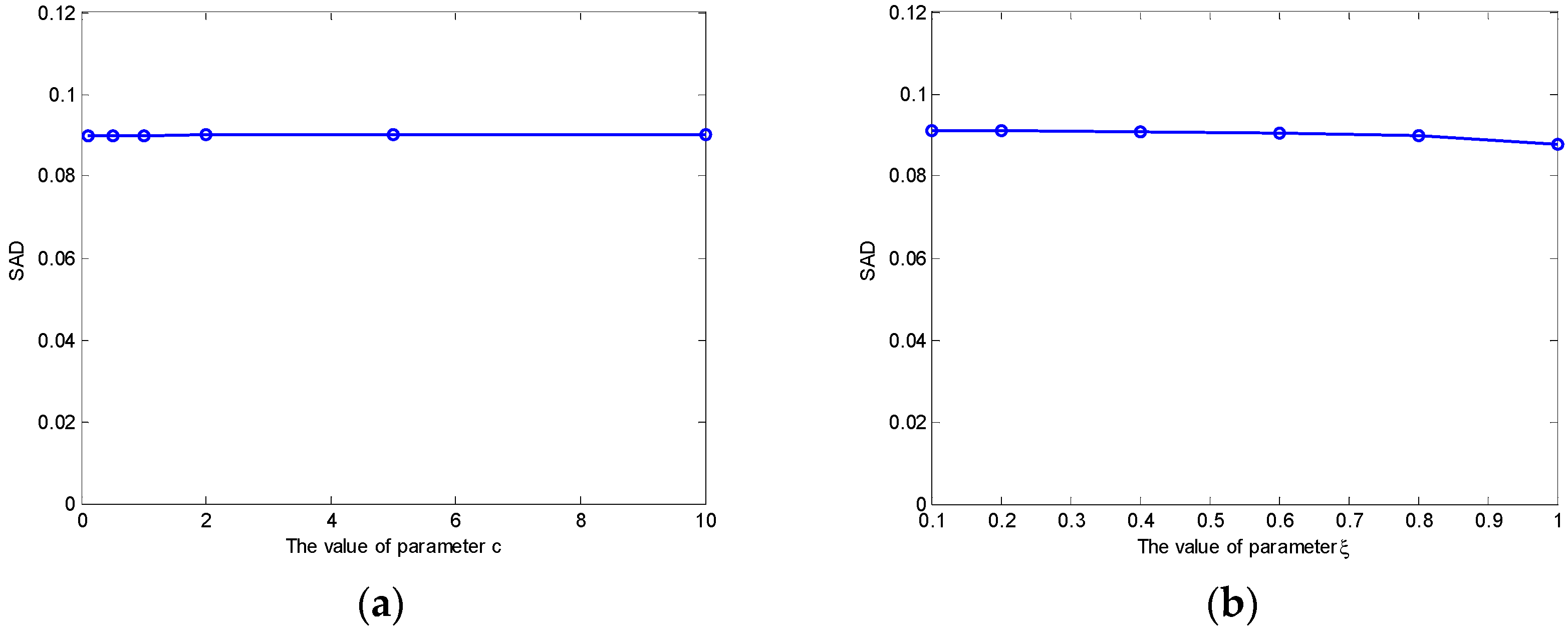
We take the Urban data set as an example to show the effect of parameters $c$ and $\xi$. Figure 10 shows the SAD results of MLENMF on Urban data with 210 bands. The results in Figure 10a are obtained by fixing $\xi =0.4$ and changing $c$ in the set $\left\{0.1,0,5,1,2,5,10\right\}$. When $\xi$ is fixed, larger $c$ values correspond to better unmixing results. As shown in Figure 9, $c$ affects the degree of truncation. If choosing a large $c$, the weight of large errors can be truncated to a constant (e.g., the objective function values are constant for errors larger than 1.5, showing as the red solid line in Figure 9). As their objective function values are constant, they have no influence on the model. For Urban data with all 210 bands, MLENMF with a larger $c$ can effectively alleviate the effect of noisy bands. By fixing $c=10$ and changing $\xi$ in the set $\left\{0.1,0.2,0,4,0.6,0.8,1\right\}$, Figure 10b shows the SAD of MLENMF versus parameter $\xi$. It is better to set the parameter $\xi$ in the interval [0.4 0.8] when $c$ is fixed. Parameter $\xi$ determines the ratio of inliers. As the data contains noisy bands, the value of $\xi$ should be less than 1.

When the known noisy bands on the Urban data are removed, the experimental results on Urban data with 162 bands are obtained at fixing $\xi =0.8$ and $c=1$, respectively. The results are shown in Figure 11. From Figure 11a, we can see that the proposed MLENMF is not sensitive to parameter $c$ because different $c$ values generate similar results for small errors in the case of low noise or no noise data as shown in Figure 9. From Figure 11b, the best result is achieved at $\xi =1$, which means that the data points are almost inliers.

The above analysis recommends setting the parameter $\xi$ in the interval [0.4 0.8]. For data with heavy noise, $\xi$ can be set to be a small value, such as $\xi =0.4$. Parameter $c$ is chosen in the interval [1,10]. For data with heavy noise, it can set $c=10$. Otherwise, a moderate value $c=1$ is recommended.

6. Conclusions

This paper proposes a maximum likelihood estimation-based nonnegative matrix factorization (MLENMF) model for hyperspectral unmixing. The proposed MLENMF employs an MLE-like loss function that replaces the least-squares loss function in the NMF model. The MLE-like loss is a robust loss, which can truncate the objective function value of noise and can reduce their negative effects on the unmixing model. Experimental results on a simulated data and two real data sets (Urban and Jasper) show that the proposed MLENMF model has obvious noise suppression effect and can obtain more accurate unmixing results. In the current model, it assumes that different bands are independent and then an MLE solution can be deduced. Notwithstanding, in practice the assumption of band independence is not generally valid. Taking also into account the dependence between different bands, improved the unmixing performance may result. However, this issue deserves further research. In addition, parameter selection is a key problem for the unmixing model. The cross-validation strategy can be considered for parameter selecting, such as dividing the whole hyperspectral image into two disjoint subimages, one for training and another for testing, and then performing cross-validation to automatically select the parameters. This also deserves research in the future.