Article

Vision Transformers for Remote Sensing Image Classification

1
Computer Engineering Department, College of Computer and Information Sciences, King Saud University, Riyadh 11543, Saudi Arabia
2
Applied Computer Science Department, College of Applied Computer Science, King Saud University, Riyadh 11543, Saudi Arabia
*
Author to whom correspondence should be addressed.
Remote Sens. 2021, 13(3), 516; https://doi.org/10.3390/rs13030516
Submission received: 23 December 2020 / Revised: 21 January 2021 / Accepted: 29 January 2021 / Published: 1 February 2021

Abstract

:
In this paper, we propose a remote-sensing scene-classification method based on vision transformers. These types of networks, which are now recognized as state-of-the-art models in natural language processing, do not rely on convolution layers as in standard convolutional neural networks (CNNs). Instead, they use multihead attention mechanisms as the main building block to derive long-range contextual relation between pixels in images. In a first step, the images under analysis are divided into patches, then converted to sequence by flattening and embedding. To keep information about the position, embedding position is added to these patches. Then, the resulting sequence is fed to several multihead attention layers for generating the final representation. At the classification stage, the first token sequence is fed to a softmax classification layer. To boost the classification performance, we explore several data augmentation strategies to generate additional data for training. Moreover, we show experimentally that we can compress the network by pruning half of the layers while keeping competing classification accuracies. Experimental results conducted on different remote-sensing image datasets demonstrate the promising capability of the model compared to state-of-the-art methods. Specifically, Vision Transformer obtains an average classification accuracy of 98.49%, 95.86%, 95.56% and 93.83% on Merced, AID, Optimal31 and NWPU datasets, respectively. While the compressed version obtained by removing half of the multihead attention layers yields 97.90%, 94.27%, 95.30% and 93.05%, respectively.

1. Introduction

Remote sensing (RS) is the science of collecting information about objects without any direct physical contact, typically through a satellite, aircraft or unmanned aerial vehicle (UAV) [1]. Examples of applications of remote sensing include geological survey, environment testing, oil exploration, traffic management, earthquake prediction, and water conservancy construction [2,3].
Remote-sensing images have improved in both spatial and temporal resolutions with the evolution of satellite sensors, which provides opportunities in resolving fine details on the earth’s surface. Satellites such as MODIS (1 km × 1 km) offering thermal data with high temporal resolution suffer from low spatial resolution. Landsat, on the other hand, offers small-scale variations of 100–200 m but with very low temporal resolution. The new generation of satellites can deliver very high spectral and spatial images; for example, IKONOS-2 generates images with 4-band multispectral resolution and spatial resolution from 2.5 to 4 m. Unmanned aerial vehicles (UAVs) present an improved solution of remote-sensing acquisition platforms, which witnessed a high level of growth in past years and are used widely for fire detection, surveillance mapping, and landslide monitoring, among other uses [4]. UAVs have several advantages over satellite and aerial images. First, they are easier to deploy to satisfy the requirements of rapid monitoring, assessment, and mapping. They can work at lower altitudes compared to the piloted aircraft, which provides spatial resolution at the centimeters level. They can fly any time the weather permits, leading to improvements in temporal resolution. As the spatial resolution increases, images are likely to contain noisy and outlying descriptors. A recent study [5] proposed a convolutional neural network (CNN) to classify images captured by a camera mounted on a UAV. Al-Najjar et al. [6] proposed a CNN model to classify a digital surface model beside UAV images. Liu et al. [7] combined CNNs with object-based image analysis (OBIA) for land cover classification using multiview data. The author in [8] proposed a two-branch neural network to assign multiple class labels to UAV imagery.
The topic of scene classification has been an active research field lately to face the challenging problem of effectively interpreting remote-sensing images. It is the task of taking an image and correctly labeling it to a predefined class as shown in Figure 1. Scene classification is an important task for many applications, such as land management [9], urban planning [10], and modeling wildfires [11].
The early works on scene classification were based on handcrafted features, manually extracted by humans, including local binary patterns (LBP) [12], histogram of oriented gradients (HOG) [13], and the scale-invariant feature transform (SIFT) [14]. Conventional scene-classification methods depend on encoding handcrafted features with different models such as the bag-of-words (BoWs) [15], Fisher vectors (FV) [16], or the vector of locally aggregated descriptors (VLAD) [17].
On the other hand, deep learning methods such as Deep Belief Networks (DBNs) [18] and stacked auto-encoders [19] gained enormous achievements in several applications, including remote-sensing image classification. In particular, CNNs have surpassed traditional methods in many applications [20,21,22]. These methods have a main key advantage of providing an end-to-end solution, which requires minimal feature engineering. Other approaches based on recurrent neural networks (RNNs) [23], generative adversarial networks (GANs) [24,25], graph convolutional networks (GCNs) [26], and long- short-term memory (LSTM) [27] have been introduced also. In a recent contribution, the authors considered remote-sensing scene classification as a multiple-instance learning (MIL) problem [28]. They proposed a multiple-instance densely connected network to highlight the local semantics relevant to the scene label. The method enhances the capability of local semantic representation by effectively discarding useless information. Yu et al. [29] proposed the attention GAN, which integrates GANs with the attention mechanism to enhance the representation power of the discriminator for aerial scene classification. The authors in [30] introduced a simple fine-tuning method using an auxiliary classification loss. They showed how to combat the vanishing gradient problem using an auxiliary loss function. Sun et al. [31] proposed a gated bidirectional network for feature fusion. Liu et al. [32] combined the feature maps from intermediate and fully connected layers and input them to the classifier for classification. Yu et al. [33] combined two pretrained CNNs with the two-stream fusion technique to classify high-resolution aerial scenes. Cheng et al. [34] proposed a metric learning regularization on discriminative CNNs features to optimize a new discriminative objective function to make the model more discriminative. Xue et al. [35] proposed a method using three deep networks to extract deep features from the image separately. Then these features were fused together to create a single feature vector for classification.
Besides CNNs, a new type of deep-learning models called Transformers have been proposed and received some popularity in computer vision. Transformers rely on a simple but powerful procedure called attention, which focuses on certain parts of the input to get more efficient results. Currently, they are considered state-of-the-art models in sequential data, in particular natural language processing (NLP) methods such as machine translation [36], language modeling [37], and speech recognition [38]. The architecture of the Transformer developed by Vaswani et al. [39] is based on the encoder–decoder model, which transforms a given sequence of elements into another sequence. The main motivation for transformers was to enable parallel processing of the words in a sentence, which was not possible in LSTMs or RNNs because they take words of a sentence one by one.
Inspired by the success of Transformers in NLP, new research tries to apply Transformers directly to images. This is a challenging task, due to the need in self-attention application that every pixel attends to all other pixels. For images, this is very costly because the image contains a huge number of pixels. Researchers tried several approaches to apply Transformers to images. Some works combined CNN architectures with self-attention. For example, Bello et al. [40] enhanced CNNs by replacing some convolutional layers with self-attention layers, which led to improvement in image classification. However, this method faced high computational cost because the large size of the image causes an enormous growth in the time complexity of self-attention. Wang et al. [41] proposed a method to generate powerful features by selectively focusing on critical parts or locations of the image, then processing them sequentially. Wu et al. [42] used the Transformer on top of the CNN; first they extracted feature maps using a CNN, then fed them to stacked visual Transformers to process visual tokens and compute the output. Ramachandran et al. [43] first started to use self-attention as a stand-alone building block for vision tasks instead of a simple augmentation on top of convolutional layers. They set up a fully attention model by replacing all convolutional layers with self-attention layers. Chen et al. [44] proposed a method that applies Transformers to raw images with reduced resolution and reshaped into textlike long sequences of pixels.
In a very recent contribution, and different from previous works, Dosovitskiy et al. [45] applied a standard Transformer directly to images by splitting the image into patches not focusing on pixels, then input to the Transformer the sequence of embeddings for those patches. The image patches were treated as tokens in NLP applications. These models led to very competitive results on the ImageNet dataset. In this work, we will exploit these pretrained models for transferring knowledge to the case of remote-sensing imagery. Indeed, to the best of our knowledge in remote-sensing scene-classification tasks, convolutional architectures remain dominant and Transformers have not yet been widely used as the model choice in classification. For instance, He et al. [46] proposed a model derived from the bidirectional encoder representations called BERT [47] that was used in the natural language processing field to the context of hyperspectral images. The method is based on several multihead self-attention layers. Each head encodes the semantic context-aware representation to obtain discriminative features that are needed for accurate pixel-level classification.
In this paper, we propose an extensive evaluation of the model proposed in [45] for the classification of remote-sensing images. To this end, the images under analysis are divided into patches, then converted to sequence by flattening and embedding. The position embedding is added to these patches to keep the position information. The obtained sequence is then fed to several multihead attention layers for generating the final representation. During classification, the first token sequence is fed as input to a softmax classification layer. To increase the classification performance, we explore several data augmentation strategies such as CutMix, and Cutout to generate additional data for training. In the experiments, we show that we can compress the network by pruning half of its layers while keeping competing classification accuracies.
The remainder of the paper is organized as follows: Section 2 describes the main methods based on Transformers. In Section 3, we present the experimental results on three well-known datasets. Section 4 provides a discussion about the results and presents comparisons with state-of-the-art methods. Then we finally conclude and show future directions in Section 5.

2. Materials and Methods

2.1. Vision Transformer

Let S = X i ,   y i i = 1 r donate a set of r remote sensing images, where   X i is an image and y i is its corresponding class label y i 1 ,   2 ,   , m , and m is the number of defined classes for that set. The objective of the Vision Transformer model is to learn the mapping from the sequence of image patches to the corresponding semantic label.
Vision Transformer is an architecture that is based entirely on the vanilla Transformer [39], the architecture that has attracted a lot of interest in recent years by showing state-of-the-art performance in machine translation and other NLP tasks [47]. The Transformer follows the encoder–decoder architecture, with the ability to process sequential data in parallel without relying on any recurrent network. The success of Transformer models has largely benefited from the self-attention mechanism, which is proposed to capture long-range relationships between the sequence’s elements.
Vision Transformer is proposed as an attempt to extend the use of the standard Transformer to image classification. The main goal is to generalize them on modalities other than text without integrating any data-specific architecture. In particular, Vision Transformer utilizes the encoder module of the Transformer to perform classification by mapping a sequence of image patches to the semantic label. Unlike the conventional CNN architectures that typically use filters with a local receptive field, the attention mechanism employed by the Vision Transformer allows it to attend over different regions of the image and integrate information across the entire image.
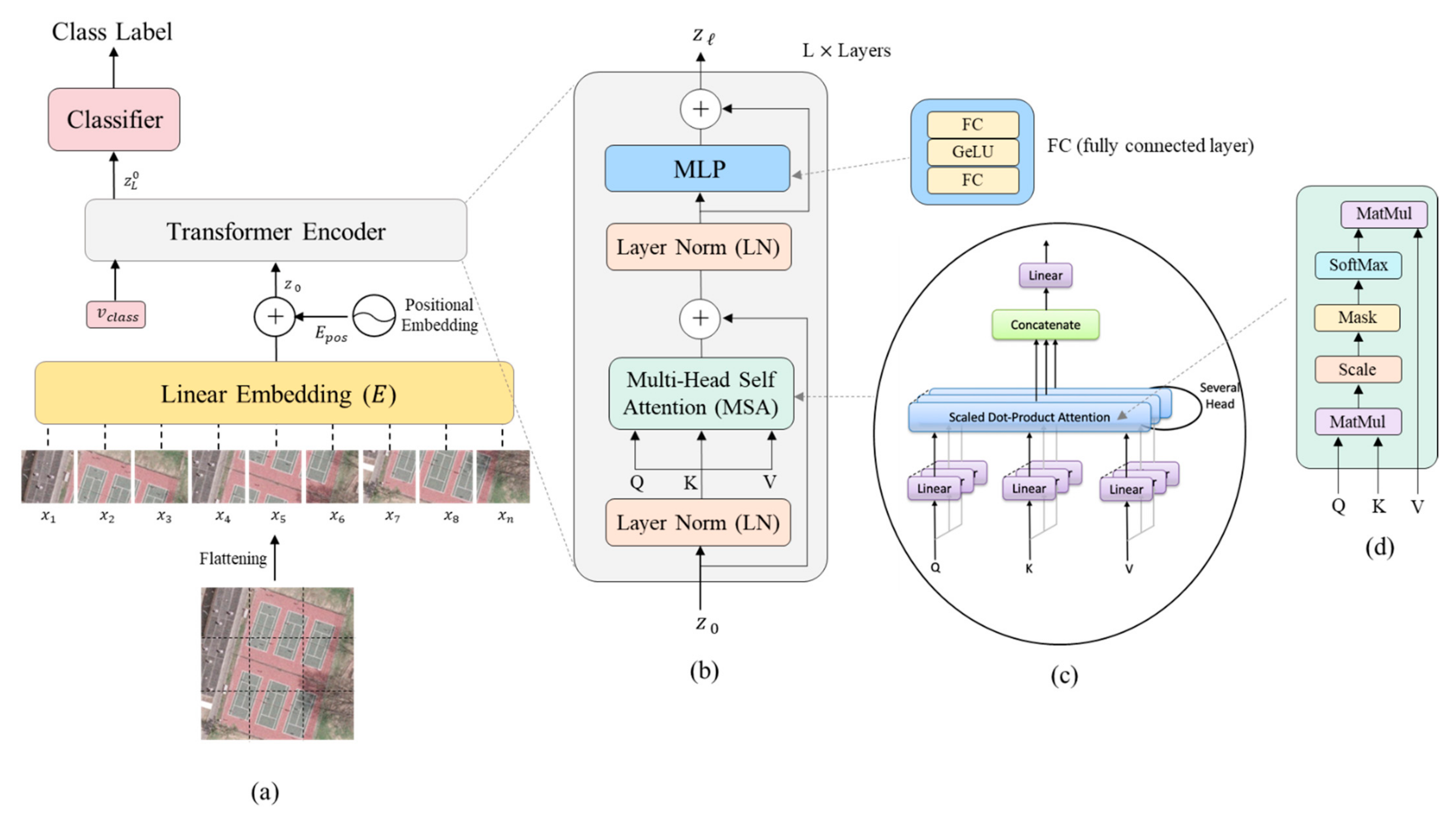
The complete end-to-end architecture of the model is shown in Figure 2. In general, it is composed of an embedding layer, an encoder, and a final head classifier. In the first step, an image X from the training set (for simplicity, we omit the image index i ) is subdivided into non-overlapping patches. Each patch is viewed by the Transformer as an individual token. Thus for an image of X size c × h × w (where   h is the height, w is the width and c represents the number of channels), we extract patches each of dimension c × p × p from it. This forms a sequence of patches x 1 , x 2 , , x n of length n , with n = h w / p 2 . Typically, the patch size p is chosen as 16 × 16 or 32 × 32 , where a smaller patch size results in a longer sequence and vice versa.

2.1.1. Linear Embedding Layer

Before feeding the sequence of patches into the encoder, it is linearly projected into a vector of the model dimension d using a learned embedding matrix   E . The embedded representations are then concatenated together along with a learnable classification token v c l a s s that is required to perform the classification task. The embedded image patches are viewed by the Transformer as a set of patches without any notion of their order. To keep the spatial arrangement of the patches as in the original image, the positional information E p o s is encoded and appended to the patch representations. The resulting embedded sequence of patches with the token z 0 is given in (Equation (1)):
z 0 = v c l a s s ;   x 1 E ; x 2 E ; ;   x n E + E p o s ,   E p 2 c × d ,   E p o s n + 1 × d
It has been shown in [45], that 1-D and 2-D positional encodings produce nearly identical results. Therefore, a simple 1-D positional encoding is used to preserve the positional information of the flattened patches.

2.1.2. Vision Transformer Encoder

The resulting sequence of embedded patches z 0   is passed to the Transformer encoder. As shown in Figure 2b, the encoder is composed of L identical layers. Each one has two main subcomponents: (1) a multihead self-attention block (MSA) (Equation (2)), and (2) a fully connected feed-forward dense block (MLP) (Equation (3)); the latter block consists of two dense layers with a GeLU activation in between. Each of the two subcomponents of the encoder employs residual skip connections and is preceded by a normalization layer ( LN ) .
z = MSA LN z 1 +   z 1 ,     = 1 L
z = MLP LN z +   z ,     = 1 L
At the last layer of the encoder, we take the first element in the sequence z L 0 and pass it to an external head classifier for predicting the class label.
y = LN z L 0
The MSA block in the encoder is the central component of the Transformer. It has the role of determining the relative importance of a single patch embedding with respect to the other embeddings in the sequence. This block has four layers: the linear layer, the self-attention layer, the concatenation layer, which concatenates the outputs of the multiple attention heads, and a final linear layer, as shown in Figure 2c.
At a high level, attention can be represented by attention weight, which is computed by finding the weighted sum over all values of the sequence z . The self-attention (SA) head learns the attention weights by computing the query-key-value scaling dot-product. Figure 2d shows the details of the computation that takes place in the SA block. For each element in the input sequence, three values are generated: Q (query), K (key), and V (value) by multiplying the element against three learned matrices U Q K V   (Equation (5)). To determine the relevance between an element with other elements on the sequence, the dot product is calculated between the Q vector of this element with the K vectors of other elements. The results determine the relative importance of patches in the sequence. The results of the dot-product are then scaled and fed into a softmax (Equation (6)). The scaling dot-product operation performed by the SA block is similar to the standard dot-product, but it incorporates the dimension of the key D K as a scaling factor. Finally, the value of each patch embedding’s vector is multiplied by the output of the softmax to find the patch with the high attention scores (Equation (6)). The full operation is given by these equations:
Q ,   K , V = z U Q K V ,   U Q K V d × 3 D K
A = softmax Q K T D K ,     A n × n
SA z = A . V
The MSA block computes the scaled dot-product attention separately for h heads using the previous operation, but instead of using a single value for the Query, Key, and Value, multiple values are used. The results of all of the attention heads are concatenated together and then projected through a feed-forward layer with learnable weights W to the desired dimension. This operation is expressed by this equation:
MSA ( z ) = Concat SA 1 z ;   SA 2 z ;   SA h z W ,         W h . D K × D

2.1.3. Vision Transformer Variants

To experiment on the effect of increasing the model size on the classification accuracy, different versions of Vision Transformer have been proposed in [45]: the “ViT-Base”, the “ViT-Large”, and the “ViT-Huge”. The three versions differ in the number of the encoder’s layers, the hidden dimension size, the number of attention heads used by MSA layer, and the MLP classifier size. Each one of these models is trained with a patch of size 16 × 16 and 32 × 32 . The “ViT-Base” model has 12 layers in the encoder, with hidden size 768, and uses 12 heads in the attention layer. The other version uses larger numbers; the “ViT-Large” for example, has 24 layers, 16 attention heads, and a hidden dimension of size 1024. The “ViT-Huge” has 32 layers, 16 attention heads, and a hidden size of 1280. Table 1 shows a comparative summary of the Transformer versions.
The experimental results on Vision Transformers of different size have shown that using relatively deeper models is important to get higher accuracy. Moreover, choosing a small patch dimension increases the sequence length n , which in turn improves the overall accuracy of the model. Another important finding is that attention heads at the earlier layers of the Vision Transformer can attend image regions at high distances. This ability increases as the depth of the model increases. This is different from the CNNs-based models, in which earlier layers can only detect local information and global information can only be detected at the higher layers of the network. This property of the Vision Transformer is crucial for detecting the relevant features for classification.

2.2. Data Augmentation Strategies

Data augmentation is a simple but effective tool for increasing the size and diversity of the training dataset. It is a fundamental step for tasks where the access to a large annotated dataset is not feasible [48]. Data augmentation uses different manipulation techniques to generate additional training samples from the existing one while preserving the validity of the original class label. Training a model on augmented data helps to combat the overfitting problem and thus improve the robustness and the generalization ability of the model.
Standard data augmentation techniques create new samples by applying simple geometric transformations such as rotating, scaling, cropping, shifting, and flipping, or use a combination of them. Color-space augmentation strategies expand the dataset by applying transformations on the color space such as adjusting the brightness, the contrast, or the color saturation of the images. Neural style transfer [49] extends the transformations to include the low-level features of the image, such as texture. It transfers the style of one image in the dataset to another image while keeping its semantic content. One interesting approach for data augmentation is the one based on generative models, in which models such as GANs [50] learn the distribution of the data to create synthetic samples that are as similar as possible to the images drawn from the original dataset.
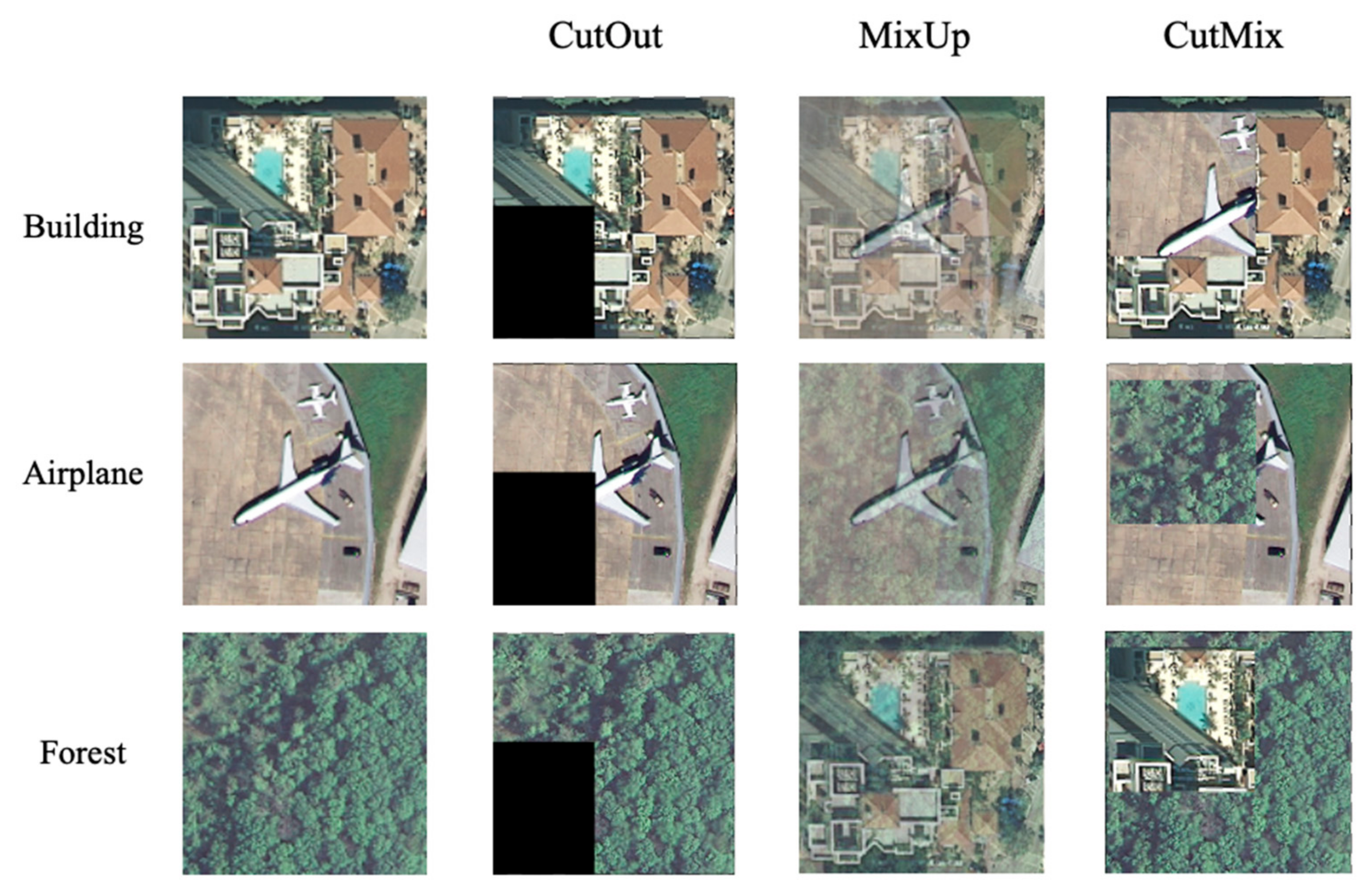
More sophisticated techniques based on random erasing and image-mixing have been introduced recently to generate more challenging samples for the model such as Cutout [51], Mixup [52], and CutMix [53] techniques. In Cutout, a random fixed-size region of the image is intentionally replaced with black pixels or random noise. This technique was developed to tackle the problem of occluded objects in scene classification and object detection. A randomly chosen region is erased to encourage the model to learn from the entire image’s context rather than relying on a specific visual feature. One problem of using Cutout is that blocking could hide an essential part of the object, causing information loss [53]. CutMix technique overcomes this problem by cutting a patch of one image and replacing it with a patch from another image in the dataset. This can mitigate the information loss of the Cutout technique.
With Mixup, two images are merged by linearly interpolating them along with their class labels to create a new training instance. For both the CutMix and the Mixup augmentation, the ground truth label is changed in accordance with the changes applied to the image. If X i , y i and X j , y j are two samples drawn randomly from the training data and λ 0 ,   1 . The mixup augmentation expands the dataset by interpolating the two samples X i and X j   and their associated one-hot label encodings y i and y j using the following equations:
X ¯ =   λ X i + 1 λ X j
y ¯ =   λ y i + 1 λ y j
Figure 3 shows examples of applying Cutout, Mixup, and CutMix on Merced dataset. Choosing the best strategy to apply for data augmentation is usually a manual process. Advanced methods of data augmentation try to automate the search for the optimal transformation for the target task, without the need for any human intervention [48].

2.3. Network Compression

Transformers have a deep and rich architecture with millions of parameters, hundreds of attention heads and multiple layers. As can be seen in Table 1, the ViT-Base model, for example, has more than 80 million parameters. In general, models with large architecture tend to produce better results. However, the enormous computational complexity and the huge memory requirement associated with these models make them impractical for deployment and prone to overfitting.
Model-compression techniques aim at producing a lighter version of the model without hurting the original accuracy. Knowledge distillation and model pruning are commonly used compression approaches. With knowledge distillation, the information encoded in a well-trained model usually named as the teacher model is transferred to another smaller model known as the student model [54]. The student network supervised by the teacher network gradually learns how to produce results that are consistent with the results provided by the teacher network. Model pruning [55] is another technique that is used for compression. It tries to decrease the number of the model’s parameters by removing redundant or inessential components, keeping only the important components. Pruning can take several forms, such as weights quantizing, which uses fewer bits to represent the model’s weight [56], or weights pruning, which removes the least informative weights from the network [55].
Vision Transformer is characterized by its redundant architecture with multiple layers and multiple attention heads. In this work, we propose a simple compression approach based on gradual pruning of the encoder’s layers. This extracts smaller models with different depth from the full-size model. We aim to explore the trade-off between the model performance and the model depth to determine the most compressed architecture that gives the best accuracy. In the experiments, we will show that we can prune half of the network while keeping competing classification accuracies.
In the following Algorithm 1, we provide the main steps for training the Vision Transformer:
 Algorithm 1: Vision Transformer
Input: Training images: X i , y i i = 1 n
Output: predicted labels of the test set.
  • Set b a t c h s i z e to 100 , Optimizer Adam (learning rate: 0.0003), number of iterations to 30, image dimensions to 224   o r   384 .
  • Set the number of mini-batches as: n b = n / b a t c h s i z e
  • For iteration = 1: Number of iterations
         3.1
    For batch = 1 :   n b
    • Pick a batch from the training set,
    • Generate another batch of augmented images using a particular augmentation method,
    • Train the model on the original and augmented images by minimizing the cross-entropy loss.
    • Backpropagate the loss.
    • Update the model parameters.
  • Classify test images

3. Experimental Results

3.1. Dataset Description

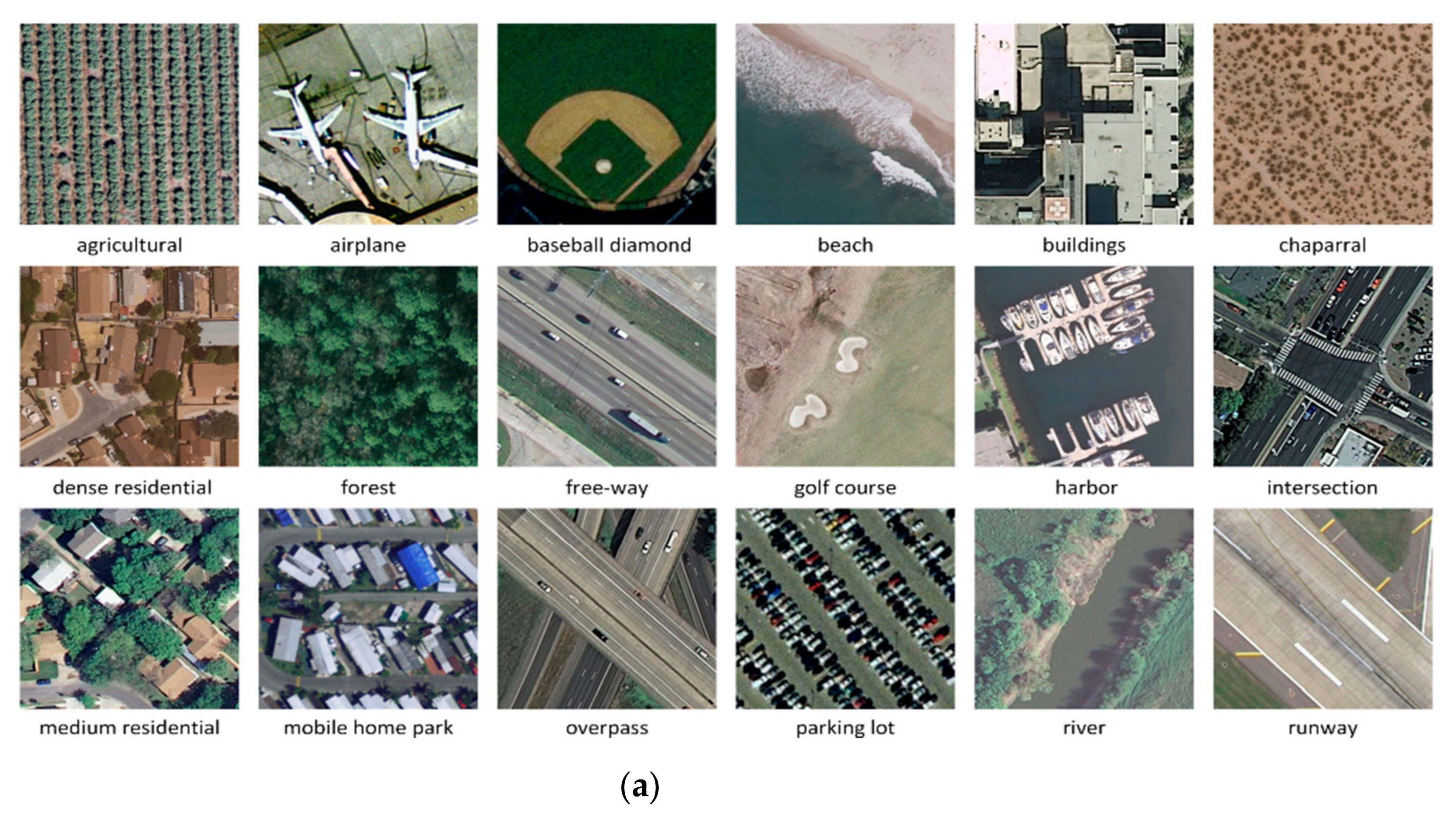
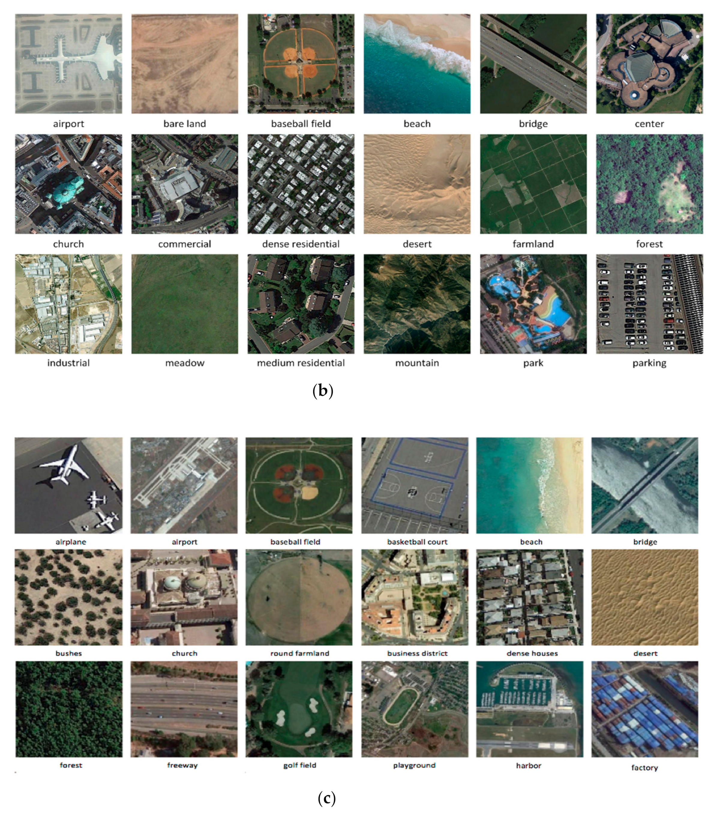
In our experiments, three well-known remote-sensing datasets are used for evaluation: Merced land-use dataset [57], Aerial image dataset (AID) [58], and the Optimal-31 [41] dataset. The characteristic of these three datasets are listed in Table 2, and samples from each dataset are shown in Figure 4.
Merced dataset: This dataset was released in 2010, and contains 2100 RGB images of 21 land-use scene classes. Each class consists of 100 images of size 256 × 256 pixels with 0.3 m resolution. The images were extracted from the United States Geological Survey National Map.
Aerial image dataset (AID) dataset: The AID dataset is a large-scale dataset of 10,000 for aerial scene images published in 2017 by Wuhan University. The dataset contains 30 different classes of 220 to 420 images per class. The images were cropped from Google Earth imagery measuring 600 × 600 pixels with a resolution varying from 8 m to about 0.5 m.
Optimal-31 dataset: This dataset was captured from Google Earth imagery covering 31 scene classes. Each class contains 60 images of size of 256 × 256 pixels in the RGB color space. The pixel resolution for the images is 0.3 m.

3.2. Experimental Setup

We conducted three sets of experiments. In the first set, we used different data augmentation strategies to assess how well the vision Transformer performs with augmented data. It is worth recalling that we used the standard cross-entropy loss for learning the weights of the network. In the second experiment, we varied the number of encoder layers and studied the relation between the network depth and model performance. Then, we investigated the impact of changing the image size on the overall accuracy of the model. Finally, we compared our results against several state-of-the-art methods.
In all experiments, we adopted the ViT-Base model following settings from [45]. The model consists of 12 encoder layers each with 12 attention heads. It has an embedding dimension of 768 and feed-forward subnetwork with size of 3072. We used a model pretrained on Imagenet-21k and then fine-tuned on Imagenet-1k. To fine-tune it on remote sensing scene data, we trained it for 30 iterations and used a minibatch size of 100. We optimized it with Adam method and set the learning rate to 0.0003. We initially fixed the image size to 224 × 224 and the patch size to 16 × 16 and got a sequence with 196 tokens length.
For comparison purposes, we evaluated the performance of the method in terms of the standard overall accuracy(OA), which represents the number of correctly classified images over the total number of images.
We conducted all the experiments on an HP Omen Station with the following specification: Central processing Unit (CPU) Intel core (TM) i9-7920× CPU @ 2.9 GHz with a RAM of 32 GB and an NVIDIA GeForce GTX 1080 Ti Graphical Processing Unit (GPU) (with 11 GB GDDR5X memory). All codes were implemented using Pytorch, which is an open-source deep neural network library written in python.

3.3. Experiment 1: Preliminary Analysis

For preliminary analysis of the Vision Transformer, we followed a low training regime and performed the experiment with minimum data. Specifically, for the AID dataset, we selected about 33 samples from each class for training, which comprised 10% of the dataset. For both Merced and Optimal31 datasets, we extracted 30 samples from each class, which comprised 30% and 50% of the first and second dataset, respectively.
We trained the network on the original and augmented images for 30 iterations. Table 3 shows the classification accuracies obtained when different data-augmentation techniques are applied. The standard data augmentation uses rotation, vertical and horizontal flipping, and random adjusting of the brightness and the color of the image. For the Cutout technique, we set the number of holes to eight and the cutout region size to 10 × 10 pixels. For the CutMix, the mixing ratio was sampled from the uniform distribution [0,1]. Finally, the hybrid data augmentation randomly selected one of the three augmentation techniques (standard, CutMix and Cutout) for each batch during the training phase.
The results in Table 3 clearly show the effectiveness of using data augmentation as widely known in the literature. In general, all strategies provided close results, but for the Merced and Optimal31 datasets, using a hybrid data augmentation yielded slightly better results with accuracy of 96.73% and 92.97%, respectively. Standard augmentation performed slightly better than other techniques for the AID dataset with 92.06%. Normally, and as the results of all the three datasets suggest, using a combination of data augmentation strategies provides slightly the best behavior.
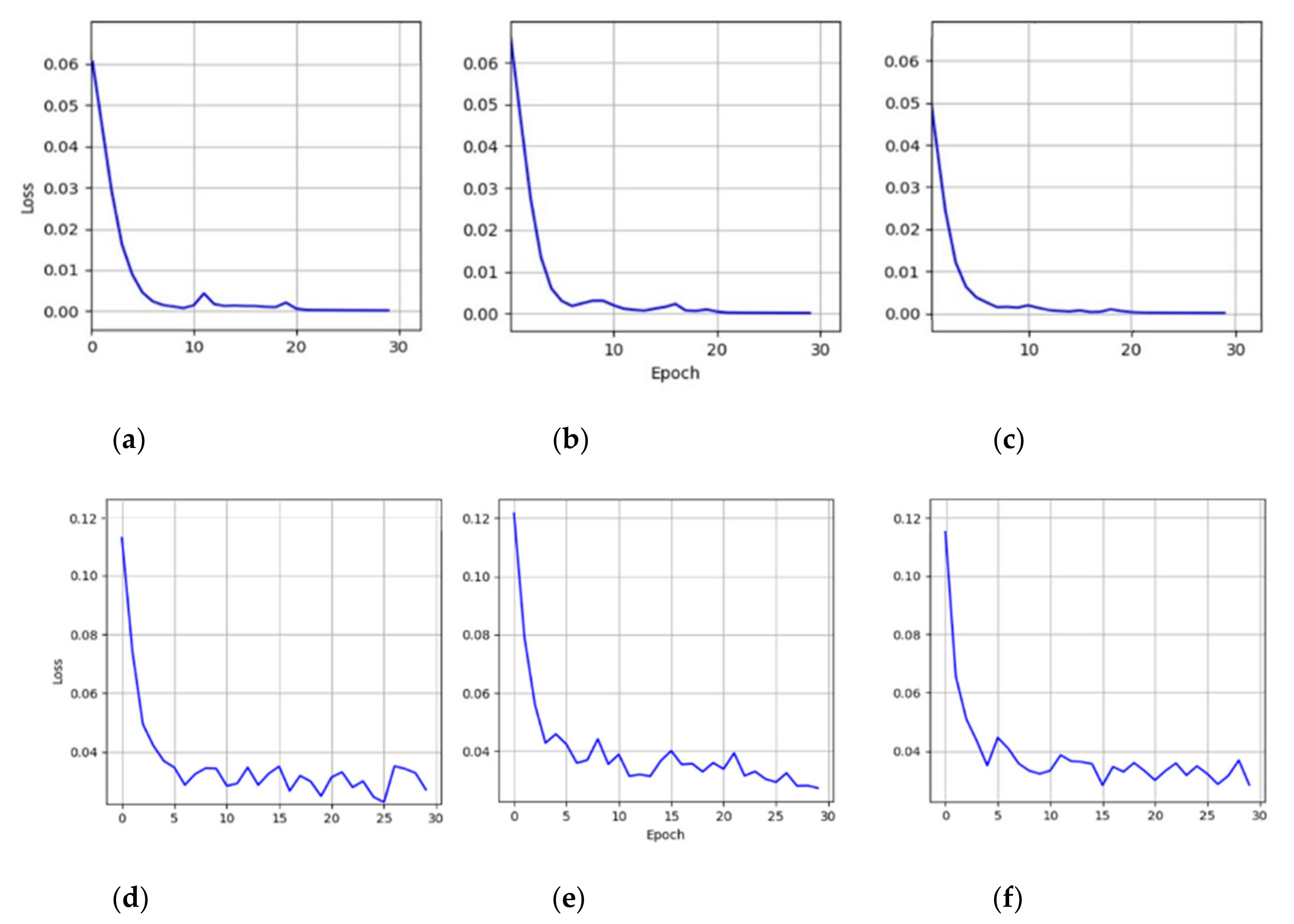
Figure 5 shows the evolution of the loss function during training with and without data augmentation. It can be seen that training the model on the original images made the loss converge smoother and faster. In contrast, when the model is trained on the augmented images the loss oscillates after the warm-up iterations and takes longer to converge.

3.4. Experiment 2: Network Compression

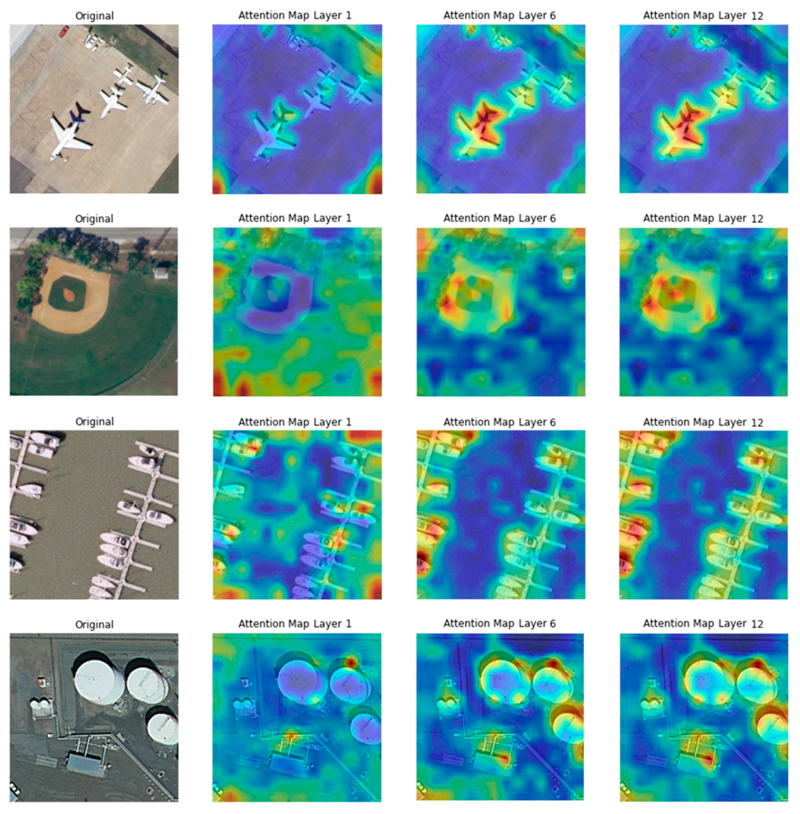
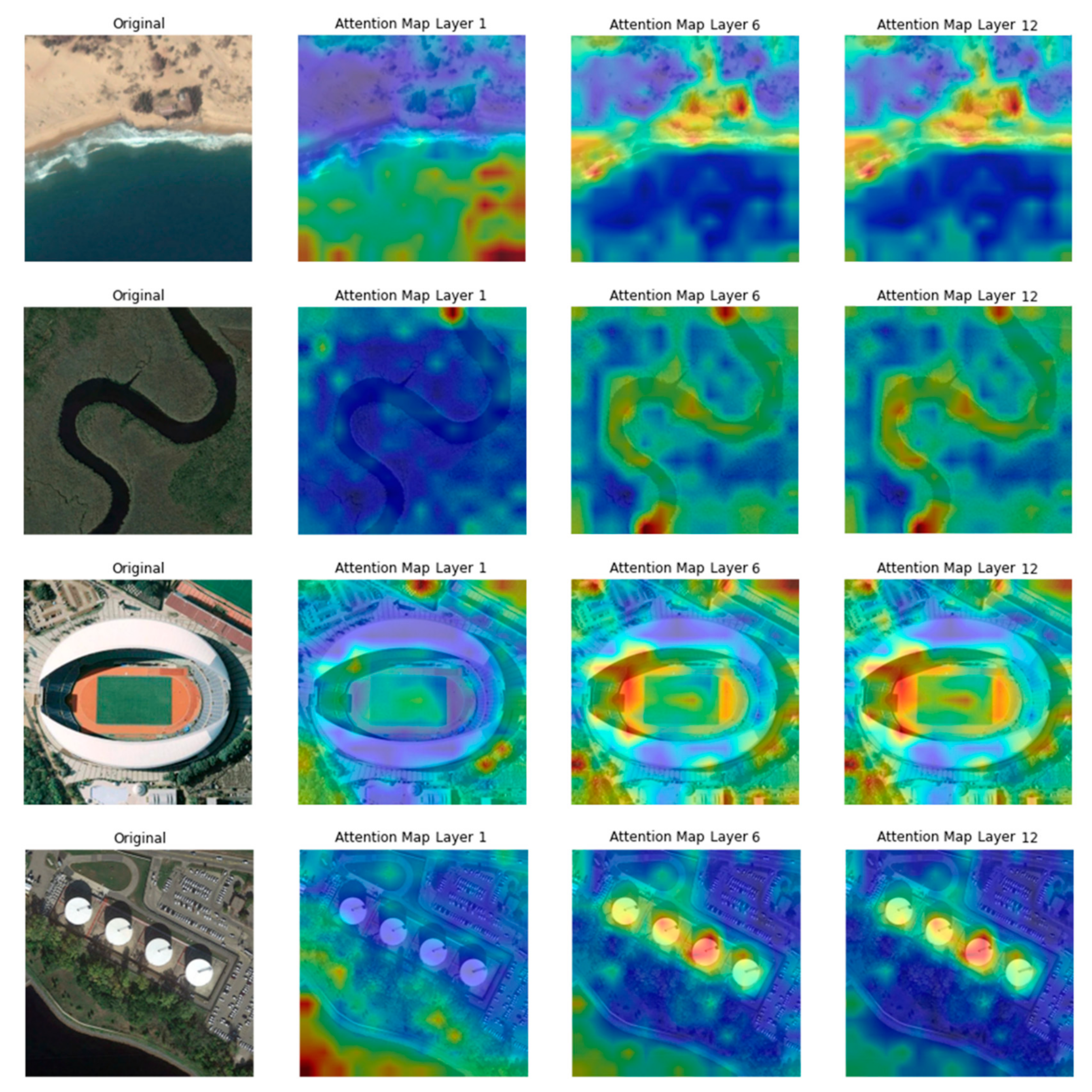
In the second set of experiments, we further analyzed the role of each layer in the encoder. First, we trained the model with the maximum number of layers (i.e., 12 layers). Then, we repeated the experiments with the same parameters, except that we took the output of each intermediate layer and projected it directly into the classifier while discarding the upper layers. In order to better understand the behavior of the network and the region attended by the attention heads in each layer, we extracted the output representations and visualized the per-layer attention maps for the Merced and AID datasets in Figure 6 and Figure 7, respectively.
Figure 6 shows four samples from the Merced dataset along with the outputs of the first, sixth, and twelfth layers. We can see that the network gradually learns to concentrate on regions that have the most representative information of the class. For instance, in the airport sample the network shows some attention on airplanes at layer 1. This progressively improved in the subsequent layers. For example, for the baseball class, the network at the first layer focused mostly on unrelated information and then the model attempted to capture the discriminative areas that is corresponding to the baseball class. For the harbor class, as the depth of the encoder increased the model tended to put more focus on the region of the boats. This change in concentration could be strongly noticed from layer 1 to layer 6. However, after layer 6 we can see that the attention to unrelated areas was reduced. This will be further confirmed in the next section.
Figure 7 shows four images from the AID dataset along with the output of three different encoder layers (layer 1, 6 and that last one). As can be seen, for the beach class the network at layer 1 mostly focuses on the sea regions. Then, the next encoder layers learn to gradually shift the attention to the beach line while gradually ignoring the unrelated regions. In addition, we observed that the attention maps provided by layer 6 are visually similarly to the one provided at the last layer. We observed also a similar behavior for the river class where the network concentrates on the river region at layer 6 and the attention slightly improves in the last layer. For the stadium image, as the encoder gets deeper it learns to localize the discriminative parts that are corresponding to the stadium class. Finally, for the tank class, we observed that the network concentrates on unrelated objects in the first layer but was able to concentrate on the tank objects at layer 6. This means that the attention improves as the encoder goes deeper.
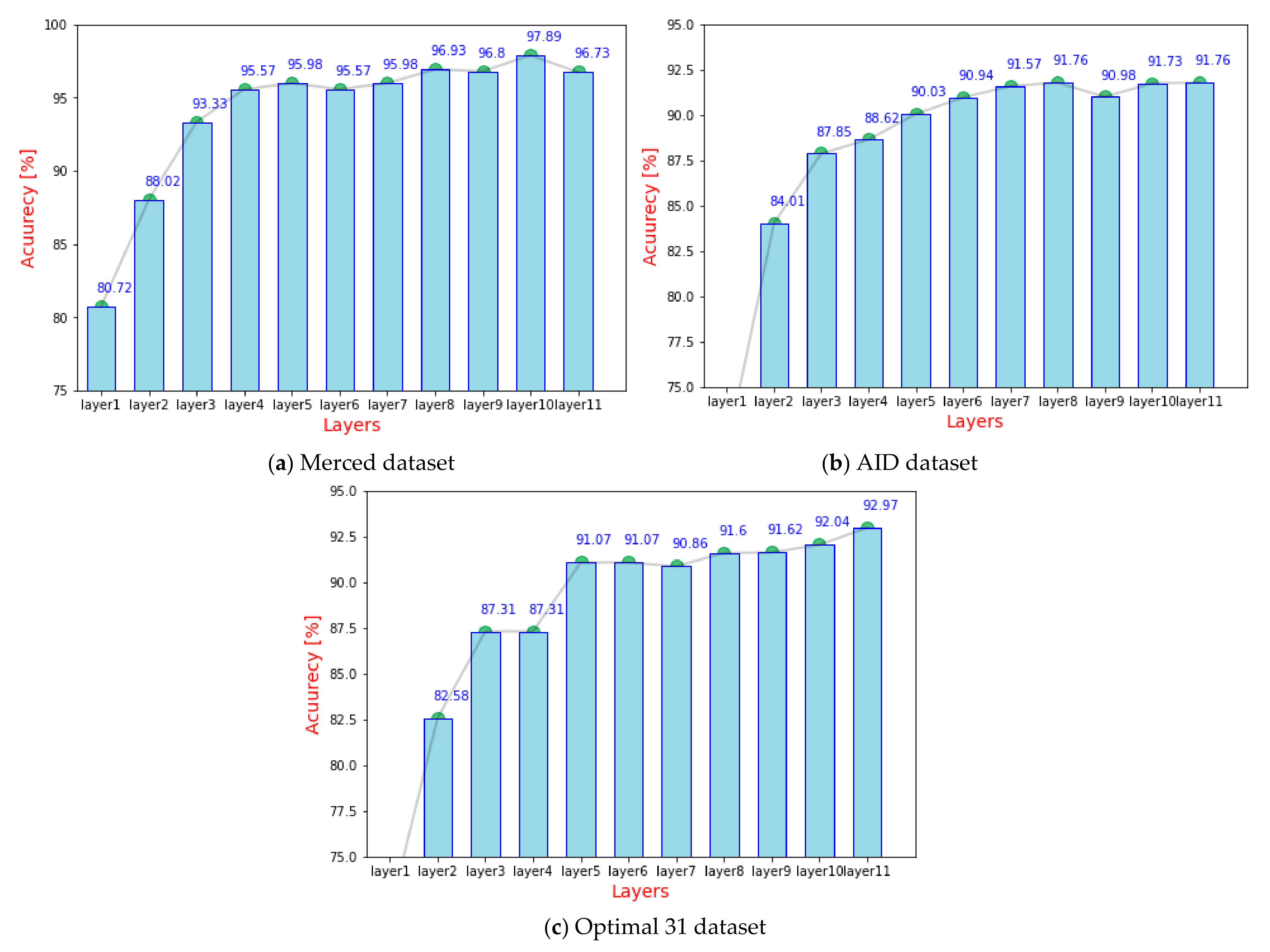
From a quantitative point of view, Figure 8 shows the classification accuracies obtained at each layer of the encoder for the Merced, AID, and Optimal 31 datasets. In general, we can see that deep encoders tend to perform better, and the classification performance is consistently increasing with the number of layers. The figure shows that using encoders with at least 5 layers is sufficient to reach 90% classification accuracy in all datasets. The subsequent layers from 6 to 12 improve the accuracy by 2%. This indicates that the earlier layers in the Vision Transformer model play the key role in extracting the discriminative representation that is required for classification.
The average results of the three datasets show that pruning the model up to layer 10 gives the best performance, with average accuracy of 93.88% compared to 93.82% with the full model. Therefore, for scene classification the last layer of the vision Transformer model can be removed without affecting the performance of the model.
More specifically, for the Optimal31 dataset the best classification accuracy can be obtained from the last layer with accuracy of 92.97%. However, it is interesting to observe that the highest accuracy can be obtained from earlier layers for the other two datasets. For example, an encoder with 10 layers gives the best classification accuracy for the Merced dataset with accuracy of 97.89%. For the AID dataset, layer 8 and 12 equally give the best results with 91.76%. These results are consistent with the qualitative results obtained from the attention maps. In next section, we will show that using only 50% of the layers can yield competing classification accuracies.

4. Discussion

We further investigate the effect of varying the image size on the performance of the model. To this end, we repeat the experiments using images with two different sizes, 224 × 224 and 384 × 384. Indeed, the vision Transformer models were pretrained on the ImageNet dataset with image size 384 × 384.
The overall accuracies and running times of the experiments are summarized in Table 4. The results clearly show an increase in image size when the model is trained with large image size. However, increasing the size can remarkably raise the training time. On average, using larger images has improved the result by 0.93% but doubled the training time from 32 to 67 min. For the Optimal31 dataset, this cost has a slight improvement on the accuracy with only 0.03%.
Finally, we compare the results of our method with the state-of-the-art results reported so far in the literature. These methods are the attention recurrent convolutional network (ARCNet) [41], in which multiple attentional features are generated using a CNN -LSTM architecture. GoogleNet extracted features classified with an SVM classifier [58]. Gated bidirectional network that uses hierarchical feature aggregation (GBNet) [31]. Multilayer stacked covariance pooling (MSCP) [59], in which features from different layers of the pretrained CNN are combined using covariance pooling and classified using an SVM. In addition, we add the results of fine-tuned VGG16 and GoogleNet models [60] and models fine-tuned with an auxiliary classifier [30].
Table 5 shows detailed comparisons for the Merced, AID, and Optimal-31 datasets, respectively. Besides these three datasets, we compare our results on the well-known NWPU dataset, which is composed of 45 classes containing 31,500 remote sensing images. Depending on the data splits reported in the literature, we set the training–testing split differently for each dataset. We termed the proposed method as V16_21k (224 × 224), and V16_21k (384 × 384) for Vision Transformer that splits images into 16 × 16, pretrained on Imagenet-21k dataset and fine-tuned with images of size 224 × 224 and 384 × 384, respectively. The results in Table 5 show that the network yields interesting results for all datasets. In particular, the configuration with large image size and smaller patch size achieves superior performance. In terms of computation time, the network takes for Merced: 153 min; AID: 347 min; Optimal31: 220 min; and NWPU: 465 min. Furthermore, Table 5 shows that the network yields very competitive results after pruning 50% of its layers.

5. Conclusions

In this work, we have proposed a method for classifying remote-sensing images based on Vision Transformers. Different from CNNs, the model is able to capture long-range dependencies among patches via an attention module. The proposed method was evaluated on four public remote-sensing image datasets, and the experimental results demonstrated the effectiveness of these new type of networks in improving the classification accuracies compared to state-of-the-art methods. Moreover, we showed that using a combination of data augmentation techniques can help in further boosting the classification accuracy. To reduce the size of the model, we presented a simple model-compression solution that prunes the network layers. For future developments, we suggest investigating alternative approaches for compressing the transformer and generating light-weight models.

Author Contributions

Y.B. designed and implemented the method, and wrote the paper. L.B., M.M.A.R., R.A.D., and N.A.A. contributed to the analysis of the experimental results and paper writing. All authors have read and agreed to the published version of the manuscript.

Funding

The authors extend their appreciation to the Researchers Supporting Project number (RSP-2020/69), King Saud University, Riyadh, Saudi Arabia.

Acknowledgments

The authors extend their appreciation to the Researchers Supporting Project number (RSP-2020/69), King Saud University, Riyadh, Saudi Arabia.

Conflicts of Interest

The authors declare no conflict of interest.

References

  1. Hu, Q.; Wu, W.; Xia, T.; Yu, Q.; Yang, P.; Li, Z.; Song, Q. Exploring the use of google earth imagery and object-based methods in land use/cover mapping. Remote Sens. 2013, 5, 6026–6042. [Google Scholar] [CrossRef] [Green Version]
  2. Toth, C.; Jóźków, G. Remote sensing platforms and sensors: A survey. ISPRS J. Photogramm. Remote Sens. 2016, 115, 22–36. [Google Scholar] [CrossRef]
  3. Hoogendoorn, S.P.; Van Zuylen, H.J.; Schreuder, M.; Gorte, B.; Vosselman, G. Microscopic traffic data collection by remote sensing. Transp. Res. Rec. 2003, 1855, 121–128. [Google Scholar] [CrossRef]
  4. Valavanis, K.P. Advances in Unmanned Aerial Vehicles: State of the Art and the Road to Autonomy; Springer Science & Business Media: Berlin, Germany, 2008; ISBN 978-1-4020-6114-1. [Google Scholar]
  5. Sheppard, C.; Rahnemoonfar, M. Real-time scene understanding for UAV imagery based on deep convolutional neural networks. In Proceedings of the 2017 IEEE International Geoscience and Remote Sensing Symposium (IGARSS), Fort Worth, TX, USA, 23–28 July 2017; pp. 2243–2246. [Google Scholar]
  6. Al-Najjar, H.A.H.; Kalantar, B.; Pradhan, B.; Saeidi, V.; Halin, A.A.; Ueda, N.; Mansor, S. Land cover classification from fused DSM and UAV images using convolutional neural networks. Remote Sens. 2019, 11, 1461. [Google Scholar] [CrossRef] [Green Version]
  7. Liu, T.; Abd-Elrahman, A.; Zare, A.; Dewitt, B.A.; Flory, L.; Smith, S.E. A fully learnable context-driven object-based model for mapping land cover using multi-view data from unmanned aircraft systems. Remote Sens. Environ. 2018, 216, 328–344. [Google Scholar] [CrossRef]
  8. Bazi, Y. Two-branch neural network for learning multi-label classification in UAV imagery. In Proceedings of the IGARSS 2019—2019 IEEE International Geoscience and Remote Sensing Symposium, Yokohama, Japan, 28 July–2 August 2019; pp. 2443–2446. [Google Scholar]
  9. Skidmore, A.K.; Bijker, W.; Schmidt, K.; Kumar, L. Use of remote sensing and GIS for sustainable land management. ITC J. 1997, 3, 302–315. [Google Scholar]
  10. Xiao, Y.; Zhan, Q. A review of remote sensing applications in urban planning and management in China. In Proceedings of the 2009 Joint Urban Remote Sensing Event, Shanghai, China, 20–22 May 2009; pp. 1–5. [Google Scholar]
  11. Daldegan, G.A.; Roberts, D.A.; de Ribeiro, F.F. Spectral mixture analysis in google earth engine to model and delineate fire scars over a large extent and a long time-series in a rainforest-savanna transition zone. Remote Sens. Environ. 2019, 232, 111340. [Google Scholar] [CrossRef]
  12. Ahonen, T.; Hadid, A.; Pietikainen, M. Face description with local binary patterns: Application to face recognition. IEEE Trans. Pattern Anal. Mach. Intell. 2006, 28, 2037–2041. [Google Scholar] [CrossRef]
  13. Dalal, N.; Triggs, B. Histograms of oriented gradients for human detection. In Proceedings of the 2005 IEEE Computer Society Conference on Computer Vision and Pattern Recognition (CVPR’05), San Diego, CA, USA, 20–25 June 2005; IEEE: San Diego, CA, USA, 2005; Volume 1, pp. 886–893. [Google Scholar]
  14. Li, Q.; Qi, S.; Shen, Y.; Ni, D.; Zhang, H.; Wang, T. Multispectral image alignment with nonlinear scale-invariant keypoint and enhanced local feature matrix. IEEE Geosci. Remote Sens. Lett. 2015, 12, 1551–1555. [Google Scholar] [CrossRef]
  15. Sivic, J.; Russell, B.C.; Efros, A.A.; Zisserman, A.; Freeman, W.T. Discovering objects and their location in images. In Proceedings of the Tenth IEEE International Conference on Computer Vision (ICCV’05), Beijing, China, 17–21 October 2005; Volume 1, pp. 370–377. [Google Scholar]
  16. Huang, L.; Chen, C.; Li, W.; Du, Q. Remote sensing image scene classification using multi-scale completed local binary patterns and fisher vectors. Remote Sens. 2016, 8, 483. [Google Scholar] [CrossRef] [Green Version]
  17. Imbriaco, R.; Sebastian, C.; Bondarev, E.; de With, P.H.N. Aggregated deep local features for remote sensing image retrieval. Remote Sens. 2019, 11, 493. [Google Scholar] [CrossRef] [Green Version]
  18. Diao, W.; Sun, X.; Zheng, X.; Dou, F.; Wang, H.; Fu, K. Efficient saliency-based object detection in remote sensing images using deep belief networks. IEEE Geosci. Remote Sens. Lett. 2016, 13, 137–141. [Google Scholar] [CrossRef]
  19. Chen, Y.; Lin, Z.; Zhao, X.; Wang, G.; Gu, Y. Deep learning-based classification of hyperspectral data. IEEE J. Sel. Top. Appl. Earth Obs. Remote Sens. 2014, 7, 2094–2107. [Google Scholar] [CrossRef]
  20. Nogueira, K.; Miranda, W.O.; Santos, J.A.D. Improving spatial feature representation from aerial scenes by using convolutional networks. In Proceedings of the 2015 28th SIBGRAPI Conference on Graphics, Patterns and Images, Salvador, Brazil, 26–29 August 2015; pp. 289–296. [Google Scholar]
  21. Marmanis, D.; Datcu, M.; Esch, T.; Stilla, U. Deep learning earth observation classification using imagenet pretrained networks. IEEE Geosci. Remote Sens. Lett. 2016, 13, 105–109. [Google Scholar] [CrossRef] [Green Version]
  22. Maggiori, E.; Tarabalka, Y.; Charpiat, G.; Alliez, P. Convolutional neural networks for large-scale remote-sensing image classification. IEEE Trans. Geosci. Remote Sens. 2017, 55, 645–657. [Google Scholar] [CrossRef] [Green Version]
  23. Lakhal, M.I.; Çevikalp, H.; Escalera, S.; Ofli, F. Recurrent neural networks for remote sensing image classification. IET Comput. Vis. 2018, 12, 1040–1045. [Google Scholar] [CrossRef] [Green Version]
  24. Zhu, L.; Chen, Y.; Ghamisi, P.; Benediktsson, J.A. Generative adversarial networks for hyperspectral image classification. IEEE Trans. Geosci. Remote Sens. 2018, 56, 5046–5063. [Google Scholar] [CrossRef]
  25. Feng, J.; Yu, H.; Wang, L.; Cao, X.; Zhang, X.; Jiao, L. Classification of hyperspectral images based on multiclass spatial–spectral generative adversarial networks. IEEE Trans. Geosci. Remote Sens. 2019, 57, 5329–5343. [Google Scholar] [CrossRef]
  26. Mou, L.; Lu, X.; Li, X.; Zhu, X.X. Nonlocal graph convolutional networks for hyperspectral image classification. IEEE Trans. Geosci. Remote Sens. 2020, 1–12. [Google Scholar] [CrossRef]
  27. Hu, W.; Li, H.; Pan, L.; Li, W.; Tao, R.; Du, Q. Spatial–spectral feature extraction via deep ConvLSTM neural networks for hyperspectral image classification. IEEE Trans. Geosci. Remote Sens. 2020, 58, 4237–4250. [Google Scholar] [CrossRef]
  28. Bi, Q.; Qin, K.; Li, Z.; Zhang, H.; Xu, K.; Xia, G.-S. A multiple-instance densely-connected ConvNet for aerial scene classification. IEEE Trans. Image Process. 2020, 29, 4911–4926. [Google Scholar] [CrossRef]
  29. Yu, Y.; Li, X.; Liu, F. Attention GANs: Unsupervised deep feature learning for aerial scene classification. IEEE Trans. Geosci. Remote Sens. 2020, 58, 519–531. [Google Scholar] [CrossRef]
  30. Bazi, Y.; Al Rahhal, M.M.; Alhichri, H.; Alajlan, N. Simple yet effective fine-tuning of deep CNNs using an auxiliary classification loss for remote sensing scene classification. Remote Sens. 2019, 11, 2908. [Google Scholar] [CrossRef] [Green Version]
  31. Sun, H.; Li, S.; Zheng, X.; Lu, X. Remote sensing scene classification by gated bidirectional network. IEEE Trans. Geosci. Remote Sens. 2019, 1–15. [Google Scholar] [CrossRef]
  32. Liu, Y.; Liu, Y.; Ding, L. Scene classification based on two-stage deep feature fusion. IEEE Geosci. Remote Sens. Lett. 2018, 15, 183–186. [Google Scholar] [CrossRef]
  33. Yu, Y.; Liu, F. A Two-Stream Deep Fusion Framework for High-Resolution Aerial Scene Classification. Available online: https://www.hindawi.com/journals/cin/2018/8639367/ (accessed on 20 November 2020).
  34. Cheng, G.; Yang, C.; Yao, X.; Guo, L.; Han, J. When deep learning meets metric learning: Remote sensing image scene classification via learning discriminative CNNs. IEEE Trans. Geosci. Remote Sens. 2018, 56, 2811–2821. [Google Scholar] [CrossRef]
  35. Xue, W.; Dai, X.; Liu, L. Remote sensing scene classification based on multi-structure deep features fusion. IEEE Access 2020, 8, 28746–28755. [Google Scholar] [CrossRef]
  36. Wang, Q.; Li, B.; Xiao, T.; Zhu, J.; Li, C.; Wong, D.F.; Chao, L.S. Learning deep transformer models for machine translation. In Proceedings of the 57th Annual Meeting of the Association for Computational Linguistics, Fortezza da Florence, Italy, 28 July–2 August 2019; pp. 1810–1822. [Google Scholar]
  37. Dai, Z.; Yang, Z.; Yang, Y.; Carbonell, J.; Le, Q.; Salakhutdinov, R. Transformer-XL: Attentive language models beyond a fixed-length context. In Proceedings of the 57th Annual Meeting of the Association for Computational Linguistics, Fortezza da Florence, Italy, 28 July–2 August 2019; pp. 2978–2988. [Google Scholar]
  38. Chen, N.; Watanabe, S.; Villalba, J.A.; Zelasko, P.; Dehak, N. Non-autoregressive transformer for speech recognition. IEEE Signal Process. Lett. 2020, 28, 121–125. [Google Scholar] [CrossRef]
  39. Vaswani, A.; Shazeer, N.; Parmar, N.; Uszkoreit, J.; Jones, L.; Gomez, A.N.; Kaiser, Ł.; Polosukhin, I. Attention is all you need. Adv. Neural Inf. Process. Syst. 2017, 30, 5998–6008. [Google Scholar]
  40. Bello, I.; Zoph, B.; Vaswani, A.; Shlens, J.; Le, Q.V. Attention Augmented Convolutional Networks. In Proceedings of the 2019 IEEE/CVF International Conference on Computer Vision (ICCV), Seoul, Korea, 27 October–2 November 2019; pp. 3285–3294. [Google Scholar]
  41. Wang, Q.; Liu, S.; Chanussot, J.; Li, X. Scene classification with recurrent attention of VHR remote sensing images. IEEE Trans. Geosci. Remote Sens. 2019, 57, 1155–1167. [Google Scholar] [CrossRef]
  42. Wu, B.; Xu, C.; Dai, X.; Wan, A.; Zhang, P.; Tomizuka, M.; Keutzer, K.; Vajda, P. Visual transformers: Token-based image representation and processing for computer vision. arXiv 2020, arXiv:2006.03677. [Google Scholar]
  43. Ramachandran, P.; Parmar, N.; Vaswani, A.; Bello, I.; Levskaya, A.; Shlens, J. Stand-alone self-attention in vision models. arXiv 2019, arXiv:1906.05909. [Google Scholar]
  44. Chen, M.; Radford, A.; Child, R.; Wu, J.; Jun, H.; Luan, D.; Sutskever, I. Generative pretraining from pixels. In Proceedings of the 37th International Conference on Machine Learning, Vienna, Austrlia, 12–18 July 2020; pp. 1691–1703. [Google Scholar]
  45. Dosovitskiy, A.; Beyer, L.; Kolesnikov, A.; Weissenborn, D.; Zhai, X.; Unterthiner, T.; Dehghani, M.; Minderer, M.; Heigold, G.; Gelly, S.; et al. An image is worth 16 × 16 words: Transformers for image recognition at scale. arXiv 2020, arXiv:2010.11929. [Google Scholar]
  46. He, J.; Zhao, L.; Yang, H.; Zhang, M.; Li, W. HSI-BERT: Hyperspectral image classification using the bidirectional encoder representation from transformers. IEEE Trans. Geosci. Remote Sens. 2020, 58, 165–178. [Google Scholar] [CrossRef]
  47. Devlin, J.; Chang, M.-W.; Lee, K.; Toutanova, K. BERT: Pre-training of deep bidirectional transformers for language understanding. In Proceedings of the 2019 Conference of the North American Chapter of the Association for Computational Linguistics: Human Language Technologies, Minneapolis, MI, USA, 2–7 June 2019; Long and Short Papers. Volume 1, pp. 4171–4186. [Google Scholar]
  48. Cubuk, E.D.; Zoph, B.; Mane, D.; Vasudevan, V.; Le, Q.V. AutoAugment: Learning augmentation strategies from data. In Proceedings of the 2019 IEEE/CVF Conference on Computer Vision and Pattern Recognition (CVPR), Long Beach, CA, USA, 15–21 June 2019; IEEE: Long Beach, CA, USA, 2019; pp. 113–123. [Google Scholar]
  49. Jackson, P.T.; Atapour-Abarghouei, A.; Bonner, S.; Breckon, T.P.; Obara, B. Style Augmentation: Data Augmentation via Style Randomization. In Proceedings of the 2019 IEEE Conference on Computer Vision and Pattern Recognition (CVPR), Long Beach, CA, USA, 16–20 June 2019. [Google Scholar]
  50. Bowles, C.; Chen, L.; Guerrero, R.; Bentley, P.; Gunn, R.; Hammers, A.; Dickie, D.A.; Hernández, M.V.; Wardlaw, J.; Rueckert, D. GAN augmentation: Augmenting training data using generative adversarial networks. arXiv 2018, arXiv:1810.10863. [Google Scholar]
  51. DeVries, T.; Taylor, G.W. Improved regularization of convolutional neural networks with cutout. arXiv 2017, arXiv:1708.04552. [Google Scholar]
  52. Zhang, H.; Cisse, M.; Dauphin, Y.N.; Lopez-Paz, D. Mixup: Beyond empirical risk minimization. arXiv 2018, arXiv:1710.09412. [Google Scholar]
  53. Yun, S.; Han, D.; Chun, S.; Oh, S.J.; Yoo, Y.; Choe, J. CutMix: Regularization strategy to train strong classifiers with localizable features. In Proceedings of the 2019 IEEE/CVF International Conference on Computer Vision (ICCV), Seoul, Korea, 27 October–2 November 2019; pp. 6022–6031. [Google Scholar]
  54. Hinton, G.; Vinyals, O.; Dean, J. Distilling the knowledge in a neural network. arXiv 2015, arXiv:1503.02531. [Google Scholar]
  55. Han, S.; Mao, H.; Dally, W.J. Deep compression: Compressing deep neural networks with pruning, trained quantization and huffman coding. arXiv 2016, arXiv:1510.00149. [Google Scholar]
  56. Wu, J.; Leng, C.; Wang, Y.; Hu, Q.; Cheng, J. Quantized Convolutional Neural Networks for Mobile Devices. In Proceedings of the 2016 IEEE Conference on Computer Vision and Pattern Recognition (CVPR), Las Vegas, NV, USA, 27–30 June 2016; pp. 4820–4828. [Google Scholar]
  57. Yang, Y.; Newsam, S. Bag-of-visual-words and spatial extensions for land-use classification. In Proceedings of the 18th SIGSPATIAL International Conference on Advances in Geographic Information Systems—GIS ’10, San Jose, CA, USA, 2–5 November 2010; p. 270. [Google Scholar]
  58. Xia, G.; Hu, J.; Hu, F.; Shi, B.; Bai, X.; Zhong, Y.; Zhang, L.; Lu, X. AID: A benchmark data set for performance evaluation of aerial scene classification. IEEE Trans. Geosci. Remote Sens. 2017, 55, 3965–3981. [Google Scholar] [CrossRef] [Green Version]
  59. He, N.; Fang, L.; Li, S.; Plaza, A.; Plaza, J. Remote sensing scene classification using multilayer stacked covariance pooling. IEEE Trans. Geosci. Remote Sens. 2018, 56, 6899–6910. [Google Scholar] [CrossRef]
  60. Cheng, G.; Han, J.; Lu, X. Remote sensing image scene classification: Benchmark and state of the art. Proc. IEEE 2017, 105, 1865–1883. [Google Scholar] [CrossRef] [Green Version]
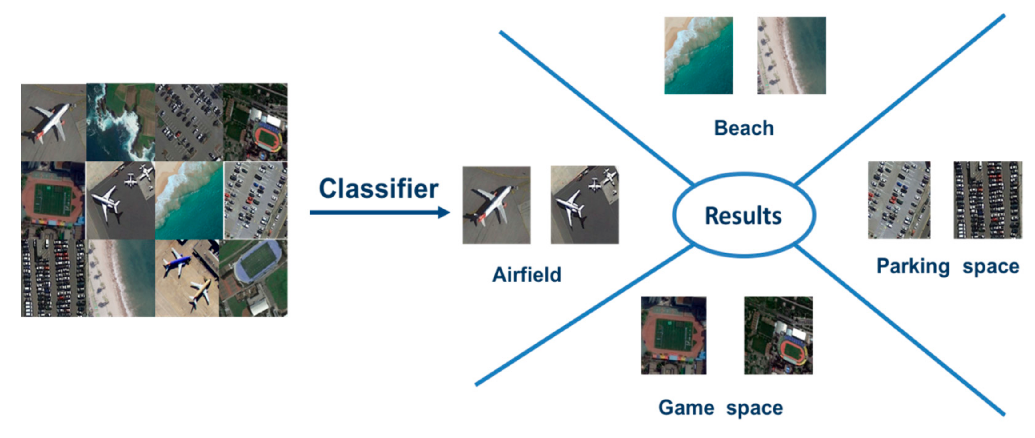
Figure 1. Remote sensing scene classification.
Remotesensing 13 00516 g001
Figure 2. The Vision Transformer architecture: (a) the main architecture of the model; (b) the Transformer encoder module; (c) the Multiscale-self attention (MSA) head, and (d) the self-attention (SA) head.
Remotesensing 13 00516 g002
Figure 3. Examples of applying data augmentation techniques on Merced dataset.
Remotesensing 13 00516 g003
Figure 4. Some example images from (a) Merced dataset. (b) AID dataset. (c) Optimal-31.
Remotesensing 13 00516 g004aRemotesensing 13 00516 g004b
Figure 5. Loss function without data augmentation for: (a) Merced, (b) AID, and (c) Optimal31, and with data augmentation for: (d) Merced, (e) AID, and (f) Optimal31.
Remotesensing 13 00516 g005
Figure 6. The class attention maps resulted from different encoder’s layers for the Merced dataset.
Remotesensing 13 00516 g006
Figure 7. The class attention maps resulted from different encoder’s layers for the AID dataset.
Remotesensing 13 00516 g007
Figure 8. Relative change in model classification accuracy with respect to the encoder layers for the (a) Merced, (b) AID, and (c) Optimal-31 datasets.
Remotesensing 13 00516 g008
Table 1. Parameter statistics for the Base, Large and Huge variants of Vision Transformer.
ModelNumber of LayersHidden Size DMLP SizeHeadsNumber of Parameters
ViT-Base1276830721286 M
ViT-Large241024409616307 M
ViT-Huge321280512016632 M
Table 2. Characteristic of the datasets.
DatasetNumber of ClassesNumber of Images per ClassImage SizeYear
Merced21100256 × 2562010
AID30220~420600 × 6002017
Optimal 313160256 × 2562019
Table 3. Classification results on: (A): Merced dataset (30% train set), AID (10% trainset) and Optimal 31 (50% Train set). Image size: 224 × 224.
With Augmentation
DatasetClean ImagesStandardCutMixCutoutHybrid
Merced94.5596.3296.6695.4496.73
AID89.3192.0690.5091.6291.76
Optimal3188.2791.4392.4492.2592.97
Average90.7193.2793.2093.3093.82
Table 4. Overall accuracies and training times obtained using different image size on different remote datasets.
Dataset224 × 224384 × 384
Merced96.73
30 min
97.43
46 min
AID91.76
43 min
92.94
88 min
Optimal3192.76
25 min
92.79
68 min
Average93.45
32.66 min
94.38
67.33 min
Table 5. Comparison with state-of-the-art methods.
Datasets
MethodMerced
(50% Train)
AID
(20% Train)
Optimal31
(80% Train)
NWPU
(10% Train)
ARCNet-VGG16 [41]96.81 ± 0.1488.75 ± 0.4092.70 ± 0.35-
ARCNet- AlexNet [41]--85.75 ± 0.35-
ARCNet- ResNet [41]--91.28 ± 0.45-
GoogLeNet+SVM [58]92.70 ± 0.6083.44 ± 0.40--
GBNet + global feature [31]97.05 ± 0.1992.20 ± 0.2393.28 ± 0.27-
VGG-16+MSCP [59]98.36 ± 0.5891.52 ± 0.21--
Fine-tuning VGG16 [31] 96.57 ± 0.3889.49 ± 0.3489.52 ± 0.2687.15 ± 0.45
Fine-tuning GoogLeNet [60]--82.57 ± 0.1282.57 ± 0.12
Inception-v3-aux [30]97.63 ± 0.2093.52 ± 0.2194.13 ± 0.3589.32 ± 0.33
GoogLeNet-aux [30]97.90 ± 0.3493.25 ± 0.3393.11 ± 0.5589.22 ± 0.25
EfficientNetB0-aux [30]98.01 ± 0.4593.69± 0.1193.97 ± 0.1389.96 ± 0.27
EfficientNetB3-aux [30]98.22 ± 0.4994.19 ± 0.1594.51 ± 0.7591.08 ± 0.14
Proposed V32_21k [384 × 384]97.74 ± 0.1095.51 ± 0.5794.62 ± 0.3892.81 ± 0.17
Proposed V16_21k [224 × 224]98.14 ± 0.4794.97 ±0.0195.07 ± 0.1292.60 ± 0.10
Proposed V16_21k [384 × 384]98.49 ± 0.4395.86 ± 0.2895.56 ± 0.1893.83 ± 0.46
Proposed V16_21k [384 × 384] [pruning 50%]97.90 ± 0.1094.27 ± 1.4195.30 ± 0.5893.05 ± 0.46
Publisher’s Note: MDPI stays neutral with regard to jurisdictional claims in published maps and institutional affiliations.