Adopting “Difference-in-Differences” Method to Monitor Crop Response to Agrometeorological Hazards with Satellite Data: A Case Study of Dry-Hot Wind

Abstract

Rapid changing climate has increased the risk of natural hazards and threatened global and regional food security. Near real-time monitoring of crop response to agrometeorological hazards is fundamental to ensuring national and global food security. However, quantifying crop responses to a specific hazard in the natural environment is still quite challenging, especially over large areas, due to the lack of tools to separate the independent impact of the hazard on crops from other confounding factors. In this study, we present a general difference-in-differences (DID) framework to monitor crop response to agrometeorological hazards at near real-time using widely accessible remotely sensed vegetation indices (VIs). To demonstrate the effectiveness of the DID framework, we applied it in quantifying the dry-hot wind impact on winter wheat in northern China as a case study using the VIs calculated from the MODIS data. The monitoring results for three years with varying severity levels of dry-hot events (i.e., 2007, 2013, and 2014) demonstrated that the framework can effectively detect winter wheat growing areas affected by dry-hot wind hazards. The estimated damage shows a notable relationship (R² = 0.903, p < 0.001) with the dry-hot wind intensity calculated from meteorological data, suggesting the effectiveness of the method when field data on a large scale is not available for direct validation. The main advantage of this method is that it can effectively isolate the impact of a specific hazard (i.e., dry-hot wind in the case study) from the mixed signals caused by other confounding factors. This general DID framework is very flexible and can be easily extended to other natural hazards and crop types with proper adjustment. Not only can this framework improve the crop yield forecast but also it can provide near real-time assessment for farmers to adapt their farming practice to mitigate impacts of agricultural hazards.

1. Introduction

The rapidly changing climate has affected global and regional food security due to increased temperatures, changing precipitation patterns, and more frequent extreme events [1]. Near real-time monitoring of crop conditions is thus fundamental to ensure national and global food security, especially under the increasing risk of natural hazards caused by climate change. Earth Observation Systems (EOS) play a significant role in monitoring crop response to natural hazards, such as drought, flooding, frost, and heatwaves, at near real-time [2,3,4,5]. Previous studies have demonstrated that vegetation indices (VIs) derived from remotely sensed data show strong responses to the physiological and structural change of crops when they are under stresses [6,7,8]. Accordingly, VIs have been widely used for crop stress monitoring (see the review article in [9]).

Although VI data have shown great potential for monitoring crop growing conditions, it is challenging to quantify crop response to specific agrometeorological hazards (called as hazard below). Currently, there are two methods to evaluate crop response to specific hazards using VI data. The first method uses the change of VI after a hazard compared to the pre-hazard VI values in the same year to quantify crop response [10], while the second method uses the change of VI between the hazard year and a historical hazard-free year during the same growing period [11,12]. For the first method, how to determine the proper VI value that represents the most severe hazard damage is very challenging due to other confounding factors that may also cause VI reduction (e.g., cloud contamination, diseases, and pests). For the second method, the difference in VI between the hazard year and the hazard-free year is a combination of the crop response to the hazard damage and interannual variations of climatic conditions and phenological stages. Therefore, it is challenging to quantify the real effect of a hazard on the crop from the mixed-signal if the interannual variations of climatic conditions and phenological stages are not properly accounted for [5]. Currently, there is still a lack of a remote sensing-based framework that can effectively isolate the independent impact of a hazard on crops.

The “Difference-in-Differences” (DID) method from social sciences addresses a similar issue to assess the independent impact of a policy on the subject of study. DID is a robust nonexperimental tool in econometrics and quantitative research that can evaluate the causal effect of programs or policies [13,14,15,16]. The essence of the method is to control the double difference (changes over time and over control group) during the assessment [16]. The independent effect of a specific policy or treatment is quantified by comparing the difference in outcome after and before the intervention for the group affected by the treatment to the difference of the unaffected group (or control group) [17] (more details of DID can be found in Section 3). When we apply DID to crop condition monitoring, it can provide an effective way to isolate the VI change caused by a hazard from the VI change caused by other compounding factors, thus, allowing us to quantify crop response to a specific hazard. To the best of our knowledge, DID has not yet been adopted in agriculture remote sensing field.

This research aims to establish a general DID framework to monitor crop response to hazards at near real-time using widely accessible remotely sensed VI data. To demonstrate the effectiveness of the monitoring framework, we used winter wheat as the crop of interest in this study because this crop is the main staple food crop in China and its production plays an essential role in ensuring China’s food security [18,19]. As a case study, we applied the proposed framework to assess winter wheat response to the dry-hot wind (also called heat stress). The dry-hot wind is a type of agrometeorological hazard with high air temperature, low air humidity, and certain wind speed. According to the Chinese meteorological industry standard [20], if the maximum temperature is greater than 31 ℃, the relative air humidity is less than 30%, and the wind speed is greater than 3 m/s, winter wheat is at risk of exposure to dry-hot wind events. This type of hazard usually occurs during the reproductive and grain-filling periods of winter wheat and can cause severe impacts both on crop yield and quality for winter wheat [21,22,23,24]. We chose dry-hot wind for this case study because recent global warming has increased the frequency and intensity of dry-hot wind events, thus causing urgent need of an effective monitoring framework [25,26,27,28]. An effective monitoring framework of winter wheat response to dry-hot wind will not only improve crop yield forecast but also provide near real-time information for farmers to mitigate damage caused by dry-hot wind [7].

Despite the urgent need, quantifying the response of winter wheat to dry-hot wind is quite challenging, especially over large areas. Previous studies primarily focused on controlled field experiments and crop model simulations [29,30]. Both field experiments and crop model studies are indispensable for understanding the physiological mechanisms responsible for damages caused by dry-hot wind. However, they are not fully capable of representing crop response to dry-hot wind in a natural environment over large areas. For example, field experiments tend to be conducted over a limited set of sites which require intensive labor for data collection and analysis. It may provide the most accurate results on crop damage of a specific event at local scale, but it is very challenging to apply it over large areas due to its requirement of intensive labor. On the hand, process-based models have been used to monitor crop responses to meteorological and soil conditions based on given management practices over certain regions (e.g., Monitoring Agricultural Resources (Europe) [31,32] and Yield Prophet (Australia) [33]. Nonetheless, it is very challenging to use such models to represent crop responses to extreme events like dry-hot wind over large areas [29]. Additionally, it is still controversial whether crop models can be well generalized to large areas [34]. Remote sensing can offer relevant information over large areas in a rapid and cost-effective manner. The full suite of information provided by field data, satellite-based system, and process-based crop model can provide the most comprehensive and accurate information of crop growing status and its response to extreme events. Figure 1 shows the growth cycle of winter wheat from the remote sensing perspective using the time series of VI and possible hazards that may occur at different growth stages.

We conducted a literature search in the Web of Science Core Collection using “remote sensing” (as the topic), “winter wheat”, and various agrometeorological hazards (in the title) in all available years (i.e., 1980–2020). The number of returned articles for different hazards is also listed in Figure 1. Overall, we only found 20 articles addressing the five major hazards, with only one study focusing on the dry-hot wind. This study uses remotely sensed data to investigate the responses of crop growth duration and leaf area index (LAI) of winter wheat to heat stress during the reproductive stage [22]. However, the retrospective study does not provide the capacity for rapid monitoring of high-temperature damage to winter wheat by remote sensing. A potential reason for the scarcity of relevant research is that dry-hot wind usually occurs at the post-heading stage when VI displays a downward trend. Thus, the drop of VI value caused by dry-hot wind is usually superimposed on the intrinsic downward part of the VI curve (Figure 1), making it very difficult to isolate the impact from the dry-hot event. How to isolate the reduction of VI caused by dry-hot wind from the mixed signal of the observed VI curve is the primary issue to effectively monitor the winter wheat response to dry-hot wind using remotely sensed VI data. Fortunately, the DID method has the potential to disentangle the mixed signal for quantifying wheat response to dry-hot wind based on its principle [16,17].

2. Theoretical Basis for Remote Sensing Monitoring of Dry-Hot Wind

2.1. Spectral Response to Dry-Hot Wind

Dry-hot wind can lead to shortened grill-filling period and pollen viability reduction for winter wheat. Its main physiological impact on wheat is accelerated leaf senescence, including inactivation of photosynthetic enzymes, production of chloroplast oxidative damage, and reduced leaf water content [35]. These physiological responses can eventually be observed in the spectral reflectance of winter wheat. Spectral measurement in the field experiments revealed that the reflectance of winter wheat decreases significantly in the near-infrared (NIR) band and increases slightly in the visible bands (i.e., blue, green, and red) [36,37]. These spectral responses are more pronounced under the severe dry-hot wind treatment than under the mild dry-hot wind treatment. Therefore, the observed VI loss can reflect chlorophyll deterioration, reduced photochemical efficiency, decreased leaf water content, shortened grill-filling period (e.g., early end of grain-filling), and eventual yield loss caused by dry-hot wind to some extent.

To confirm whether the spectral response to dry-hot wind can also be observed in Moderate Resolution Imaging Spectrometer (MODIS) data, we selected wheat pixels affected by dry-hot wind events with different levels of severity to analyze their reflectance response to dry-hot wind events using seven spectral bands in the MODIS bidirectional reflectance distribution function (BRDF)-adjusted daily reflectance product (MCD43A4). The dry-hot wind severity is derived from meteorological data using Chinese national meteorological industry standard [20]. Different levels of dry-hot wind severity are calculated based on

Table 1. The Chinese national meteorological industry standard for determining different levels of dry-hot wind severity. RSM_20cm represents 20cm relative soil moisture (%), which is the percentage of soil water content to the field water holding capacity. T_max represents maximum air temperature (°C), RAH₁₄ represents relative air humidity (%) at 14:00, WS₁₄ represents wind speed (m/s) at 14:00.

Regions	RSM20 cm	Mild			Moderate			Severe
		Tmax	RAH14	WS14	Tmax	RAH14	WS14	Tmax	RAH14	WS14
Wheat Region in North China	<60	≥31	≤30	≥3	≥32	≤25	≥3	≥35	≤25	≥3
	≥60	≥33	≤30	≥3	≥35	≤25	≥3	≥36	≤30	≥3

.

As shown in Figure 2a,c,e, the reflectance of winter wheat in the NIR band (band 2 in MCD43A4 product) decreases, while reflectance in the visible bands (bands 1, 3, 4 in MDC43A4 product) increases after experiencing the dry-hot wind. The magnitude of the reflectance change is also more pronounced as the severity of the dry-hot wind increases, which is consistent with the results of the controlled field experiments [36,37]. Additionally, the reflectance of the short-wave infrared band (SWIR1,1628–1652 nm, band 6 in MCD43A4 product) increases notably, which suggests the reduced leaf water content caused by the dry-hot wind [35]. These spectral changes, especially of the red, NIR, and SWIR1 bands, are evident in the time series of MODIS data, as shown in Figure 2b,d,f, indicating the potential of using MODIS data to monitor the response of winter wheat to dry-hot wind at a large scale.

2.2. VI Response to Dry-Hot Wind

VI can be employed to further enhance the above spectral responses of winter wheat to the dry-hot wind. Historically, the normalized difference vegetation index (NDVI) and the enhanced vegetation index (EVI) have been widely used for remote sensing monitoring of vegetation growth status [38,39]. However, both NDVI and EVI do not use the short-wave infrared (SWIR) band, which responds strongly to the dry-hot wind because of its sensitivity to plant leaf water content. Conversely, the normalized difference phenology index (NDPI) uses the SWIR1 band in its calculation, which was originally developed to improve phenology monitoring for the deciduous ecosystem by minimizing the impact of snow and soil background on VI [40,41]. NDPI has a very similar form with NDVI by replacing the red band reflectance in NDVI with a weighted combination of the red and SWIR band reflectance (Equation (1)).

$$\mathrm{NDPI}=\frac{{\mathsf{\rho }}_{\mathrm{NIR}}-\left(0.74 · {\mathsf{\rho }}_{\mathrm{red}}+0.26 · {\mathsf{\rho }}_{\mathrm{SWIR}}\right)}{{\mathsf{\rho }}_{\mathrm{NIR}}+\left(0.74 · {\mathsf{\rho }}_{\mathrm{red}}+0.26 · {\mathsf{\rho }}_{\mathrm{SWIR}}\right)}$$

(1)

where ${\mathsf{\rho }}_{\mathrm{red}}$, ${\mathsf{\rho }}_{\mathrm{NIR}}$, and ${\mathsf{\rho }}_{\mathrm{SWIR}}$ are atmospherically corrected surface reflectance of the red, NIR, and SWIR bands, respectively.

Including the SWIR band makes NDPI more sensitive to the change of leaf water content than NDVI and EVI. Consequently, NDPI is more suitable for monitoring the dry-hot wind damage to winter wheat. Figure 2b,d,f shows that the NDPI decreases notably when winter wheat is exposed to dry-hot wind events, especially for moderate-to-severe dry-hot wind events (Figure 2d,f). NDPI shows a much stronger response to dry-hot wind events than individual bands, NDVI, and EVI. Accordingly, we use NDPI as the indicator to assess the dry-hot wind damage to winter wheat rather than NDVI and EVI.

3. Methodology

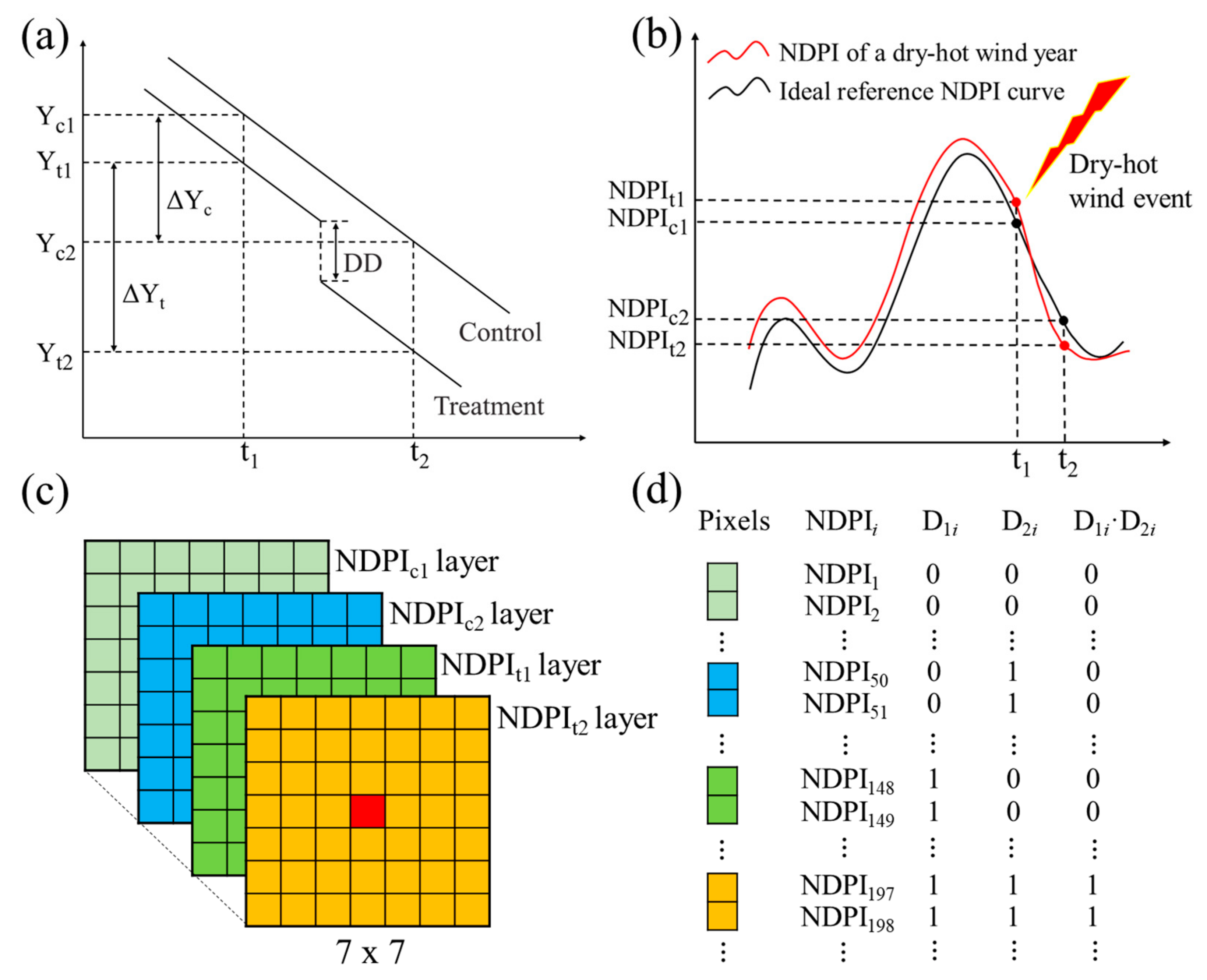
3.1. Difference-in-Differences (DID) Method

The main idea of DID is to compare the difference in outcomes (i.e., Y in Figure 3a) after and before an intervention between the affected and unaffected groups. As illustrated in Figure 3a, an external intervention (e.g., a policy) divides the samples into two groups, of which one is affected by the policy intervention (i.e., treatment group) while the other is not affected (i.e., control group).

If there is no significant difference in the trend of the observed outcomes (Y) between the treatment group and the control group (i.e., parallel trend assumption) before the external policy intervention, the change of the observed outcome (Y) after and before the policy intervention in the control group (ΔY_c, Equation (2)) can be considered as the case where the treatment group is not affected by the policy. By comparing the change of Y after and before policy intervention in treatment group (ΔY_t, Equation (3)) with that in the control group, the inherent trend in treatment group is controlled, and the independent effect of the policy (changes of Y over time and over the control group) can be isolated as DD in Equation (4)).

$$\Delta Y_c={\mathrm{Y}}_{c2}-{\mathrm{Y}}_{c1}$$

(2)

$$\Delta Y_t={\mathrm{Y}}_{t2}-{\mathrm{Y}}_{t1}$$

(3)

$$DD=\Delta Y_t-\Delta Y_c$$

(4)

The generic DID model can be expressed as

$$Y={\mathsf{\alpha }}_0+{\mathsf{\alpha }}_1{D}_1+{\mathsf{\alpha }}_2{D}_2+{\mathsf{\alpha }}_3{D}_1·D_2+\epsilon$$

(5)

where D₁ and D₂ are two dummy variables used to differentiate the treatment/control group and before/after treatment, respectively. D₁·D₂ is the cross term of these two dummy variables. α₀, α₁, α₂, and α₃ are coefficients while ε is the residual term. The values of D₁ and D₂ for the i-th observation are given by Equations (6) and (7).

$$D_1\left(i\right)=\left\{\begin{array}{l}0, observation in the control group\\ 1, observation in the treatment group\end{array}\right.$$

(6)

$$D_2\left(i\right)=\left\{\begin{array}{l}0, observation is before the intervention\\ 1, observation is after the intervention\end{array}\right.$$

(7)

Then, the coefficient of the cross term D₁·D₂ (i.e., α₃) can be solved by fitting Equation (5) by least square method, which is the unbiased estimation of DD as written in Equation (8):

$$\widehat{{\alpha }_3}= \left({\mathrm{Y}}_{t2}-{\mathrm{Y}}_{t1}\right)-\left({\mathrm{Y}}_{c2}-{\mathrm{Y}}_{c1}\right) =\Delta Y_t-\Delta Y_c=D{D}_{ }$$

(8)

3.2. Implementation of DID Method for Monitoring Dry-Hot Wind Damage

The DID method can be adapted to monitor crop response to agrometeorological hazards using remotely sensed VIs. When the occurrence of a hazard is considered as an intervention, the year when the hazard occurred can be considered as the treatment group and the hazard-free years can be treated as the control group. In this study, we use dry-hot wind as an example to illustrate the DID-based monitoring framework (Figure 3), which also can be applied to other crop types and hazards. Figure 3b–d shows the conceptual framework for implementing the DID method to monitor dry-hot wind damage to winter wheat using remotely sensed NDPI. Supposing that dry-hot wind in a given year starts at t₁ and lasts until t₂, its impact can be observed by comparing the observed NDPI curve of a wheat pixel in dry-hot wind affected year (red curve in Figure 3b) with the reference NDPI curve of the same pixel (black curve in Figure 3b). The reference NDPI curve reflects the ideal growth condition of the same pixel under the same climatic condition and phenological stages without dry-hot wind events. Accordingly, the dry-hot wind affected NDPI curve (red curve) and the ideal NDPI curve (black curve) in Figure 3b can be considered as belonging to treatment and control groups in Figure 3a, respectively. Thus, the independent effect of dry-hot wind on the winter wheat can be quantified using NDPI as:

$$\begin{gathered} D{D}_{NDPI}= \left(NDP{I}_{t2}-NDP{I}_{t1}\right) - \left(NDP{I}_{c2}-NDP{I}_{c1}\right) \\ =\Delta NDP{I}_t-\Delta NDP{I}_c \end{gathered}$$

(9)

where NDPI_t1, NDPI_t2 are values from affected NDPI curve at t₁ and t₂, and NDPI_c1, NDPI_c2 are values from the reference NDPI curve at t₁ and t₂ (Figure 3b). Following Equations (5)–(8), $D{D}_{NDPI}$ can be unbiased estimated by α₃ in fitted Equation (5).

To successfully implement the DID framework, there are three key issues that need to be addressed: (1) how to generate the reference NDPI curve in the control group, (2) how to determine NDPI values before and after dry-hot wind, and (3) how to obtain a sufficient number of samples belonging to treatment and control groups, respectively, which are needed in Equation (5) fitting.

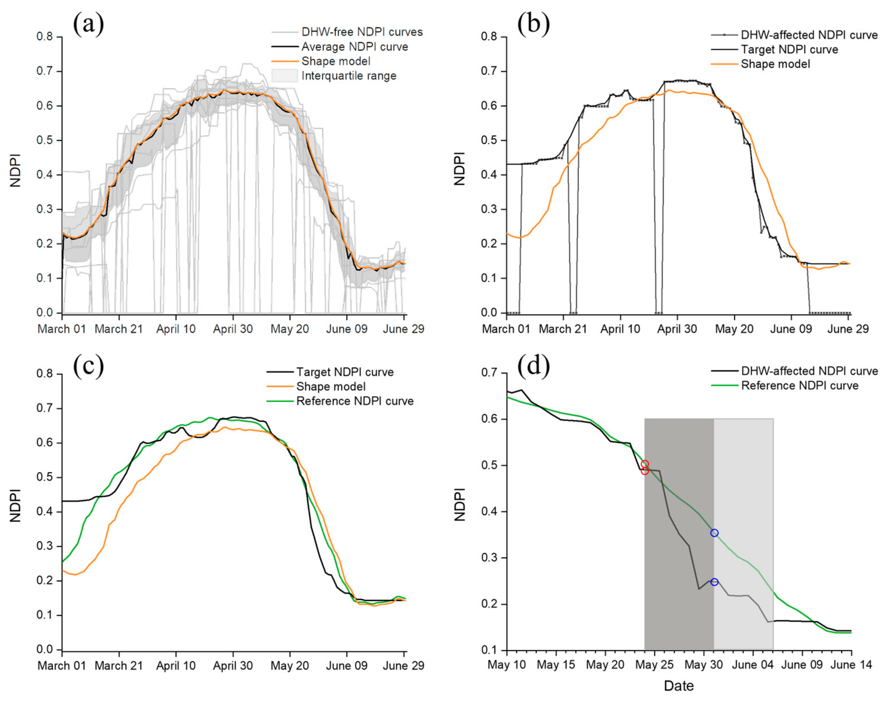
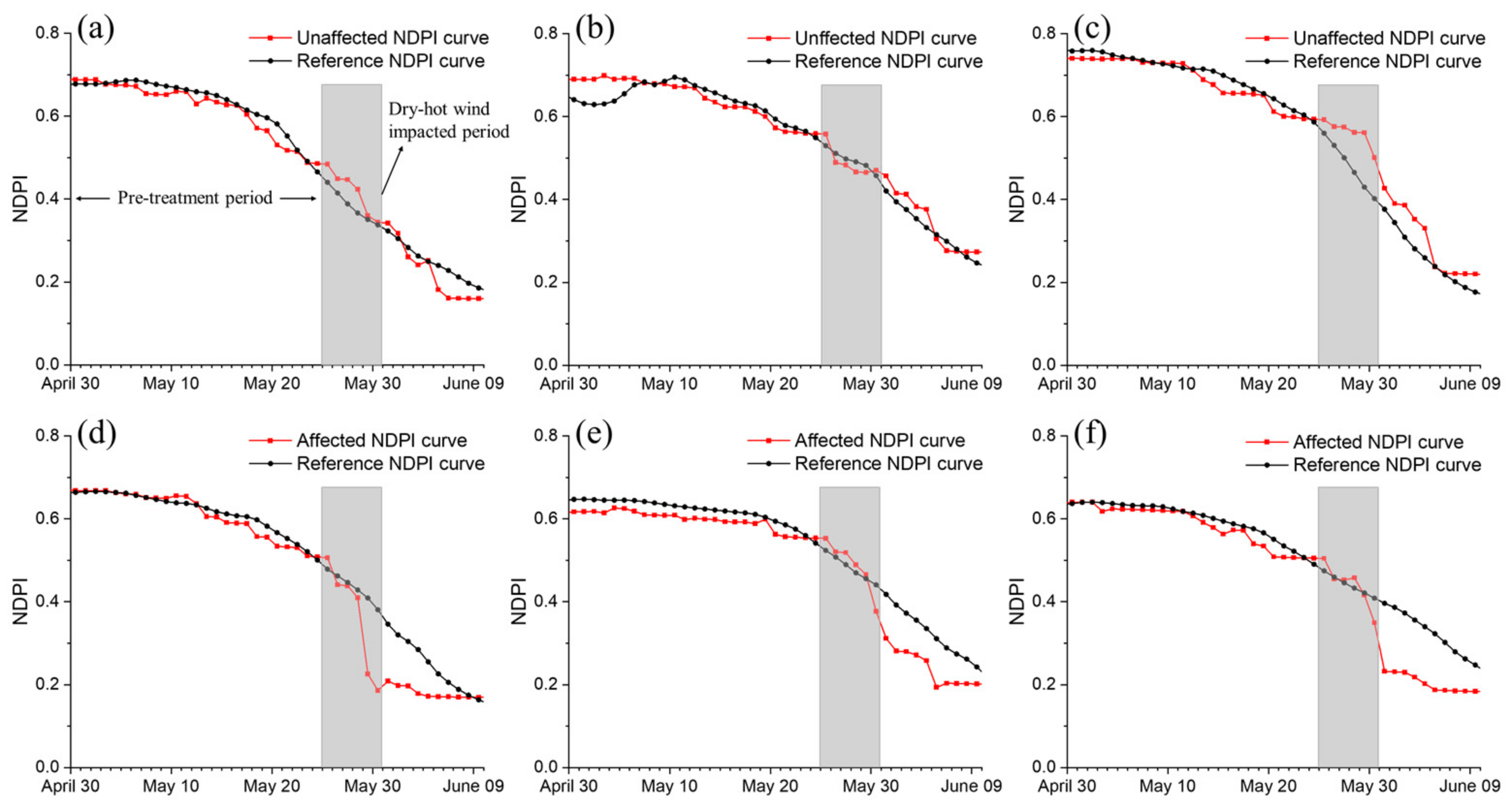
3.2.1. Generating the Reference NDPI Curve Using Shape Model Fitting

To generate the reference NDPI curve for a pixel, we first calculate the multiyear average NDPI curve (black curve in Figure 4a) using the observed NDPI of hazard-free years (gray curves in Figure 4a). To avoid outliers, only NDPI values between upper and lower quartiles are used for the multiyear average calculation. The multiyear average NDPI curve is less sensitive to missing data caused by clouds and noises comparing to any single-year NDPI curve (Figure 4a). We then apply the Savitzky–Golay (SG) filter [42,43] to further reduce possible noise and random fluctuations that may still exist in the multiyear average NDPI curve (orange curve in Figure 4a). The SG-filtered multiyear average NDPI curve is still not the optimal reference curve for a given dry-hot wind year, because it does not consider the impact of the interannual variation in climatic condition and phenological stages. To account for the interannual variations, we apply the shape model fitting (SMF) to the SG-filtered multiyear average NDPI curve [44,45,46]. SMF is effective in eliminating both phenological shifts and magnitude changes of VI curves simultaneously caused by interannual variations [5].

SMF assumes the target VI curve can be represented with a shape model adjusted by three optimized scaling parameters:

$$h\left(t\right) =s_y\times \left\{g \left(s_t\times \left(t+t_0\right)\right)\right\}$$

(10)

where function g(t) is the shape model and h(t) is the transformed VI curve as a function of time. s_y, s_t, and t₀ are three scaling parameters controlling the difference between h(t) and g(t). Here, s_t and t₀ represent phenological adjustment while s_y represents magnitude adjustment. In this study, we use the SG-filtered multiyear average NDPI curve as the shape model (i.e., g(t)). Therefore, we only need to optimize these three scaling parameters to account for the difference between the SG-filtered multiyear average NDPI curve and the transformed NDPI curve.

These three parameters are optimized by minimizing the weighted root mean square error (wRMSE, Equation (11)) between the transformed NDPI curve (green curve in Figure 4c) and the target NDPI curve, which is the SG-filtered NDPI curve of the dry-hot wind year (black curve in Figure 4c).

$$wRMSE=\sqrt{{\displaystyle \sum }_{i=1}^n{w}_i{\left(f\left(t_i\right) - h\left(t_i\right)\right)}^2}$$

(11)

In Equation (11), function f(t_i) is the target NDPI curve and h(t_i) is the transformed NDPI curve. n is the number of time steps used in curve matching, w_i is the weight of the i-th time step t_i (expressed as the day-of-year, DOY) of the NDPI curve. Different weights are given to different time steps following Equation (12) [47]:

$$D_i=\left\{\begin{array}{cc}1\hspace{1em}\hspace{1em}\hspace{1em},& t_i=t_{DHW}-1\\ \frac{1}{t_{DHW}-t_i},& t_i<t_{DHW}-1\end{array}\right.\hspace{1em}\hspace{1em}{W}_i=\frac{D_i}{{\mathrm{\Sigma }}_{i=1}^n{D}_i}$$

(12)

where $t_{DHW}$ is the date when the dry-hot wind occurred. Overall, the weight is inversely proportional to the temporal distance between t_i and $t_{DHW}-1$. We only use the NDPI curve before the dry-hot wind event for optimizing the scaling parameters to avoid the impact of the dry-hot wind. The optimized scaling parameters will be then applied to the entire SG-filtered multiyear average NDPI curve to obtain the final reference NDPI curve.

3.2.2. Determining the NDPI Values Before and After Dry-Hot Wind

The DID method requires NDPI values before and after dry-hot wind for both the treatment group and the control group. To avoid removing signals of the dry-hot wind damage on NDPI, we use the original NDPI curve of the dry-hot wind affected year (the treatment group) without applying SG filtering. However, the noise caused by cloud contamination and atmospheric effects still needs to be addressed. Thus, the highest NDPI value (red point in Figure 4d) during the duration of the dry-hot wind episode (the dark gray box in Figure 4d) is used as the observed outcome of the treatment group before the treatment. Since there is minimum noise in the reference NDPI curve, the NDPI value of the corresponding time step on the reference NDPI curve is used as the observed outcome of the control group. As for the observed outcome after the dry-hot wind, the highest NDPI value (blue point in Figure 4d) during the 3–6 days after the end of the dry-hot wind episode (the light grey box in Figure 4d) of the event year NDPI curve is selected for the treatment group. Meanwhile, the NDPI value of the corresponding time step on the reference NDPI curve is selected as the observed outcome for the control group. We use the time window of 3–6 days after the dry-hot wind event based on the assumption that the NDPI values are unlikely to recover to their previous status within this time window.

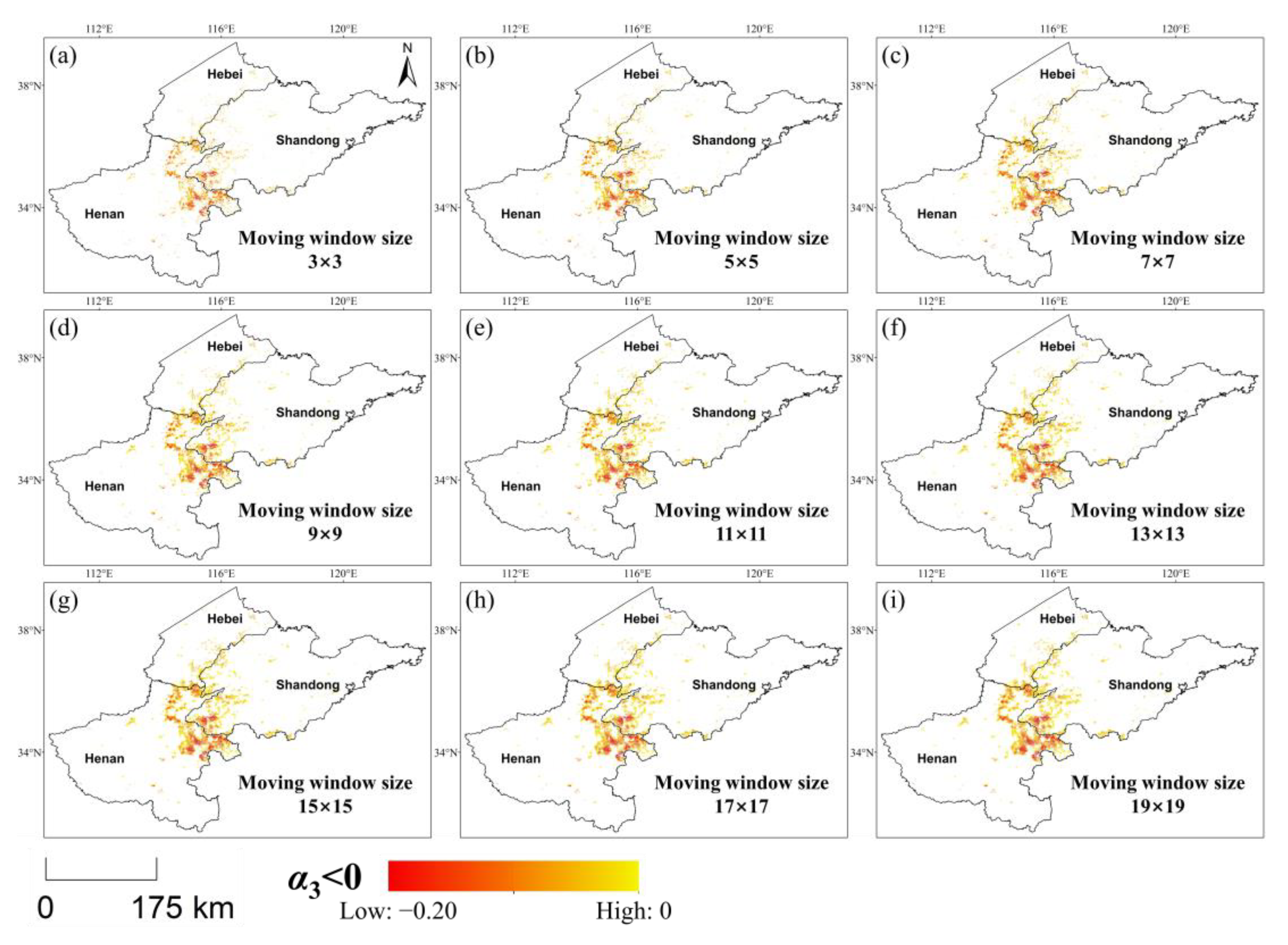
3.2.3. Using the Moving Window to Get Regression Samples

After obtaining NDPI values of the treatment and the control groups, we need to get a sufficient number of samples to fit the DID model (Equation (5)). Since the dry-hot wind typically affects a region instead of individual pixels, all pixels within a 7 × 7 moving window (3.5 × 3.5 km in MCD43A4 product) centered on the target wheat pixel (red in Figure 3c) are used for robust model fitting. The four NDPI matrices within the moving window (i.e., before/after dry-hot wind and the treatment/control group) are reassembled pixel by pixel into a tabular form as shown in Figure 3d. Then, the generic DID model can be fitted by taking NDPI as the dependent variable while D₁, D₂, and the cross term D₁·D₂ are the independent variables. The coefficient of the cross term D₁·D₂ (i.e., α₃ in Equation (5)) is the unbiased estimator of $D{D}_{NDPI}$ in Equation (9), which is used to quantify the severity of damage caused by dry-hot wind.

Generally, α₃ should be negative after the hazard, indicating the adverse effect caused by dry-hot wind on NDPI. A larger magnitude of α₃ suggests that the wheat is more seriously damaged by the dry-hot wind. Here, the Student’s t-test can be further used to exclude the pixels with nonsignificant estimates of α₃ that are likely caused by random noises (such as poor atmospheric condition and cloud contamination) rather than dry-hot wind.

4. Study Area and Data

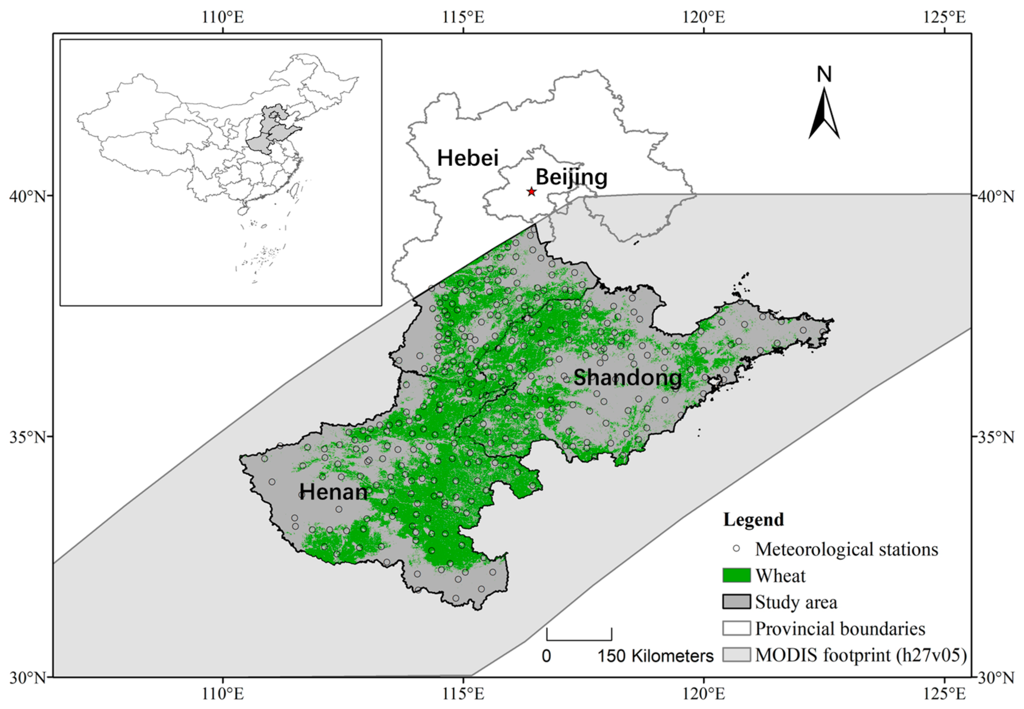
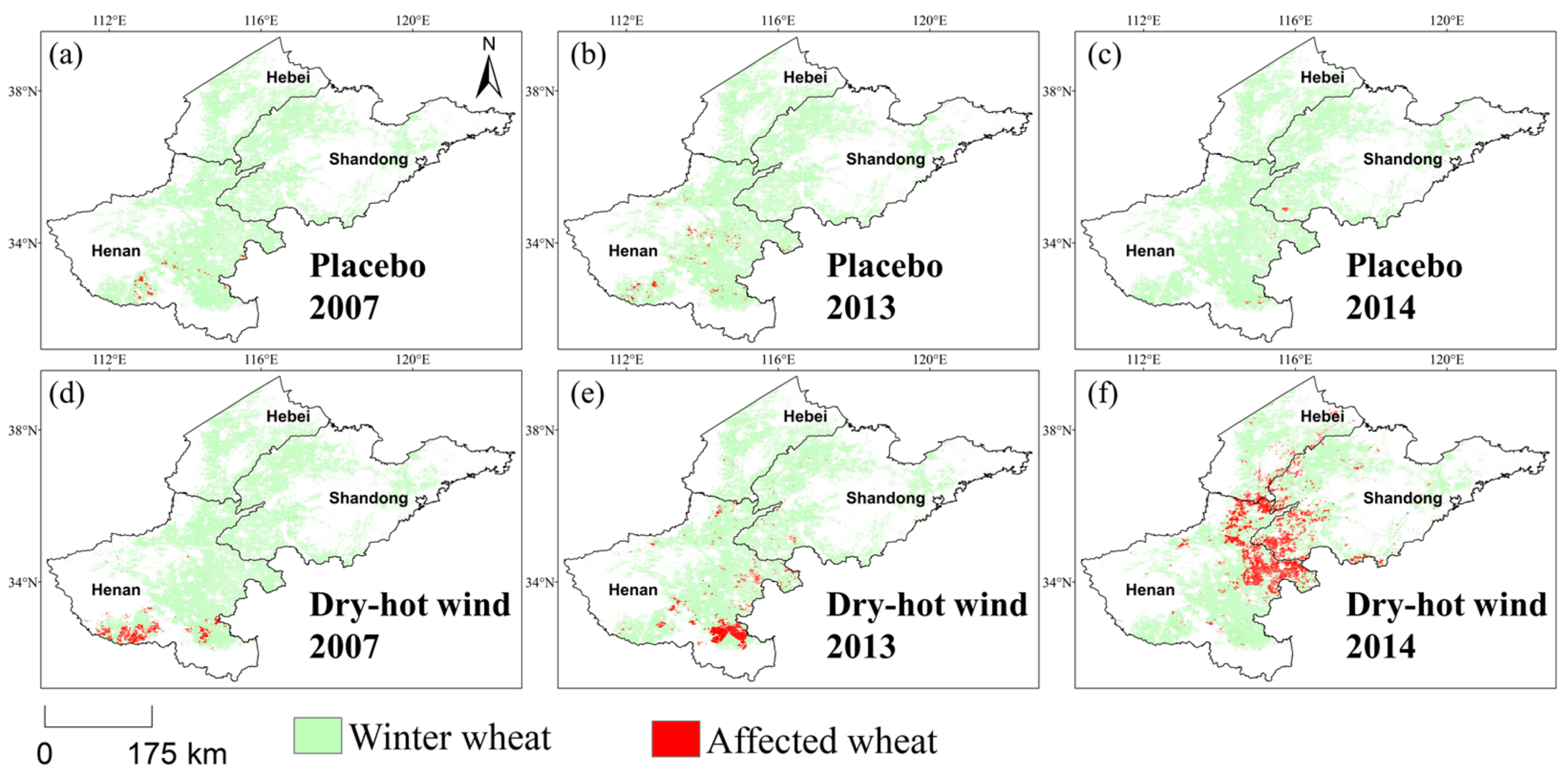
4.1. Study Area

Henan, Shandong, and Hebei are the three major winter wheat-growing provinces in China, accounting for 49.25% of the country’s wheat planting area (Third National Agricultural Census, http://olap.epsnet.com.cn/). The frequent occurrence of dry-hot wind in these provinces has become a limiting factor of stable crop yield thus affecting the national food security. It is of great importance to provide rapid monitoring and assessment of wheat damage caused by dry-hot wind in this area. As a case study, we chose the wheat planting region in these three provinces covered by a single MODIS image tile (h27v05) as the study area, which covers Henan, Shandong, and the south-central part of Hebei (Figure 5). The case study area belongs to a warm temperate monsoon climate and has relatively flat topography. The suitable climate and flat terrain make this area favorable for winter wheat cultivation [18].

4.2. Data

The MODIS nadir BRDF-adjusted daily reflectance data (MCD43A4, spatial resolution 500m) from 2002 to 2018 were downloaded from the NASA EARTHDATA website (https://earthdata.nasa.gov/). Considering the wheat growth cycle and the season when dry-hot wind typically occurs, MODIS data between March and June was used to calculate the NDPI time series in the case study. Meteorological data were collected from the Chinese Meteorological Administration (CMA) for 319 sites in the study area from 2002 to 2018. The meteorological data were used to identify dry-hot wind events according to the Meteorological Industry Standard of the People’s Republic of China: Disaster grade of dry-hot wind for wheat (QX/T 82—2019) [20]. The meteorological records were also used to select years with different severities of dry-hot wind events. For each site, the daily intensity of a dry-hot wind event was assigned value 1 (labeled as mild), 2 (moderate), or 3 (severe) based on the national standard [20]. These daily intensity levels were then summed for each dry-hot wind hazard period (usually lasting for days) to represent the meteorological intensity of the hazard at each site.

Based on the meteorological records of the study area, three dry-hot wind events occurred in mid-May 2007 (11 May–22 May, mild event), early-May 2013 (9 May–15 May, moderate event), and late May 2014 (25 May–31 May, severe event) were selected. Additionally, a 16-m crop type map provided by the Chinese Academy of Agricultural Sciences (CAAS) [48] was used to identify wheat-growing pixels in the study area. The high-resolution crop type map was aggregated to the same 500-m grid of the MODIS product.

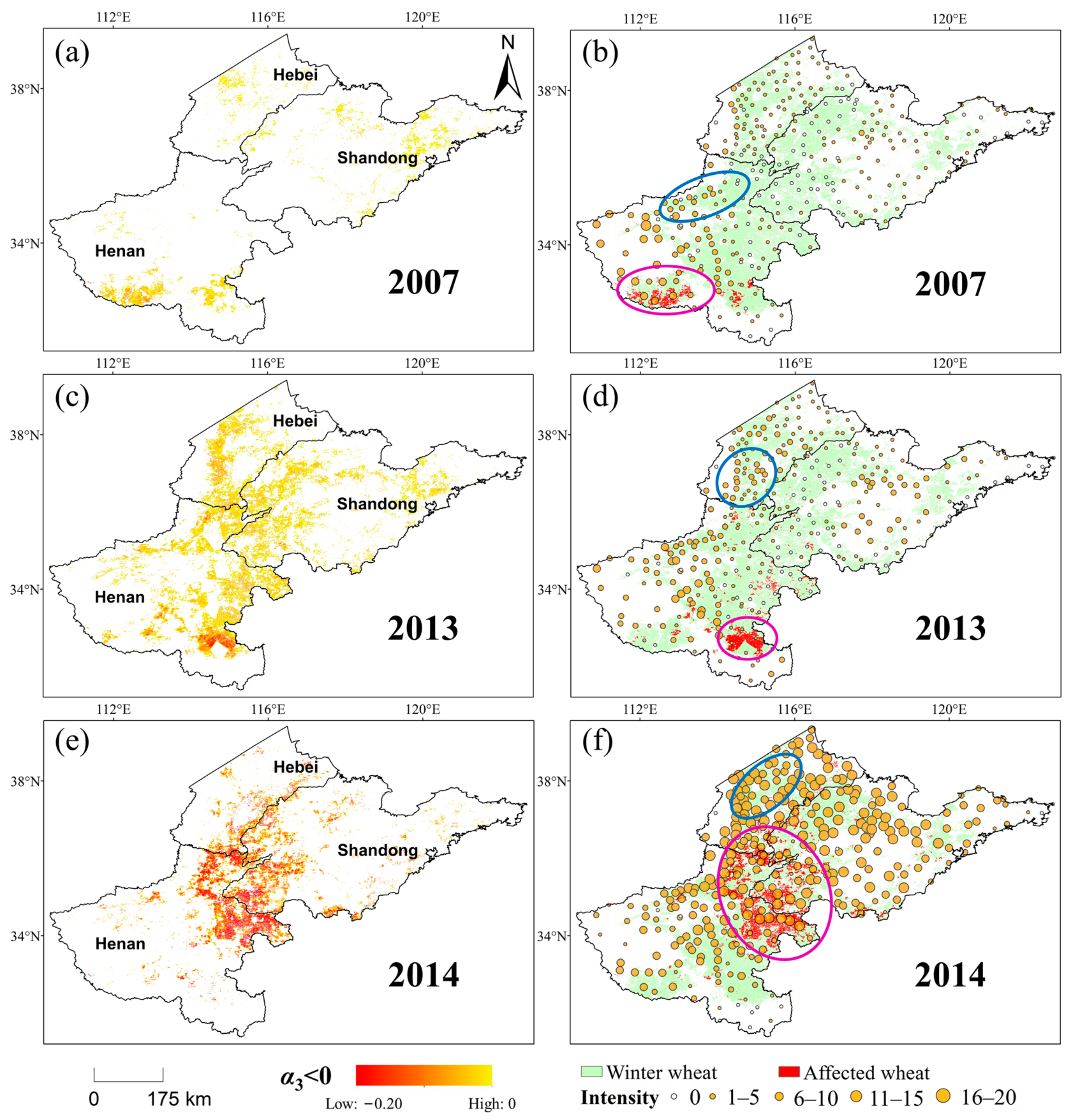
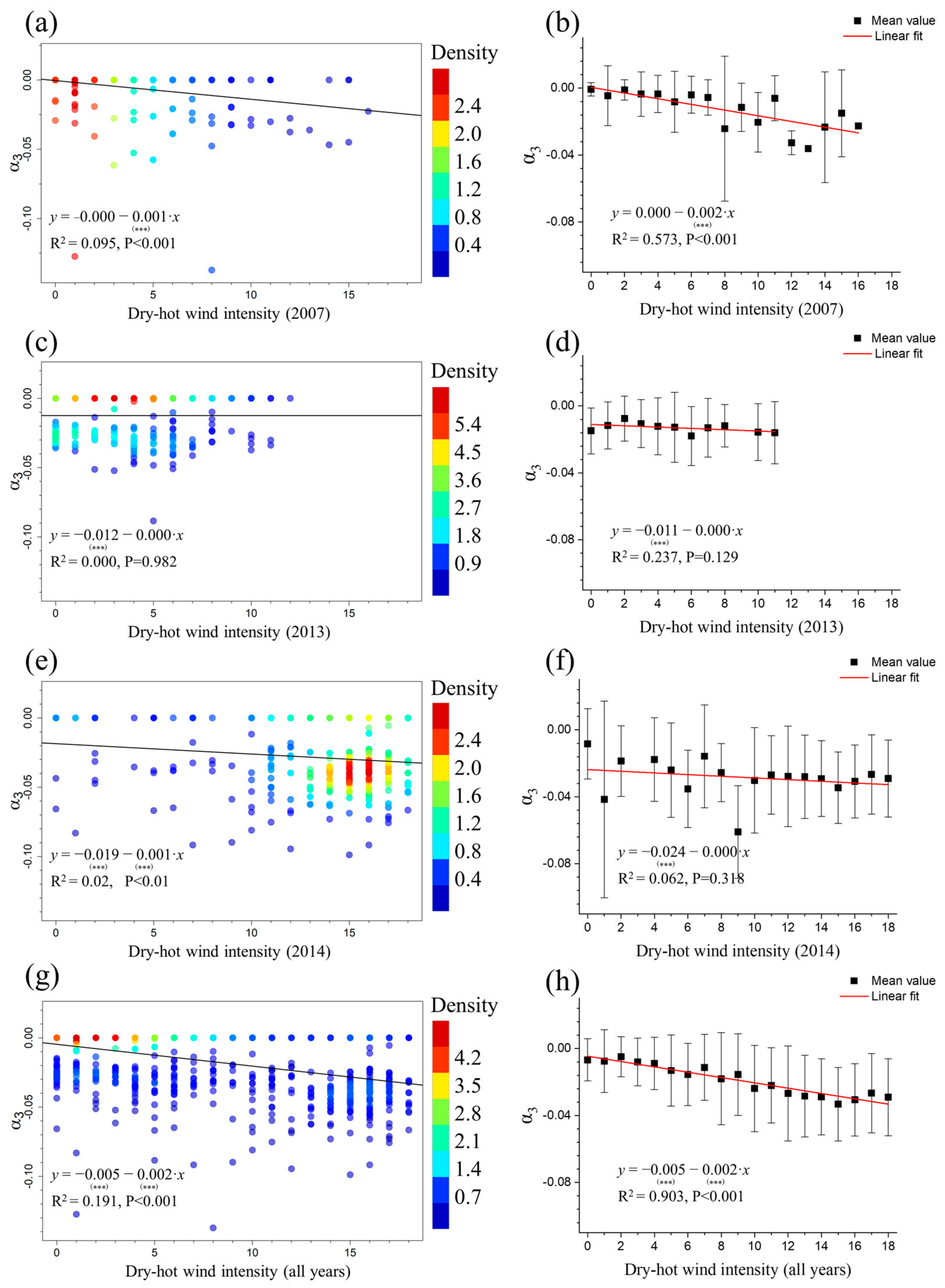
5. Case Study Results of Dry-Hot Wind Monitoring

Figure 6a,c,e shows the negative coefficient α₃ estimated from the DID-based method, which indicates the observed NDPI loss of each winter wheat pixel during dry-hot wind period in three respective years. The winter wheat pixels that show statistically significant NDPI loss (i.e., significant negative α₃, using t-test) are represented by red color, and they are considered to be dry-hot wind affected wheat in Figure 6b,d,f. Figure 6b,d,f also shows the comparison between the dry-hot wind affected wheat and the site-level intensity of dry-hot wind hazard calculated from the meteorological records.

Generally, the NDPI loss is the most serious in 2014, followed by 2013 and 2007, which is consistent with the meteorological intensity based on the site meteorological records. Additionally, the spatial distribution of the significantly affected wheat area is consistent with the distribution of sites with a higher meteorological intensity of the hazard (e.g., red circles in Figure 6b,d,f). Nonetheless, not all sites with a high meteorological intensity show statistically significant NDPI response caused by the dry-hot wind (e.g., blue circles in Figure 6b,d,f). This may be because the response of winter wheat to the dry-hot wind is not only related to the intensity of the hazard but also mitigated by soil moisture, wheat varieties, growth status, and farming interventions in response to the dry-hot wind episode. It should be noted that not all estimated NDPI loss was caused by the dry-hot wind. Other factors, such as poor atmospheric conditions, cloud contamination, and diseases and insects, could also lead to estimated NDPI loss. To ensure the robustness of further analysis, only wheat pixels with statistically significant results of α₃ (t-test, p < 0.05) were considered to be affected by dry-hot wind in this study.

Currently, there is no available field data of crop damage caused by dry-hot wind on a large scale. This is because it is difficult for wheat specialists to quantify the damage for a large area by separating the damage caused by the dry-hot wind damage and the natural wheat maturation. The lack of such field data makes it challenging to evaluate the DID-based damage estimation.

Alternatively, our results were compared with the meteorological intensity of the dry-hot wind even though the actual damage to wheat may be modulated by other factors (e.g., soil moisture, wheat varieties, growth status, and farming interventions). Although this may not be the ideal validation, it allows us to evaluate the effectiveness of our results to some extent assuming the damage to winter wheat should be generally associated with the intensity of the hazard. In other words, the estimated α₃ should be negatively correlated with the meteorological intensity of the dry-hot wind hazard.

Thus, we aggregated all statistically significant estimations of α₃ for each year within the Thiessen polygon of each meteorological site by simple average to represents the damage of winter wheat caused by dry-hot wind for each site. The aggregated estimation of damage to winter wheat was then compared with the site-level meteorological intensity of each dry-hot wind year. Figure 7 shows a significant negative correlation between the estimated damage and the event intensity for the years of 2007 (Figure 7a) and 2014 (Figure 7e), but the relationship is not significant for the year of 2013 (Figure 7c). When the data for these three years are pooled together, the relationship between the estimated damage and the event intensity appears to be stronger (Figure 7g). To further demonstrate the relationship, the mean value of the estimated damage of each site-level hazard intensity level was used (Figure 7b,d,f,h). The mean value of the estimated damage shows a stronger negative relationship with the hazard intensity when compared to site-level results, especially when the three years of data were used together. The coefficient of determination (R²) even reached 0.9 when the three-year data were aggregated (Figure 7h). These results confirmed the hypothesis that damage to winter wheat is associated with the hazard intensity thus demonstrating the effectiveness of the DID-based method for large scale monitoring to some extent.

6. Discussion

6.1. Parallel Trend Assumption

The DID method is constructed under the key parallel trend assumption, which is that the treatment and the control groups should have the same trend of the observed outcome before the treatment. As there is no available statistical test for this assumption [49], we followed other studies in econometrics using visual inspection and placebo trials to examine the validity of the parallel trend assumption [50,51]. In the visual inspection (Figure 8), the NDPI curves of the treatment group (red color) and the control group (in black) for unaffected wheat pixels (Figure 8a,b,c) exhibit good consistency of NDPI trend both in pretreatment periods and treatment periods (i.e., dry-hot wind impacted period marked by gray box). For wheat pixels with significant damage (Figure 8d,e,f), the reference NDPI curve and affected NDPI curve shows a consistent NDPI trend in the pretreatment period. During the dry-hot wind impacted period, the affected NDPI curve deviated notably from the reference NDPI curve that persists even after the dry-hot wind impacted period ended. This deviation was mainly caused by the rapidly accelerated NDPI decline due to severe dry-hot wind for the affected wheat pixels. Nonetheless, the visual inspection demonstrated that the parallel trend assumption is valid for both unaffected and affected winter wheat pixels prior to the dry-hot wind event (i.e., treatment).

To further quantitatively examine the validity of the parallel trend assumption, the placebo trials were designed for the three years used in the study (i.e., 2007, 2013, and 2014). The placebo trial is usually designed by applying the same assessment to samples without treatment. If the parallel trend assumption is true, the results of the placebo trial will be significantly different from the real assessment. In this study, the period of placebo trials was set as a period without dry-hot wind based on meteorological data before the date when the hazard occurred. The parallel trend assumption is considered valid if fewer affected wheat pixels are detected by the DID method in the placebo trial than the original DID results. Figure 9 shows that a very limited number of sparsely distributed wheat pixels were identified as affected by dry-hot wind in the placebo trials, which is significantly different from the DID-based assessment for the actual dry-hot wind event. The limited number of affected wheat pixels detected in the placebo trials is likely related to the rapid decrease of NDPI caused by random noises or other agricultural hazards (e.g., cloud contamination, drought, or pests, etc.).

Both the visual inspection and the placebo trials confirmed that the parallel trend assumption is valid for this case study using the DID-based framework to evaluate winter wheat damage caused by the dry-hot wind. We recommend that users who are interested in applying this framework to different applications should examine the validity of the parallel trend assumption using similar methods for their applications.

6.2. Sensitivity to Moving Window Size

In the proposed DID framework, we used a 7 × 7 moving window surrounding the target wheat pixel to determine which samples (i.e., wheat pixels) were used to estimate the coefficient α₃ based on the assumption that the dry-hot wind plays a similar role in a local region with similar local environmental conditions. We tested the sensitivity of the framework to the moving window size to determine the proper size by varying the window size between 3 × 3 pixels (i.e., 2.25 km²) to 19 × 19 pixels (i.e., 90.25 km²) with an increment of two MODIS pixels.

Here we only used the dry-hot wind event in 2014 as an example. Figure 10 shows the monitoring results using different window sizes, which are almost identical in the spatial distribution. This similar spatial distribution suggests that the DID-based framework is not sensitive to the moving window size. When the moving window size is limited to 3 × 3 and 5 × 5 pixels, fewer damaged wheat pixels were identified than the results when a larger window size was used. However, this difference is not noticeable when the window size is larger than 7 × 7 pixels. To ensure sufficient samples for robust model fitting, we thus chose 7 × 7 pixels as the moving window for this study. It should be noted that future research should examine a more efficient strategy to determine the optimum window size for the DID-based framework instead of this trial-and-error method which can be computationally intensive.

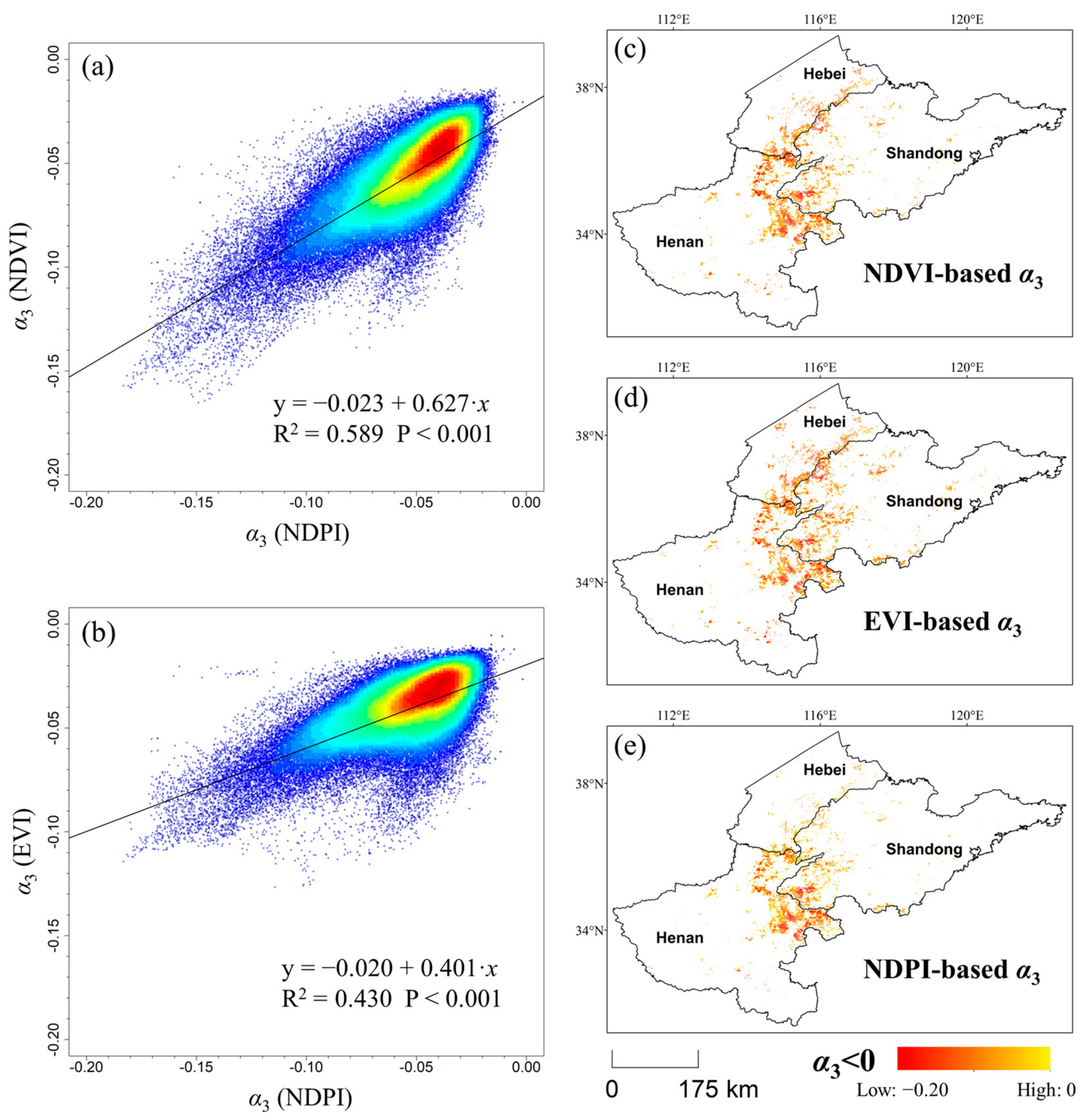
6.3. Applicability of DID Method to Different Vegetation Indices

As mentioned in Section 2.2, NDPI is more suited for monitoring dry-hot wind damage to winter wheat thanks to the introduction of SWIR band which is sensitive to plant leaf water content. However, NDPI cannot be calculated using some high-resolution remotely sensed data without the SWIR band for fine-scale monitoring. Thus, we tested whether the DID method is equally applicable by using other vegetation indices that do not require the SWIR band (i.e., NDVI and EVI) to monitor winter wheat response to the dry-hot wind. Figure 11 shows the scatterplots of estimated a₃ using NDVI and EVI [38,39] compared against the estimated a₃ using NDPI and the spatial distribution of the statistically significant negative a₃ estimated using all three VI for the year of 2014. There is a better agreement between the NDVI-based results and the NDPI-based results, with the R² approaching to 0.6 (Figure 11a) compared with that of EVI-based results (R² = 0.43) (Figure 11b). Results using three different VIs show a similar spatial pattern of the detected wheat damage, although the EVI-based result appears to be more dispersed. Therefore, in cases when NDPI is not available, NDVI can be used as an alternative VI for assessing dry-hot wind damage to winter wheat.

6.4. Advantages and Limitations of the DID Framework

Dry-hot wind hazards can impose detrimental impacts on wheat growth and yield. In this paper, we proposed a general DID framework and applied it to quantify the dry-hot wind damage to winter wheat. The main advantage of this method is that it can effectively isolate the independent impact of the dry-hot wind from the mixed signals observed in the inherent downward trend of the NDPI curve due to the wheat maturation process. To the best of our knowledge, the separation of independent effects is not possible with the existing methods using remotely sensed data on a large scale.

There are three key steps to implement the DID framework for monitoring the winter wheat response to dry-hot winds. The first step is to construct a reference NDPI curve for the control group using the multiyear average NDPI curve (derived from hazard-free years) and then adjusted using the shape model fitting (SMF) method. This process allowed us to take full advantage of the historical data to robustly account for the impacts related to interannual variations of climatic conditions and phenological stages on the reference NDPI curve. Additionally, it ensures the validity of the parallel trend assumption between the reference NDPI curve (the control group) and the observed NDPI curve of the dry-hot wind year (the treatment group). In the second step, the time steps with the largest NDPI value were chosen during the period of dry-hot wind hazard and during the 3–6 days after the end of the dry-hot wind, respectively, to avoid potential impact from random noise in the data. The third step uses a 7 × 7 pixel moving window to fully utilize the spatial information from adjacent pixels to estimate the impact. It also allows for a statistical significance test to ensure robust estimation of the impact that is caused by the dry-hot wind. In our case study, only pixels with statistically significant estimations were considered to be caused by the dry-hot wind. The statistical test using the moving window allowed us to filter out pixels with similar NDPI reduction that may be caused by data noise or other factors. Additionally, the DID framework has been shown effective using both NDPI and NDVI for monitoring the impact of dry-hot wind to winter wheat, suggesting the flexibility of such a framework. The general DID framework can also be applied to other crop types and hazard events with careful adjustment.

However, the newly proposed method also has its limitations. As multiple agricultural hazards (e.g., drought, diseases, and pests, etc.) may cause NDPI to decrease like dry-hot wind, the prior knowledge of the dry-hot wind hazard occurrence (e.g., start and end dates) extracted from the meteorological data are required as auxiliary data before applying the DID framework. Moreover, if a dry-hot wind event coincides or overlaps with other agricultural hazards, the NDPI decrease obtained from the DID based method (i.e., a₃) reflects the compounding impacts rather than the independent impact of the dry-hot wind event. It is difficult to isolate the individual contribution of the dry-hot wind from other hazards unless a remote sensing-based indicator that responds only to the dry-hot wind is established in the future. Last but not least, we used dry-hot wind intensity extracted from the meteorological data to evaluate our results because there is currently no available field data on a large scale to evaluate the impacts caused by the dry-hot wind. Although we found good agreement between dry-hot wind intensity and DID-based damage estimation, it should be noted that this evaluation cannot replace the direct validation against the field survey data when such data is available. To address this issue, appropriate field data will need to be collected before and after a dry-hot wind event in future work. With the rapid development of mobile devices, using mobile phone-based software and citizen science or volunteer geoinformation system could be a potential solution to fill the field data gap.

7. Conclusions

In this study, we presented a general DID framework for monitoring crop response to agrometeorological hazards with satellite data and applied it to quantify the dry-hot wind damage to winter wheat in northern China. The main advantage of this method is that it can control the intrinsic changing trend of the observed outcome (i.e., NDPI), thus allowing for effective isolation of the observed outcome change (i.e., NDPI reduction) caused independently by the hazard event (i.e., dry-hot wind hazard). In the case study of dry-hot wind damage monitoring, there are three key steps in implementing the proposed DID framework including (1) generating the reference NDPI curve, (2) determining NDPI values before and after the dry-hot wind event, and (3) using a moving window to use spatial information to robustly estimate the damage. To generate the reference NDPI curve with the similar environmental conditions of the hazard year, the SMF method was used to account for the impact of the interannual variations of climatic conditions and phenological stages on the NDPI curve. It also ensures the validity of the parallel trend assumption between the reference NDPI curve (the control group) and the hazard year NDPI curve (the treatment group). Through this series of processing, both the historical data and the spatial information within a local region can be fully utilized. Moreover, the proposed DID-based framework is very flexible and can be easily extended to other natural hazards and crop types with proper adjustment. We indirectly evaluated the results in the case study of winter wheat damage caused by the dry-hot wind by comparing with the intensity level of the dry-hot wind events because of the lack of field data to directly validate the results. The notable relationship (R² = 0.903, p < 0.001) between the intensity of the dry-hot wind and the estimated damage of the dry-hot wind demonstrated the effectiveness of the newly proposed DID framework. However, future work is still needed to use actual field data on a large scale to evaluate the DID framework.

References

1. IPCC. Summary for Policymakers SPM. IPCC 2019. [Google Scholar] [CrossRef] [Green Version]
2. Huang, J.; Han, D. Meta-analysis of influential factors on crop yield estimation by remote sensing. Int. J. Remote Sens. 2014, 35, 2267–2295. [Google Scholar] [CrossRef]
3. Kogan, F.N. Remote sensing of weather impacts on vegetation in non-homogeneous areas. Int. J. Remote Sens. 1990, 11, 1405–1419. [Google Scholar] [CrossRef]
4. Tucker, C.; Vanpraet, C.; Boerwinkel, E.; Gaston, A. Satellite remote sensing of total dry matter production in the Senegalese Sahel. Remote Sens. Environ. 1983, 13, 461–474. [Google Scholar] [CrossRef]
5. Wang, S.; Chen, J.; Rao, Y.; Liu, L.; Wang, W.; Dong, Q. Response of winter wheat to spring frost from a remote sensing perspective: Damage estimation and influential factors. ISPRS J. Photogramm. Remote Sens. 2020, 168, 221–235. [Google Scholar] [CrossRef]
6. Wright, J.; Lillesand, T.M.; Kiefer, R.W. Remote Sensing and Image Interpretation. Geogr. J. 1980, 146, 448. [Google Scholar] [CrossRef]
7. Jackson, R.; Pinter, P.; Reginato, R.; Idso, S. Detection and Evaluation of Plant Stresses for Crop Management Decisions. IEEE Trans. Geosci. Remote Sens. 1986, GE-24, 99–106. [Google Scholar] [CrossRef]
8. Chong, Y.M.; SivaKumar, B.; Ahmad, H.M. Detecting and Monitoring Plant Nutrient Stress Using Remote Sensing Approaches: A Review. Asian J. Plant Sci. 2017, 16, 1–8. [Google Scholar] [CrossRef]
9. Maes, W.H.; Steppe, K. Estimating evapotranspiration and drought stress with ground-based thermal remote sensing in agriculture: A review. J. Exp. Bot. 2012, 63, 4671–4712. [Google Scholar] [CrossRef] [PubMed] [Green Version]
10. Menzel, A.; Helm, R.; Zang, C. Patterns of late spring frost leaf damage and recovery in a European beech (Fagus sylvatica L.) stand in south-eastern Germany based on repeated digital photographs. Front. Plant Sci. 2015, 6, 110. [Google Scholar] [CrossRef] [Green Version]
11. Nolè, A.; Rita, A.; Ferrara, A.M.S.; Borghetti, M. Effects of a large-scale late spring frost on a beech (Fagus sylvatica L.) dominated Mediterranean mountain forest derived from the spatio-temporal variations of NDVI. Ann. For. Sci. 2018, 75, 83. [Google Scholar] [CrossRef] [Green Version]
12. Allevato, E.; Saulino, L.; Cesarano, G.; Chirico, G.B.; D’Urso, G.; Falanga Bolognesi, S.; Rita, A.; Rossi, S.; Saracino, A.; Bonanomi, G. Canopy damage by spring frost in European beech along the Apennines: Effect of latitude, altitude and aspect. Remote Sens. Environ. 2019, 225, 431–440. [Google Scholar] [CrossRef]
13. Abadie, A. Semiparametric Difference-in-Differences Estimators. Rev. Econ. Stud. 2005, 72, 1–19. [Google Scholar] [CrossRef]
14. Ashenfelter, O. Estimating the Effect of Training Programs on Earnings. Rev. Econ. Stat. 1978, 60, 47. [Google Scholar] [CrossRef]
15. Ashenfelter, O.; Card, D. Using the Longitudinal Structure of Earnings to Estimate the Effect of Training Programs. Rev. Econ. Stat. 1985, 67, 648. [Google Scholar] [CrossRef]
16. Jiménez, J.L.; Perdiguero, J. Difference-In-Difference. In Encyclopedia of Law and Economics; Marciano, A., Ramello, G.B., Eds.; Springer: New York, NY, USA, 2017; Volume 52, pp. 1–4. ISBN 978-1-4614-7883-6. [Google Scholar]
17. Bertrand, M.; Duflo, E.; Mullainathan, S. How Much Should We Trust Differences-In-Differences Estimates? Q. J. Econ. 2004, 119, 249–275. [Google Scholar] [CrossRef] [Green Version]
18. Jin, S. Wheat in China; China Agricultural Press: Beijing, China, 1996. [Google Scholar]
19. Xiao, L.; Liu, L.; Asseng, S.; Xia, Y.; Tang, L.; Liu, B.; Cao, W.; Zhu, Y. Estimating spring frost and its impact on yield across winter wheat in China. Agric. For. Meteorol. 2018, 260–261, 154–164. [Google Scholar] [CrossRef]
20. China Meteorological Administration. Meteorological Industry Standard of the People’s Republic of China: Disaster Grade of Dry-Hot Wind for Wheat (QX/T 82-2019); China Meteorological Administration: Beijing, China, 2019. [Google Scholar]
21. Al-Khatib, K.; Paulsen, G.M. Mode of high temperature injury to wheat during grain development. Physiol. Plant. 1984, 61, 363–368. [Google Scholar] [CrossRef]
22. Chen, Y.; Zhang, Z.; Tao, F.; Palosuo, T.; Rötter, R.P. Impacts of heat stress on leaf area index and growth duration of winter wheat in the North China Plain. F. Crop. Res. 2018, 222, 230–237. [Google Scholar] [CrossRef] [Green Version]
23. Asseng, S.; Ewert, F.; Martre, P.; Rötter, R.P.; Lobell, D.B.; Cammarano, D.; Kimball, B.A.; Ottman, M.J.; Wall, G.W.; White, J.W.; et al. Rising temperatures reduce global wheat production. Nat. Clim. Chang. 2015, 5, 143–147. [Google Scholar] [CrossRef]
24. Farooq, M.; Bramley, H.; Palta, J.A.; Siddique, K.H.M. Heat Stress in Wheat during Reproductive and Grain-Filling Phases. CRC. Crit. Rev. Plant Sci. 2011, 30, 491–507. [Google Scholar] [CrossRef]
25. Ortiz, R.; Sayre, K.D.; Govaerts, B.; Gupta, R.; Subbarao, G.V.; Ban, T.; Hodson, D.; Dixon, J.M.; Iván Ortiz-Monasterio, J.; Reynolds, M. Climate change: Can wheat beat the heat? Agric. Ecosyst. Environ. 2008, 126, 46–58. [Google Scholar] [CrossRef]
26. Gouache, D.; Le Bris, X.; Bogard, M.; Deudon, O.; Pagé, C.; Gate, P. Evaluating agronomic adaptation options to increasing heat stress under climate change during wheat grain filling in France. Eur. J. Agron. 2012, 39, 62–70. [Google Scholar] [CrossRef]
27. Moore, F.C.; Lobell, D.B. Adaptation potential of European agriculture in response to climate change. Nat. Clim. Chang. 2014, 4, 610–614. [Google Scholar] [CrossRef]
28. Song, L.; Guanter, L.; Guan, K.; You, L.; Huete, A.; Ju, W.; Zhang, Y. Satellite sun-induced chlorophyll fluorescence detects early response of winter wheat to heat stress in the Indian Indo-Gangetic Plains. Glob. Chang. Biol. 2018, 24, 4023–4037. [Google Scholar] [CrossRef] [Green Version]
29. Barlow, K.M.; Christy, B.P.; O’Leary, G.J.; Riffkin, P.A.; Nuttall, J.G. Simulating the impact of extreme heat and frost events on wheat crop production: A review. F. Crop. Res. 2015, 171, 109–119. [Google Scholar] [CrossRef] [Green Version]
30. Challinor, A.J.; Wheeler, T.R.; Craufurd, P.Q.; Slingo, J.M. Simulation of the impact of high temperature stress on annual crop yields. Agric. For. Meteorol. 2005, 135, 180–189. [Google Scholar] [CrossRef] [Green Version]
31. Kussul, N.; Skakun, S.; Shelestov, A.; Kravchenko, O.; Gallego, J.F.; Kussul, O. Crop area estimation in Ukraine using satellite data within the MARS project. In Proceedings of the 2012 IEEE International Geoscience and Remote Sensing Symposium, Munich, Germany, 22–27 July 2012; pp. 3756–3759. [Google Scholar]
32. Hering, D.; Carvalho, L.; Argillier, C.; Beklioglu, M.; Borja, A.; Cardoso, A.C.; Duel, H.; Ferreira, T.; Globevnik, L.; Hanganu, J.; et al. Managing aquatic ecosystems and water resources under multiple stress—An introduction to the MARS project. Sci. Total Environ. 2015, 503–504, 10–21. [Google Scholar] [CrossRef]
33. Hochman, Z.; van Rees, H.; Carberry, P.S.; Hunt, J.R.; McCown, R.L.; Gartmann, A.; Holzworth, D.; van Rees, S.; Dalgliesh, N.P.; Long, W.; et al. Re-inventing model-based decision support with Australian dryland farmers. 4. Yield Prophet® helps farmers monitor and manage crops in a variable climate. Crop Pasture Sci. 2009, 60, 1057. [Google Scholar] [CrossRef] [Green Version]
34. Droutsas, I.; Challinor, A.J.; Swiderski, M.; Semenov, M.A. New modelling technique for improving crop model performance—Application to the GLAM model. Environ. Model. Softw. 2019, 118, 187–200. [Google Scholar] [CrossRef] [Green Version]
35. Akter, N.; Rafiqul Islam, M. Heat stress effects and management in wheat. A review. Agron. Sustain. Dev. 2017, 37, 37. [Google Scholar] [CrossRef]
36. Liu, J.; Zhang, X.; Ma, G.; Cao, N.; Ma, L. Analysis on spring wheat spectrum characteristics influenced by dry-hot wind in Ningxia. Trans. Chin. Soc. Agric. Eng. 2012, 28, 189–199. [Google Scholar]
37. Li, Y.; Chen, H.; Wang, X.; Zhang, H. Prediction of Winter Wheat Yield Loss Caused by Dry-hot Wind Based on Remote Sensing. In Proceedings of the 32nd Conference on Hydrology, Austin, TX, USA, 7–11 January 2018. [Google Scholar]
38. Tucker, C.J. Red and photographic infrared linear combinations for monitoring vegetation. Remote Sens. Environ. 1979, 8, 127–150. [Google Scholar] [CrossRef] [Green Version]
39. Huete, A.; Didan, K.; Miura, T.; Rodriguez, E.; Gao, X.; Ferreira, L. Overview of the radiometric and biophysical performance of the MODIS vegetation indices. Remote Sens. Environ. 2002, 83, 195–213. [Google Scholar] [CrossRef]
40. Wang, C.; Chen, J.; Wu, J.; Tang, Y.; Shi, P.; Black, T.A.; Zhu, K. A snow-free vegetation index for improved monitoring of vegetation spring green-up date in deciduous ecosystems. Remote Sens. Environ. 2017, 196, 1–12. [Google Scholar] [CrossRef]
41. Cao, R.; Feng, Y.; Liu, X.; Shen, M.; Zhou, J. Uncertainty of Vegetation Green-Up Date Estimated from Vegetation Indices Due to Snowmelt at Northern Middle and High Latitudes. Remote Sens. 2020, 12, 190. [Google Scholar] [CrossRef] [Green Version]
42. Chen, J.; Jönsson, P.; Tamura, M.; Gu, Z.; Matsushita, B.; Eklundh, L. A simple method for reconstructing a high-quality NDVI time-series data set based on the Savitzky–Golay filter. Remote Sens. Environ. 2004, 91, 332–344. [Google Scholar] [CrossRef]
43. Cao, R.; Chen, Y.; Shen, M.; Chen, J.; Zhou, J.; Wang, C.; Yang, W. A simple method to improve the quality of NDVI time-series data by integrating spatiotemporal information with the Savitzky-Golay filter. Remote Sens. Environ. 2018, 217, 244–257. [Google Scholar] [CrossRef]
44. Sakamoto, T.; Wardlow, B.D.; Gitelson, A.A.; Verma, S.B.; Suyker, A.E.; Arkebauer, T.J. A Two-Step Filtering approach for detecting maize and soybean phenology with time-series MODIS data. Remote Sens. Environ. 2010, 114, 2146–2159. [Google Scholar] [CrossRef]
45. Sakamoto, T.; Gitelson, A.A.; Arkebauer, T.J. MODIS-based corn grain yield estimation model incorporating crop phenology information. Remote Sens. Environ. 2013, 131, 215–231. [Google Scholar] [CrossRef]
46. Sakamoto, T. Refined shape model fitting methods for detecting various types of phenological information on major U.S. crops. ISPRS J. Photogramm. Remote Sens. 2018, 138, 176–192. [Google Scholar] [CrossRef]
47. Chen, J.; Rao, Y.; Shen, M.; Wang, C.; Zhou, Y.; Ma, L.; Tang, Y.; Yang, X. A Simple Method for Detecting Phenological Change From Time Series of Vegetation Index. IEEE Trans. Geosci. Remote Sens. 2016, 54, 3436–3449. [Google Scholar] [CrossRef]
48. Tang, H.; Zhou, Q.; Liu, J.; Li, Z.; Wu, W. Wheat Mapping Using High Resolution Remote Sensing Data; Science Press of China: Beijing, China, 2016. [Google Scholar]
49. Wing, C.; Simon, K.; Bello-Gomez, R.A. Designing Difference in Difference Studies: Best Practices for Public Health Policy Research. Annu. Rev. Public Health 2018, 39, 453–469. [Google Scholar] [CrossRef] [PubMed] [Green Version]
50. Kaestner, R.; Garrett, B.; Chen, J.; Gangopadhyaya, A.; Fleming, C. Effects of ACA Medicaid Expansions on Health Insurance Coverage and Labor Supply. J. Policy Anal. Manag. 2017, 36, 608–642. [Google Scholar] [CrossRef] [PubMed]
51. Telles, S.; Reddy, S.K.; Nagendra, H.R. Summary for Policymakers. In Climate Change 2013—The Physical Science Basis; Intergovernmental Panel on Climate Change, Ed.; Cambridge University Press: Cambridge, UK, 2019; Volume 53, pp. 1–30. ISBN 9788578110796. [Google Scholar]
Figure 1. The growth cycle of winter wheat represented by the time series of remotely sensed normalized difference vegetation index (NDVI, green curve) and the relevant hazards that may occur at different crop growth stages. The numbers in parentheses represent the number of relevant published papers in the Web of Science Core Collection for the corresponding hazards.
Remotesensing 13 00482 g001
Figure 2. The response of MODIS BRDF-adjusted spectral reflectance (MCD43A4) and VIs to the dry-hot wind. During this period, winter wheat is in grain-filling period. (a,b) shows the response to a mild dry-hot wind event, (c,d) exhibits the response to a moderate dry-hot wind event, and (e,f) represents the response to a severe dry-hot wind event. The gray areas represent the duration of the dry-hot wind events.
Remotesensing 13 00482 g002
Figure 3. The conceptual framework of the DID-based method to monitor dry-hot wind damage to winter wheat. (a) illustrates the basic principle of DID model; (b) is a schematic diagram of using DID model to monitor dry-hot wind disaster for winter wheat; (c) represents four NDPI matrices within a 7 × 7 moving window centered on a target wheat pixel (i.e., before/after dry-hot wind and the treatment/control group); (d) is tabular form of wheat pixels reassembled pixel by pixel from the four NDPI matrices in (c). These pixels are then used for DID model fitting.
Remotesensing 13 00482 g003
Figure 4. The shape model fitting method to generate the reference NDPI curve (DHW in legend represents dry-hot wind). (a) illustrates how the shape model is generated using the multiyear NDPI curves. Interquartile range is represented by light gray-shaded areas in (a); (b) shows the difference between the shape model and the target NDPI curve; (c) shows the process of generating the reference NDPI curve using shape model fitting method; (d) illustrates how to determine the NDPI values before and after the occurrence of dry-hot wind from the dry-hot wind affected NDPI curve and the reference NDPI curve. Dark gray box in (d) represents the duration of dry-hot wind episode and light gray box represents 6 days after the end of the dry-hot wind episode.
Remotesensing 13 00482 g004
Figure 5. Study area and locations of meteorological stations.
Remotesensing 13 00482 g005
Figure 6. The NDPI loss derived from the DID-based method and the corresponding meteorological intensity of dry-hot wind hazard for the year of 2007 (mild, (a,b)), 2013 (moderate, (c,d)), and 2014 (severe, (e,f)). The green shaded pixels in (b,d,f) represent the wheat-growing area based on the resampled crop type map. The area marked by red color in the second column shows the area with statistically significant NDPI loss (i.e., significant negative α3, using t-test) based on the DID method. Each point in the second column represents a site with the size corresponding to the intensity of dry-hot wind for that year calculated from the meteorological records. Red circles in (b,d,f) indicate that the spatial distribution of the significantly affected wheat area is consistent with the distribution of sites with a higher meteorological intensity of the hazard. However, blue circles indicate that their spatial distribution is inconsistent.
Remotesensing 13 00482 g006
Figure 7. The comparison between the damage to winter wheat estimated by the DID-based method and the meteorological intensity of dry-hot wind hazards (a,b): 2007, (c,d): 2013, (e,f): 2014, (g,h): all three years; the colors in subplots (a,c,e), and (g) represent data point density estimated by kde2d function in R. They are related to the number of days with the same dry-hot wind intensity and similar α3 value).
Remotesensing 13 00482 g007
Figure 8. Visual inspection of the parallel trend assumption. The NDPI curves of three dry-hot wind years (a,d): 2007; (b,e): 2013; (c,f): 2014) are in red and their corresponding reference curves are in black. Typical pixels unaffected by dry-hot wind are shown as the first row (a,b,c) while typical pixels affected by dry-hot wind are shown as the second row (d,e,f). The dry-hot wind impacted periods are marked by a gray box.
Remotesensing 13 00482 g008
Figure 9. Results of the placebo trial of the three years used in this study. The first row is the placebo trial results (a,b,c) and the second row is the actual dry-hot wind monitoring results (d,e,f).
Remotesensing 13 00482 g009
Figure 10. The monitoring results for the year 2014 using different moving window sizes. (a)–(i) are the re-sults of using different window sizes ranging from 3 × 3 pixels to 19 × 19 pixels with the increment of two pixels.
Remotesensing 13 00482 g010
Figure 11. The scatterplots of estimated a3 using NDVI and EVI against the estimated a3 using NDPI for the year of 2014 (a,b) and the spatial distribution of statistically significant negative a3 estimation using NDVI (c), EVI (d), and NDPI (e).
Remotesensing 13 00482 g011