Abstract
High-quality Normalized Difference Vegetation Index (NDVI) time series are essential in studying vegetation phenology, dynamic monitoring, and global change. Gap filling is the most important issue in reconstructing NDVI time series from satellites with high spatial resolution, e.g., the Landsat series and Chinese GaoFen-1/6 series. Due to the sparse revisit frequencies of high-resolution satellites, traditional reconstruction approaches face the challenge of dealing with large gaps in raw NDVI time series data. In this paper, a climate incorporated gap-filling (CGF) method is proposed for the reconstruction of Landsat historical NDVI time series data. The CGF model considers the relationship of the NDVI time series and climate conditions between two adjacent years. Climate variables, including downward solar shortwave radiation, precipitation, and temperature, are used to characterize the constrain factors of vegetation growth. Radial basis function networks (RBFNs) are used to link the NDVI time series between two adjacent years with variabilities in climatic conditions. An RBFN predicted a background NDVI time series in the target year, and the observed NDVI values in this year were used to adjust the predicted NDVI time series. Finally, the NDVI time series were recursively reconstructed from 2018 to 1986. The experiments were performed in a heterogeneous region in the Qilian Mountains. The results demonstrate that the proposed method can accurately reconstruct and generate continuous 30 m 8-day NDVI time series using Landsat observations. The CGF method outperforms traditional time series reconstruction methods (e.g., the harmonic analysis of time series (HANTS) and Savitzky-Golay (SG) filter methods) when the raw time series is contaminated with large gaps, which widely exist in Landsat images.
1. Introduction
High-quality time series of the Normalized Difference Vegetation Index (NDVI) are essential in studies of vegetation phenology, dynamic monitoring, and global change [1,2]. The NDVI products derived from AVHRR (Advanced Very High Resolution Radiometer) [3], MODIS (Moderate-resolution Imaging Spectroradiometer) [4], and SPOT-VEGETATION [5] have provided moderate- to coarse-resolution NDVI time series globally since the 1960s and have been widely applied in global environmental studies [6]. High-resolution NDVI time series are more advantageous and have gradually become high-demand products used to reveal detailed information on vegetation at a regional scale. Landsat, first launched in 1972, is the only satellite that has provided long-term remote sensing images at a 30 m resolution for over 40 years [7]. However, widespread contamination (due to clouds, high aerosols, etc.) as well as the long revisit period of high-resolution satellites induces large gaps in the NDVI time series data and limits their application in related studies. Thus, an effective reconstruction method is required for the generation of continuous Landsat NDVI time series.
The raw NDVI time series obtained from remote sensing images are commonly affected by two factors [8], i.e., noise and missing values (gaps). The noise may come from atmospheric contamination or inconsistencies in the sun–target–sensor geometries. The missing values are usually caused by cloud cover, faulty sensors, and absent observations in Landsat images. To improve the quality of these time series, several reconstruction methods have been developed from different perspectives. These methods could be categorized into 3 types based on the length of the temporal processing window. (1) Local window: the characteristics of a (consecutive) portion of the time series are considered in processing (function fitting or filters). The adaptive Savitzky–Golay (SG) filter [9] and locally adjusted cubic spline capping method (LACC) [10] use polynomial functions and cubic splines, respectively, to iteratively fit the upper envelope of time series data. The asymmetric Gaussian filter (AG) [11] and double logistic method (DL) [12] use asymmetric Gaussian functions and logistic functions, respectively, to fit the vegetation phenological characteristics present in data. (2) Global window: the characteristics of all the time series are considered in the data processing. The harmonic analysis of time series (HANTS) method [13,14] uses several harmonics to fit the time series data. The Whittaker method [15] uses penalized least square regression to smooth time series data. The TSGF (temporal smoothing and gap filling) algorithm applies the SG filter with a changing window size to fuse multi-sensor LAI (leaf area index) time series [16]. (3) Others: additional data (e.g., climatology) are used, e.g., the CACAO (consistent adjustment of climatology to actual observations) approach [17] and data assimilation method [18]. There are also some compound reconstruction methods, e.g., TSF (temporal spatial filter) [19], STSG (spatial-temporal Savitzky–Golay) [20], and mTSF (modified temporal spatial filter) methods [21].
The existing reconstruction methods have mainly been developed for moderate- to coarse-resolution sensors that have sufficient observation data in their time series. For example, the MODIS instrument onboard the Terra and Aqua satellites provides two observations globally every day. However, the revisit period of Landsat is 16 days, which means that large gaps exist in Landsat-derived NDVI time series. The current methods used to deal with these missing data use linear or bilinear interpolation [9,22], which is reasonable for small gaps but can induce large errors when used for large gaps. Kandasamy et al. compared the performances of different methods in smoothing and gap-filling time series [23]. Most existing methods failed to fill the gaps with a fraction over 50%, and only the climatology method performed well when filling large gaps. Robinson et al. [24] generated a Landsat-derived 16-day composited NDVI product for the United States using a climatology-driven approach to fill missing data with the Google Earth Engine platform. However, this approach may produce anomalies and may lose phenological variations between years especially in cases of land cover changes. Spatial-temporal fusion methods [25,26,27] can be used to fuse satellite images of different resolutions (e.g., MODIS and Landsat) to obtain images with high spatial-temporal resolutions [28]. However, these fusion methods are seldom validated for long time series, and proper satellite data with high temporal resolutions are not available before the 2000s to be used to match the Landsat records. Artificial neural network (ANN) methods have been proven efficient in interpolating missing data in meteorological time series [29,30] but have rarely been applied in NDVI reconstruction studies.
Two aspects should be considered for generating a high-quality Landsat NDVI time series. The temporal interval (compositing period) of the NDVI time series should be as short as possible because a boundary would exist in the composited NDVI maps for a long compositing period. The other problem is how to fill the large gaps that exist in the time series. Vegetation growth is significantly constrained by climatic conditions when land cover is unchanged [31,32,33]. In this paper, we proposed a climate-integrated gap-filling method to generate 8-day NDVI time series from Landsat data. Section 2 introduces the study area and the datasets used, Section 3 describes the proposed gap-filling methods, and Section 4 analyses the results of the proposed approach. Section 5 and Section 6 discuss and conclude the paper.
2. Study Area and Datasets
2.1. Study Area: Qilian Mountains Region
The Qilian Mountain range, located on the northeastern margin of the Tibetan Plateau, is one of the major mountain ranges in China. It spans approximately 800 km from west to east and over 300 km from south to north. The Qilian Mountain range region has a large elevation difference, with elevation ranging from 1450 to 5800 m and an average elevation of over 3000 m. The annual mean temperature of the region was approximately 1.83 °C from 1986 to 2018 (calculated from the data used in this paper). Permanent ice and snow exist in mountain regions at high latitudes. The annual mean precipitation in the region was approximately 357.74 mm/year from 1986 to 2018 (calculated from the data used in this paper), and most of the precipitation occurred in the vegetation growing season, which lasts from May to September.
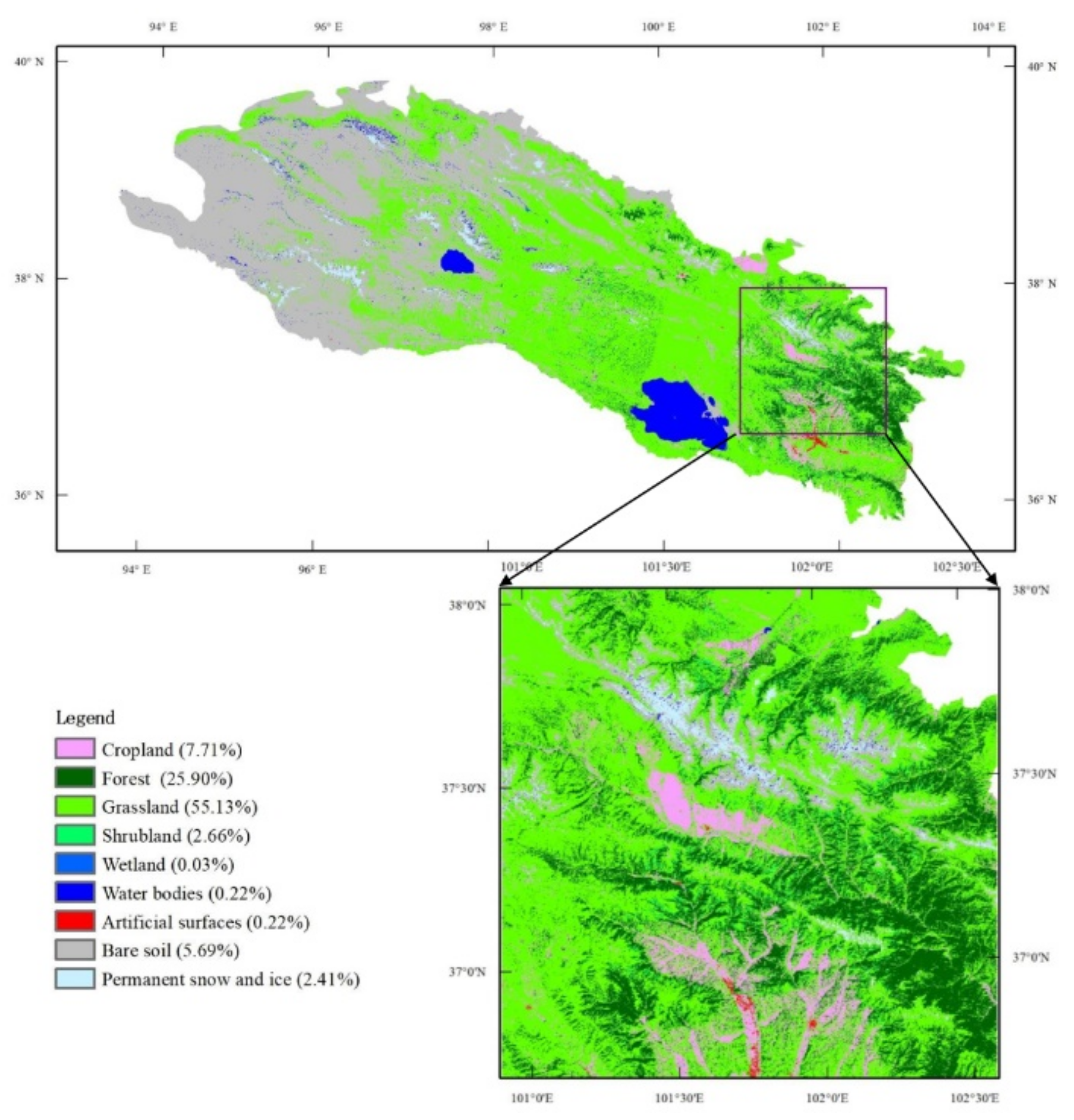
The land cover in the Qilian Mountain range exhibits an obvious varying trend from northwest to southeast, as shown in Figure 1. The land cover majorly consists of grasslands and bare soils in this region. The northwest part of the study region is poorly vegetated and is mainly covered by deserts and some oases. The middle region is mainly dominated by grasslands with minimal wetlands. The vegetation in the southeastern region is more diverse and fragmented and consists of grasslands, forests, croplands, shrublands, and some unvegetated land cover types. The vegetation in the Qilian Mountain range commonly presents a single growing season from May to September, and the growing season length is mainly influenced by climatic variables, including precipitation and temperature [34,35,36]. A heterogeneous region in the southeastern part (red square in Figure 1) is chosen for a deep study and analysis.

Figure 1.
Land cover map of the Qilian Mountain range region and study area: the proportions of each land cover type in the study area are shown in the legend.
2.2. Surface Reflectance Product
The Landsat mission, first launched in 1972, offered continuous high-resolution remote sensing records for over 30 years [7]. The released level-1 surface reflectance (L1TP) data from Landsat 5 Thematic Mapper (TM), Landsat 7 Enhanced Thematic Mapper(ETM+), and Landsat 8 Operational Land Imager (OLI) were used to calculate the NDVI values in this paper. The L1TP surface reflectance data are radiometrically calibrated and orthorectified using ground control points (GCPs) and digital elevation model (DEM) data to correct for relief displacement, which make the data suitable for pixel-level time series analysis. Atmospheric correction was processed by the Landsat Ecosystem Disturbance Adaptive Processing System (LEDAPS) and the Land Surface Reflectance Code (LaSRC) for the TM/ETM+ and OLI data, respectively. The products also provide a quality assessment (QA) band to identify clouds and cloud shadows using the CFMask algorithm [37]. For the Qilian Mountain range region, the available L1TP products started from 1986. The Landsat images are provided with the WGS-84 coordinate system with the projection of Universal Transverse Mercator (UTM). Due to sensor faults, striped gaps exist in some of the Landsat-7 images. Some values along the edge of Landsat 5 images are abnormal; there are values masked by an erosion procedure in this paper.
Level-1C reflectance data of the study region collected on the 193rd day of 2017 from the Sentinel-2A multispectral instrument (MSI) was acquired for validation (Section 4.4). Atmospheric correction was performed using Sen2Cor software provided by the European Space Agency (http://step.esa.int/main/thirdparty-plugins-2/sen2cor/). The cloud percentage data were acquired from the QA bands. Pixels in which the cloud percentage was over 70% were masked in the validation. The Sentinel-2 images have a spatial resolution of 10 m and are averagely aggregated to a resolution of 30 m for the evaluation.
2.3. Land Cover Dataset
The land cover product of the Qilian Mountain range region, providing 30 m resolution land cover maps for every five years from 1985 to 2017, was used to identify vegetation types in this study [38]. In this product, the time series data of 2015 were first constructed by using Landsat-8/OLI data, the knowledge of different land cover features was summarized according to the different NDVI time series curves presented by various temporal features, the extraction rules for different feature information were set, and the land cover classification map of 2015 was finally obtained [39,40]. The land surface was classified into 10 types: cropland, forest, grassland, shrubland, wetland, water bodies, artificial surfaces, bare soil, permanent ice, and snow. Based on the validation from field surveys and Google Earth images, the overall accuracy of the land cover map from 2015 was 92.19%. Then, samples of each land cover type were selected based on the 2015 land cover map. A random forest classifier using the reflectance information and vegetation indices, including NDVI, MNDWI (modified normalized difference water index), and NDBI (normalized difference built-up index), was constructed in the Google Earth Engine platform and used to generate the landcover maps every 5 years from 1985 to 2017. By comparing the two sets of classification products in 2015, the land cover products obtained based on the Google Earth Engine platform have good consistency with the classification products obtained based on the time series method. To indicate the vegetation type of each year, the land cover map of the nearest year was used. The MODIS 500-m Land cover dataset (MCD12Q1) with the IGBP classification scheme was used to distinguish between evergreen forests and deciduous forests.
2.4. ERA-5 Climate Reanalysis Dataset
ERA-5 [41] is the fifth-generation global atmospheric reanalysis dataset produced by the European Center for Medium-Range Weather Forecast (ECMWF, https://cds.climate.copernicus.eu/cdsapp#!/home). It provides climate variables with higher spatial and temporal resolution than those provided by the ERA5-interim product [42]. All ERA-5 atmospheric variables were interpolated at a 0.25° × 0.25° spatial resolution using a bilinear method from the native grid (0.5° × 0.5°). Three climate variables, at a daily resolution, were used in this study: the 2-m surface temperature (TEM), surface solar radiation downwards (SSRD), and total precipitation (PRE). The 2-m surface temperature was calculated by interpolating between the lowest model level and the Earth’s surface, taking into account the atmospheric conditions. The SSRD is the amount of solar radiation (also known as shortwave radiation) reaching the surface of the Earth. This variable comprises both direct and diffuse solar radiation. The PRE refers to the accumulated liquid and frozen water, including rain and snow, that falls to the Earth’s surface. Previous studies suggest that the use of ERA-5 is appropriate in the study region [42,43].
3. Method
Vegetation growth is constrained by climate factors and is sensitive to climate change [44,45]. When the vegetation types are unchanged, interannual variations in vegetation growth are mainly controlled by changes in climatic factors. In the study region, the dominate controlling factor was precipitation followed by temperature according to previous studies [34,35,36]. The response of vegetation to climate change is dependent on the vegetation type. Here, we focused on depicting changes in the NDVI time series given observed changes in the climate variables in adjacent years.
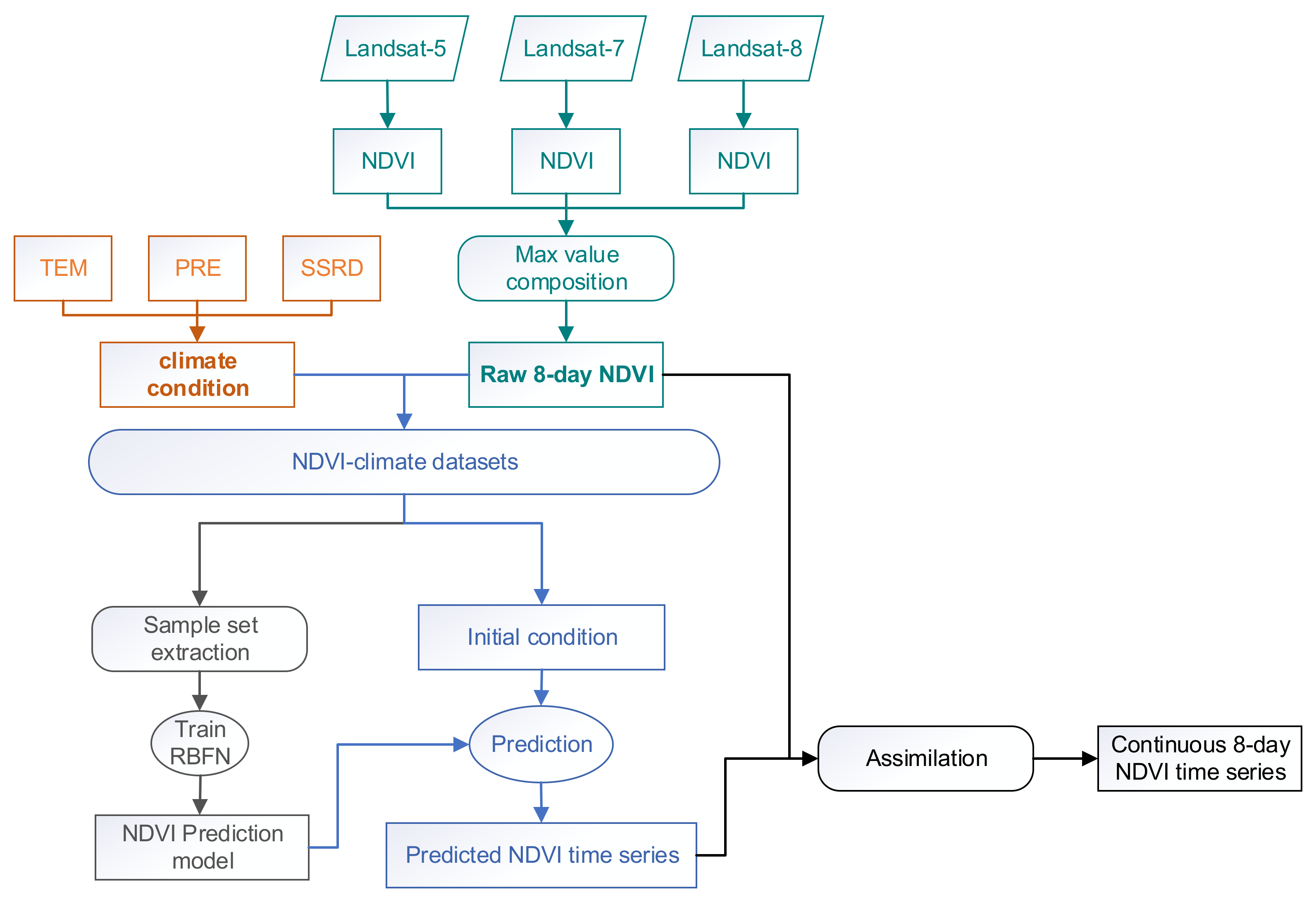
The objective of this study was to generate long-term continuous NDVI time series with available Landsat images. As shown in Figure 2, the method is composed of 4 parts: (1) the composition of raw NDVI time series and corresponding climate variables, (2) the construction of a prediction model for NDVI time series, (3) the prediction of NDVI time series, and (4) the adjustment of the predicted data to fit the observed NDVI values.
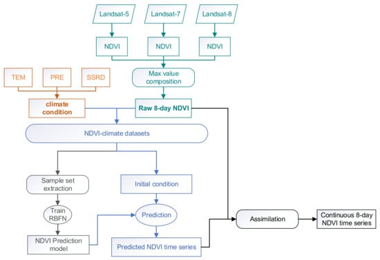
Figure 2.
Conceptual framework of the reconstruction of the Landsat Normalized Difference Vegetation Index (NDVI) time series.
3.1. Generation of Raw NDVI Time Series and Corresponding Climate Variables
The NDVI is first calculated from all available Landsat SR products in the study area. NDVI is calculated as follows:
where is the surface reflectance in the red band and is the surface reflectance in the near-infrared band. Clouds and cloud shadows identified by the QA information in the SR products were masked in the calculation, and an inward erosion procedure along the edges (≈8 pixels) was applied to the Landsat-5 images to handle abnormal values. To account for the spectral inconsistency that exists between the TM/ETM+ and OLI sensors, a linear transformation (Equation (2)) was made to the NDVI values of Landsat 5 and Landsat 7, according to a previous study [46], and the coefficients were derived using ordinary least squares (OLS) regression with a total of 6317 Landsat-7 ETM+ and Landsat-8 OLI images acquired over three summer and three winter months.
Then, each NDVI image was resampled to an identical projection and spatial reference (UTM 47N in the WGS-84 coordinate system in this paper) using bilinear interpolation for the following procedures. Finally, the NDVI images were mosaicked and composited for every 8-day period, yielding 46 NDVI maps in a given year. The maximum value composition method (i.e., the maximum value in the compositing period was chosen as the NDVI in an 8-day period) [47] was adopted here to reduce the influences of residual clouds or snow cover. The seasonal climate variables (i.e., total precipitation, mean temperature, and mean downwards solar radiation) corresponding to each pixel were calculated from the ERA-5 reanalysis dataset with the same geolocation (longitudes and latitudes). Different percentages and lengths of gaps were present in the composited Landsat NDVI datasets. The pixels with sufficient high-quality observations could be well reconstructed by traditional methods (e.g., HANTS and SG filter) [8,23].
3.2. Climate Integrated Gap-Filling (CGF) Method
We note that the gaps were more pronounced in older years due to the sparse observations obtained in these years. Traditional methods face challenges when reconstructing time series with large gaps. The key factor in the proposed method is the extraction of the information provided by pixels with sufficient high-quality observations and the reconstruction of those pixels with large gaps in the time series.
3.2.1. Link the NDVI Time Series of Adjacent Years with Radial Basis Function Networks (RBFNs)
An RBFN is used here to construct the relationship between the interannual change in the NDVI time series and climate variability. RBFNs, first proposed in 1988, are a kind of artificial neural network that uses radial basis functions as activation functions [48]; RBFNs have been considered the best network for function mapping and have been successfully applied in function approximations, time series predictions, and classification tasks [49]. As shown in Figure 3, we used the NDVI time series in year TS-1 and the difference in climate variables between two adjacent years to predict the NDVI time series in year TS-2. We assumed that the difference in climate variables (climate variability) drives the interannual changes of NDVI time series. Each climate variable was aggregated to a seasonal resolution (i.e., 4 values in a year) to indicate the climate variability of corresponding pixels (discussions on the temporal resolutions of the climate variables can be found in Section 5.1). Compared with NDVI data, climate data are much coarser in terms of spatial resolution, which means that several pixels share identical climate variability. In this case, the difference of the pixels is reflected on the difference in its NDVI time series. As many studies suggest, there exists a time lag (up to months) of the NDVI’s responses to climate variables. Therefore, we perform the NDVI prediction by RBFN on a yearly basis. The time-lag effects are expected to be learned by the RBFN model inherently. The RBFN model predicts NDVI time series for a given pixel in a target year, and these predictions are used as background NDVI time series for the following procedures. The prediction accuracy determines the precision of the gap-filling method.

Figure 3.
The structure of radial basis function networks (RBFNs) and the input and output nodes.
An RBFN is typically composed of 3 layers (as Figure 3 shows): an input layer, a hidden layer with an RBF activation function, and a linear output layer. In this study, the input vectors (x) are composed of 58 nodes: the NDVI time series in year-1 (46 nodes) and the differences in TEM, PRE, and SSRD between year TS-1 and year TS-2 (4 nodes of each climate variable). The output variables are the NDVI time series in year TS-2 (46 nodes).
Hidden nodes (), which have the same structure as the input vector x, were chosen from the training set. The RBF activation functions in each hidden node quantifying the “distance” between an input vector x and the center are formulated as follows:
where controls the radius of the function.
Then, the output of the network (i.e., the predicted NDVI time series) can be expressed as a weighted sum of hidden nodes, as follows:
where N is the number of hidden nodes and is the weight linking the hidden layer and the output layer.
The center vector , weight , and are determined in the training process. The first step is to select proper centers from the training set. The number of centers and the value of are usually determined by cross-validation. The second step is to calculate the weights to minimize the objective function:
where is the true time series in the training set.
The training of the RBFN was performed for every vegetation type separately. The number of nodes in the hidden layer and the parameter of the RBF need to be chosen carefully [50]. The inclusion of many hidden nodes allows for the acquisition of more accurate results but also takes more time due to the increased network size. The parameter controls the distance between the input and centers. A large means that the output would be closer to a specific center in the hidden layer, and a small would lead the output being close to the average of some centers in the hidden layer. In this paper, the number of hidden nodes and are set to 500 and 0.5, respectively, after a cross validation under different parameter combinations.
K-means clustering is applied to the training set, and the clustering centers are used as hidden nodes in the RBFN. PCA (principle component analysis) is used to reduce the processing time of the K-means clustering.
The training of the RBFN could be expressed in a matrix form as follows:
where M is the size of the training set, are the outputs of the hidden nodes, and we can acquire the weights through the ordinary least square method below.
3.2.2. Generation of the Sample Set for the RBFN Model
The sample set is collected for each vegetation type from the NDVI-climate dataset generated in Section 3.1 and is used for training and testing of the RBFN model. Two aspects are considered in the extraction of the sample set: (1) the samples are distributed as evenly as possible in time and space to account for different patterns in the study region. (2) The NDVI time series in the samples are less affected by gaps, and the NDVI trajectory can be reconstructed correctly by traditional methods.
The sample set was extracted from every set of two adjacent years. The study region (5000 × 5000 pixels) was evenly split into several blocks (100 × 100 pixels) in space, and the sample set extraction was performed in each block and each vegetation type separately. Two criteria were used in this extraction: (1) quality threshold (which ensures that the NDVI trajectories can be correctly reconstructed), where the overall gap percentages (GP) for the two years are below 50% (<23), and the max continuous gap lengths (GL) are less than 32 days (<4), and (2) statistical threshold (which ensures that samples with the best observation quality are extracted), where the lowest 10th percentile of the GP and GL of each block are used. Then, the minimum of the quality and statistical thresholds are set as the final selection thresholds:
Hence, the extraction of the training set is performed with the following procedures. (1) Calculate the gap percentage and maximum continuous gap length of each pixel in adjacent years. (2) Evenly divide the region into several blocks (100 × 100 pixels). (3) Calculate the lowest 10th percentile of the gap fraction and the length of maximum continuous gaps () over each block. (4) Pixels that meet the selection criterion, i.e., and GL , are extracted to the sample set. Finally, HANTS is applied to the extracted samples to obtain a gap-free NDVI time series. Table 1 shows the size of the sample set of each vegetation type. For each vegetation type, 75% of the sample set is used for training and the other 25% is used for testing.

Table 1.
Size of the sample set of each vegetation types.
3.2.3. Prediction and Postprocessing
We chose to fill the gaps backwards in time as the data quality is better in more recent years. Thus, the NDVI time series in the target year is predicted by the trained RBFN model with the NDVI time series of its following year and the corresponding climate variability data. A seamless NDVI time series in the study region is needed to start the prediction. The average of the year from 2014 to 2018 is calculated and serves as the initial condition. Then, the predictions are recursively performed starting from 2018 to 1986. The predicted NDVI time series can deviate from real observed data due to the accuracy of the RBFN model. Thus, an adjustment (postprocessing) to the predicted time series is needed to match the observed data. Over each year, the raw NDVI observations are used to adjust the amplitude of the predicted NDVI time series in a piecewise way. Referring to CACAO [17], the adjustment procedures are as follows. (1) Split the predicted time series into several parts with local extreme points. Each part is extended by 2 points to ensure the integrity of the adjusted results. (2) For each part, a scale coefficient, k, is calculated to minimize the bias between the adjusted NDVI and observed NDVI values, as follows:
where is the predicted NDVI time series from the RBFN model and is the final reconstructed NDVI time series after the adjustment. The term provides the scale coefficient for each NDVI value in the time series. We can calculate the coefficient k for each part by applying least square regression to available observed NDVI, as follows:
where is the ith observed reference NDVI value in the time series and is the corresponding predicted NDVI.
NDVI values below 0.1 are deemed snow contamination, which is masked in the adjustment. Unreasonable adjusted results are rejected (e.g., reconstructed NDVI values exceed 1, and mean bias values between the reconstructed and observed values are larger than 0.1 except for in the evergreen forest).
3.3. Evaluation Approach
3.3.1. Comparison with Other Time Series Reconstruction Methods
Three widely used time series reconstruction methods (HANTS, SG filter, and climatology) were implemented for the comparison and evaluation in this study. The HANTS method uses the sum of harmonics to fit the observed NDVI time series. The number of harmonics was set to 4, as suggested in [51]. The SG filter uses polynomials to fit the upper envelope of a NDVI time series in moving windows. The polynomial order and window width were set to 4 and 13, respectively, as suggested in a previous paper [9]. Climatology (averaged over multiple years) is also implemented in the comparison of long time series reconstructions (Section 4.4.2).
The evaluation in this study focused on gap-filling performance. The performances of the methods were evaluated using NDVI time series with simulated gaps and real gaps. Two kinds of gaps were considered: random gaps (with different gap percentages) and continuous gaps (with different gap lengths). For the simulated gaps, a portion of the time series in the sample set was extracted as a reference NDVI time series and then added with various simulated gaps to evaluate the gap-filling performance. For real gaps, the performance was evaluated in the image extent using Sentinel-2 images (introduced in Section 2.2) as a reference and in the long time series using real observation data as a reference separately.
3.3.2. Evaluation Metrics
The root mean squared error (RMSE) and mean absolute error (MAE) quantify the accuracy of reconstructed NDVI values:
where and are the reconstructed and reference NDVI values for date t and pixel j, is the number of points in a time series (46 for an 8-day time series in this paper), and N is the total number of pixels in an image.
Different reconstruction methods may fail under different circumstances. We used the reconstruction index (RI) to express the ratio of the number of pixels successfully reconstructed to the number of total processed pixels. The reconstructed values that are not within a reasonable range (−0.2–1 in this study) are deemed failed pixels. The RI is calculated as follows:
where and represent the number of successfully reconstructed pixels and the total number of processed pixels, respectively.
4. Results
4.1. Theoretical Performance of RBFN-Based NDVI Prediction Model
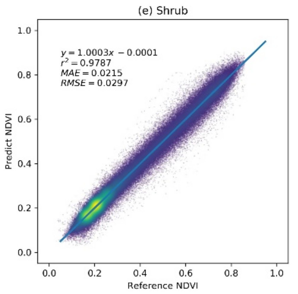
The prediction accuracy of the RBFN model was evaluated using the extracted sample set. Figure 4 shows the scatter plot between the predicted NDVI values and the reference NDVI values for different vegetation types. The results indicate that the RBFN model achieved a high prediction accuracy for different vegetation types in the study region. The regression lines of each vegetation type are close to the 1:1 line and have r2 values over 0.95, indicating that the predicted NDVI values are well correlated with the true NDVI. For the grass, shrub, and deciduous forest vegetation types, the RBFN has a better prediction performance with MAE and RMSE values of approximately 0.023 and 0.03, respectively. In addition, the dispersion does not change much with an increasing NDVI value. The MAE and RMSE of the crop and evergreen forest vegetation types, for which the growth processes are less constrained by the climate variables, are slightly higher (approximately 0.03 and 0.04, respectively). The results demonstrate that the RBFN model can accurately predict the NDVI time series for different vegetation types.


Figure 4.
The accuracy of the radial basis function network (RBFN)-based NDVI prediction model over different vegetation types: a brighter color (yellow) denotes a higher point density, and a darker color (deep blue) denotes a lower point density.
4.2. The Gap Patterns of Raw Composited Landsat NDVI Maps
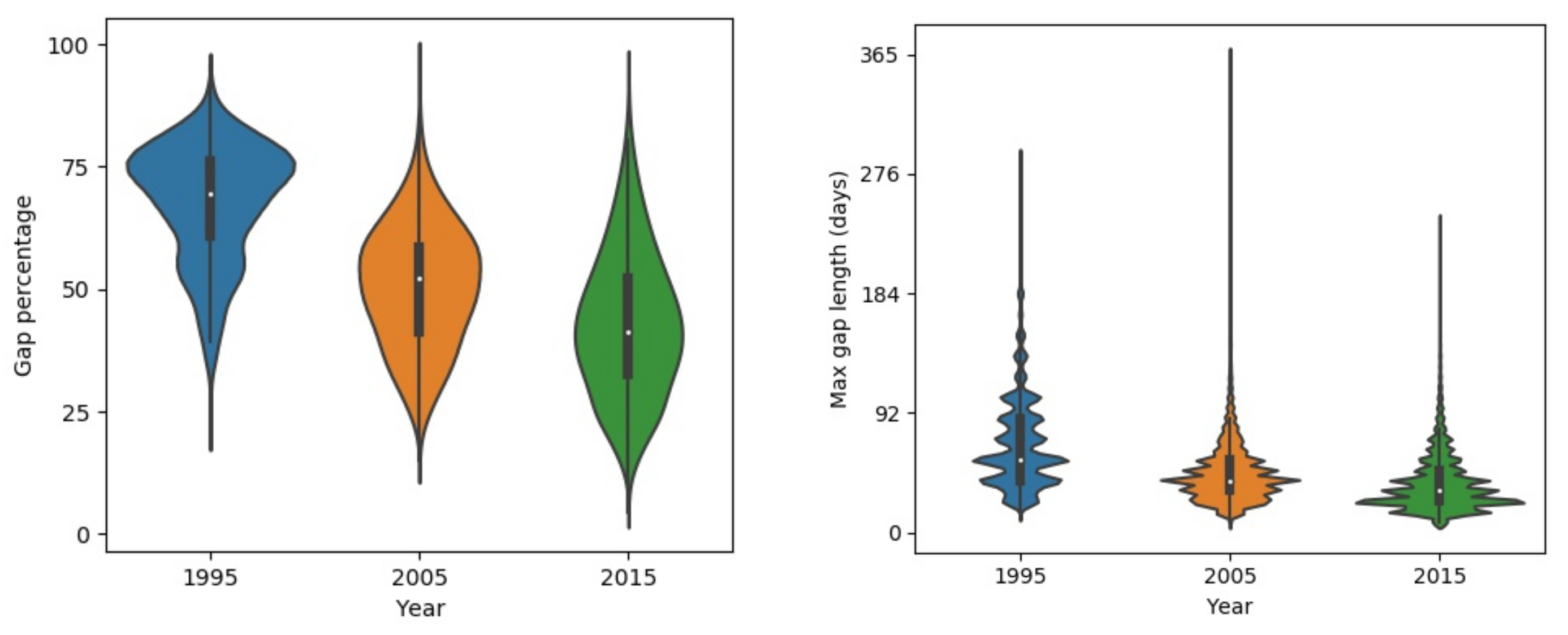
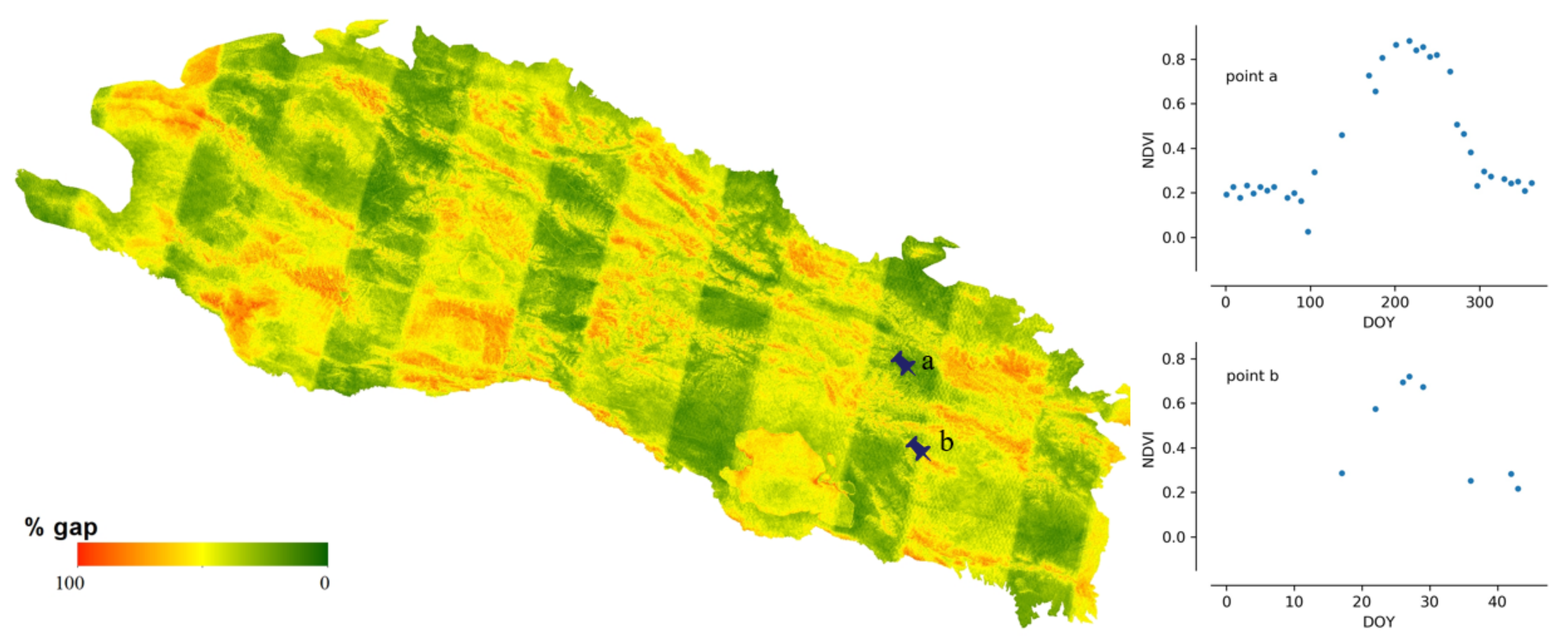
The gaps in the raw composited NDVI map result from multiple factors. Figure 5 shows the distributions of gap percentage and maximum continuous gap lengths in the Qilian Mountain range region in 1995, 2005, and 2015. There exists evident differences in the gap patterns among the 3 years because the number of Landsat satellites in orbit was different in different years. There was only one satellite (Landsat-5) before the 2000s and two satellites (Landsat-7 and Landsat-8) after the 2000s. The gap percentage decreased with years in the study area. The average gap percentages were around 70%, 55%, and 40% in 1995, 2005, and 2015, respectively. The gap percentages of 2005 and 2015 approximate normal distributions. The distribution was skewed to a high gap percentage in 1995, which indicates that large gaps existed in the data. The maximum continuous gap lengths exhibited similar patterns to those of the gap percentages. The peak value in the distribution decreases as the year increases. The peak values of max continuous gap lengths were approximately 64, 48, and 32 days for 1995, 2005, and 2015, respectively. Figure 6 shows the gap percentage map of the Qilian Mountain range region in 2015. It presents a banded contexture of high (over 50%) and low (below 50%) gap percentages. The bands of low gap fractions are formed because they are located in the overlapping parts of adjacent Landsat image footprints. Mountainous areas commonly have higher gap fractions, as those regions are more easily affected by clouds and snows. Figure 6 displays the raw NDVI time series at two points. It is shown that the phenological trajectory of point a can be correctly depicted by the observed NDVI. However, the observed data at point b are too sparse to represent its phenological trajectory. Thus, it is possible to use effective information from pixels with small gaps to reconstruct pixels with large gaps.

Figure 5.
Gap patterns of raw Landsat NDVI time series in 1995, 2005, and 2015 separately.

Figure 6.
The fraction of gaps in composited Landsat 8-day NDVI time series from 2015 in the Qilian Mountain range region.
4.3. Quantitative Evaluation of Different Methods with Simulated Gaps
The performances of the different methods (HANTS, SG filter, and CGF) were evaluated using the NDVI time series with different gap percentages and different continuous gap lengths added. First, gaps with different percentages were randomly added to the NDVI time series. Then, the three methods were applied to generate the reconstructed NDVI time series. The MAE and RMSE values were calculated with the reconstructed values and reference values in gaps. As Figure 7 shows, the three methods showed similar performances (MAE of approximately 0.035 and RMSE of approximately 0.042) when the gap fraction was below 50%. The HANTS method performed slightly better than the other methods when the gap percentage was small (<40%). As the gap fraction increased, the accuracy of the HANTS and SG filter methods displayed an obvious declining trend. When the gap fraction reached 80%, the traditional methods induced considerable biases while the CGF method still worked with satisfying accuracy (MAE below 0.04 and RMSE below 0.08). Then, continuous gaps were added, starting from the growing season, with different lengths (10% to 50% of the whole time series). As shown in Figure 8, the methods performed similarly when the gap length was small (10%). As the gap length increased, the biases of the HANTS and SG filter methods increased rapidly. Large uncertainties in the reconstructed time series were introduced with traditional methods when continuous gaps (over 30%) existed during the growing season. The only stable method was the proposed CGF method, which had a largest MAE of 0.05 and RMSE of 0.075 when the gap lengths reached 50% of the total time series. Thus, the CGF method is suitable for the reconstruction of Landsat NDVI, which is usually contaminated with obvious gaps (as shown in Figure 5).

Figure 7.
The performance of the NDVI reconstruction model with different gap fractions (gap%).

Figure 8.
The performance of the NDVI reconstruction model with different consecutive gap lengths.
4.4. Quantitative Evaluation of Different Methods with Landsat Data
4.4.1. Comparison with Other Time Series Reconstruction Methods
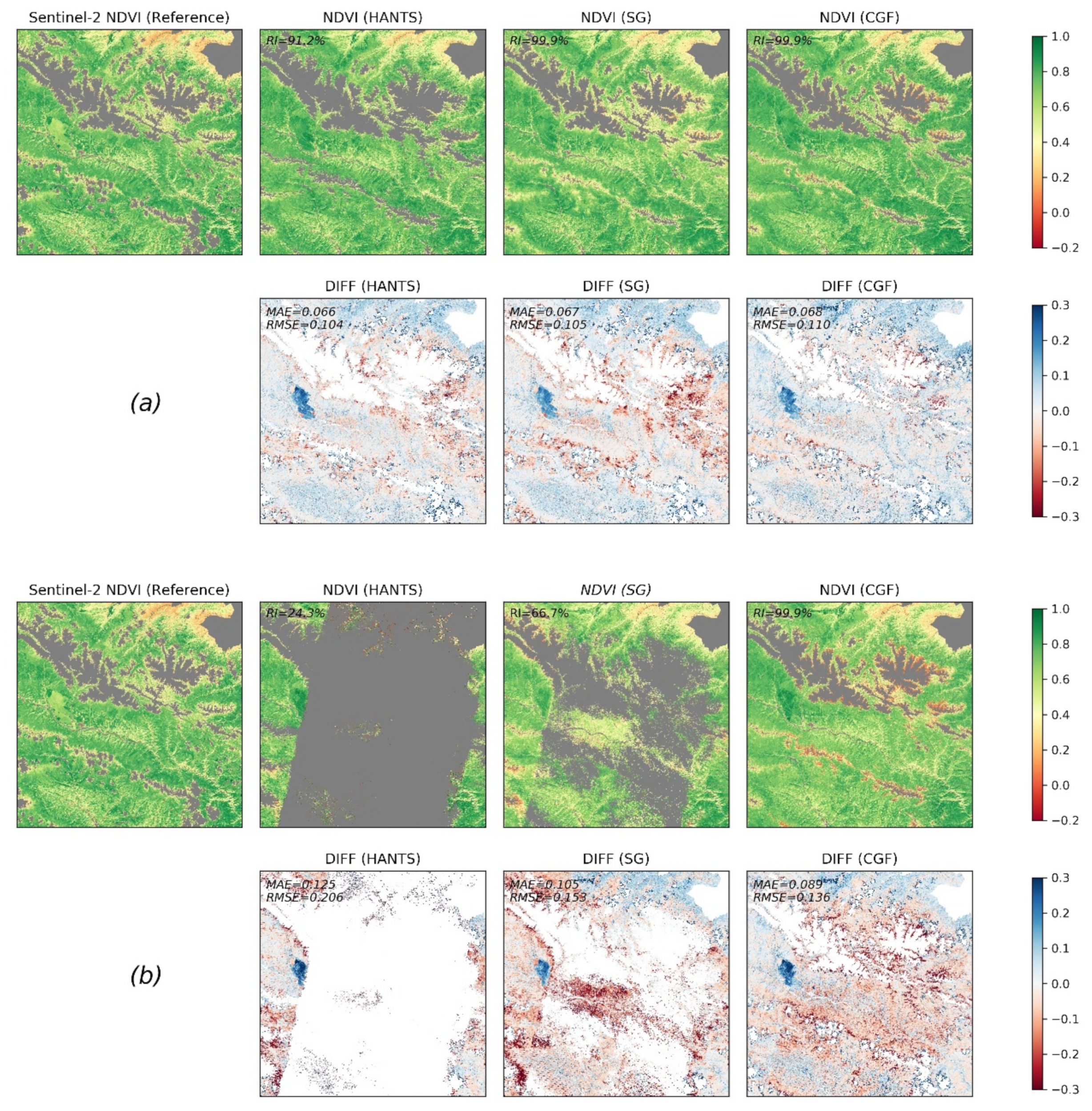
We evaluated the performance of different methods in reconstructing Landsat NDVI maps with contrasting gap patterns. Two kinds of gap patterns were considered: the real gap patterns in 2017 (average gap percentage of 52.5%) and the gaps patterns in 1997 (average gap percentage of 69.2%). The NDVI maps in 2017 were firstly reconstructed with the real gaps in 2017 (Figure 9a). Then, the pixels corresponding to gaps of 1997 were removed. We reconstructed the new NDVI maps with the gap patterns in 1997 finally (Figure 9b). Figure 9 shows a comparison between the reconstructed NDVI maps and raw NDVI maps for DOY (day of year) 193 in 2017 under different gap conditions. The Sentinel-2 NDVI map on that day was used as a reference. The non-vegetated area and the clouds and shadows in the Sentinel-2 map are masked and are displayed in grey in Figure 9. For the real gap patterns in 2017, the methods all performed well in the time series reconstruction (MAE and RMSE of approximately 0.067 and 0.105, respectively). The reconstructed NDVI maps exhibited consistent spatial patterns when compared to the reference data. In general, the HANTS and SG filter methods performed slightly better than the CGF method when the gap percentage was not large. The RI of HANTS was relatively low (91.2%), and failures mainly occurred at the mountain edges. When applying reconstruction with the gap patterns of 1997, the RIs of the HANTS and SG filter methods significantly decreased, which means that a large proportion of pixels could not be processed by the two methods, e.g., the HANTS and SG filter methods only processed 24.3% and 66.7% of the total pixels in this region, respectively. Furthermore, the RMSEs of the HANTS and SG filter methods (0.206 and 0.153, respectively) are larger than the RMSE of the CGF method (0.136), even for the successfully reconstructed pixels. Thus, the CGF method is the only applicable method when dealing with the large gaps that widely exist in Landsat NDVI maps before the 2000s.
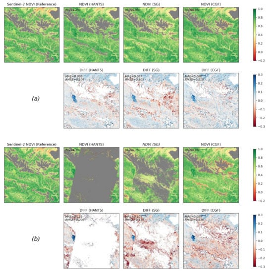
Figure 9.
Comparison of reconstruction methods with Landsat observation data from 2017. (a) Reconstruction results in DOY (day of year) 193 in 2017 with actual gap patterns. (b) Reconstruction results with gap patterns of Landsat composited NDVI in 1997.
4.4.2. Performance in Reconstructing Long-Term Landsat NDVI
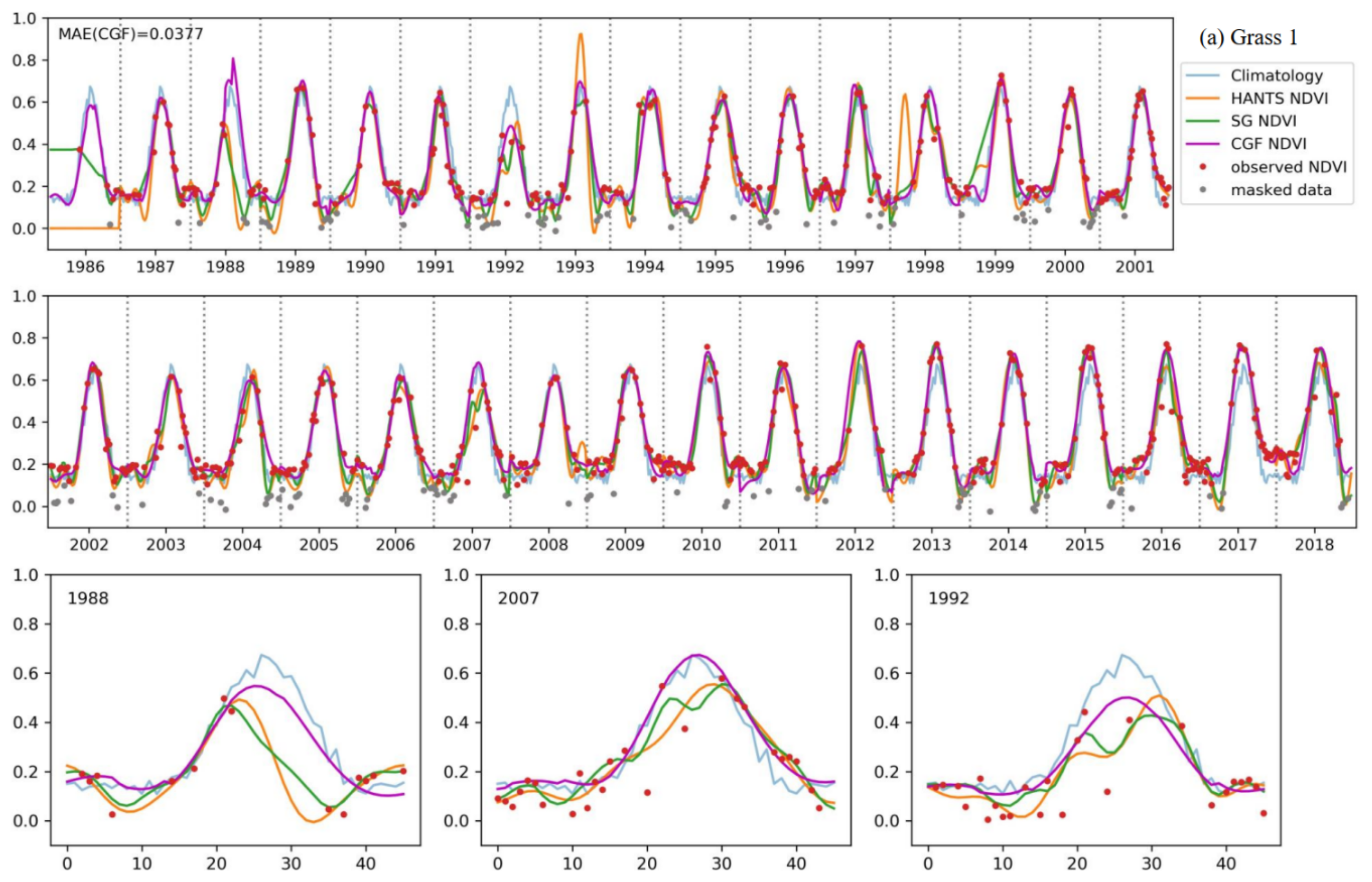
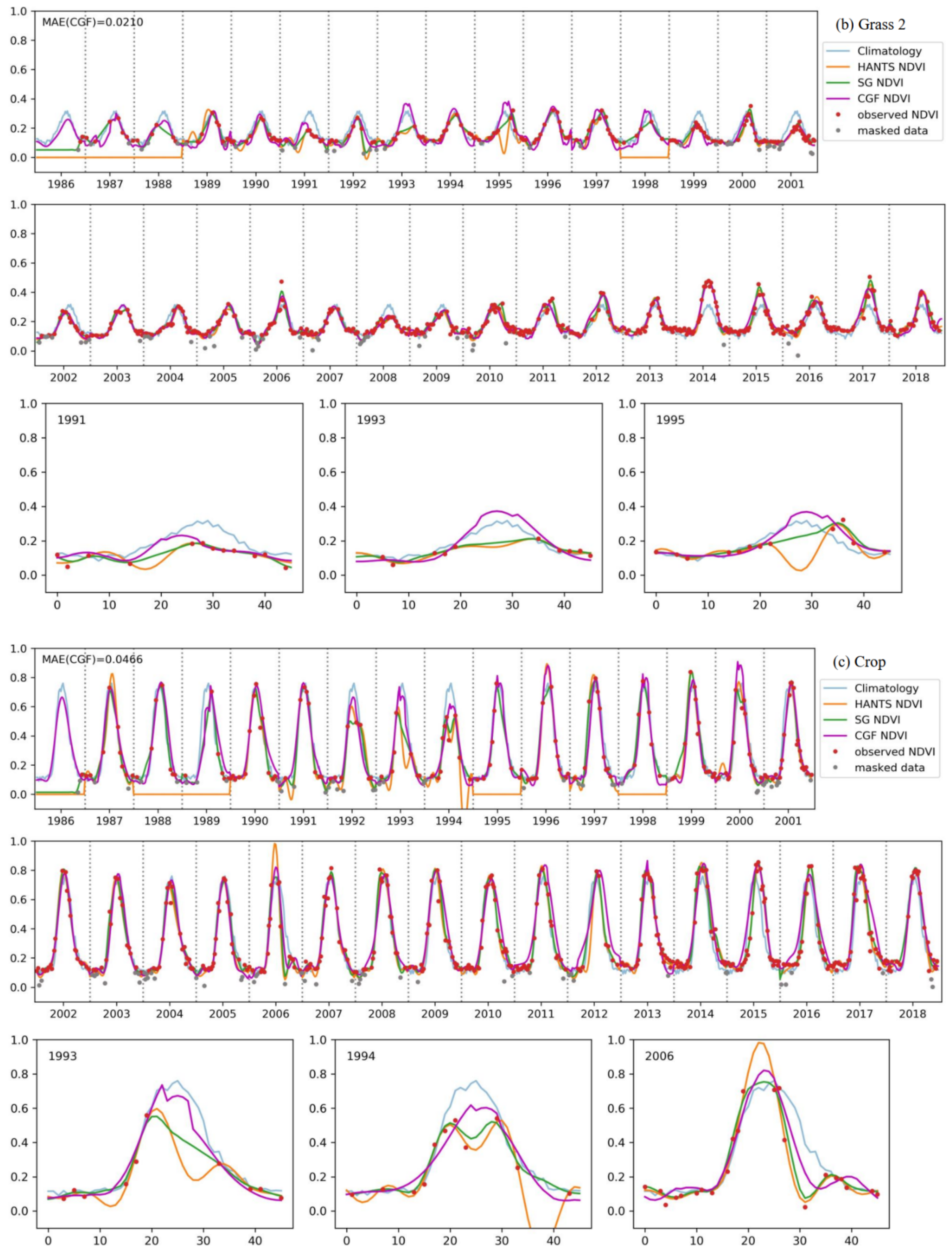
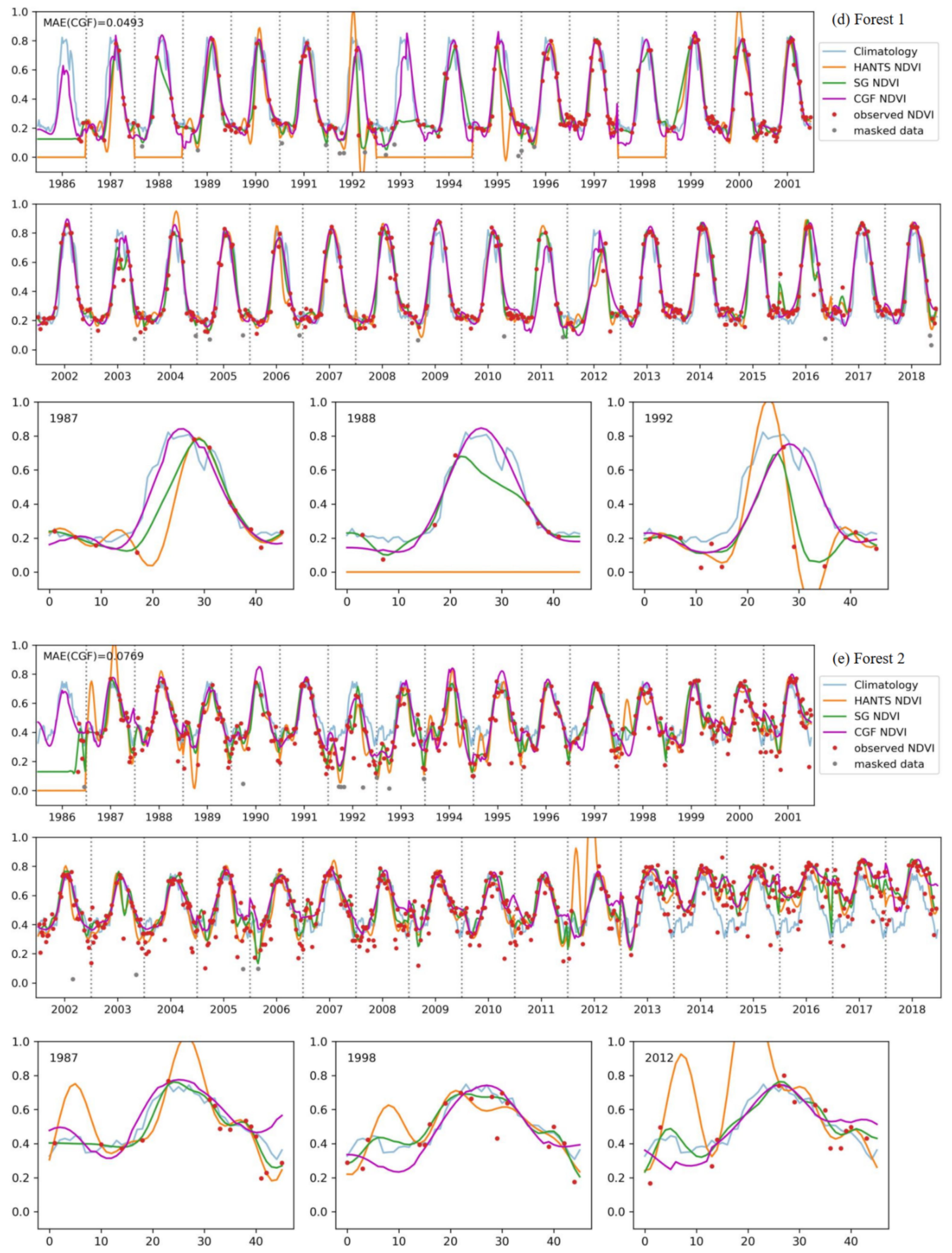
Figure 10 shows a comparison of the reconstruction methods for long NDVI time series of different vegetation types. The traditional reconstruction methods (HANTS and SG filter) performed well, as expected, when the observed data were sufficient (usually in the years after 2000). However, when the observed data were sparse in the time series, the traditional methods usually failed or yielded unreasonable results. The HANTS method failed when there were fewer than 7 observed data in a year and induced large errors when the observed data were sparse, e.g., in 1992 for forest-1 and in 1987 for forest-2. When key points were missing, the SG filter method introduced unrealistic phenology trajectories due to its linear interpolation procedure (e.g., in 1993, as shown in Figure 10c). The HANTS and SG filter methods are sensitive to undetected outliers when the available observation data are sparse, e.g., in 1992 and 2007 for grass-1. Gaps in the key growth periods lead to the traditional methods yielding false NDVI trajectories. A gap in the peak region induced the loss of reconstructed growing seasons in the reconstruction results of 1991, 1993, and 1995 for grass-1. The gaps in the growing period in 1987 for forest-1 and during the senescence period in 1988 for grass-1 led to unreasonable HANTS and SG results. Thus, the traditional methods cannot correctly reconstruct the NDVI time series when large gaps exist in the NDVI time series. The climatology method can produce NDVI time series given large gaps. However, the results neglected annual changes in vegetation growth, which is not in accordance with the actual situation (e.g., the year after 2013 for forest-2). The climatology method could yield unreasonable results when the vegetation type changes over the years (for example, if grasslands transferred to bare soils or croplands). Comparably, the performance of the CGF method was more stable under different circumstances. With the incorporation of climate variables, the CGF method exploits the relationship between NDVI and climate variables that is generated from the data itself. The reconstruction MAE is generally approximate 0.05 (except for that of the evergreen forest), which demonstrates the effectiveness and accuracy of the proposed CGF method in the reconstruction of long-term Landsat NDVI time series.
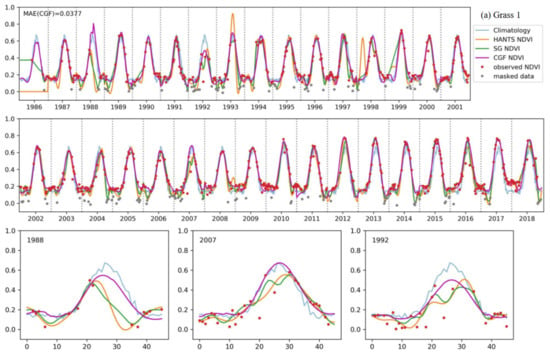

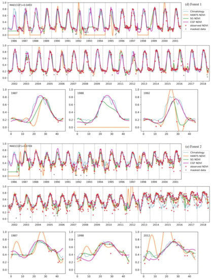
Figure 10.
The performance of the NDVI prediction model over different vegetation types ((a–e) represent different samples of different vegetation types) for long time series. Specific cases with significant difference in some years are highlighted for each vegetation type.
5. Discussion
5.1. The Role of Climate Data and Comparison with Existing Methods
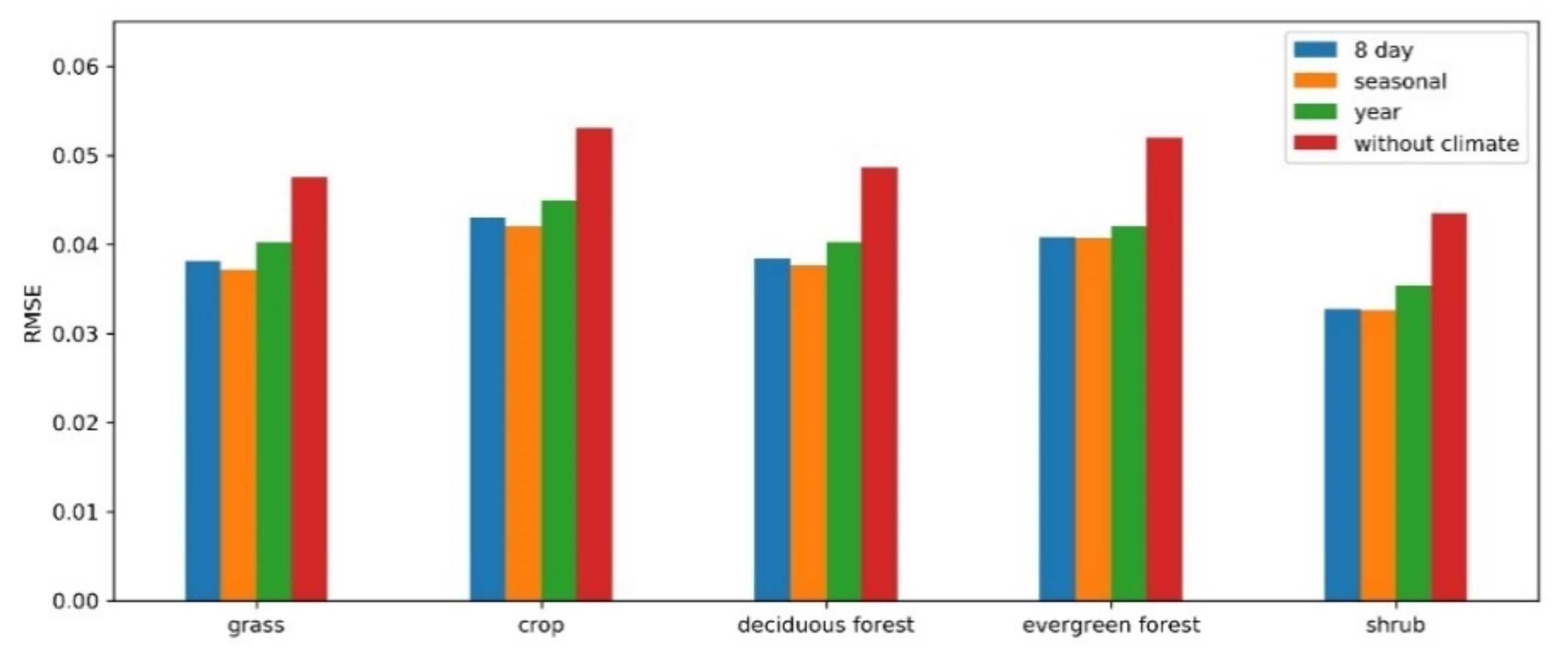
The vegetation growth in a specific region is constrained by its climatic conditions. In this study, the difference in climate variables between adjacent years is used as a conditional parameter that helps to find similar patterns more accurately for the target pixel. The role of climate data and the structure (compositing period) of the climate variables in the RBFN prediction model are studied for different vegetation types. Five thousand samples of each vegetation type were extracted from the sample set generated in Section 3.2.2. Then, the RMSE was calculated for the prediction results from the RBFN models using different climate data structures (i.e., without climate, 8-day, seasonal, and yearly). As Figure 11 shows, similar results were exhibited for all these vegetation types. The RBFN model predictions conducted without climate data, which resulted in higher RMSEs for all vegetation types, significantly decreased the prediction accuracy. Comparatively, the models in which the seasonal climate variables were incorporated achieved the best performance in different vegetation types. More generalized climate data (e.g., yearly) may not be sufficient to constrain vegetation changes, while a higher temporal frequency may be sensitive to bias in climate variables. Thus, climate data improve the prediction accuracy of RBFN models, and a seasonal structure is most effective in this task.

Figure 11.
The influence of climate data in the RBFN model for different vegetation types.
We compared the proposed CGF method with existing time series reconstruction methods, including HANTS and SG filter, which only exploited the observation data in the current year. For a pixel with sufficient observation data, the traditional methods could generate high-quality continuous time series with lower risks. The CGF method also used HANTS to reconstruct the time series in the extracted sample set to ensure quality. For the raw Landsat NDVI maps, large gaps could not be neglected and directly reconstructed by traditional methods, especially in the years before 2000. The major role of the CGF method was using prior information generated from pixels with sufficient high-quality observations to reconstruct the pixel presented with large gaps in the time series. The CACAO approach was also designed to generate long time series records from AVHRR data, using observations to adjust unified phenology trajectories [17]. However, the phenological shifting parameter could not be correctly determined using Landsat data in which large gaps were presented in the time series. Phenology variations were accounted for by the RBFN model developed in this study. Land cover changes could be evident at Landsat’s 30 m resolution, which conflicts with its assumption. The STSG method was developed to resolve the continuous gaps in the MODIS NDVI time series data. However, the low temporal frequency of high-resolution satellites limits the application of this method for Landsat data [20]. Climatology neglects interannual variations in NDVI time series. Land cover transitions also induce large errors in climatology. The CGF method provides a proper approach to reconstructing long-term Landsat NDVI time series.
5.2. Uncertainties and Limitation in the CGF Method
Some uncertainties should be noted in the CGF method. The major component of the CGF method involves using the RBFN model to predict the phenological trajectories of the target year. Machine learning techniques (e.g., artificial neural networks) have been proven to be efficient in predicting vegetation conditions as well as drought events [52]. RBFN used in this paper searches similar patterns in the training set to generate the predicted NDVI time series. Vuolo et al. [53] also used templates (time series of pixels characterized by a high number of valid observations in the temporal dimension) to fill the gaps in the time series of Landsat reflectance data. RBFN converts the search procedure of similar templates to a forward networking structure and significantly decreases the computational intensity in reconstruction. The climate data used in this paper also increase the searching accuracy. Several factors could influence the prediction accuracy of the RBFN model. First, due to the representativeness of the extracted training set, the training set should ideally contain all different patterns of the specific vegetation types to ensure the fidelity of the prediction results in most cases. In this study, the samples were extracted evenly in space and time (Section 3.2.2) to ensure their representativeness of the study region. The results verified the effectiveness of the model. However, in some regions, e.g., tropical regions, sufficient and representative training sets cannot be generated due to frequent clouds and rains. The effectiveness of the CGF method in these regions needs further validation. Second, the centers in the RBFN model affect the prediction accuracy. A larger number of centers theoretically increases the prediction accuracy but also increases the processing time simultaneously. The parameters used in this study represent a tradeoff between accuracy and time complexity. The parameter values are related to the diversity of vegetation growth and the climatic conditions in the study region. Additionally, NDVI changes caused by anthropogenic activities and extreme events, e.g., natural disasters and forest fires, may not be captured in the RBFN model. The CGF method can only be used to fill gaps for vegetation with normal growth. As the RBFN model uses climate data to drive the prediction model, it is not encouraged to use the predicted NDVI in climate change studies.
The 30 m land cover maps released for every five years are used in this study. The inclusion of land cover types increased the prediction accuracy. Misclassifications in the land cover maps and transitions between years led to incorrect vegetation type specifications in some pixels. If the RBFN model yields incorrect results, postprocessing attempts to decrease the deviation as much as possible. When evident errors still exist in the final reconstructed time series, the consistency check detects these pixels and sets them as failures.
The CGF method uses the observed data to adjust the phenological trajectories predicted by the RBFN model. The predicted time series may present incorrect phenology patterns in some cases, indicating that similar patterns do not exist in the training set. When the difference is not significant, the adjustment could also generate acceptable results. However, when there are only a few observations, this adjustment could yield unrealistic values due to the uncertainty in the observation points. In this case, the results are rejected by the consistency check. Additionally, there is only a single growing season in this study region; thus, the performance of the CGF method in reconstructing a complicated time series (e.g., time series of multi-season crops) needs more experiments for validation. The experiments were performed in a region where vegetation growth is sensitive to the climate variables (precipitation and temperature). However, in regions where climate variables cannot constrain vegetation growth, the proposed CGF method may yield dissatisfactory results.
6. Conclusions
Gap filling is the most important issue in reconstructing NDVI time series from Landsat satellites. Due to the sparse revisit frequencies of high-resolution satellites, traditional reconstruction approaches face the challenge of dealing with large gaps in raw NDVI time series. In this paper, a climate-integrated gap-filling (CGF) method was proposed for the reconstruction of the historical Landsat NDVI time series. The CGF model considers the relationship of NDVI time series and climate conditions between two adjacent years. The differences in climate variables, including downward solar shortwave radiation, precipitation, and temperature, calculated from the ERA-5 climate reanalysis dataset were used to characterize the constrain factors of vegetation growth. Radial basis function networks were used to link the interannual NDVI time series with the differences in the climate variables, i.e., the RBFN yielded the predicted NDVI time series of year 1 given the NDVI time series of adjacent year 2 and the change in climate variables between the two years. Finally, the observed data from year 1 were used to adjust the predicted NDVI time series to obtain the final results. The experiments were performed in a heterogeneous region in the Qilian Mountains. The results demonstrated that the proposed method can be used to accurately reconstruct Landsat historical NDVI time series where vegetation growth is sensitive to the climatic conditions. The CGF method shows comparable accuracy in reconstructing time series with small gaps and outperforms existing time series reconstruction methods (e.g., HANTS, SG filter, and climatology) in Landsat NDVI time series contaminated by large gaps. The proposed method can also be used for other high-resolution satellites, e.g., the Sentinel-2 series and Chinese GaoFen-1/GaoFen-6 series.
Author Contributions
Conceptualization, W.Y., J.L., and Q.L.; methodology, W.Y.; validation, W.Y.; analysis, S.L.; data curation, X.Z. and Z.Z.; writing—original draft preparation, W.Y.; writ-ing—review and editing, W.Y., J.Z., Y.D., H.Z., X.Z., and J.L.; project administration, Q.L. All authors have read and agreed to the published version of the manuscript.
Funding
This research was supported by the National Key Research and Development Program (2018YFA0605503) and the National Natural Science Foundation of China (No. 41671374).
Conflicts of Interest
The authors declare no conflict of interest.
References
- Sellers, P.; Dickinson, R.; Randall, D.; Betts, A.; Hall, F.; Berry, J.; Collatz, G.; Denning, A.; Mooney, H.; Nobre, C. Modeling the exchanges of energy, water, and carbon between continents and the atmosphere. Science 1997, 275, 502–509. [Google Scholar] [CrossRef] [PubMed]
- Zhang, X.; Friedl, M.A.; Schaaf, C.B.; Strahler, A.H.; Hodges, J.C.; Gao, F.; Reed, B.C.; Huete, A. Monitoring vegetation phenology using MODIS. Remote Sens. Environ. 2003, 84, 471–475. [Google Scholar] [CrossRef]
- Tucker, C.J.; Pinzon, J.E.; Brown, M.E.; Slayback, D.A.; Pak, E.W.; Mahoney, R.; Vermote, E.F.; El Saleous, N. An extended AVHRR 8-km NDVI dataset compatible with MODIS and SPOT vegetation NDVI data. Int. J. Remote Sens. 2005, 26, 4485–4498. [Google Scholar] [CrossRef]
- Huete, A.; Didan, K.; Miura, T.; Rodriguez, E.P.; Gao, X.; Ferreira, L.G. Overview of the radiometric and biophysical performance of the MODIS vegetation indices. Remote Sens. Environ. 2002, 83, 195–213. [Google Scholar] [CrossRef]
- Maisongrande, P.; Duchemin, B.; Dedieu, G. VEGETATION/SPOT: An operational mission for the Earth monitoring; presentation of new standard products. Int. J. Remote Sens. 2004, 25, 9–14. [Google Scholar] [CrossRef]
- Fensholt, R.; Proud, S.R. Evaluation of earth observation based global long term vegetation trends—Comparing GIMMS and MODIS global NDVI time series. Remote Sens. Environ. 2012, 119, 131–147. [Google Scholar] [CrossRef]
- Woodcock, C.E.; Allen, R.; Anderson, M.; Belward, A.; Bindschadler, R.; Cohen, W.; Gao, F.; Goward, S.N.; Helder, D.; Helmer, E. Free access to Landsat imagery. Science 2008, 320, 1011. [Google Scholar] [CrossRef]
- Liu, R.; Shang, R.; Liu, Y.; Lu, X. Global evaluation of gap-filling approaches for seasonal NDVI with considering vegetation growth trajectory, protection of key point, noise resistance and curve stability. Remote Sens. Environ. 2017, 189, 164–179. [Google Scholar] [CrossRef]
- Chen, J.; Jönsson, P.; Tamura, M.; Gu, Z.; Matsushita, B.; Eklundh, L. A simple method for reconstructing a high-quality NDVI time-series data set based on the Savitzky–Golay filter. Remote Sens. Environ. 2004, 91, 332–344. [Google Scholar] [CrossRef]
- Chen, J.M.; Deng, F.; Chen, M. Locally adjusted cubic-spline capping for reconstructing seasonal trajectories of a satellite-derived surface parameter. IEEE Trans. Geosci. Remote Sens. 2006, 44, 2230–2238. [Google Scholar] [CrossRef]
- Jonsson, P.; Eklundh, L. Seasonality extraction by function fitting to time-series of satellite sensor data. IEEE Trans. Geosci. Remote Sens. 2002, 40, 1824–1832. [Google Scholar] [CrossRef]
- Beck, P.S.A.; Atzberger, C.; Høgda, K.A.; Johansen, B.; Skidmore, A.K. Improved monitoring of vegetation dynamics at very high latitudes: A new method using MODIS NDVI. Remote Sens. Environ. 2006, 100, 321–334. [Google Scholar] [CrossRef]
- Menenti, M.; Azzali, S.; Verhoef, W.; van Swol, R. Mapping agroecological zones and time lag in vegetation growth by means of Fourier analysis of time series of NDVI images. Adv. Space Res. 1993, 13, 233–237. [Google Scholar] [CrossRef]
- Verhoef, W. Application of harmonic analysis of NDVI time series (HANTS). In Fourier Analysis of Temporal NDVI in the Southern African and American Continents; Report 108; SC-DLO: Wageningen, The Netherlands, 1996; Volume 108, pp. 19–24. [Google Scholar]
- Atzberger, C.; Eilers, P.H. A time series for monitoring vegetation activity and phenology at 10-daily time steps covering large parts of South America. Int. J. Digit. Earth 2011, 4, 365–386. [Google Scholar] [CrossRef]
- Verger, A.; Baret, F.; Weiss, M. A multisensor fusion approach to improve LAI time series. Remote Sens. Environ. 2011, 115, 2460–2470. [Google Scholar] [CrossRef]
- Verger, A.; Baret, F.; Weiss, M.; Kandasamy, S.; Vermote, E. The CACAO method for smoothing, gap filling, and characterizing seasonal anomalies in satellite time series. IEEE Trans. Geosci. Remote Sens. 2013, 51, 1963–1972. [Google Scholar] [CrossRef]
- Gu, J.; Li, X.; Huang, C.; Okin, G.S. A simplified data assimilation method for reconstructing time-series MODIS NDVI data. Adv. Space Res. 2009, 44, 501–509. [Google Scholar] [CrossRef]
- Fang, H.; Liang, S.; Townshend, J.; Dickinson, R. Spatially and temporally continuous LAI data sets based on an integrated filtering method: Examples from North America. Remote Sens. Environ. 2008, 112, 75–93. [Google Scholar] [CrossRef]
- Cao, R.; Chen, Y.; Shen, M.; Chen, J.; Zhou, J.; Wang, C.; Yang, W. A simple method to improve the quality of NDVI time-series data by integrating spatiotemporal information with the Savitzky-Golay filter. Remote Sens. Environ. 2018, 217, 244–257. [Google Scholar] [CrossRef]
- Yuan, H.; Dai, Y.; Xiao, Z.; Ji, D.; Shangguan, W. Reprocessing the MODIS Leaf Area Index products for land surface and climate modelling. Remote Sens. Environ. 2011, 115, 1171–1187. [Google Scholar] [CrossRef]
- Julien, Y.; Sobrino, J.A. Comparison of cloud-reconstruction methods for time series of composite NDVI data. Remote Sens. Environ. 2010, 114, 618–625. [Google Scholar] [CrossRef]
- Kandasamy, S.; Baret, F.; Verger, A.; Neveux, P.; Weiss, M. A comparison of methods for smoothing and gap filling time series of remote sensing observations-application to MODIS LAI products. Biogeosciences 2013, 10, 4055–4071. [Google Scholar] [CrossRef]
- Robinson, N.; Allred, B.; Jones, M.; Moreno, A.; Kimball, J.; Naugle, D.; Erickson, T.; Richardson, A. A dynamic Landsat derived normalized difference vegetation index (NDVI) product for the conterminous United States. Remote Sens. 2017, 9, 863. [Google Scholar] [CrossRef]
- Zhu, X.; Helmer, E.H.; Gao, F.; Liu, D.; Chen, J.; Lefsky, M.A. A flexible spatiotemporal method for fusing satellite images with different resolutions. Remote Sens. Environ. 2016, 172, 165–177. [Google Scholar] [CrossRef]
- Liu, M.; Yang, W.; Zhu, X.; Chen, J.; Chen, X.; Yang, L.; Helmer, E.H. An Improved Flexible Spatiotemporal DAta Fusion (IFSDAF) method for producing high spatiotemporal resolution normalized difference vegetation index time series. Remote Sens. Environ. 2019, 227, 74–89. [Google Scholar] [CrossRef]
- Gao, F.; Masek, J.; Schwaller, M.; Hall, F. On the blending of the Landsat and MODIS surface reflectance: Predicting daily Landsat surface reflectance. IEEE Trans. Geosci. Remote Sens. 2006, 44, 2207–2218. [Google Scholar]
- Zhu, X.; Cai, F.; Tian, J.; Williams, T.K.-A. Spatiotemporal fusion of multisource remote sensing data: Literature survey, taxonomy, principles, applications, and future directions. Remote Sens. 2018, 10, 527. [Google Scholar] [CrossRef]
- Dastorani, M.T.; Moghadamnia, A.; Piri, J.; Rico-Ramirez, M. Application of ANN and ANFIS models for reconstructing missing flow data. Environ. Monit. Assess. 2010, 166, 421–434. [Google Scholar] [CrossRef]
- Yozgatligil, C.; Aslan, S.; Iyigun, C.; Batmaz, I. Comparison of missing value imputation methods in time series: The case of Turkish meteorological data. Theor. Appl. Climatol. 2013, 112, 143–167. [Google Scholar] [CrossRef]
- Piao, S.; Mohammat, A.; Fang, J.; Cai, Q.; Feng, J. NDVI-based increase in growth of temperate grasslands and its responses to climate changes in China. Glob. Environ. Chang. 2006, 16, 340–348. [Google Scholar] [CrossRef]
- Piao, S.; Tan, K.; Nan, H.; Ciais, P.; Fang, J.; Wang, T.; Vuichard, N.; Zhu, B. Impacts of climate and CO2 changes on the vegetation growth and carbon balance of Qinghai–Tibetan grasslands over the past five decades. Glob. Planet. Chang. 2012, 98, 73–80. [Google Scholar] [CrossRef]
- Wu, D.; Zhao, X.; Liang, S.; Zhou, T.; Huang, K.; Tang, B.; Zhao, W. Time-lag effects of global vegetation responses to climate change. Glob. Chang. Biol. 2015, 21, 3520–3531. [Google Scholar] [CrossRef] [PubMed]
- Huang, K.; Zhang, Y.; Zhu, J.; Liu, Y.; Zu, J.; Zhang, J. The influences of climate change and human activities on vegetation dynamics in the Qinghai-Tibet Plateau. Remote Sens. 2016, 8, 876. [Google Scholar] [CrossRef]
- Gao, Q.; Guo, Y.; Xu, H.; Ganjurjav, H.; Li, Y.; Wan, Y.; Qin, X.; Ma, X.; Liu, S. Climate change and its impacts on vegetation distribution and net primary productivity of the alpine ecosystem in the Qinghai-Tibetan Plateau. Sci. Total Environ. 2016, 554, 34–41. [Google Scholar] [CrossRef] [PubMed]
- Wang, C.; Guo, H.; Zhang, L.; Liu, S.; Qiu, Y.; Sun, Z. Assessing phenological change and climatic control of alpine grasslands in the Tibetan Plateau with MODIS time series. Int. J. Biometeorol. 2015, 59, 11–23. [Google Scholar] [CrossRef]
- Zhu, Z.; Woodcock, C.E. Object-based cloud and cloud shadow detection in Landsat imagery. Remote Sens. Environ. 2012, 118, 83–94. [Google Scholar] [CrossRef]
- Bo, Z.; Kunsheng, J.U.E.; Aixia, Y. Land cover dataset with 30m spatial resolution over Qilian Mountain area (1985–2017) V1.0. Natl. Tibet. Plateau Data Cent. 2019. [Google Scholar] [CrossRef]
- Zhong, B.; Ma, P.; Nie, A.; Yang, A.; Yao, Y.; Lü, W.; Zhang, H.; Liu, Q. Land cover mapping using time series HJ-1/CCD data. Sci. China Earth Sci. 2014, 57, 1790–1799. [Google Scholar] [CrossRef]
- Zhong, B.; Yang, A.; Nie, A.; Yao, Y.; Zhang, H.; Wu, S.; Liu, Q. Finer resolution land-cover mapping using multiple classifiers and multisource remotely sensed data in the Heihe River Basin. IEEE J. Sel. Top. Appl. Earth Obs. Remote Sens. 2015, 8, 4973–4992. [Google Scholar] [CrossRef]
- Hersbach, H.; Bell, B.; Berrisford, P.; Hirahara, S.; Horányi, A.; Muñoz-Sabater, J.; Nicolas, J.; Peubey, C.; Radu, R.; Schepers, D. The ERA5 global reanalysis. Q. J. R. Meteorol. Soc. 2020, 146, 1999–2049. [Google Scholar] [CrossRef]
- Dee, D.P.; Uppala, S.M.; Simmons, A.; Berrisford, P.; Poli, P.; Kobayashi, S.; Andrae, U.; Balmaseda, M.; Balsamo, G.; Bauer, D.P. The ERA-interim reanalysis: Configuration and performance of the data assimilation system. Q. J. R. Meteorol. Soc. 2011, 137, 553–597. [Google Scholar] [CrossRef]
- Chen, Y.; Ji, D. Evaluation of ERA5 atmospheric reanalysis datasets for surface climatology over the Tibetan Plateau. AGUFM 2019, 2019, A13R-3100. [Google Scholar]
- Badeck, F.W.; Bondeau, A.; Böttcher, K.; Doktor, D.; Lucht, W.; Schaber, J.; Sitch, S. Responses of spring phenology to climate change. New Phytol. 2004, 162, 295–309. [Google Scholar] [CrossRef]
- Menzel, A.; Sparks, T.H.; Estrella, N.; Koch, E.; Aasa, A.; Ahas, R.; Alm-Kübler, K.; Bissolli, P.; Braslavská, O.G.; Briede, A. European phenological response to climate change matches the warming pattern. Glob. Chang. Biol. 2006, 12, 1969–1976. [Google Scholar] [CrossRef]
- Roy, D.P.; Kovalskyy, V.; Zhang, H.; Vermote, E.F.; Yan, L.; Kumar, S.; Egorov, A. Characterization of Landsat-7 to Landsat-8 reflective wavelength and normalized difference vegetation index continuity. Remote Sens. Environ. 2016, 185, 57–70. [Google Scholar] [CrossRef] [PubMed]
- Holben, B.N. Characteristics of maximum-value composite images from temporal AVHRR data. Int. J. Remote Sens. 1986, 7, 1417–1434. [Google Scholar] [CrossRef]
- Broomhead, D.S.; Lowe, D. Radial Basis Functions, Multi-Variable Functional Interpolation and Adaptive Networks; Royal Signals and Radar Establishment: Malvern, UK, 1988. [Google Scholar]
- Lendasse, A.; Wertz, V.; Verleysen, M. Model selection with cross-validations and bootstraps—application to time series prediction with RBFN models. In Artificial Neural Networks and Neural Information Processing—ICANN/ICONIP 2003; Springer: Berlin, Germany, 2003; pp. 573–580. [Google Scholar]
- Park, J.; Sandberg, I.W. Universal approximation using radial-basis-function networks. Neural Comput. 1991, 3, 246–257. [Google Scholar] [CrossRef] [PubMed]
- Zhou, J.; Jia, L.; Menenti, M. Reconstruction of global MODIS NDVI time series: Performance of Harmonic Analysis of Time Series (HANTS). Remote Sens. Environ. 2015, 163, 217–228. [Google Scholar] [CrossRef]
- Adede, C.; Oboko, R.; Wagacha, P.W.; Atzberger, C. Model ensembles of artificial neural networks and support vector regression for improved accuracy in the prediction of vegetation conditions and droughts in four northern kenya counties. ISPRS Int. J. Geo-Inf. 2019, 8, 562. [Google Scholar] [CrossRef]
- Vuolo, F.; Ng, T.W.; Atzberger, C. Smoothing and gap-filling of high resolution multi-spectral time series: Example of Landsat data. Int. J. Appl. Earth Obs. Geoinf. 2017, 57, 202–213. [Google Scholar] [CrossRef]
Publisher’s Note: MDPI stays neutral with regard to jurisdictional claims in published maps and institutional affiliations. |
© 2021 by the authors. Licensee MDPI, Basel, Switzerland. This article is an open access article distributed under the terms and conditions of the Creative Commons Attribution (CC BY) license (http://creativecommons.org/licenses/by/4.0/).

