Unsupervised Multitemporal Building Change Detection Framework Based on Cosegmentation Using Time-Series SAR

Abstract

Building change detection using remote sensing images is essential for various applications such as urban management and marketing planning. However, most change detection approaches can only detect the intensity or type of change. The aim of this study is to dig for more change information from time-series synthetic aperture radar (SAR) images, such as the change frequency and the change moments. This paper proposes a novel multitemporal building change detection framework that can generate change frequency map (CFM) and change moment maps (CMMs) from multitemporal SAR images. We first give definitions of CFM and CMMs. Then we generate change feature using four proposed generators. After that, a new cosegmentation method combining raw images and change feature is proposed to divide time-series images into changed and unchanged areas separately. Secondly, the proposed cosegmentation and the morphological building index (MBI) are combined to extract changed building objects. Then, the logical conjunction between the cosegmentation results and the binarized MBI is performed to recognize every moment of change. In the post-processing step, we use fragment removal to increase accuracy. Finally, we propose a novel accuracy assessment index for CFM. We call this index average change difference (ACD). Compared to the traditional multitemporal change detection methods, our method outperforms other approaches in terms of both qualitative results and quantitative indices of ACD using two TerraSAR-X datasets. The experiments show that the proposed method is effective in generating CFM and CMMs.

1. Introduction

Change detection is a process of automatically analyzing and identifying the variation of Earth’s surface objects based on multitemporal remote sensing images acquired in the same region at different times [1,2]. As a significant application of remote sensing image, change detection analysis provides an effective technological significance for land use and land cover monitoring [3,4], urban planning and management [5,6], natural disaster assessment and monitoring [7,8,9], etc.

Optical remote sensing systems require good sunlight and weather conditions to acquire high-quality optical images. In contrast, synthetic aperture radar (SAR) can acquire data all day without relying on a light source, which is suitable for some emergencies such as natural disaster survey.

According to the number of images, change detection can be divided into binary-date change detection and multi-temporal change detection. Meanwhile, change detection methods can be divided into deep learning (DL) methods and traditional methods depending on whether deep neural networks (DNN) are utilized. Recently, deep learning (DL) methods have made great breakthroughs in binary-date change detection. However, in multi-temporal change detection, DL methods are infrequent due to the large difficulty of acquiring high-quality labels. For example, Su et al. [10] and Yuan et al. [2] used traditional methods to classify change behavior into four types: step change, impulse change, cycle change, and complex change. These labeling tasks are difficult for a human. In this paper, we mainly focus on using traditional computer vision techniques to dig up more information from time-series SAR images.

Beyond change analysis between two dates, multi-temporal change analysis (more than two dates) mainly focuses on the long-term change information [10]. In general, most existing methods for change detection in multitemporal SAR images can be grouped into the following two types according to the different ways of using time-series images: (i) simultaneous comparison; (ii) pairwise traversal comparison. These two approaches extend binary-date change detection analysis from different points of view. The second approach compares each pair of adjacent images, and the first approach, which we mainly focus on, compares pixels at all times in the same position. Yuan et al. [2] applied the density-based temporal clustering method to extract change classification. Su et al. [10] presented a likelihood ratio test based method of change detection and classification for SAR time series. Le et al. [11] used Kullback–Leibler divergence as a similarity measure to generate a change criterion matrix (CCM). Likelihood ratio tests and information-theoretic measures approach also play an important role in change detection. Conradsen et al. [12] presented the likelihood ratio test statistic for the homogeneity of several complex variance-covariance matrices that may be used in order to assess whether at least one change has taken place in a time series of SAR data. Nascimento et al. [13] proposed a comparison between a classical change detection method based on the likelihood ratio and three statistical methods that depend on information-theoretic measures: the Kullback–Leibler (KL) distance and two entropies. Mian et al. [14] proposed new robust statistics for time series SAR change detection.

Furthermore, deformation monitoring, which is a subfield of the change detection domain, has also made great progress in recent years. Cavalagli et al. [15] presented an overview of the results of diagnostic and monitoring activities carried out in the last years through satellite radar interferometry and in situ measurements in the historical city of Gubbio, Italy. Soldato et al. [16] conducted analysis of remote-sensing SAR data and landslide-induced damage coupling interferometric synthetic aperture radar (InSAR) and field survey data.

The building is an ordinary man-made object and an essential factor of urbanization. Some scholars have developed traditional methods of building change detection. Xiao et al. [17] used optical images to conduct binary-date change detection based on cosegmentation. Huang et al. [18] proposed a morphological building index (MBI) to recognize building objects. Saha et al. [19] performed building change detection in very-high-resolution (VHR) SAR images using a cycle-consistent generative adversarial network and deep change vector analysis (DCVA) and fuzzy rules.

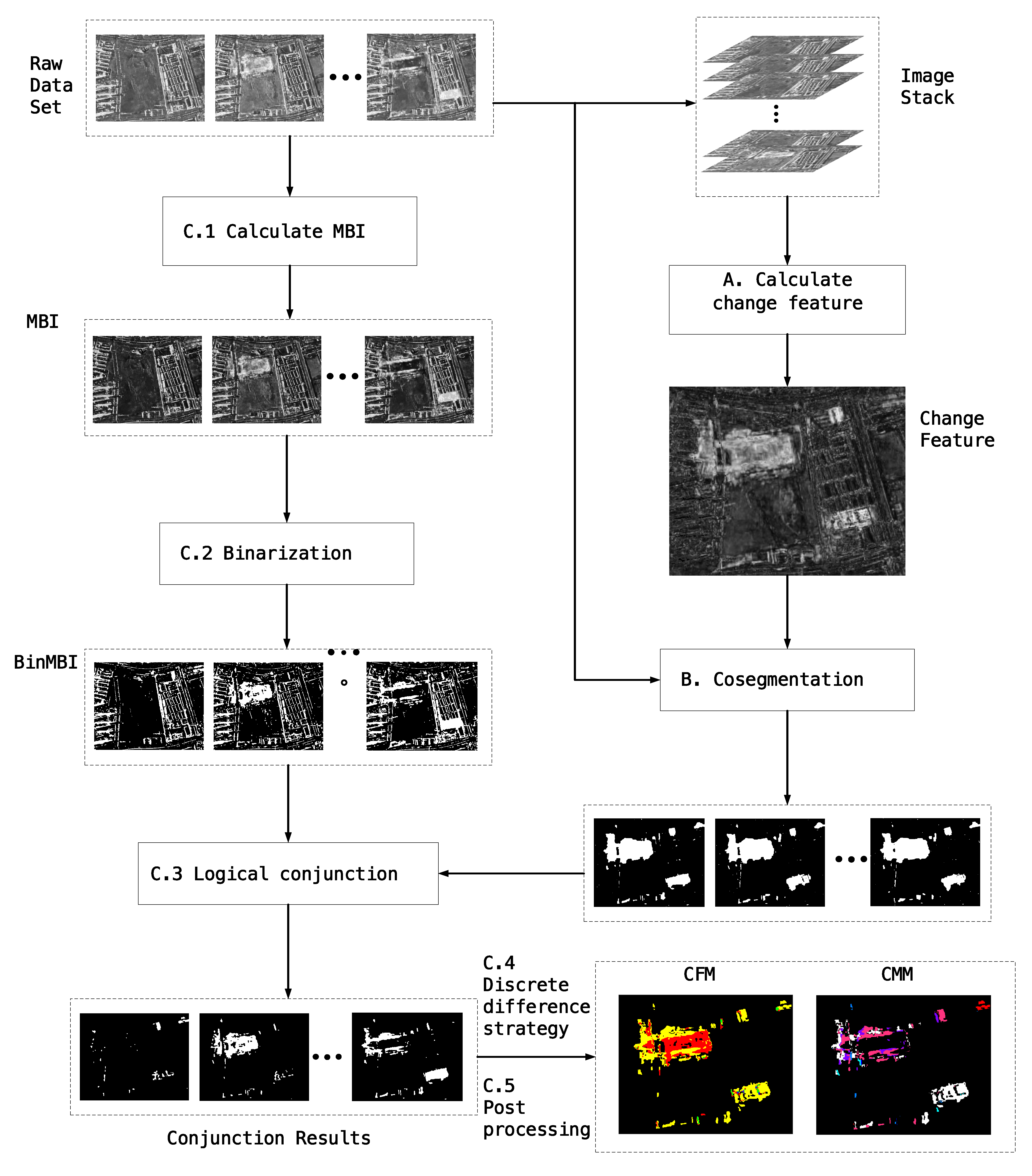
However, most multitemporal change detection approaches can only detect the change dynamics [11] or change classification [2,10,19]. Change classification has been explained above. Change dynamics in their paper is the probability of “changed” responses. The typologies of changes in our study include constructions, demolition and major displacements of buildings. Concretely, the constructions of buildings include analysis of the evolution of urbanization, monitoring for illegal construction, etc. The demolition and major displacements of buildings mainly involve urban redevelopments. In this paper, we propose a multitemporal change detection method that can acquire change frequency map and change moment maps. This proposed method is based on two hypotheses. (i) We assume that all the images have sufficient registration accuracy. (less than 0.5 pixel) (ii) The view angles of the sensors are almost the same. In other words, we do not consider changes caused by different view angles of the sensors. The details of our approach are as follows. Firstly, the change feature is generated using the proposed index. Meanwhile, MBI is calculated and binarized for each image. Secondly, the cosegmentation [17] is presented on each image and generate segmentation results for each date. Finally, CFM and CMMs are derived using cosegmentation results and binarized MBI.

For ease of expression, we first give explanations of CFM and CMMs.

1.1. Change Frequency Map (CFM)

An $r\times c$ matrix is said to be $CFM$ if $CFM\in \{A\in {\mathbb{Z}}^{r\times c}|a_{ij}\ge 0\}$ and the change frequency $CF$ in $CFM$ illustrate the number of changes at the corresponding pixel. Where $\mathbb{Z}$ is the set of integers and $r\times c$ is the size of input image. Let N be the number of input images, and it is obvious that $0\le CF\le N-1$.

1.2. Change Moment Maps (CMMs)

We first define the maximum number of changes:

$$K=\underset{i,j}{\max }C{F}_{ij}.$$

CMMs contain ${\sum }_{k=1}^{K}k=K(K+1)/2$ maps. The element of a change moment map shows the moment of change. For example, if some objects whose $CF$ equals three, then we have three change moment maps exhibiting the first, the second, and the third moment of change, respectively.

The rest of this paper is organized as follows: in Section 2, the principle and algorithm of the proposed method are explained in detail. Section 3 exhibits the experimental results and discussion using realistic TerraSAR-X time-series images to demonstrate the effectiveness of the proposed method. Finally, conclusions are drawn in Section 5.

2. Materials and Methods

In this section, we will introduce our novel building change detection framework in detail. The input of our algorithm is N registered SAR images. The basic idea of our method is to combine the changed area and the building area. In order to acquire the changed area, we proposed the change feature generator. However, the change feature generator is a pixel-level detector, which does not take into account neighborhood information. Accordingly, we use cosegmentation method proposed in [17] to make use of both change feature and neighborhood information. The cosegmentation method was firstly applied in binary-date change detection based on optical images. We modify the cosegmentation method and apply it in time-series SAR change detection. In the meanwhile, we extract building area using the MBI method. We finally combine the changed area and building area using a simple AND (logical conjunction) operation.

The workflow of our method is depicted in Figure 1.

Figure 1. The workflow of the proposed method.

2.1. Change Feature Generator

The change feature generator is used to generate difference map at pixel level. Change feature $I_C$ represents the severity of the change at pixel level. Let $\mathit{x}=\left[x_1,x_2,\dots ,x_N\right]$ represent one pixel values of N times. Therefore, the generator is to find a suitable index to measure the variation of $\mathit{x}$. In this paper, we give four indices, range R, variance ${\sigma }^2$, omnibus test Q [12] and max ratio L.

The range of x is the difference between the largest and smallest values:

$$I_{C1}=R=\max \left(\mathit{x}\right)-\min \left(\mathit{x}\right).$$

(1)

For binary-date change detection, i.e., $N=2$, $R=\left|x_2-x_1\right|$, which is equivalent to the classical difference detector.

The sample variance is a classic unbiased estimator to measure the variation of a set of values. The sample standard variance is defined as follows:

$$I_{C2}={\sigma }^2=\frac{{\sum }_{i=1}^N\left(x_i-\overline{x}\right)}{N-1}.$$

(2)

Q is derived from the omnibus test for equality of several complex covariance matrices [12]. In this paper, our data is single-band data and the number of looks equals one. In this case, Q is defined using the following equation:

$$Q=N^N\frac{{\prod }_{i=1}^N\left|x_i\right|}{{\left|x\right|}^N},$$

(3)

where $x={\sum }_{i=1}^N{x}_i$. If all the elements of x are equal, then $Q=1$. We use $I_{C3}=1-Q$ as change feature generator in this paper.

Similar to R, L is a simple extension of the classic ratio detector:

$$I_{C4}=L=\frac{\max \left(\mathit{x}\right)}{\min \left(\mathit{x}\right)}-1$$

(4)

Let T be the threshold of the change feature, and it can be calculated by expectation maximization(EM) algorithm [20].

As we can see from Equation (1) to Equation (4), $I_C$ reaches a minimum of zero if there is absolutely no change, then the normalization of $I_C$ equals to $\alpha I_C$($\alpha$ is a constant). Therefore, according to Equation (6), it does not matter whether $I_C$ is normalized because if T is the threshold of $I_C$, $\alpha T$ must be the threshold of $\alpha I_C$.

2.2. Cosegmentation

The workflow of cosegmentation strategy is depicted in Figure 2. The function of cosegmentation method is to segment an image into two parts using change feature based on graph theory. This segmentation result depends on change information and neighborhood information. Cosegmentation contains three following steps.

Figure 2. The workflow of cosegmentation strategy.

2.2.1. Graph Establishment

Graph establishment depends on the number of pixels of multitemporal images. For each image, we build a graph $G=\left(V,E\right)$, as shown in Figure 3. The graph contains three different kinds of nodes, which are source s, sink t, and normal nodes P, defined as follows:

$$V=P\cup \left\{s,t\right\}.$$

(5)

Figure 3. The graph structure of cosegmentation (adapted from [21]).

Node s and t represent background and foreground respectively. Every node in P represents a pixel of each image $I_i$. Every pixel node links with source s and sink t, which is called t-link, and they link their neighborhood pixels simultaneously, which is called n-link. An eight-neighborhood link is used in this experiment.

2.2.2. Edge Weight Setting

The edge weight of the graph depends on a manually set parameter and the pixel value of the change feature and raw image. In this paper, we adopt the weight setting method in [17] according to the edge weight setting principle, as Table 1 shown. Coefficient $\lambda$, which balances the relative importance between change feature information and neighborhood information, is set manually. The principle of weight set consists of three items.

Table 1. Edge weight setting.

Edge Type	Value	Condition
n-link($p,q$)	$\left(1-\lambda \right)V_{pq}$	$\left(p,q\right)\in N$
t-link($s,p$)	$\lambda D_f\left(I_C^p\right)$	$p\in P,I_C^p\le 2T$
	0	$p\in P,I_C^p>2T$
t-link($p,t$)	$\lambda D_b\left(I_C^p\right)$	$p\in P,I_C^p\le 2T$
	W	$p\in P,I_C^p>2T$

• Edges that link s and pixels that are more likely to change should be given a lower weight. Similarly, edges linking t and pixels that are more likely to change should be given higher weight. The other pixels do the opposite.
• For n-link, those edges linking similar pixels should be given higher weight. Edges linking significantly different pixels should be given a lower weight.
• For edges linking t and changed pixels, the weights should be significant enough to permit the flow to pass.

In Table 1, $I_C^p$ denotes the pixel value of $I_C$. The larger $I_C^p$, the more likely this pixel is to change. According to principle 1, we define $D_f\left(I_C^p\right)$ and $D_b\left(I_C^p\right)$:

$$\left\{\begin{array}{cc}{D}_f\left(I_C^p\right)=-\ln \left(\frac{I_C^p}{2T}\right),\hfill & \\ D_b\left(I_C^p\right)=-\ln \left(1-\frac{I_C^p}{2T}\right),\hfill \end{array}\right.$$

(6)

According to principle 2, we define $V_{pq}$.

$$\left\{\begin{array}{c}{V}_{pq}=\exp \left(-\frac{\parallel {\mathit{I}}_p-{\mathit{I}}_q{\parallel }^2}{2{\sigma }^2}\right)·\frac{1}{d\left(p,q\right)},\hfill \\ d\left(p,q\right)=\sqrt{{\left(r_p-r_q\right)}^2+{\left(c_p-c_q\right)}^2},\hfill \\ {\sigma }^2=\mathbb{E}\left[\parallel {\mathit{I}}_p-{\mathit{I}}_q{\parallel }^2\right]\hfill \end{array}\right.$$

(7)

where ${\mathit{I}}_p$ and ${\mathit{I}}_q$ represent pixel values (panchromatic) or the spectral feature vectors (multispectral) of pixel p and pixel q. $r_p$ and $c_p$ represent the row and column number of pixel p. $\mathbb{E}[·]$ means the average value of all neighborhood pixel pairs over the whole image. Finally, we can define W according to principle 3:

$$W=1+\underset{p\in P}{\max }\sum _{q\in N_8\left(p\right)}{V}_{pq}$$

(8)

where $N_8\left(p\right)$ is 8-neighbourhood of p.

2.2.3. Graph Cut

Graph cut aims to find a cut of this graph that serves:

$$\underset{C\in \Omega }{\min }\sum _{e\in C}{w}_e.$$

(9)

C is a cut of this graph, and e is an edge that belongs to C. $\Omega$ is the set of all cuts. $w_e$ is the weight of e. The energy minimization method [21] is adopted in this study to solve the graph cut problem.

2.3. Morphological Building Index

In this subsection, we give a review of the MBI method. MBI can extract buildings based on morphological processing, which was first used in optical images and achieved good results [18]. The basic idea of MBI is to build the relationship between the spectral-structural characteristics of buildings and the morphological operators. These spectral-structural characteristics of buildings are represented using the opening by reconstruction with a series of linear structural elements (SE). Let l and d, which are hyper-parameters set by traversing different values, denote length(pixel) and direction(degree) of linear SE, respectively. The d is generally constant and the l depends on the resolution of the image. The higher the resolution, the more pixels the building occupies, and l should be larger.

Buildings generally appear as high-brightness square objects in SAR images. The intuitive idea is to enhance these high-brightness square objects and in SAR images and suppress other parts of the image. Based on this idea, four characteristics are considered in this research: brightness, local contrast, size and directionality.

MBI calculation can be implemented by the following steps:

• Calculation of brightness of every pixel x.

  $$\beta \left(x\right)=\underset{1\le b\le B}{\max }\left(ban{d}_b\left(x\right)\right)$$
• White top-hat by reconstruction (WTH):

  $$WTH\left(d_i,l_j\right)=\beta -{\gamma }_b^{re}\left(d_i,l_j\right)$$

  where represents the opening-by-reconstruction [22] of the brightness image, and and l and d are two series that indicate the length and direction of a linear structural element, respectively. The parameters l and d in this research are displayed in Table 2. We use $d_i$ and $l_j$ to represent the ith ($1\le i\le i_m$) and jth ($1\le j\le j_m$) number of d and l. As shown in Table 2, $i_m$ equals 5 and $j_m$ equals 4.
  Table 2. Parameter setting.

  Step	Parameter	Value
  MBI calculation	l	$[0,50,100,150,200]$
  	d	$[0,60,120,180]$
  cosegmentation	$\lambda$	0.25

• Morphological profiles (MP):

  $$M{P}_{WTH}\left(d_i,l_j\right)=WTH\left(d_i,l_j\right)$$
• Differential morphological profiles (DMP): The DMP of the white top-hat is defined as:

  $$DM{P}_{WTH}\left(d_i,l_j\right)=|M{P}_{WTH}\left(d_i,l_j\right)-M{P}_{WTH}\left(d_i,l_{j-1}\right)|$$
  We define $M{P}_{WTH}\left(d_i,l_0\right)=\beta$.
• Finally, the morphological building index (MBI) is defined as the average of DMP:

  $$MBI=\frac{{\sum }_{i,j}DM{P}_{WTH}\left(d_i,l_j\right)}{i_m\times j_m}$$

2.4. Extract Change Information

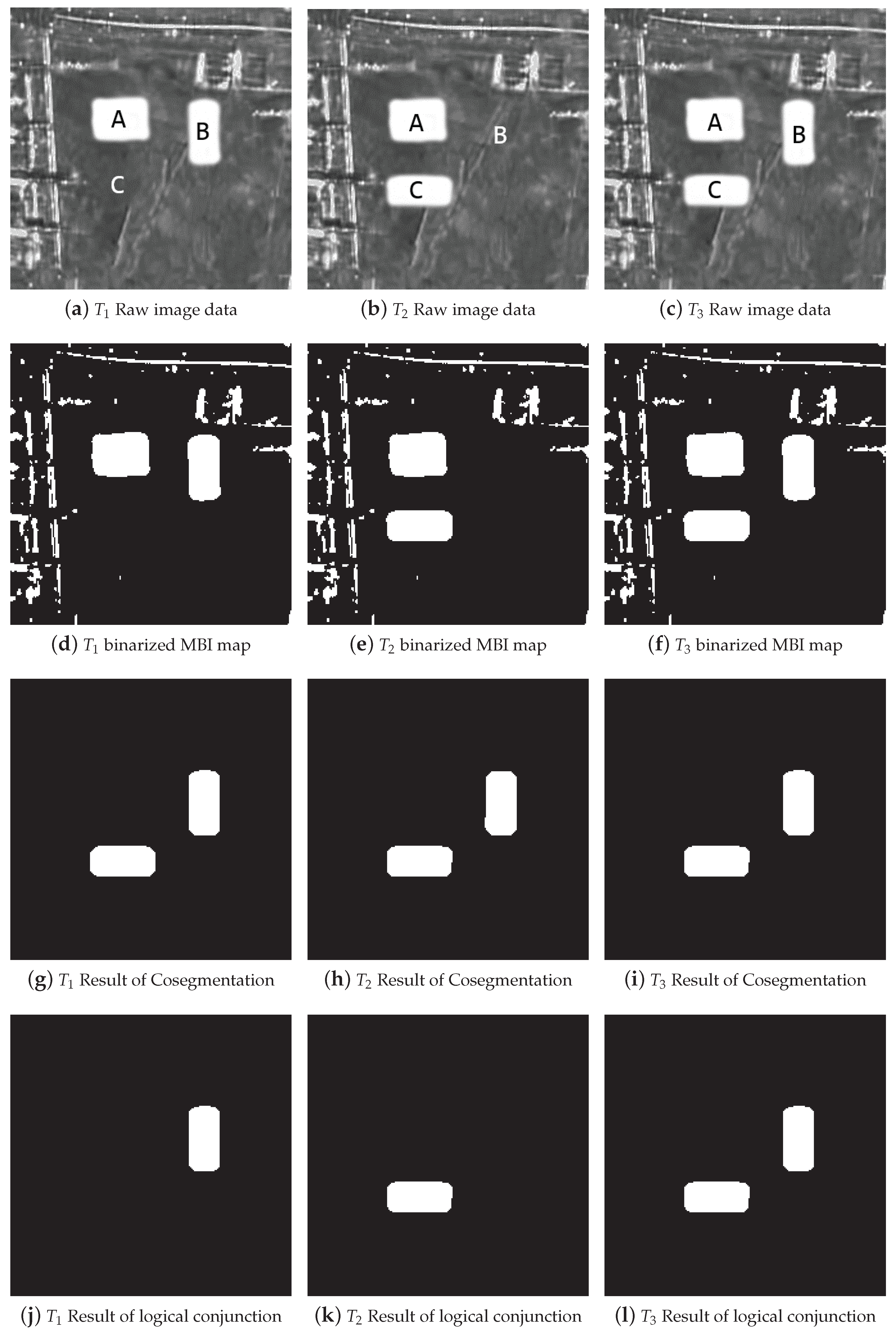
Cosegmentation can not detect when one object exists or disappears. Assume a building existed on $T_1$, demolished on $T_2$, and rebuilt at the same place on $T_3$. Under this circumstance, the results of the cosegmentation method are almost the same on each time, as shown in Figure 4g–i.

Figure 4. Synthetic data. For contrast, we test three regions, names A, B, and C. The building in region A did not change. The building in region B was demolished on time 2, and a new building was constructed on time 3. The building in region C was constructed on time 2 and did not change on time 3.

In order to solve this problem, we propose an extraction method, corresponding to C.1 to C.5 in Figure 1.

Precisely, we first calculate the MBI map and binarize the MBI map using OTSU [23], which are depicted in Figure 4d–f. Finally, we make logical conjunction between binMBI and cosegmentation results. The logical conjunction results illustrate when the objects exist or disappear, as shown in Figure 4j–l. With this logical conjunction results, we can easily detect change frequency and change moments for each pixel using a discrete difference strategy. Furthermore, the post-processing is to remove small fragments that are less than 100 m².

In general, extraction consists of three steps. (1) Generating building objects using the MBI index. (2) Intersecting binMBI and cosegmentation result to extract change building objects each time. (3) Counting change moment for each building objects and recognize when they change. The extraction procedure can be summarized in Algorithm 1.

Algorithm 1 Extracting change times map and change moments sequence map.

Input:

Raw Image Data, $\mathit{I}=\left\{I_1,I_2,\dots ,I_N\right\}$;

Cosegmentation Result, $\mathit{S}=\left\{S_1,S_2,\dots ,S_N\right\}$;

Output:

Change Frequency Map, $CFM$;

Change Moments Map $CMM$;

1: $\mathit{M}={\mathit{f}}_{MBI}\left(\mathit{I}\right)$ $\mathit{M}=\left\{M_1,M_2,\dots ,M_N\right\}$;

2: ${\mathit{M}}_b={\mathit{f}}_{OSTU}\left(\mathit{M}\right)$;

3: for $i=1:N$ do

4:  $S_i=M_i\cap S_i$;

5:  Close and open operation for $S_i$;

6: end for

7: $D_i=S_{i+1}-S_{i}i=1,2,\dots ,N-1$

8: Removing small fragments in $D_i$

9: $CFM={\sum }_{i=1}^{N-1}{D}_i$

10: return $CFM$

11: Let $k=\max \left(CFM\right)$

12: for $i=1:K$ do

13:  for $j=1:i$ do

14:   Recognizing the moment of jth change for each object that changed i times in total;

15:  end for

16: end for

17: return $CMM$;

In step 5, We first adopt a morphological closing operation with a square structural element of 3 × 3 pixels to fill gaps and then adopt a morphological opening operation with the same structural element for smoothing.

In step 8, fragments remove procedure is removing small objects whose area is less than 100 m², which may be caused by noise.

The output of Algorithm 1 consists of a change times map $CFM$ and $\frac{K(K+1)}{2}$ change moment maps $CMM$.

3. Experiment

3.1. Accuracy Assessment

In binary-date change detection, the image is divided into changed and unchanged areas, which can be seen as a binary classification problem. However, in time-series change detection, the change frequency classification is not equivalent to common multi-classification problems. Assume that the real change frequency $f=5$, and the outputs of the two detectors equal 6 and 8 respectively. It is obvious that the first detector is superior, but the assessment index of the common classification problem cannot distinguish the two detectors.

In order to quantitatively verify the performance and effectiveness of our method, we propose a novel assessment index average change difference(ACD) for CFM accuracy assessment. Let Y denote the real CFM and $\widehat{Y}$ denote the output CFM of the detector. The ACD is defined as follows:

$$ACD=\frac{1}{rc}\sum _{i=1}^r\sum _{j=1}^c|{\widehat{Y}}_{ij}-Y_{ij}|.$$

(10)

Furthermore, we could only consider changed areas, then we define a mask M that denotes real changed areas:

$$\left\{\begin{array}{cc}{M}_{ij}=1,Y_{ij}\ge 1\hfill & \\ M_{ij}=0,else\hfill \end{array}\right.$$

(11)

More generally, we define mask $M^k$ that denotes areas where $f\ge k$:

$$\left\{\begin{array}{cc}{M}_{ij}^k=1,Y_{ij}\ge k\hfill & \\ M_{ij}^k=0,else\hfill \end{array}\right.$$

(12)

Then the mask ACD can be defined as follows:

$$AC{D}^k=\frac{{\sum }_{i=1}^r{\sum }_{j=1}^c|{\widehat{Y}}_{ij}-Y_{ij}|M_{ij}^k}{{\sum }_{i=1}^r{\sum }_{j=1}^c{M}_{ij}^k}.$$

(13)

The ACD denotes the expectation of the absolute error of a change detector. It is obvious that the smaller ACD is, the better detector. ACD equals zero if and only if $\widehat{Y}=Y$.

3.2. Dataset

In this paper, the study area is located in Tongzhou District of Beijing. Tongzhou has been undergoing rapid changes over the past ten years. Two TerraSAR-X datasets with 0.9 m range resolution and 1.8 m azimuth resolution are used in our experiment. The first dataset, obtained from Jan. 2012 to May 2013, contains eight images with $400\times 500$ size, and the second dataset contains 16 images with $501\times 451$ size acquired from Jan. 2012 to Mar. 2016. The construction and demolition of buildings in this area shown in data 1 are conducive to validating the effectiveness of different change detection algorithms. In the area shown in data 2, many small houses were gradually built from north to south from 2012 to 2016. This region is a typical example of the process of urbanization, which can be clearly illustrated in $CM{M}_{11}$ in Figure 7.

Raw data should be preprocessed before change detection. We first implement radiometric calibration and co-registration. Then we adopt MSAR-BM3D [24] for denoising. MSAR-BM3D method obtains an excellent despeckling capability in the spatial dimension, which is effective for dealing with multitemporal data. As shown in Figure A1 The sample denoised images and the corresponding optical images are displayed in Figure 5.

Figure 5. The two time-series dataset of TerraSAR-X remote sensing images in the Tongzhou District of Beijing. (a) The 7th scene of the first dataset and the corresponding optical image is shown in (b). (c) The 10th scene of the second dataset and the closest optical image in time is shown in (d).

3.3. Parameter Setting

To our knowledge, our framework is the first simultaneous comparison method to generate CFM and CMMs. However, we can simply modify some other similar methods to make a contrast experiment. The statistical features and temporal clustering (SFTC) [2] and NORCAMA [10] are designed for change classification, which can be modified to generate CFM and CMMs. In the experiments, our method was compared with these two multitemporal change detection methods to demonstrate its superiority. There are two steps requiring manual parameter setting, the MBI calculation step and cosegmentation step. The parameter setting is shown in Table 2. In the cosegmentation step, $\lambda$ is set by $0.25$, which is a great balance between changing feature information versus neighborhood information.

3.4. Results

In this section, we present the accuracies for different methods using two datasets. We neglect $AC{D}^k$ for $k\ge 3$ because objects whose $CF\ge 3$ play a small part (0.94% in data 1 and 5.7% in data 2) and we do not have to consider it in isolation. The ACD of the two datasets is depicted in Figure 8.

The CFM and part of CMMs of the two datasets are illustrated in Figure 6 and Figure 7. For the sake of argument, we define the following symbol:

$$CM{M}_{ij}i\ge j\ge 1,$$

(14)

where $CM{M}_{ij}$ indicates the jth change moment for those objects whose $CF=i$. For example, $CM{M}_{11}$ means the first moment of change for objects whole change frequency equals 1.

Figure 6. Four images of original data 1 (after denoising) are illustrated in the first line. The second line displays the change frequency map (CFM) and change moment maps (CMMs) of data 1. To conserve space, we only illustrate CMMs of objects whose $CF\le 2$ because very few objects change more than three times.

Figure 7. Four images of original data 2 (after denoising) are illustrated in the first line. The second line displays the CFM and CMMs of data 2. To conserve space, we only illustrate CMMs of objects whose $CF\le 2$ because very few objects change more than three times.

Some sample images of the first dataset are shown in Figure 6. In Figure 6b, the objects in area 1 were constructed in $T_6$, and were demolished in $T_8$ so that the $CF$ of these objects equals 2. The $CF$ of other objects in area 2, also equals to 2, but they were constructed in $T_7$ and demolished in $T_8$. These two types of objects were built at different times but dismantled at the same time. Therefore, the $CF$ and $CM{M}_{22}$ of these two types of objects are the same while the $CM{M}_{21}$ is different. The experiment of dataset 1 demonstrates the effectiveness of CMMs for detecting when the objects are built and when they are demolished.

In the first line of Figure 7, we select four representative images from the second dataset. From 2012 to 2016, these small bungalows began to be built gradually from north to south, which is a typical change detection task. The CFM indicates the change frequency of the area of interest. What we found from CFM is that most objects changed only once and a small part of objects changed twice or more. $CM{M}_{11}$ exhibits the construction process of these bungalows in this area. In $CM{M}_{11}$, the different change moments are represented in different colors, where we can see that these bungalows are built from north to south gradually.

The different values K generated by different methods are listed in Table 3.

Table 3. The different values K generated by different methods.

	Dataset 1	Dataset 2
NORCAMA	7	15
SFTC	4	4
Proposed-R	5	5
Proposed-${\sigma }^2$	5	8
Proposed-Q	5	6
Proposed-L	5	6
Ground truth	4	5

We only illustrate CMMs of objects whose $CF\le 2$ in Figure 6 and Figure 7 because very few objects change more than three times. The $CM{M}_{31}$, $CM{M}_{32}$ and $CM{M}_{33}$ of these two datasets are illustrated in the appendix, as shown in Figure A2 and Figure A3. Experimental results contain plenty of figures so that we put them in the Appendix A, which is also available on https://github.com/txdtplus/zhang2020_appendix. This website includes CFM, CMMs, and illustrations of two datasets.

4. Discussion

4.1. Data Applicability

This method is specially designed for single polarized SAR images. Changes in vegetation are not evident in SAR images, which is very helpful for building change detection. However, in optical images, we have to extract the building areas using NDVI or other indices before detecting building changes. For multispectral optical images or multi-polarization SAR images, we need to find new ways to generate change feature.

4.2. Accuracy

Compared to other methods, our framework is designed especially for multitemporal building change detection and generating CFM and CMMs. The core of our framework is the contact between MBI calculation and cosegmentation. As Figure 8 shows, the change feature generator selection has little effect on accuracy. Figure 9 and Figure 10 show different CFMs generated by various methods, which illustrate qualitative results comparing with other methods. The quantitative results of the various methods are list in Table 4 and Table 5, as well as in Figure 8.

Figure 8. Average change difference (ACD) results of each dataset. The red font denotes the best method under this assessment index.

Figure 9. CFM of different methods using data 1.

Figure 10. CFM of different methods using data 2.

Table 4. Numerical results of the various methods using data 1.

	NORCAMA	SFTC	Proposed-R	Proposed-${\mathit{\sigma }}^2$	Proposed-Q	Proposed-L
$AC{D}^0$	0.336	0.082	0.047	0.063	0.047	0.035
$AC{D}^1$	1.394	0.708	0.188	0.186	0.177	0.195
$AC{D}^2$	1.303	1.004	0.214	0.228	0.219	0.229
Calculating Time	44.02 s	2.32 s	6.91 s	6.37 s	6.69 s	6.33 s

Table 5. Numerical results of the various methods using data 2.

	NORCAMA	SFTC	Proposed-R	Proposed-${\mathit{\sigma }}^2$	Proposed-Q	Proposed-L
$AC{D}^0$	1.973	0.211	0.180	0.183	0.177	0.180
$AC{D}^1$	4.375	0.969	0.694	0.699	0.758	0.771
$AC{D}^2$	3.771	2.055	1.244	1.281	1.441	1.382
Calculating Time	57.54 s	3.84 s	16.31 s	15.06 s	15.89 s	16.83 s

The detection errors are mainly caused by building recognition step and despeckling step. As shown in Figure A1, the boundaries of the adjacent small buildings become more blurred after despeckling, which poses a greater challenge to building recognition.

4.3. Algorithm Complexity

MBI calculation takes up most of the time of the algorithm. We implement experiments on a computer with i5 CPU at 3.00 GHz (6 cores) and 16 GB RAM. The runtimes of the three methods are listed in Table 4 and Table 5.

5. Conclusions

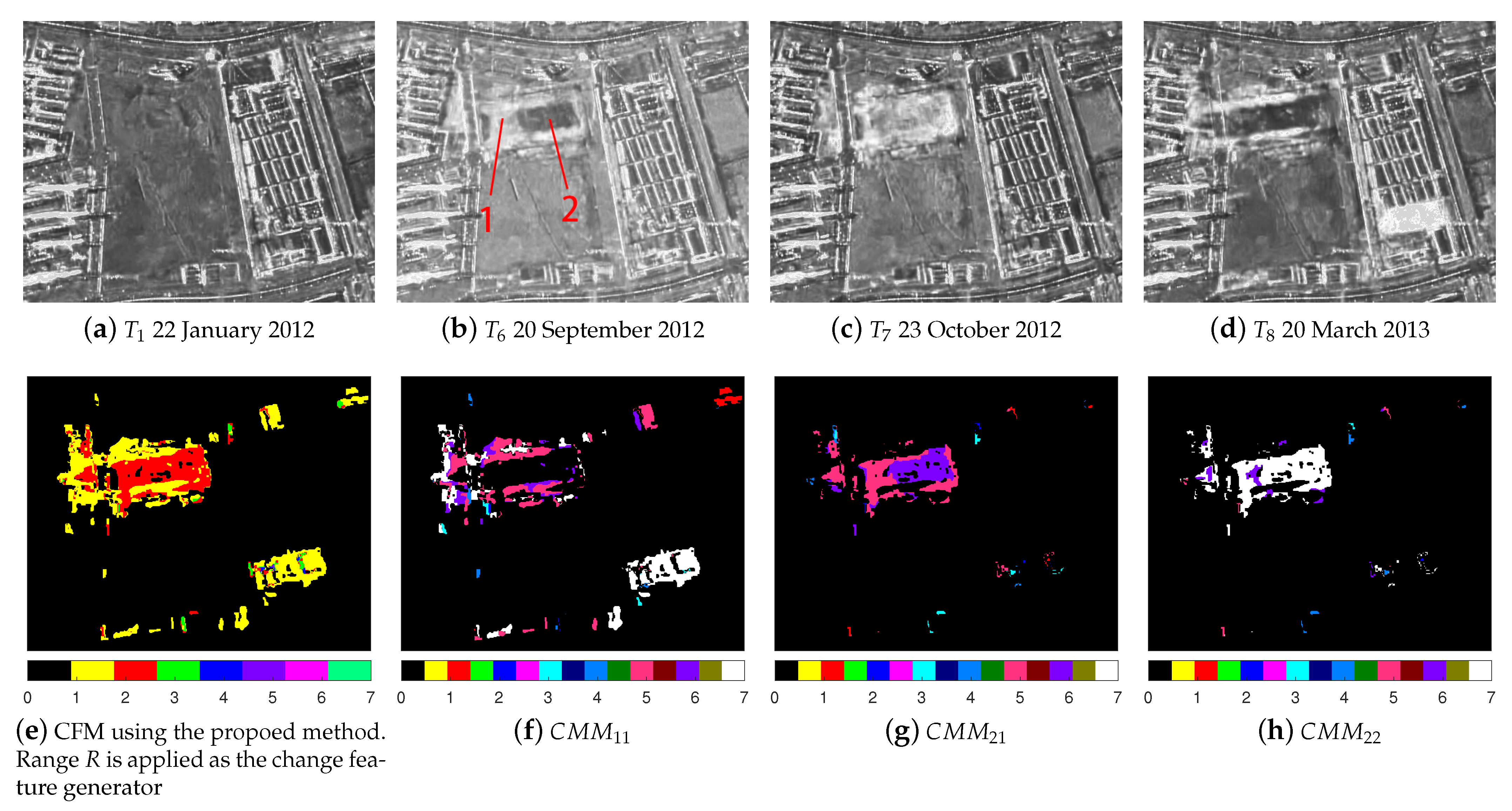
We propose a novel multitemporal building change detection framework that can generate change frequency map(CFM) and change moment maps(CMMs) from multitemporal SAR images. We first give definitions of CFM and CMMs, then a new cosegmentation based on multitemporal images and change feature generator is proposed to divide time-series images into changed and unchanged areas separately. The proposed cosegmentation and the morphological building index(MBI) are combined to extract changed building objects. The logical conjunction between the cosegmentation results and the binarized MBI is performed to recognize every moment of change. In the post-processing step, we use fragment removal to increase accuracy. Finally, we propose a novel accuracy assessment index for CFM.

The proposed method can acquire both CFM and CMMs while most multitemporal change detection approaches only capture the intensity of change. CFM and CMMs are of great significance to the field of building change monitoring. The experiment of dataset 1 demonstrates the effectiveness of CMMs for detecting when the objects are built and when they are demolished. The experiment on the second dataset illustrates that the CMMs can clearly state the process of urban building expansion.

The accuracy of our method is superior to other methods under the ACD index. We first introduce the cosegmentation method into an unsupervised multi-temporal SAR image change detection field and acquire excellent results. Both synthetic data and real TerraSAR-X data demonstrate the effectiveness of our method.

Appendix A.1

The appendix contains $CM{M}_{3j}(j=1,2,3)$ and $CM{M}_{4j}(j=1,2,3,4)$ of these two datasets, as shown in Figure A2 and Figure A3. The $CM{M}_{ij}(i>4)$ include so few objects that we do not put them in this article. The whole experimental results is also available on https://github.com/txdtplus/zhang2020_appendix. This website includes CFM, CMMs, and illustrations of two datasets.

Appendix A.2. An Example of Denoising Using MSAR-BM3D

Figure A1. An image before (a) and after (b) despeckling by MSAR-BM3D.

Figure A2. CMMs $\left(CF=3\right)$.

Figure A3. CMMs $\left(CF=4\right)$.

References

- Lu, D.; Mausel, P.; Brondizio, E.; Moran, E. Change detection techniques. Int. J. Remote Sens. 2004, 25, 2365–2401. [Google Scholar] [CrossRef]
- Yuan, J.; Lv, X.; Dou, F.; Yao, J. Change Analysis in Urban Areas Based on Statistical Features and Temporal Clustering Using TerraSAR-X Time-Series Images. Remote Sens. 2019, 11, 926. [Google Scholar] [CrossRef]
- Hu, Y.; Dong, Y. An automatic approach for land-change detection and land updates based on integrated NDVI timing analysis and the CVAPS method with GEE support. ISPRS J. Photogramm. Remote Sens. 2018, 146, 347–359. [Google Scholar] [CrossRef]
- Chen, X.; Chen, J.; Shi, Y.; Yamaguchi, Y. An automated approach for updating land cover maps based on integrated change detection and classification methods. ISPRS J. Photogramm. Remote Sens. 2012, 71, 86–95. [Google Scholar] [CrossRef]
- Zhang, X.; Xiao, P.; Feng, X.; Yuan, M. Separate segmentation of multi-temporal high-resolution remote sensing images for object-based change detection in urban area. Remote Sens. Environ. 2017, 201, 243–255. [Google Scholar] [CrossRef]
- Wang, X.; Liu, S.; Du, P.; Liang, H.; Xia, J.; Li, Y. Object-based change detection in urban areas from high spatial resolution images based on multiple features and ensemble learning. Remote Sens. 2018, 10, 276. [Google Scholar] [CrossRef]
- Anniballe, R.; Noto, F.; Scalia, T.; Bignami, C.; Stramondo, S.; Chini, M.; Pierdicca, N. Earthquake damage mapping: An overall assessment of ground surveys and VHR image change detection after L’Aquila 2009 earthquake. Remote Sens. Environ. 2018, 210, 166–178. [Google Scholar] [CrossRef]
- Janalipour, M.; Taleai, M. Building change detection after earthquake using multi-criteria decision analysis based on extracted information from high spatial resolution satellite images. Int. J. Remote Sens. 2017, 38, 82–99. [Google Scholar] [CrossRef]
- Washaya, P.; Balz, T.; Mohamadi, B. Coherence change-detection with sentinel-1 for natural and anthropogenic disaster monitoring in urban areas. Remote Sens. 2018, 10, 1026. [Google Scholar] [CrossRef]
- Su, X.; Deledalle, C.; Tupin, F.; Sun, H. NORCAMA: Change analysis in SAR time series by likelihood ratio change matrix clustering. Isprs J. Photogramm. Remote Sens. 2015, 101, 247–261. [Google Scholar] [CrossRef]
- Le, T.T.; Atto, A.M.; Trouve, E. Change analysis using multitemporal Sentinel-1 SAR images. In Proceedings of the 2015 IEEE International Geoscience and Remote Sensing Symposium (IGARSS), Milan, Italy, 26–31 July 2015; pp. 4145–4148. [Google Scholar]
- Conradsen, K.; Nielsen, A.A.; Skriver, H. Determining the Points of Change in Time Series of Polarimetric SAR Data. IEEE Trans. Geosci. Remote Sens. 2016, 54, 3007–3024. [Google Scholar] [CrossRef]
- Nascimento, A.D.C.; Frery, A.C.; Cintra, R.J. Detecting Changes in Fully Polarimetric SAR Imagery With Statistical Information Theory. IEEE Trans. Geosci. Remote Sens. 2019, 57, 1380–1392. [Google Scholar] [CrossRef]
- Mian, A.; Ginolhac, G.; Ovarlez, J.; Atto, A.M. New Robust Statistics for Change Detection in Time Series of Multivariate SAR Images. IEEE Trans. Signal Process. 2019, 67, 520–534. [Google Scholar] [CrossRef]
- Cavalagli, N.; Kita, A.; Falco, S.; Trillo, F.; Costantini, M.; Ubertini, F. Satellite radar interferometry and in-situ measurements for static monitoring of historical monuments: The case of Gubbio, Italy. Remote Sens. Environ. 2019, 235, 111453. [Google Scholar] [CrossRef]
- Del Soldato, M.; Solari, L.; Poggi, F.; Raspini, F.; Tomás, R.; Fanti, R.; Casagli, N. Landslide-Induced Damage Probability Estimation Coupling InSAR and Field Survey Data by Fragility Curves. Remote Sens. 2019, 11, 1486. [Google Scholar] [CrossRef]
- Xiao, P.; Yuan, M.; Zhang, X.; Feng, X.; Guo, Y. Cosegmentation for object-based building change detection from high-resolution remotely sensed images. IEEE Trans. Geosci. Remote Sens. 2017, 55, 1587–1603. [Google Scholar] [CrossRef]
- Huang, X.; Zhang, L. Morphological building/shadow index for building extraction from high-resolution imagery over urban areas. IEEE J. Sel. Top. Appl. Earth Obs. Remote Sens. 2011, 5, 161–172. [Google Scholar] [CrossRef]
- Saha, S.; Bovolo, F.; Bruzzone, L. Building Change Detection in VHR SAR Images via Unsupervised Deep Transcoding. IEEE Trans. Geosci. Remote Sens. 2020. [Google Scholar] [CrossRef]
- Bruzzone, L.; Prieto, D.F. Automatic analysis of the difference image for unsupervised change detection. IEEE Trans. Geosci. Remote Sens. 2000, 38, 1171–1182. [Google Scholar] [CrossRef]
- Boykov, Y.; Kolmogorov, V. An experimental comparison of min-cut/max-flow algorithms for energy minimization in vision. IEEE Trans. Pattern Anal. Mach. Intell. 2004, 26, 1124–1137. [Google Scholar] [CrossRef]
- Gonzalez, R.C.; Woods, R.E. Digital Image Processing, 3rd ed.; Pearson Prentice Hall: Upper Saddle River, NJ, USA, 2006; p. 659. [Google Scholar]
- Otsu, N. A threshold selection method from gray-level histograms. IEEE Trans. Syst. Man, Cybern. 1979, 9, 62–66. [Google Scholar] [CrossRef]
- Chierchia, G.; El Gheche, M.; Scarpa, G.; Verdoliva, L. Multitemporal SAR image despeckling based on block-matching and collaborative filtering. IEEE Trans. Geosci. Remote Sens. 2017, 55, 5467–5480. [Google Scholar] [CrossRef]
Publisher’s Note: MDPI stays neutral with regard to jurisdictional claims in published maps and institutional affiliations. |
© 2021 by the authors. Licensee MDPI, Basel, Switzerland. This article is an open access article distributed under the terms and conditions of the Creative Commons Attribution (CC BY) license (http://creativecommons.org/licenses/by/4.0/).