Modelling Daily Gross Primary Productivity with Sentinel-2 Data in the Nordic Region–Comparison with Data from MODIS

Abstract

The high-resolution Sentinel-2 data potentially enable the estimation of gross primary productivity (GPP) at finer spatial resolution by better capturing the spatial variation in a heterogeneous landscapes. This study investigates the potential of 10 m resolution reflectance from the Sentinel-2 Multispectral Instrument to improve the accuracy of GPP estimation across Nordic vegetation types, compared with the 250 m and 500 m resolution reflectance from the Moderate Resolution Imaging Spectroradiometer (MODIS). We applied linear regression models with inputs of two-band enhanced vegetation index (EVI2) derived from Sentinel-2 and MODIS reflectance, respectively, together with various environmental drivers to estimate daily GPP at eight Nordic eddy covariance (EC) flux tower sites. Compared with the GPP from EC measurements, the accuracies of modelled GPP were generally high (R² = 0.84 for Sentinel-2; R² = 0.83 for MODIS), and the differences between Sentinel-2 and MODIS were minimal. This demonstrates the general consistency in GPP estimates based on the two satellite sensor systems at the Nordic regional scale. On the other hand, the model accuracy did not improve by using the higher spatial-resolution Sentinel-2 data. More analyses of different model formulations, more tests of remotely sensed indices and biophysical parameters, and analyses across a wider range of geographical locations and times will be required to achieve improved GPP estimations from Sentinel-2 satellite data.

1. Introduction

Atmospheric carbon dioxide (CO₂) from anthropogenic emissions is one of the key drivers of climate change [1]. The techniques used to quantify land–atmosphere carbon exchanges are essential for the understanding of the global carbon cycle [2]. Especially Northern land ecosystems play an important role in the global carbon cycle due to the high amount of carbon stored in boreal ecosystems [3] and the increasing seasonal CO₂ exchange [4]. Micrometeorological eddy covariance (EC) measurements, conducted at fixed towers, can provide in situ estimates of CO₂ exchange at the ecosystem level, from which Gross Primary Productivity (GPP) can be estimated [5]. However, these measurements lack the spatial coverage needed for the characterization of CO₂ fluxes at larger regional extents (10³–10⁶ km²), and to represent different age classes and species diversity [6].

An efficient way to estimate GPP across larger areas is to use observations from Earth observation satellites. Satellite-derived approaches for carbon modelling are usually based on the light use efficiency (LUE) model [7], empirical models with site- or ecosystem-specific environmental variables [8], or mechanistic models with remotely sensed inputs [9,10,11]. LUE models express GPP as a product of the photosynthetic light use efficiency (ε), and photosynthetically active radiation absorbed by the vegetation (APAR). Although APAR is nonlinearly correlated to GPP at the daily time step [12,13], the relationship can be considered linear over monthly or annual periods [14,15,16]. APAR can be derived by multiplying PAR (photosynthetically active radiation) by fAPAR (fractional PAR absorbed by the vegetation). Several studies have shown that satellite-derived spectral vegetation indices have linear or near-linear relationships with fAPAR within different vegetation types and climatic conditions and are therefore used as proxies of fAPAR [17,18,19,20]. The LUE factor, on the other hand, is more difficult to estimate. LUE models usually rely on biome-specific maximum LUE factors that are reduced due to environmental constraints such as air temperature and water content [21,22,23]. However, meteorological data and a biome-specific maximum LUE factor might be too coarse to accurately describe spatial and temporal variations of the LUE factor [11,22,24]. Due to this issue, empirical models based on remotely sensed input have been developed for estimating terrestrial GPP [25,26,27]. In these models the regression parameter represents the LUE factor since it scales fAPAR to the level of carbon assimilation. The simplest empirical models use only a vegetation greenness index such as the Normalized Difference Vegetation Index (NDVI) proposed by Tucker [28] or the Enhanced Vegetation Index (EVI) proposed by Huete et al. [20] to estimate GPP. In comparison to the widely used NDVI, EVI is more adjustable for reducing soil and atmospheric effects and more sensitive to structural variations in vegetation [20]. The further developed two-band Enhanced Vegetation Index (EVI2) provides similar information on vegetation properties to EVI but only uses the red and near-infrared bands, whereas EVI also requires the blue band [29]. However, Sims et al. [24] showed that a model based entirely on EVI only poorly explains the seasonal variation of GPP at sites with evergreen vegetation that experience summer drought. Especially in boreal forests the air temperature (T_a) and the availability of light (PAR) regulate the seasonal photosynthetic activity [30]. In addition, summer drought is typically the result of high T_a and increased vapor pressure deficit (VPD) [31]. Consequently, including PAR, T_a and VPD variables in the model along with a remotely sensed vegetation index is assumed to improve the GPP estimation.

When calibrating remote sensing models against EC CO₂ data, it should be noted that the EC data represent large exchange areas, roughly covering a distance of 10 to 100 times the height of the measurements over displacement height [32,33]. The area influencing the measured flux is called the source area [34], the contribution of each part to the measured flux (source weight) is called the flux footprint, and it depends on wind direction, wind speed and turbulence, leading to the variation of footprint from one half-an-hour flux averaging period to another [35]. The rough approximation above disregards this variation in flux footprint, thus introducing scale and weather-dependent approximation errors [36,37]. For accurate spatial representation of flux variations, a footprint model should be used [38,39]. This type of model can be used to assess which pixels belong to the footprint and hence should be selected for the calibration.

To model GPP on local and global scales, data from the Moderate Resolution Imaging Spectroradiometer (MODIS) sensor on board NASA’s Terra and Aqua satellites have been widely used. Due to its high temporal resolution, MODIS provides data for monitoring vegetation dynamics and changes in land cover over time. However, MODIS acquires data at three relatively low spatial resolutions: 250 m, 500 m, and 1 km. The widely used MODIS GPP/NPP (MOD17, collection 6) product at 500 m spatial resolution has been questioned by many, mainly due to a lack of sufficient flux measurements for validation and calibration of the algorithm [40,41,42].

The spatial resolution of satellite products has been identified as a critical factor that limits spatially detailed carbon flux estimates, especially in heterogeneous landscapes [43]. The new Sentinel-2A and 2B satellites with the MultiSpectral Instrument (MSI) have great potential for studying CO₂ fluxes in terrestrial ecosystems due to improved spatial resolution (10 m, 20 m, and 60 m) and high temporal resolution (2–5 days’ revisit frequency depending on latitude). A few studies have explored the performance of the Sentinel-2 products for CO₂ flux modelling, e.g., Lin et al. [44] applied 30 m Sentinel-2 data from the Harmonized Landsat and Sentinel-2 product to estimate the GPP (R² = 0.77 and RMSE = 0.81 g C m⁻² day⁻¹ comparing to EC GPP) of three evergreen broadleaf forest sites and two grassland sites in southeast Australia. In the study by Wolanin et al. [45], Sentinel-2 and Landsat 8 data were used to estimate GPP (R² = 0.92 and RMSE = 1.38 g C m⁻² day⁻¹) on five crop fields (four in the USA and one in Germany). Given that Sentinel-2 has been shown to be capable of accurate representation of phenology [46,47] and has the capability to provide detailed estimates of biophysical and biochemical vegetation parameters [48,49] it can be hypothesized that Sentinel-2 MSI data has the potential to enhance the performance of GPP models also in northern landscapes. However, the impact of the lower temporal frequency of Sentinel-2 compared to MODIS in these high-cloudiness areas is a factor that could have negative impact.

In this study, we analyze eight study sites within the Nordic region (Denmark, Finland and Sweden, Figure 1) to investigate the accuracy of GPP estimates from Sentinel-2 data in comparison with MODIS data. We base the comparison on empirical regression models as they are commonly used for estimating GPP, and are functionally similar to the LUE type models. Following this, we examine the relationships between EC-derived GPP and EVI2-derived GPP using EVI2 and meteorological variables. In investigating the potential of Sentinel-2 vegetation index data for modeling carbon uptake, the study aims to (1) examine the effects of using Sentinel-2 MSI 10-m data compared to MODIS 250 m and 500 m data on modeling GPP from EC measurements, and (2) determine the importance of the input data for modeling accuracy in comparison to the choice of environmental driving variables.

2. Materials and Methods

2.1. Study Sites and Environmental Variables

The study area contains eight EC flux sites located in Denmark, Finland and Sweden, at latitudes from 55° N to 68° N (Figure 1). The flux sites belong to the ICOS infrastructure (https://www.icos-ri.eu) and follow the ICOS measurement protocols [50]. We analyzed data from 2016 to 2017, except at the SE-Svb site where we used only the data from 2016. There is an air-temperature gradient from south to north across the eight sites, with climate zones ranging from temperate in the south, through hemiboreal and boreal, and up to the northernmost subarctic landscapes. The sites cover diverse and major Nordic land cover types: evergreen forest, deciduous forest, wetlands, and agriculture (

Table 1. The eight ICOS flux tower sites used in this study. For more site information, refer to the national ICOS information pages (https://www.icos-ri.eu/).

Site Name	Site Name	Latitude (Degree)	Longitude (Degree)	Annual Average Ta (°C) 1	Flux Measurement Height (m)	Biome/Vegetation
SE-Sto	Abisko-Stordalen	68.36	19.05	0.5	2	Subarctic mire
SE-Svb	Svartberget	64.25	19.77	2.9	33	Boreal mixed-evergreen forest: Scots pine (Pinus sylvestris) and Norway Spruce (Picea abies)
SE-Deg	Degerö	64.18	19.55	2.0	2	Boreal mire
FI-Hyy	Hyytiälä	61.85	24.29	4.3	23	Boreal evergreen forest: Scots pine (Pinus sylvestris)
SE-Nor	Norunda	60.09	17.48	6.7	36	Boreal evergreen mixed forest: Scots pine (Pinus sylvestris) and Norway spruce (Picea abies)
SE-Lnn	Lanna	58.33	13.10	7.5	2	Temperate agriculture
SE-Htm	Hyltemossa	56.10	13.42	8.1	27	Temperate evergreen forest: Norway spruce (Picea abies)
DK-Sor	Sorø	55.49	11.64	8.7	43	Temperate deciduous forests: Beech dominated (Fagus sylvatica)

¹ Daily air temperature averaged 2016–2017.

).

At the ICOS sites, auxiliary meteorological parameters, such as photosynthetically active radiation (PAR), air temperature (T_a) and water vapor pressure deficit (VPD) are measured using standardized methodology [51,52]. PAR is measured as instantaneous photosynthetic photon flux density (PPFD, µmol m⁻² s⁻¹) at the sites and was summed to daily total PPFD (µmol m⁻² d⁻¹). The measurements of T_a (°C), relative humidity, wind components and gas concentrations were located above the canopies at the forest sites and at around 2 m above the ground at the agriculture and wetland sites. VPD (hPa) is estimated from T_a and relative humidity. The VPD and T_a data used in the study were daily averages.

The net ecosystem exchange of CO₂ (NEE) at ICOS sites is measured by the EC method, with standardized methods and data processing [53,54]. GPP (g C m⁻² day⁻¹) was estimated by partitioning the NEE, with the help of auxiliary in situ environmental variables, such as global radiation, air or soil temperature, and VPD, by using the REddyProc tool [55,56], implemented as an online tool (https://www.bgc-jena.mpg.de/bgi/index.php/Services/REddyProcWeb).

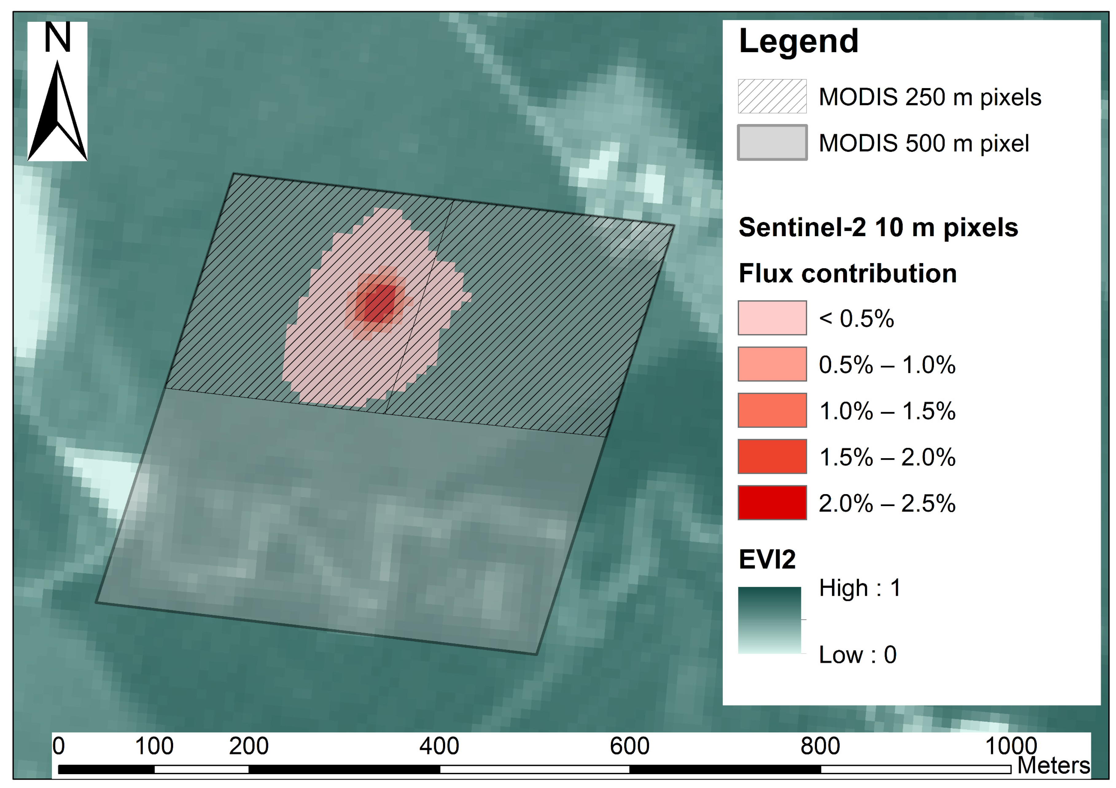
2.2. Eddy Covariance Influence Area

To estimate the approximation of the climatological footprint of the EC measurements, we used the Matlab implementation of the Flux Footprint Prediction (FFP) model of Kljun et al. [39], which provides position, size, and contribution details of surface source areas. Most of the input variables were collected as a part of the EC systems at the sites. The displacement height was defined as 0.67 times the canopy height. The boundary layer height was not measured directly at the sites but estimated using the friction velocity, Obukhov length and latitude of the site for near-neutral and stable conditions following Kljun et al. [39]. For convective conditions the boundary layer was set to be 1500 m.

Through input half-hourly measured data (meeting the condition that the friction velocity was higher than 0.1 m s⁻¹) to the FFP model, we obtained annual flux footprint climatology contours (Figure 2) and contribution weights in 10 m resolution pixel (matched to Sentinel-2 pixel). Following the suggestion in Kljun et al. [39], we used the 80% flux footprint contribution contour line as the maximum footprint area since it is sufficient for estimating the main source area in most cases.

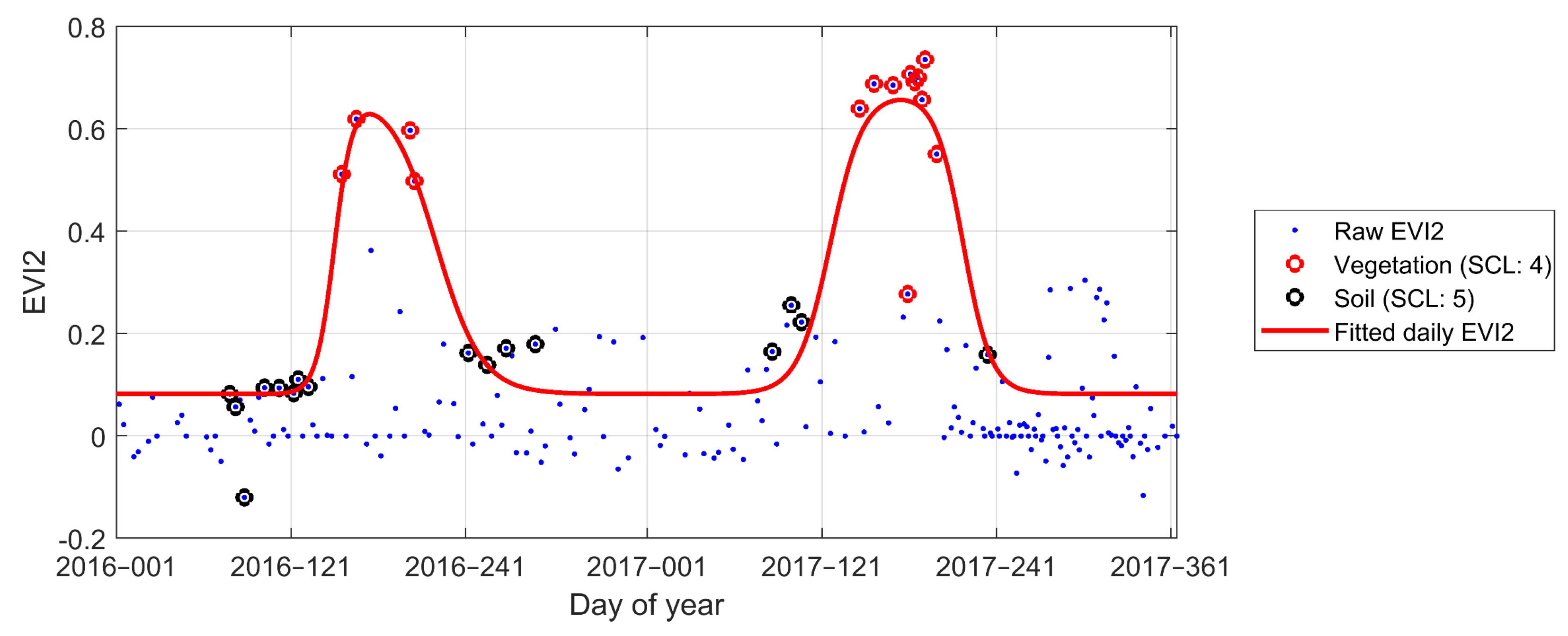
2.3. Daily EVI2 Trajectories of Satellite Pixels

The eight ICOS sites are covered by seven Sentinel-2 MSI tiles. A total of 1312 available Sentinel-2 images acquired in 2016 and 2017 for the seven tiles were downloaded from the ESA Copernicus Sentinels Scientific Data Hub [57]. The Sen2Cor processor (version 2.5.5) was applied for atmospheric correction to obtain Level-2A surface reflectance and scene classification layer (SCL) [58]. EVI2 of each Sentinel-2 pixel (10m resolution) was calculated by red reflectance ($\rho RED$) and near-infrared reflectance ($\rho NIR$) using the following equation:

$$EVI2=2.5\times \frac{\rho NIR-\rho RED}{\rho NIR+ 2.4\times \rho RED+1} .$$

(1)

Through the SCL, pixels recorded as vegetation and soil were marked as high quality, whereas those recorded as cloud, snow, and water, were marked as low quality. Two different spatial resolution MODIS EVI2 (250 m and 500 m) datasets for 2016 and 2017 were generated from MODIS/Terra MOD09Q1 (250 m) and MOD09A1 (500 m) [59] to be comparable to Sentinel-2 EVI2. Each MODIS pixel’s quality flag was created from the binary MODIS quality (QA) data.

For generating daily EVI2 time-series from Sentinel-2 data and MODIS data, we applied a time-series fitting algorithm, box constrained separable least squares fitting to double logistic model functions [60], so that the datasets could be compared. This is a time-series fitting method that reduces noise, gap-fills the data, and generates output a regular time step (Figure 3). The inputs of the method were EVI2 time-series and quality flags. Only highest quality data were used in the function fitting. To avoid errors due to unequal time sampling of MODIS [61], the actual acquisition dates of the MODIS observations were used as a time vector of the MODIS EVI2 time-series. The default procedure and settings as described by Jönsson et al. [60] were applied to produce daily EVI2 time-series. The fitting method is similar to the commonly used double logistic model functions [62] but with the following three differences: (1) the box constrained method applies a constant base level, which was estimated from a 5% low threshold of the clear observation histogram for the full time-series; (2) through a shape prior, i.e., a common season estimated for the full time-series through which the box constrained method improves the reconstruction of the seasons also in cases when the amount of observation data is insufficient; and (3) where the observation data was sufficiently large over a growing season, the estimation of parameters of the double logistic function for the season was constrained within a set of ranges (‘box’) in the box constrained method.

2.4. Daily EVI2 of Flux Footprint

The pixels’ daily EVI2 trajectories, which were generated from the previous section, were further used to estimate daily EVI2 over the flux footprint. To compute MODIS 250 m EVI2 averages over the flux footprint area, denoted as EVI2_250m, a maximum of four pixels around the tower were used, and 500 m EVI2 averages (EVI2_500m) were computed from the 500 m pixel(s) where the towers are located (Figure 4). Sentinel-2 weighted averages over the flux footprint areas, denoted as EVI2_10m, were thus computed from 450–5800 pixels depending on the estimated footprint size. Since 10 m Sentinel-2 pixels are much smaller than flux footprints, we calculated the footprint EVI2 more precisely by

$$EVI{2}_{10m}={{\displaystyle \sum }}_{i=1}^{n}EVI{2}_i\ast w_i ,$$

(2)

where $EVI{2}_{10m}$ is the footprint EVI2; $n$ is the number of Sentinel-2 pixels covering the flux footprint; $EVI{2}_i$ and $w_i$ (0–1) are EVI2 of the pixel $i$ and the corresponding contribution weight to the total flux.

2.5. Empirical Regression Models for GPP Estimation

For the eight stations, regression models were used to estimate daily GPP (g C m⁻² day⁻¹) following previously tested model formulations for our study region by Schubert et al. [27], one model for each ICOS site:

$$GPP=a\times EVI2\times E+b,$$

(3)

where the variable $EVI2$ is daily averaged EVI2 reconstructed by the box constrained method from Sentinel-2 MSI data and MODIS data. $E$ is the EC tower measured daily sum of PPFD (µmol m⁻² day⁻¹), the daily average air temperature T_a (°C), the daily average VPD (hPa) or the product of them. Available light and temperatures above the freezing point are requirements for photosynthesis. Therefore, only dates with both a daily sum PPFD larger than 0 µmol m⁻² day⁻¹ and a daily average T_a above 0 °C were used in the further model calculation. $E$ in the model was smoothed by a moving average with a 7-day moving window for reducing the noise of the data. Although there would be six possible model formulas based on the combinations between satellite-derived EVI2 and the different environmental variables at each site, a single model formula was required to enable a direct comparison between Sentinel-2 MSI EVI2 and MODIS EVI2 at each site. The selection of this single model formula was achieved by assessing the coefficient of determination values (R²) and root mean square error (RMSE) between the EC GPP and model estimated GPP.

To evaluate the EVI2-driven GPP models, we computed the root mean square error (RMSE), mean absolute error (MAE) and R² between EVI2-driven daily GPP ($GP{P}_{EVI2}$) and EC-driven daily GPP ($GP{P}_{EC}$) for each GPP site:

$$RMSE= \sqrt{\frac{{{\displaystyle \sum }}_{i=1}^n{(GP{P}_{EVI2}-GP{P}_{EC})}^2}{n}},$$

(4)

$$MAE= \frac{{{\displaystyle \sum }}_{i=1}^n\left|GP{P}_{EVI2}-GP{P}_{EC}\right|}{n},$$

(5)

where $n$ is the number of valid days for modelling GPP at the site.

In order to further clarify whether the RMSE, MAE, and R² at different spatial resolutions (10 m, 250 m and 500 m) are significantly different, we used the Wilcoxon signed-rank test to perform pairwise tests with a null hypothesis of zero medians for the difference of RMSE/MAE/R² between paired sample sites.

3. Results

3.1. Relationships between GPP, EVI2 and Environmental Variables

Daily EVI2 from Sentinel-2 MSI and MODIS all showed linear relationships with flux tower-derived GPP (R² = 0.45–0.93,

Table 2. Coefficient of determination, R², of environmental variables/satellite EVI2 versus EC derived GPP in daily time step. No VPD data were available at FI-Hyy site.

	EVI210m	EVI2250m	EVI2500m	Ta	PPFD	VPD
SE-Sto	0.77	0.81	0.83	0.69	0.04	0.24
SE-Svb	0.74	0.73	0.79	0.86	0.51	0.41
SE-Deg	0.59	0.58	0.63	0.68	0.28	0.34
FI-Hyy	0.73	0.83	0.86	0.87	0.54	-
SE-Nor	0.81	0.67	0.72	0.82	0.74	0.53
SE-Lnn	0.89	0.93	0.90	0.31	0.49	0.23
SE-Htm	0.78	0.45	0.56	0.75	0.82	0.43
DK-Sor	0.93	0.87	0.89	0.79	0.76	0.57

). There was no tendency for stronger relationships with higher resolution data. MODIS EVI2 showed stronger relationships than Sentinel-2 at four sites; however, at the evergreen forest site SE-Htm, the relationships with EC GPP were considerably weaker than for Sentinel-2 (R² = 0.45 and 0.56). Comparing the two MODIS resolutions, the higher spatial resolution EVI2_250m provided stronger relationships with flux tower GPP at the agricultural site SE-Lnn. At this site and the deciduous forest site DK-Sor, daily EVI2 at all spatial resolutions from both Sentinel-2 MSI and MODIS showed very strong relationships with flux tower GPP (R² > 0.85).

The environmental variables showed lower correlations with GPP than EVI2 for five of the eight sites. T_a had higher R² than PPFD at most sites, expect at the agricultural site SE-Lnn and the evergreen forest site SE-Htm. For PPFD, R² values were lower at high latitudes than at low latitudes, and values at the forest sites were higher than values for the agricultural and wetland sites. VPD showed the weakest relationships among all three environmental variables at all sites. In DK-Sor and SE-Nor, however, the relationships between VPD and GPP were relatively strong, with R² values of 0.57 and 0.53, respectively. Spring 2017 was relatively dry in the study areas and for SE-Nor summer 2017 remained dry which increased the sensitivity to VPD. Otherwise, shallow soil depth at these sites might affect the water storage capacity. Despite this, the influence of VPD seemed to be low for most of the sites so only EVI2, T_a and PPFD were chosen for the final regression models, because of their stronger relationships with GPP.

3.2. Multiple Linear Regression Models of GPP

Based on the general relationships shown in Table 2, and with the aim of fitting models that had the same formulation for the three satellite data sets at each site, $T_a$ was chosen as input environmental variables into the final linear GPP regression model:

$$GPP=a\times EVI2\times T_a+b.$$

(6)

We tested three models at all sites, and the RMSEs, MAEs, and R² of satellite-derived GPP and flux data-derived GPP were calculated (

Table A1. RMSEs, MAEs, and R² between EC driven GPP (g C m⁻² day⁻¹) and EVI2 driven GPP from three linear models in 10 m, 250 m, and 500 m resolutions at eight Nordic sites. The three linear models are model I: $GPP=a·T_a·EVI2+b$, model II: $GPP=a·PPFD·EVI2+b$, and model III: $GPP=a·T_a·PPFD·EVI2+b$.

		Model I			Model II			Model III
	Resolution	RMSE	MAE	R2	RMSE	MAE	R2	RMSE	MAE	R2
SE-Sto	10 m	0.49	0.39	0.83	0.97	0.76	0.33	0.74	0.54	0.62
	250 m	0.45	0.35	0.86	0.95	0.73	0.37	0.73	0.54	0.62
	500 m	0.44	0.35	0.86	0.93	0.72	0.39	0.71	0.53	0.64
SE-Svb	10 m	1.12	0.95	0.87	1.83	1.57	0.67	1.50	1.20	0.77
	250 m	1.10	0.94	0.88	1.80	1.55	0.68	1.49	1.20	0.78
	500 m	1.04	0.88	0.89	1.76	1.52	0.69	1.48	1.20	0.78
SE-Deg	10 m	0.51	0.39	0.71	0.62	0.49	0.56	0.56	0.42	0.64
	250 m	0.52	0.40	0.69	0.65	0.52	0.52	0.58	0.44	0.61
	500 m	0.51	0.40	0.70	0.63	0.50	0.55	0.57	0.44	0.62
FI-Hyy	10 m	0.98	0.73	0.89	1.76	1.39	0.65	1.01	0.78	0.88
	250 m	0.96	0.71	0.89	1.38	1.09	0.78	0.92	0.72	0.90
	500 m	0.96	0.70	0.89	1.34	1.06	0.79	0.91	0.72	0.90
SE-Nor	10 m	1.27	1.02	0.84	1.36	0.97	0.81	1.21	0.95	0.85
	250 m	1.36	1.09	0.81	1.35	0.94	0.81	1.24	0.96	0.84
	500 m	1.33	1.07	0.82	1.27	0.89	0.84	1.24	0.99	0.84
SE-Lnn	10 m	1.60	1.03	0.88	1.50	0.90	0.90	1.73	1.08	0.86
	250 m	1.60	1.19	0.88	1.33	1.02	0.92	1.47	0.98	0.90
	500 m	1.96	1.43	0.82	1.56	1.14	0.89	1.77	1.19	0.85
SE-Htm	10 m	1.92	1.63	0.77	1.49	1.09	0.86	1.85	1.50	0.79
	250 m	2.13	1.83	0.72	1.36	0.97	0.88	1.84	1.48	0.79
	500 m	2.09	1.81	0.73	1.29	0.93	0.90	1.81	1.46	0.79
DK-Sor	10 m	1.91	1.44	0.91	1.59	1.16	0.93	1.76	1.29	0.92
	250 m	2.19	1.68	0.88	1.95	1.37	0.90	1.79	1.28	0.92
	500 m	2.12	1.63	0.88	1.96	1.39	0.90	1.78	1.29	0.92
Average	10 m	0.49	0.39	0.83	0.97	0.76	0.33	0.74	0.54	0.62
	250 m	0.45	0.35	0.86	0.95	0.73	0.37	0.73	0.54	0.62
	500 m	0.44	0.35	0.86	0.93	0.72	0.39	0.71	0.53	0.64

Note: the numbers in bold type are the smallest RMSEs, the smallest MAEs, and the largest R² in the three models.

). We found that the differences of RMSE, MAE, and R² due to the differences in the model were greater than those due to the difference in the satellite data. Referring to the RMSEs from the three models at each site (Table A1), we used the model that generated the highest R² at each site for the final GPP estimation results (

Table 3. Linear regressions for GPP (g C m⁻² day⁻¹) at each site driven by the products of T_a and EVI2 in 10 m from Sentinel-2, and 250 m, 500 m from MODIS.

	Resolution	$\mathit{a}$	$\mathit{b}$	RMSE 1	MAE 1	R2
SE-Sto	10 m	0.61	−0.23	0.49	0.39	0.83
	250 m	0.60	−0.17	0.45	0.35	0.86
	500 m	0.69	−0.13	0.44	0.35	0.86
SE-Svb	10 m	1.72	1.06	1.12	0.95	0.87
	250 m	1.77	1.09	1.10	0.94	0.88
	500 m	1.71	1.20	1.04	0.88	0.89
SE-Deg	10 m	0.54	0.10	0.51	0.39	0.71
	250 m	0.42	0.13	0.52	0.40	0.69
	500 m	0.42	0.12	0.51	0.40	0.70
FI-Hyy	10 m	1.34	0.61	0.98	0.73	0.89
	250 m	1.17	0.78	0.96	0.71	0.89
	500 m	1.13	0.87	0.96	0.70	0.89
SE-Nor	10 m	1.28	0.63	1.27	1.02	0.84
	250 m	1.29	0.68	1.36	1.09	0.81
	500 m	1.20	0.81	1.33	1.07	0.82
SE-Lnn	10 m	1.25	−0.18	1.60	1.03	0.88
	250 m	1.23	−0.68	1.60	1.19	0.88
	500 m	1.23	−0.71	1.96	1.43	0.82
SE-Htm	10 m	1.56	1.00	1.92	1.63	0.77
	250 m	1.39	1.24	2.13	1.83	0.72
	500 m	1.25	1.50	2.09	1.81	0.73
DK-Sor	10 m	1.35	−0.36	1.91	1.44	0.91
	250 m	1.52	−0.81	2.19	1.68	0.88
	500 m	1.54	−0.84	2.12	1.63	0.88

¹ in unit g C m⁻² d⁻¹.

). Therefore, we applied the model driven by $T_a$ (Equation (5)) at all sites.

The slopes and intercepts of the regression models are similar within the same site (Table 3). The largest differences of slopes and intercepts among the different satellite EVI2 data were found at the three southern sites, SE-Lnn, SE-Htm, and DK-Sor. RMSEs, MAEs, and R² had similar patterns across sites, satellite data sets and model formulations, which means that the low RMSE values usually coincided with low MAE and high R² values. There was no single satellite dataset that always generated the lowest RMSE, lowest MAE, or highest R². RMSE, as well as MAE and R², differed mostly across sites, and the smallest differences were found between the EVI2 variables from the different satellite datasets (Table A1). All the p-values shown in

Table 4. Paired p-values of RMSE, MAE and R² over 8 sites from Wilcoxon signed-rank test. All p-values of 0.10 over fail to reject the null hypothesis.

RMSE			MAE			R2
	250 m	500 m		250 m	500 m		250 m	500 m
10 m	0.547	0.313	10 m	0.250	0.313	10 m	0.461	0.461
500 m	0.195	-	500 m	0.250	-	500 m	0.195	-

from Wilcoxon signed-rank tests are over 0.10, which means that the test failed to reject the null hypothesis of zero medians for the difference of RMSE/MAE/R² between paired sample sites. Separately averaging RMSE, MAE, and R² across sites, it was seen that there was almost no difference in the results generated from Sentinel-2 MSI data and MODIS data (

Table 5. Average errors and coefficients of determination across sites.

Resolution	RMSE 1	MAE 1	R2
10 m	1.23	0.95	0.84
250 m	1.29	1.02	0.83
500 m	1.31	1.03	0.82

¹ in unit g C m⁻² d⁻¹.

).

The modelled GPP time-series were very close between Sentinel-2 and 250 m MODIS data at all sites (Figure 5). The shape and magnitude of the daily GPP time-series between satellite driven GPP and flux data-derived GPP were similar (Figure 5). Peak season GPP decreased from the south to the north. The subarctic and boreal mire sites (SE-Sto and SE-Deg, respectively) had much smaller peak GPP (less than 5 g C m⁻² d⁻¹) compared to other sites. The GPP peak at the coniferous forest sites varied between 10–15 g C m⁻² d⁻¹, whereas the deciduous and agricultural sites had the peak around 15–20 g Cm⁻² d⁻¹. The agriculture site SE-Lnn had high peak GPP but a relatively short growing season with a narrow shape, mainly controlled by the activities of cultivation. The GPP time-series pattern at the deciduous and evergreen forest sites, DK-Sor and SE-Htm, was much wider than at SE-Lnn, which indicates a much longer growing season (Figure 5).

4. Discussion

The results showed that for all sites and all satellite products, the relationship between EVI2 and the flux tower modelled GPP was generally strong (Table 2). This means that seasonal GPP variations can be estimated at different resolutions, from 500 down to 10 m spatial resolution, implying that remotely sensed data has the potential to provide highly detailed spatial estimates of carbon uptake dynamics across northern boreal landscapes. This tool can contribute to future work on carbon-friendly forest management and climate mitigation.

The model selection using climatological flux footprint led to a linear regression model, driven by T_a, in combination with satellite reconstructed daily EVI2 (Equation (6)). However, the selected model is not always optimal for each site (Table A1). The agricultural sites and deciduous forest sites had a larger seasonal variation of greening in comparison with the evergreen coniferous forest sites, which helps to explain the strong relationship between EVI2 and GPP in SE-Lnn and DK-Sor. Air temperature was the most important environmental variable for estimating GPP at the northern sites (SE-Sto, SE-Svb, SE-Deg and FI-Hyy) whereas at the southern sites (SE-Nor, SE-Lnn, SE-Htm and DK-Sor) the differences between models were small. This is explained by the fact that in the northern part of our study area the growing season begins when the temperature exceeds the temperature limit, which occurs well after the amount of light has reached sufficient levels for photosynthesis [63,64]. This finding indicates that, although EVI2 is the most important driving variable overall, choosing the correct model formulation is important for GPP estimation across a study area traversing such a large latitudinal range.

The method of estimating GPP used in this study is similar to the method proposed by Schubert et al. [27] regarding the methodology, model design and study area, but we used finer spatial and temporal resolution satellite data, dynamic flux footprint, and ground-based measured environmental variables. In comparison with the study by Schubert et al. [27], we used four common sites: SE-Sto, FI-Hyy, SE-Nor and DK-Sor. The estimation of GPP has small RMSE and higher R² at site SE-Sto, but it has larger RMSE and lower R² at site FI-Hyy. The RMSEs are larger but R² are lower at sites SE-Nor and DK-Sor. One of the reasons for this inconsistency is that we used a different time period in the study.

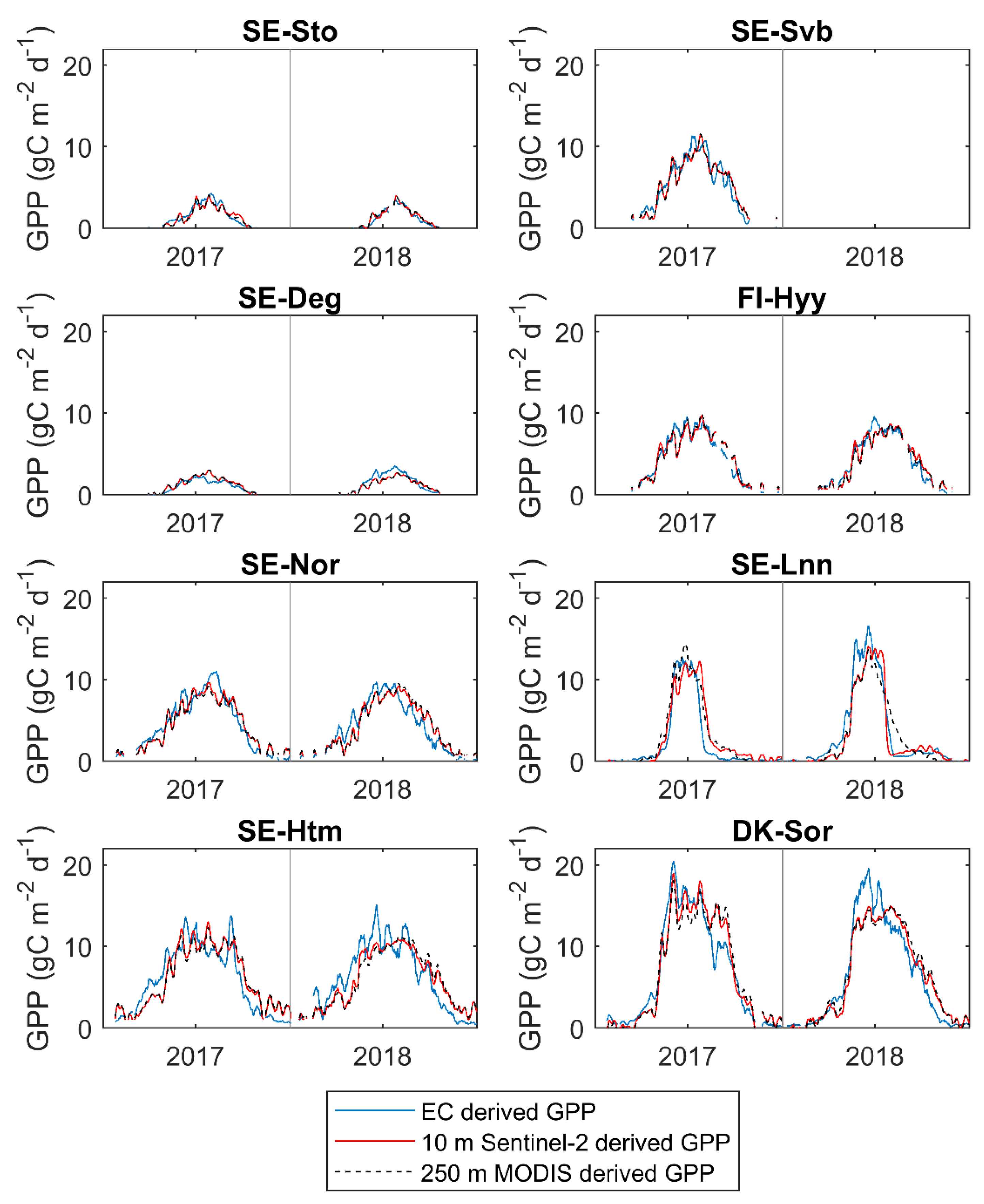
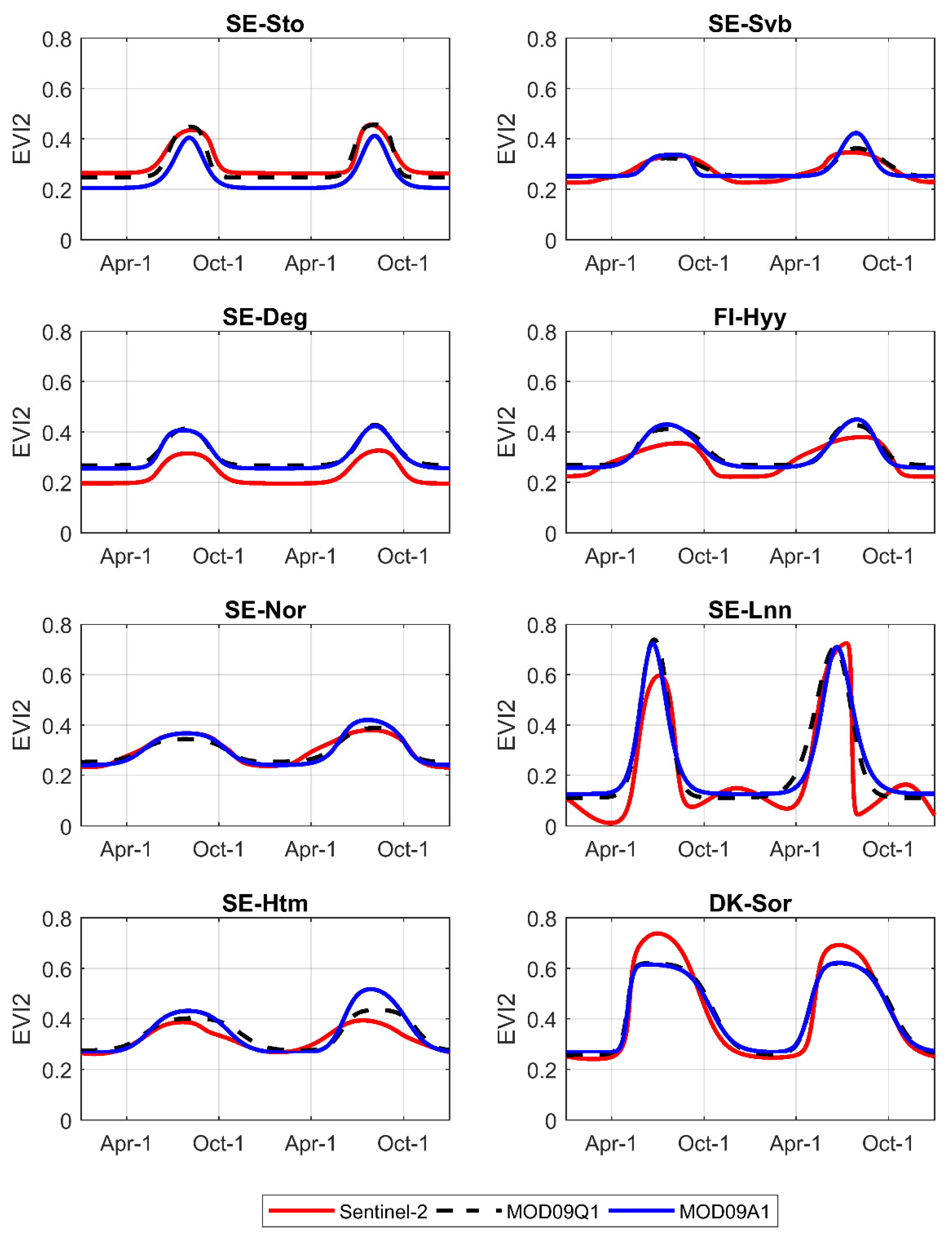
4.1. Similar Performance of Sentinel-2 and MODIS on GPP Modelling

Despite its finer spatial resolution, Sentinel-2 data did not enhance the performance of the empirical GPP models. This result is mainly explained by the homogeneous surrounding vegetation of the EC areas in combination with the quite large area of flux footprint; however, other factors that may have contributed to this result are, e.g., (1) the function fitting model used eliminated minor fluctuations of EVI2 time-series, which might have masked some differences among the input datasets; (2) the use of linear regression models reduced the magnitude difference between Sentinel-2 EVI2 and MODIS EVI2 data. These points are further discussed below.

A factor that strongly reduced the differences in GPP relationships between Sentinel-2 and MODIS was the homogeneity of the EC sites. We applied the FFP model to more precisely estimate the EC measurements’ footprint [35,39]. The coverage areas of MODIS pixels and Sentinel-2 pixels that are used to represent the flux footprint are quite different at some sites, e.g., SE-Lnn. However, the footprint EVI2 in Sentinel-2 and MODIS scales did not show large differences due to the homogeneity of the surrounding areas of EC measurement.

As previously mentioned, the satellite daily EVI2 time-series were generated based on double logistic functions, which are robust at handling data gaps and reducing data noise but lead to a loss of daily fluctuations of the EVI2. Therefore, the day-by-day fluctuations in the output GPP were all mainly generated by T_a or PPFD. Since the same environmental datasets were applied to the GPP models for all satellite data, the differences in the GPP outputs between the satellite datasets at each site only reflect the differences in fitted EVI2. Thus, the seasonal shape and magnitude of EVI2 make up the principal differences between the GPP of the different satellite datasets (Figure A1 in Appendix A). Our previous experiences show that Sentinel-2 MSI EVI2 time-series perform better than MODIS in capturing ground multispectral measured EVI2 time-series [65]. However, in the current study, the effects of the differences in seasonal shape and magnitude of EVI2 time-series on GPP modelling at each site were reduced by the intercepts ($a$) and slopes ($b$) in the linear regression models. The intercepts reduced the bias of estimations, while the slopes reduced the differences in the amplitudes of the estimations.

In a recently published study, Wang et al. [11] applied a very high resolution (VHR) hyperspectral sensor on a UAV platform, to study the effects of spatial resolution on the model performance in a willow field at a 30 minutes’ flux basis. They found that the performance of footprint weighted simulations to represent the measured flux started to decline as resolutions exceeded 10 m, while performance was high and relatively constant from 0.03 m to 10 m. They compared their results with the typical scales of the canopy structure and concluded that the spatial resolution should be in the same order of magnitude as the typical crown sizes and distances between the plant rows. While this high requirement might be typical for a homogeneous study site as the willow plantation, the rule of thumb might be general [11]. Yet the spatial resolutions of satellite-based remote sensing techniques are currently much coarser.

4.2. Challenges and Outlook

In this study, we did not separate the data into training data and evaluation data. This was because of the limited number of flux sites and the short coverage time of Sentinel-2 in Northern Europe, and because our main concern was the ability of Sentinel-2 and MODIS to drive the GPP models but not the absolute accuracy of the prediction model. With more data in the future, it will be possible to fine-tune an accurate model by dividing the data into training data and evaluation data. The high p-values in the test indicated that the conclusion of no significant differences between the data sets may change with a larger sample size.

Although the empirical regression models were generally accurate, further GPP model development may need to be carried out when developing upscaling methodology from Sentinel-2 MSI. The fact that model selection had more impact on the accuracies than the choice of input data highlights the importance of further studying the input environmental drivers and the model formulations for estimating GPP, e.g., Tagesson et al. [66]. To further improve the match between flux tower EC data and remote sensing, applying daily rather than annual footprint climatologies is a possibility that should be pursued in future studies [38,39]. This is a rather complex analysis and given the small differences observed between the different data sets it is not likely that this would radically change the conclusions in the current study. For upscaling across large areas, a practically applicable methodology needs to be developed (such as the abovementioned study by Wang et al. [11]). It may also be fruitful to further investigate the drivers behind the spatial variation of GPP, e.g., canopy openness or leaf area index, and find suitable remote sensing variables that directly or indirectly represent these drivers. Another factor to consider is the contribution of the understory vegetation to the ecosystem carbon exchange, which is not usually taken into account in satellite-derived GPP models. This affects remotely sensed data [67] and could account for errors in GPP estimates at the beginning and the end of the growing season [68]. Along with EC towers, flux chambers may be useful for mapping spatial heterogeneity in GPP in low vegetation areas [69].

With regard to satellite data processing, we suggest analyzing more efficient vegetation indices, e.g., the Plant Phenology Index, which has shown to correlate more strongly with GPP than EVI or NDVI [70,71]. Though efficient, this index requires angular effects to be corrected for, which precluded us from using the index with the available Sentinel-2 data.

5. Conclusions

In this paper, we examined the effect of the spatial resolution of daily two-band enhanced vegetation index (EVI2, 10m from Sentinel-2 MSI, 250m and 500m from MODIS) on the accuracy of gross primary productivity (GPP) estimations with different regression models at eight Nordic eddy covariance flux sites. The results gave high and consistent coefficients of explanation (R² = 0.84 for Sentinel-2; R² = 0.83 for MODIS) verifying the potential of remotely sensed data to provide accurate estimates of the seasonal carbon uptake dynamics across northern boreal landscapes at both the coarse and fine spatial scale. Sentinel-2 opens the possibility of very detailed GPP estimation across the northern landscape, which is of benefit for climate mitigation and adaptation work. The analysis showed that the quantitative differences in GPP estimation due to the different input data were small between Sentinel-2 MSI GPP and MODIS GPP; smaller than the effect of different model formulations. This can be explained by the combined effects of the higher temporal frequency of MODIS compensating for its lower spatial resolution, the time-series fitting method used for reconstructing daily EVI2, the homogeneity of the surrounding areas of the EC measurements, and the use of linear regression models. To further strengthen the development of GPP models based on Sentinel-2 data will require more analyses of different model formulations (including environmental drivers), more tests of remotely sensed indices and biophysical parameters, and analyses across a wider range of geographical locations and time.

References

1. Pachauri, R.K.; Allen, M.R.; Barros, V.R.; Broome, J.; Cramer, W.; Christ, R.; Church, J.A.; Clarke, L.; Dahe, Q.; Dasgupta, P. Climate Change 2014: Synthesis Report. Contribution of Working Groups I, II and III to the Fifth Assessment Report of the Intergovernmental Panel on Climate Change; IPCC: Geneva, Switzerland, 2014. [Google Scholar]
2. Jung, M.; Reichstein, M.; Margolis, H.A.; Cescatti, A.; Richardson, A.D.; Arain, M.A.; Arneth, A.; Bernhofer, C.; Bonal, D.; Chen, J. Global patterns of land-atmosphere fluxes of carbon dioxide, latent heat, and sensible heat derived from eddy covariance, satellite, and meteorological observations. J. Geophys. Res. Biogeosci. 2011, 116. [Google Scholar] [CrossRef] [Green Version]
3. Pan, Y.; Birdsey, R.A.; Fang, J.; Houghton, R.; Kauppi, P.E.; Kurz, W.A.; Phillips, O.L.; Shvidenko, A.; Lewis, S.L.; Canadell, J.G.; et al. A large and persistent carbon sink in the world’s forests. Science 2011, 333, 988–993. [Google Scholar] [CrossRef] [Green Version]
4. Graven, H.D.; Keeling, R.F.; Piper, S.C.; Patra, P.K.; Stephens, B.B.; Wofsy, S.C.; Welp, L.R.; Sweeney, C.; Tans, P.P.; Kelley, J.J.; et al. Enhanced seasonal exchange of CO2 by northern ecosystems since 1960. Science 2013, 341, 1085–1089. [Google Scholar] [CrossRef] [PubMed] [Green Version]
5. Baldocchi, D.D. Assessing the eddy covariance technique for evaluating carbon dioxide exchange rates of ecosystems: Past, present and future. Glob. Chang. Biol. 2003, 9, 479–492. [Google Scholar]
6. Lagergren, F.; Grelle, A.; Lankreijer, H.; Mölder, M.; Lindroth, A. Current carbon balance of the forested area in sweden and its sensitivity to global change as simulated by Biome-BGC. Ecosystems 2006, 9, 894–908. [Google Scholar] [CrossRef]
7. Monteith, J.L. Solar radiation and productivity in tropical ecosystems. J. Appl. Ecol. 1972, 9, 747–766. [Google Scholar] [CrossRef] [Green Version]
8. Goetz, S.J.; Prince, S.D.; Goward, S.N.; Thawley, M.M.; Small, J. Satellite remote sensing of primary production: An improved production efficiency modeling approach. Ecol. Model. 1999, 122, 239–255. [Google Scholar] [CrossRef]
9. Sasai, T.; Okamoto, K.; Hiyama, T.; Yamaguchi, Y. Comparing terrestrial carbon fluxes from the scale of a flux tower to the global scale. Ecol. Model. 2007, 208, 135–144. [Google Scholar] [CrossRef]
10. Zhou, Y.; Wu, X.; Ju, W.; Chen, J.M.; Wang, S.; Wang, H.; Yuan, W.; Andrew Black, T.; Jassal, R.; Ibrom, A. Global parameterization and validation of a two-leaf light use efficiency model for predicting gross primary production across FLUXNET sites. J. Geophys. Res. Biogeosci. 2016, 121, 1045–1072. [Google Scholar] [CrossRef]
11. Wang, S.; Garcia, M.; Bauer-Gottwein, P.; Jakobsen, J.; Zarco-Tejada, P.J.; Bandini, F.; Paz, V.S.; Ibrom, A. High spatial resolution monitoring land surface energy, water and CO2 fluxes from an Unmanned Aerial System. Remote. Sens. Environ. 2019, 229, 14–31. [Google Scholar] [CrossRef]
12. Ibrom, A.; Oltchev, A.; June, T.; Kreilein, H.; Rakkibu, G.; Ross, T.; Panferov, O.; Gravenhorst, G. Variation in photosynthetic light-use efficiency in a mountainous tropical rain forest in Indonesia. Tree Physiol. 2008, 28, 499–508. [Google Scholar] [CrossRef] [PubMed] [Green Version]
13. Propastin, P.; Ibrom, A.; Knohl, A.; Erasmi, S. Effects of canopy photosynthesis saturation on the estimation of gross primary productivity from MODIS data in a tropical forest. Remote Sens. Environ. 2012, 121, 252–260. [Google Scholar] [CrossRef]
14. Medlyn, B.E. Physiological basis of the light use efficiency model. Tree Physiol. 1998, 18, 167–176. [Google Scholar] [CrossRef] [PubMed]
15. Turner, D.P.; Urbanski, S.; Bremer, D.; Wofsy, S.C.; Meyers, T.; Gower, S.T.; Gregory, M. A cross-biome comparison of daily light use efficiency for gross primary production. Glob. Chang. Biol. 2003, 9, 383–395. [Google Scholar] [CrossRef]
16. Ibrom, A.; Jarvis, P.G.; Clement, R.; Morgenstern, K.; Oltchev, A.; Medlyn, B.E.; Wang, Y.P.; Wingate, L.; Moncrieff, J.B.; Gravenhorst, G. A comparative analysis of simulated and observed photosynthetic CO2 uptake in two coniferous forest canopies. Tree Physiol. 2006, 26, 845–864. [Google Scholar] [CrossRef] [Green Version]
17. Fensholt, R.; Sandholt, I.; Rasmussen, M.S. Evaluation of MODIS LAI, fAPAR and the relation between fAPAR and NDVI in a semi-arid environment using in situ measurements. Remote Sens. Environ. 2004, 91, 490–507. [Google Scholar] [CrossRef]
18. Glenn, E.; Huete, A.; Nagler, P.; Nelson, S. Relationship between remotely-sensed vegetation indices, canopy attributes and plant physiological processes: What vegetation indices can and cannot tell us about the landscape. Sensors 2008, 8, 2136. [Google Scholar] [CrossRef] [Green Version]
19. Hilker, T.; Coops, N.C.; Wulder, M.A.; Black, T.A.; Guy, R.D. The use of remote sensing in light use efficiency based models of gross primary production: A review of current status and future requirements. Sci. Total Environ. 2008, 404, 411–423. [Google Scholar] [CrossRef] [Green Version]
20. Huete, A.; Didan, K.; Miura, T.; Rodriguez, E.P.; Gao, X.; Ferreira, L.G. Overview of the radiometric and biophysical performance of the MODIS vegetation indices. Remote Sens. Environ. 2002, 83, 195–213. [Google Scholar] [CrossRef]
21. Running, S.W.; Nemani, R.R.; Heinsch, F.A.; Zhao, M.; Reeves, M.; Hashimoto, H. A Continuous Satellite-Derived Measure of Global Terrestrial Primary Production. BioScience 2004, 54, 547–560. [Google Scholar] [CrossRef]
22. Wu, C.; Chen, J.M.; Desai, A.R.; Hollinger, D.Y.; Arain, M.A.; Margolis, H.A.; Gough, C.M.; Staebler, R.M. Remote sensing of canopy light use efficiency in temperate and boreal forests of North America using MODIS imagery. Remote Sens. Environ. 2012, 118, 60–72. [Google Scholar] [CrossRef]
23. Wang, S.; Ibrom, A.; Bauer-Gottwein, P.; Garcia, M. Incorporating diffuse radiation into a light use efficiency and evapotranspiration model: An 11-year study in a high latitude deciduous forest. Agric. For. Meteorol. 2018, 248, 479–493. [Google Scholar] [CrossRef] [Green Version]
24. Sims, D.A.; Rahman, A.F.; Cordova, V.D.; El-Masri, B.Z.; Baldocchi, D.D.; Flanagan, L.B.; Goldstein, A.H.; Hollinger, D.Y.; Misson, L.; Monson, R.K.; et al. On the use of MODIS EVI to assess gross primary productivity of North American ecosystems. J. Geophys. Res. Space Phys. 2006, 111. [Google Scholar] [CrossRef] [Green Version]
25. Olofsson, P.; Lagergren, F.; Lindroth, A.; Lindström, J.; Klemedtsson, L.; Kutsch, W.; Eklundh, L. Towards operational remote sensing of forest carbon balance across Northern Europe. Biogeosciences 2008, 5, 817–832. [Google Scholar] [CrossRef] [Green Version]
26. Sjöström, M.; Ardö, J.; Arneth, A.; Boulain, N.; Cappelaere, B.; Eklundh, L.; de Grandcourt, A.; Kutsch, W.L.; Merbold, L.; Nouvellon, Y.; et al. Exploring the potential of MODIS EVI for modeling gross primary production across African ecosystems. Remote Sens. Environ. 2011, 115, 1081–1089. [Google Scholar] [CrossRef]
27. Schubert, P.; Lagergren, F.; Aurela, M.; Christensen, T.; Grelle, A.; Heliasz, M.; Klemedtsson, L.; Lindroth, A.; Pilegaard, K.; Vesala, T.; et al. Modeling GPP in the Nordic forest landscape with MODIS time series data—Comparison with the MODIS GPP product. Remote Sens. Environ. 2012, 126, 136–147. [Google Scholar] [CrossRef]
28. Tucker, C.J. Red and photographic infrared linear combinations for monitoring vegetation. Remote Sens. Environ. 1979, 8, 127–150. [Google Scholar] [CrossRef] [Green Version]
29. Jiang, Z.; Huete, A.R.; Didan, K.; Miura, T. Development of a two-band enhanced vegetation index without a blue band. Remote Sens. Environ. 2008, 112, 3833–3845. [Google Scholar] [CrossRef]
30. Mäkelä, A.; Kolari, P.; Karimäki, J.; Nikinmaa, E.; Perämäki, M.; Hari, P. Modelling five years of weather-driven variation of GPP in a boreal forest. Agric. For. Meteorol. 2006, 139, 382–398. [Google Scholar] [CrossRef]
31. Zhao, M.; Running, S.W. Drought-Induced reduction in global terrestrial net primary production from 2000 through 2009. Science 2010, 329, 940–943. [Google Scholar] [CrossRef] [Green Version]
32. Weil, J.; Horst, T. Footprint estimates for atmospheric flux measurements in the convective boundary layer. In Precipitation Scavenging and Atmosphere-Surface Exchange; CRC Press: Washington, DC, USA, 1992; Volume 2, pp. 717–728. [Google Scholar]
33. Arriga, N.; Rannik, Ü.; Aubinet, M.; Carrara, A.; Vesala, T.; Papale, D. Experimental validation of footprint models for eddy covariance CO2 flux measurements above grassland by means of natural and artificial tracers. Agric. For. Meteorol. 2017, 242, 75–84. [Google Scholar] [CrossRef]
34. Schmid, H. Experimental design for flux measurements: Matching scales of observations and fluxes. Agric. For. Meteorol. 1997, 87, 179–200. [Google Scholar] [CrossRef]
35. Vesala, T.; Kljun, N.; Rannik, Ü.; Rinne, J.; Sogachev, A.; Markkanen, T.; Sabelfeld, K.; Foken, T.; Leclerc, M.Y. Flux and concentration footprint modelling: State of the art. Environ. Pollut. 2008, 152, 653–666. [Google Scholar] [CrossRef] [PubMed]
36. Wu, J.; Larsen, K.S.; van der Linden, L.; Beier, C.; Pilegaard, K.; Ibrom, A. Synthesis on the carbon budget and cycling in a Danish, temperate deciduous forest. Agric. For. Meteorol. 2013, 181, 94–107. [Google Scholar] [CrossRef]
37. Griebel, A.; Bennett, L.T.; Metzen, D.; Cleverly, J.; Burba, G.; Arndt, S.K. Effects of inhomogeneities within the flux footprint on the interpretation of seasonal, annual, and interannual ecosystem carbon exchange. Agric. For. Meteorol. 2016, 221, 50–60. [Google Scholar] [CrossRef]
38. Gelybó, G.; Barcza, Z.; Kern, A.; Kljun, N. Effect of spatial heterogeneity on the validation of remote sensing based GPP estimations. Agric. For. Meteorol. 2013, 174, 43–53. [Google Scholar] [CrossRef]
39. Kljun, N.; Calanca, P.; Rotach, M.W.; Schmid, H.P. A simple two-dimensional parameterisation for Flux Footprint Prediction (FFP). Geosci. Model Dev. 2015, 8, 3695–3713. [Google Scholar] [CrossRef] [Green Version]
40. Zhao, M.; Heinsch, F.A.; Nemani, R.R.; Running, S.W. Improvements of the MODIS terrestrial gross and net primary production global data set. Remote Sens. Environ. 2005, 95, 164–176. [Google Scholar] [CrossRef]
41. Turner, D.P.; Ritts, W.D.; Cohen, W.B.; Gower, S.T.; Running, S.W.; Zhao, M.; Costa, M.H.; Kirschbaum, A.A.; Ham, J.M.; Saleska, S.R.; et al. Evaluation of MODIS NPP and GPP products across multiple biomes. Remote Sens. Environ. 2006, 102, 282–292. [Google Scholar] [CrossRef]
42. Wang, X.; Ma, M.; Li, X.; Song, Y.; Tan, J.; Huang, G.; Zhang, Z.; Zhao, T.; Feng, J.; Ma, Z.; et al. Validation of MODIS-GPP product at 10 flux sites in northern China. Int. J. Remote Sens. 2013, 34, 587–599. [Google Scholar] [CrossRef]
43. Balzarolo, M.; Peñuelas, J.; Veroustraete, F. Influence of landscape heterogeneity and spatial resolution in multi-temporal in situ and MODIS NDVI data proxies for seasonal GPP dynamics. Remote Sens. 2019, 11, 1656. [Google Scholar] [CrossRef] [Green Version]
44. Lin, S.; Li, J.; Liu, Q.; Li, L.; Zhao, J.; Yu, W. Evaluating the Effectiveness of using vegetation indices based on red-edge reflectance from sentinel-2 to estimate gross primary productivity. Remote Sens. 2019, 11, 1303. [Google Scholar] [CrossRef] [Green Version]
45. Wolanin, A.; Camps-Valls, G.; Gómez-Chova, L.; Mateo-García, G.; van der Tol, C.; Zhang, Y.; Guanter, L. Estimating crop primary productivity with Sentinel-2 and Landsat 8 using machine learning methods trained with radiative transfer simulations. Remote Sens. Environ. 2019, 225, 441–457. [Google Scholar] [CrossRef]
46. Vrieling, A.; Meroni, M.; Darvishzadeh, R.; Skidmore, A.K.; Wang, T.; Zurita-Milla, R.; Oosterbeek, K.; O’Connor, B.; Paganini, M. Vegetation phenology from Sentinel-2 and field cameras for a Dutch barrier island. Remote Sens. Environ. 2018, 215, 517–529. [Google Scholar] [CrossRef]
47. Lange, M.; Dechant, B.; Rebmann, C.; Vohland, M.; Cuntz, M.; Doktor, D. Validating MODIS and Sentinel-2 NDVI products at a temperate deciduous forest site using two independent ground-based sensors. Sensors 2017, 17, 1855. [Google Scholar] [CrossRef] [PubMed] [Green Version]
48. Korhonen, L.; Hadi; Packalen, P.; Rautiainen, M. Comparison of Sentinel-2 and Landsat 8 in the estimation of boreal forest canopy cover and leaf area index. Remote Sens. Environ. 2017, 195, 259–274. [Google Scholar] [CrossRef]
49. Clevers, J.G.; Kooistra, L.; Van den Brande, M.M. Using Sentinel-2 data for retrieving LAI and leaf and canopy chlorophyll content of a potato crop. Remote Sens. 2017, 9, 405. [Google Scholar] [CrossRef] [Green Version]
50. Franz, D.; Acosta, M.; Altimir, N.; Arriga, N.; Arrouays, D.; Aubinet, M.; Aurela, M.; Ayres, E.; López-Ballesteros, A.; Barbaste, M.; et al. Towards long-term standardised carbon and greenhouse gas observations for monitoring Europe´s terrestrial ecosystems: A review. Int. Agrophys. 2018, 32, 439–455. [Google Scholar] [CrossRef]
51. Carrara, A.; Kolari, P.; Op de Beeck, M.; Berveiller, D.; Dengel, S.; Ibrom, A.; Merbold, L.; Rebmann, C.; Sabbatini, S.; Serrano-Ortiz, P. Radiation measurements at ICOS ecosystem stations. Int. Agrophys. 2018, 32, 589–605. [Google Scholar] [CrossRef]
52. De Beeck, M.O.; Gielen, B.; Merbold, L.; Ayres, E.; Serrano-Ortiz, P.; Acosta, M.; Pavelka, M.; Montagnani, L.; Nilsson, M.; Klemedtsson, L.; et al. Soil-meteorological measurements at ICOS monitoring stations in terrestrial ecosystems. Int. Agrophys. 2018, 32, 619–631. [Google Scholar] [CrossRef]
53. Rebmann, C.; Aubinet, M.; Schmid, H.; Arriga, N.; Aurela, M.; Burba, G.; Clement, R.; De Ligne, A.; Fratini, G.; Gielen, B.; et al. ICOS eddy covariance flux-station site setup: A review. Int. Agrophys. 2018, 32, 471–494. [Google Scholar] [CrossRef]
54. Sabbatini, S.; Mammarella, I.; Arriga, N.; Fratini, G.; Graf, A.; Hörtnagl, L.; Ibrom, A.; Longdoz, B.; Mauder, M.; Merbold, L.; et al. Eddy covariance raw data processing for CO2 and energy fluxes calculation at ICOS ecosystem stations. Int. Agrophys. 2018, 32, 495–515. [Google Scholar] [CrossRef]
55. Reichstein, M.; Falge, E.; Baldocchi, D.; Papale, D.; Aubinet, M.; Berbigier, P.; Bernhofer, C.; Buchmann, N.; Gilmanov, T.; Granier, A.; et al. On the separation of net ecosystem exchange into assimilation and ecosystem respiration: Review and improved algorithm. Glob. Chang. Biol. 2005, 11, 1424–1439. [Google Scholar] [CrossRef]
56. Wutzler, T.; Lucas-Moffat, A.; Migliavacca, M.; Knauer, J.; Sickel, K.; Šigut, L.; Menzer, O.; Reichstein, M. Basic and extensible post-processing of eddy covariance flux data with REddyProc. Biogeosciences 2018, 15, 5015–5030. [Google Scholar] [CrossRef] [Green Version]
57. Drusch, M.; Del Bello, U.; Carlier, S.; Colin, O.; Fernandez, V.; Gascon, F.; Hoersch, B.; Isola, C.; Laberinti, P.; Martimort, P.; et al. Sentinel-2: ESA’s Optical High-Resolution Mission for GMES Operational Services. Remote Sens. Environ. 2012, 120, 25–36. [Google Scholar] [CrossRef]
58. Louis, J.; Debaecker, V.; Pflug, B.; Main-Korn, M.; Bieniarz, J.; Mueller-Wilm, U.; Cadau, E.; Gascon, F. Sentinel-2 Sen2Cor: L2A Processor for Users. In Proceedings of the Living Planet Symposium, Milan, Italy, 13–17 May 2019; p. 91. [Google Scholar]
59. Vermote, E. MOD09Q1 MODIS/Terra Surface Reflectance 8-Day L3 Global 250m SIN Grid V006. NASA EOSDIS Land Process. DAAC 2015. [Google Scholar] [CrossRef]
60. Jönsson, P.; Cai, Z.; Melaas, E.; Friedl, M.; Eklundh, L. A Method for robust estimation of vegetation seasonality from landsat and Sentinel-2 time series Data. Remote Sens. 2018, 10, 635. [Google Scholar] [CrossRef] [Green Version]
61. Testa, S.; Mondino, E.C.B.; Pedroli, C. Correcting MODIS 16-day composite NDVI time-series with actual acquisition dates. Eur. J. Remote Sens. 2014, 47, 285–305. [Google Scholar] [CrossRef]
62. Fischer, A. A model for the seasonal variations of vegetation indices in coarse resolution data and its inversion to extract crop parameters. Remote Sens. Environ. 1994, 48, 220–230. [Google Scholar] [CrossRef]
63. Mäkelä, A.; Hari, P.; Berninger, F.; Hänninen, H.; Nikinmaa, E. Acclimation of photosynthetic capacity in Scots pine to the annual cycle of temperature. Tree Physiol. 2004, 24, 369–376. [Google Scholar] [CrossRef] [Green Version]
64. van Dijk, A.I.J.M.; Dolman, A.J.; Schulze, E.-D. Radiation, temperature, and leaf area explain ecosystem carbon fluxes in boreal and temperate European forests. Glob. Biogeochem. Cycles 2005, 19. [Google Scholar] [CrossRef]
65. Cai, Z. Vegetation Observation in the Big Data Era. Ph.D. Thesis, Lund University, Faculty of Science, Department of Physical Geography and Ecosystem Science, Lund, Sweden, 2019. [Google Scholar]
66. Tagesson, T.; Tian, F.; Schurgers, G.; Horion, S.; Scholes, R.; Ahlström, A.; Ardö, J.; Moreno, A.; Madani, N.; Olin, S. A physiology-based earth observation model indicate stagnation in the global gross primary production during recent decades. Glob. Chang. Biol. 2020, 27, 836–854. [Google Scholar] [CrossRef] [PubMed]
67. Eriksson, H.M.; Eklundh, L.; Kuusk, A.; Nilson, T. Impact of understory vegetation on forest canopy reflectance and remotely sensed LAI estimates. Remote Sens. Environ. 2006, 103, 408–418. [Google Scholar] [CrossRef]
68. Palmroth, S.; Bach, L.H.; Lindh, M.; Kolari, P.; Nordin, A.; Palmqvist, K. Nitrogen supply and other controls of carbon uptake of understory vegetation in a boreal Picea abies forest. Agric. For. Meteorol. 2019, 276–277, 107620. [Google Scholar] [CrossRef]
69. Schrier-Uijl, A.; Kroon, P.; Hensen, A.; Leffelaar, P.; Berendse, F.; Veenendaal, E. Comparison of chamber and eddy covariance-based CO2 and CH4 emission estimates in a heterogeneous grass ecosystem on peat. Agric. For. Meteorol. 2010, 150, 825–831. [Google Scholar] [CrossRef] [Green Version]
70. Karkauskaite, P.; Tagesson, T.; Fensholt, R. Evaluation of the Plant Phenology Index (PPI), NDVI and EVI for start-of-season trend analysis of the Northern Hemisphere boreal zone. Remote Sens. 2017, 9, 485. [Google Scholar] [CrossRef] [Green Version]
71. Jin, H.; Jönsson, A.M.; Bolmgren, K.; Langvall, O.; Eklundh, L. Disentangling remotely-sensed plant phenology and snow seasonality at northern Europe using MODIS and the plant phenology index. Remote Sens. Environ. 2017, 198, 203–212. [Google Scholar] [CrossRef]
Figure 1. Study area with location of flux sites and corresponding Sentinel-2 tiles.
Remotesensing 13 00469 g001
Figure 2. An example of the contribution contours of eddy covariance flux measurement. The black dot represents the location of the flux tower. The red curves represent the flux contribution of the area. The background image (green) shows Sentinel-2 EVI2 at the flux tower site SE-Lnn on day of year 182 in 2017. The 80% flux footprint contribution contour was used to define the footprint area of the site.
Remotesensing 13 00469 g002
Figure 3. Fitted daily EVI2 time-series on a Sentinel-2 pixel (10 m × 10 m) at site SE-Lnn (Sentinel-2 tile 33VUE; row 8891 and column 3190). The black dots represent the raw EVI2 time-series of the pixel. The red and black circles are points marked as vegetation and soil from SCL. The red curve is the fitted daily EVI2 time-series by box constrained separable least squares fitting to double logistic model functions.
Remotesensing 13 00469 g003
Figure 4. An example of the corresponding Sentinel-2 and MODIS pixels and the flux footprint site SE-Lnn. Sentinel-2 10 m resolution pixels (red) cover the region that contributed 80% of the total flux in 2017. The flux footprint region is covered by two MODIS 250m pixels (hatched) and one MODIS 500m pixels (black). The background image (green) shows Sentinel-2 EVI2 at the flux tower site SE-Lnn on day of year 182 in 2017.
Remotesensing 13 00469 g004
Figure 5. Time-series of daily satellite estimated GPP and EC GPP for 2017–2018. The red curve and dashed black line are GPP-derived from 10 m Sentinel-2 EVI2 and from 250 m MODIS EVI2 We have omitted the 500 m GPP curve in the figure for better visualization.
Remotesensing 13 00469 g005