Article

The Influence of the Calibration Interval on Simulating Non-Stationary Urban Growth Dynamic Using CA-Markov Model

1
French Institute of Pondicherry, Puducherry 605001, India
2
UMR Télédétection Environnement Territoire et Information Spatiale, Maison de la Télédétection, 34090 Montpellier, France
Remote Sens. 2021, 13(3), 468; https://doi.org/10.3390/rs13030468
Submission received: 18 December 2020 / Revised: 14 January 2021 / Accepted: 20 January 2021 / Published: 29 January 2021

Abstract

:
The temporal non-stationarity of land use and cover change (LUCC) processes is one of the main sources of uncertainty that may influence the calibration and the validation of spatial path-dependent LUCC models. In relation to that, this research aims to investigate the influence of the temporal non-stationarity of land change on urban growth modeling accuracy based on an empirical approach that uses past LUCC. Accordingly, the urban development in Rennes Metropolitan (France) was simulated using fifteen past calibration intervals which are set from six training dates. The study used Idrisi’s Cellular Automata-Markov model (CA-Markov) which is an inductive pattern-based LUCC software package. The land demand for the simulation year was estimated using the Markov Chain method. Model validation was carried out by assessing the quantity of change, allocation, and spatial patterns accuracy. The quantity disagreement was analyzed by taking into consideration the temporal non-stationarity of change rate over the calibration and the prediction intervals, the model ability to reproduce the past amount of change in the future, and the time duration of the prediction interval. The results show that the calibration interval significantly influenced the amount and the spatial allocation of the estimated change. In addition to that, the spatial allocation of change using CA-Markov depended highly on the basis land cover image rather than the observed transition during the calibration period. Therefore, this study provides useful insights on the role of the training dates in the simulation of non-stationary LUCC.

1. Introduction

Spatially explicit land use and cover change (LUCC) models are developed in order to improve the understanding of the spatial systems dynamic and behavior, develop hypothesis, predict future LUCC, and support policy makers in taking rational decisions [1,2,3,4,5,6]. Several reviews show that these computational models vary widely in underlying the theoretical assumptions and methodological approaches [6,7,8,9,10]. Land change modeling approaches can be arranged according to their relative emphasis on pattern versus process and projection versus explanation [11]. Most LUCC modeling software packages are empirical approaches based on past land change [12]. They rely on historical data for their calibration to project future changes [13]. The most popular LUCC models developed to simulate real-world urban processes are cellular automata models [14].
LUCC modeling continues to raise several issues and particularly those related to the calibration and validation processes. The calibration process consists in obtaining the values of the transition rule parameters that enable data-driven models to more accurately reproduce observed past tendencies [10,14,15]. Statistical approaches and machine learning algorithms are largely used in calibrating land use models [10]. The main recent advances in the calibration of LUCC models focus on the neighborhood effect, spatial patterns, and application of landscape metrics [10,16,17].
Achieving an appropriate level of credibility in LUCC models’ performance for landscape planning decision support requires a proper validation [18,19]. According to [11], successful application of these models requires that model choices respect modeling goals. Furthermore, [11] argue that sensitivity analysis, pattern validation, uncertainty sources, and structural validation should be taken into consideration in the practice of land change models. Therefore, a consistent methodology for assessing model accuracy is mandatory in performing cross-model comparisons and clarify trade-offs among quantity, allocation, and spatial configuration accuracy components [19,20]. In addition to that, there are many challenges and conceptual problems associated with the use of empirical land change models [1,20,21]. According to [1], the main restrictive assumptions are the linear correlation between predictors and dependent variables, temporal stationarity, spatial autocorrelation, and unidirectional causal change. Actually, there are several non-stationarity issues that are raising challenges in LUCC modeling. Some of these main issues concern (1) the large share of non-changing land which has a tendency of skewing validation measures and calibration procedures, (2) the change over time of land change processes, and (3) the change over time of land change drivers.
The non-stationarity of LUCC processes is one of the main sources of uncertainty that may influence the calibration of models. In fact, LUCC involves nonlinear socioeconomic and biophysical processes, non-stationary drivers over time and space, and feedback responses among variables [7,15,22,23,24]. According to [24], modeling the timing and the system changes tendency is crucial because of non-stationarity and systemic changes in land-use change projections. These changing drivers and processes influence the calibration [10,23,25,26,27] and outcomes of empirical models [24,25,28,29]. In addition to that, it is challenging for available algorithms to capture the dynamic and nonlinear human–environment processes that drive complex land changes [5,23,26].
The stationarity of LUCC dynamics is systematically assumed in the majority of LUCC modeling frameworks, which restricts the usefulness of empirically-fitted LUCC models [1]. Indeed, many land change modeling applications often stress the assessment of the model’s predictive performance without taking into consideration the non-stationarity of involved processes and drivers [5,10,20,30,31,32]. Actually, these studies apply the same set of parameters and explanatory variables when a calibrated model is extrapolated in the validation time interval [10]. Thus, model performance may be underestimated in replicating past land use dynamics when LUCC is assumed to remain unfluctuating over time [26].
Though an extensive body of literature exists on LUCC modeling approaches, only a few applications tackle the temporal non-stationarity in land change [24,26,27,29,33]. As pointed out by [34], the spatially non-stationary relationships between driving factors and land use and land cover (LULC) categories in the transition rules are often neglected in many studies. As pointed by [35], the relationship between non-stationary processes and the predictability of land changes has not yet been explored. Some solutions are nevertheless proposed to overcome the limitations of the Markov chain approach, which assumes the stationarity of the transition probabilities over the calibration and prediction intervals [15]. For example, [33] use the Flow matrix to measure the temporal instability of the annual change among the time intervals that compose the time extent. As an alternative to the Markov matrix, the proposed Flow matrix expresses the sizes of the transitions among categories between two dates [15,33]. Recently, [34] analyzed the role of the spatial non-stationarity of change in the process of LUCC simulation by combining geographically weighted logistic regression and Cellular Automata (CA)-Markov model. Moreover, [29] investigate how the use of historical maps may affect the quality of the calibration process of the cellular automata urban models. However, the trade-offs of choosing one calibration interval over another needs to be justified in order to avoid any negative consequence of an arbitrary choice effect on the model’s output.
The purpose of this research is to investigate the influence of the non-stationarity of land change on the modeling accuracy of an urban growth model over time. It seeks to distinguish between the inaccuracies due to the model’s behavior and the disagreements resulting from the non-stationarity of input data over the calibration and validation time extent. The application was conducted to Rennes Metropolitan area (France). It consists in simulating future urban development using different calibration intervals based on past LUCC. With five input LULC maps for 2003, 2006, 2010, 2011, 2012, and 2015, fifteen discrete time intervals were used in order to parameterize the model and then project LUCC for 2018. The simulated LULC maps for 2018 were compared to the actual map based on the quantity, allocation, and spatial patterns accuracy. The study used the CA-Markov software package, which is available in the IDRISI Selva raster-based spatial analysis software [12,36]. CA-Markov is referred to as spatially explicit, inductive pattern-based, and expert knowledge-driven model [12]. CA-Markov model uses the Markov chain approach to compute the transition potential matrix. In CA-Markov, the suitability map is generated by establishing a relationship between explanatory drivers and observed land use and land cover map using a multi-criteria evaluation (MCE) method [12,37,38].

2. Materials and Methods

2.1. Definitions and Statements
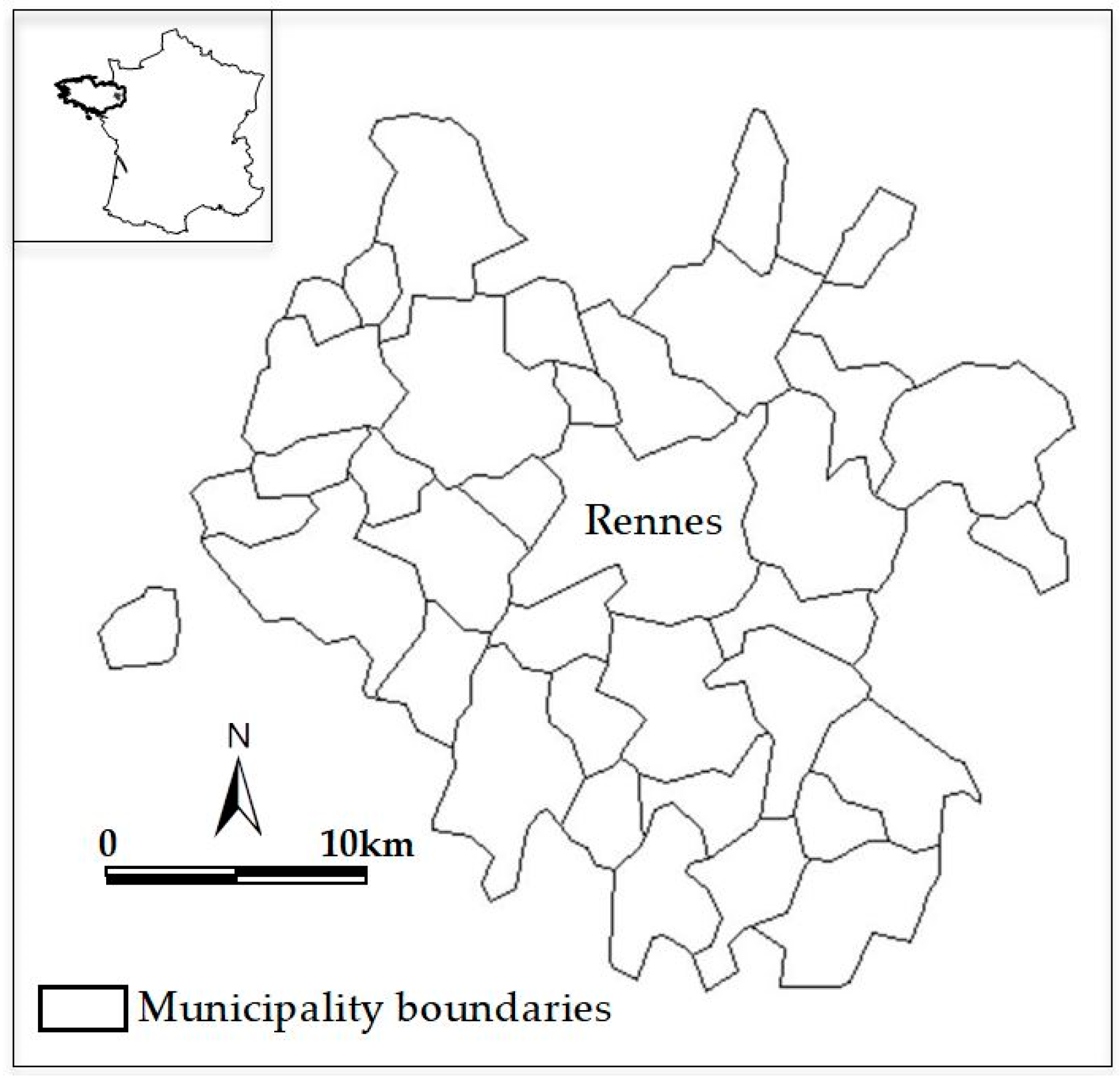
This article uses three terms to describe time: extent, interval, and duration [33]. Temporal extent is the period of time between the first date 2003 and the last date 2018 in a time series data. Interval is a period for which data exist both at an initial date and at a subsequent date. The calibration interval [T0, T1] was used to parameterize the model, whereas the simulation interval [T1, T2] was used to simulate the future urban growth for the desired simulation date T2. Based on LULC maps for 2003, 2006, 2010, 2011, 2012, and 2015, fifteen training intervals within the time extent were implemented to calibrate the model and then to simulate developed areas for 2018: [2003, 2006], [2003, 2010], [2003, 2011], [2003, 2012], [2003, 2015], [2006, 2010], [2006, 2011], [2006, 2012], [2006, 2015], [2010, 2011], [2010, 2012], [2010, 2015], [2011, 2012], [2011, 2015], and [2012, 2015]. Duration is the amount of time of any interval. Furthermore, the temporal stability and the temporal stationarity terms are used interchangeably to describe the degree to which the rate of the actual land change is still consistent over time extent [33,39,40].
For each simulation, only one single interval using only two input LULC maps from two different training dates can be used for calibrating the model, whereas the start of the simulation interval is also the end of the calibration interval. The calibration of CA-Markov is based on one basis LULC image, which is also the calibration endpoint (T1). Duration is the amount of time of any period. Furthermore, the terms temporal stability, temporal homogeneity, and temporal stationarity are used synonymously to establish the validity of model assumptions, and to explore whether the rate of land change trajectories is still consistent over time [33,39,40,41].
Many land cover datasets and remote sensing images such as CORINE Land Cover database and large-scale 30-m land cover maps are delivered with a certain spatial and temporal accuracy that is often unsuitable for the temporal slight change analysis in an urban landscape. Consequently, the observed change can be simply due to misclassification errors especially in small zones undergoing slow rate of change as in the current research study area. Accordingly, for temporal land change analysis requirements and modeling purposes over fifteen years from 2003 to 2018, all the input LULC maps are performed using image interpretation. The manual digitization of urban areas is carried out from the ESRI’s World Imagery basemap in ArcGIS Online. World Imagery provides satellite and aerial imagery with a ground resolution of 1 m or less, for example, the satellite images used for mapping impervious surfaces in 2018 are provided with an accuracy of 8.5 m and a ground resolution that varies between 30 and 50 cm. In addition to that, increased built-up areas between 2003 and 2018 are mapped using visual interpretation of historical Google Earth’s free and public high-resolution images whose resolution varies according to the source of data.

2.2. Study Area

Rennes Metropolitan is located in the northwest of France (Figure 1). In 2012, it summed up to 705 km2 and had a population of 4,120,717 inhabitants that were dispersed between 37 municipalities. Rennes Metropolitan is one of the booming areas in the west of France. Since the late 50s, Rennes Metropolitan has acquired strong experience in land management and urban planning.

2.3. Dataset and Land Change Analysis

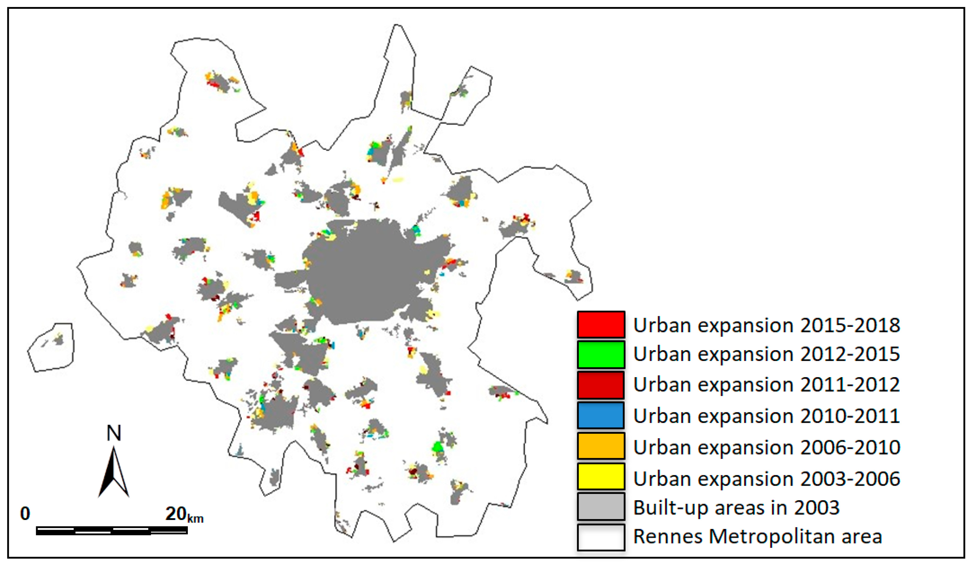
2.3.1. Dependent Variables—Past LUCC

Spatiotemporal urban development dynamic from 2003 to 2018 was analyzed at 15 m resolution using LULC maps for 2003, 2006, 2010, 2011, 2012, 2015, and 2018, which were manually performed using image interpretation technique (Figure 2).
Rennes Metropolitan has known continuous population growth between 2003 and 2018, which led to significant urban expansion and spatial landscape pattern changes (Figure 2). Analysis of historical LUCC between 2003 and 2018 revealed a continuous and significant increase in the developed areas of Rennes Metropolitan with an average annual rate of 115 ha/year (Table 1).
Mainly, urban development has occurred through an edge growth process at the proximity of previously developed areas in order to preserve rural areas and prevent urban sprawl (Figure 2). The analysis of actual spatial growth patterns shows a non-stationary dynamic. In addition to that, the urban development process is not spatially homogeneous and significant differences are observed over time. Moreover, the number of urban patches (NP) has decreased from 240 in 2003 to 218 in 2018, and the Euclidean mean nearest neighbor distance (ENND_MN) has slightly increased from 105 m in 2003 to 137 m in 2018 (Table 1).

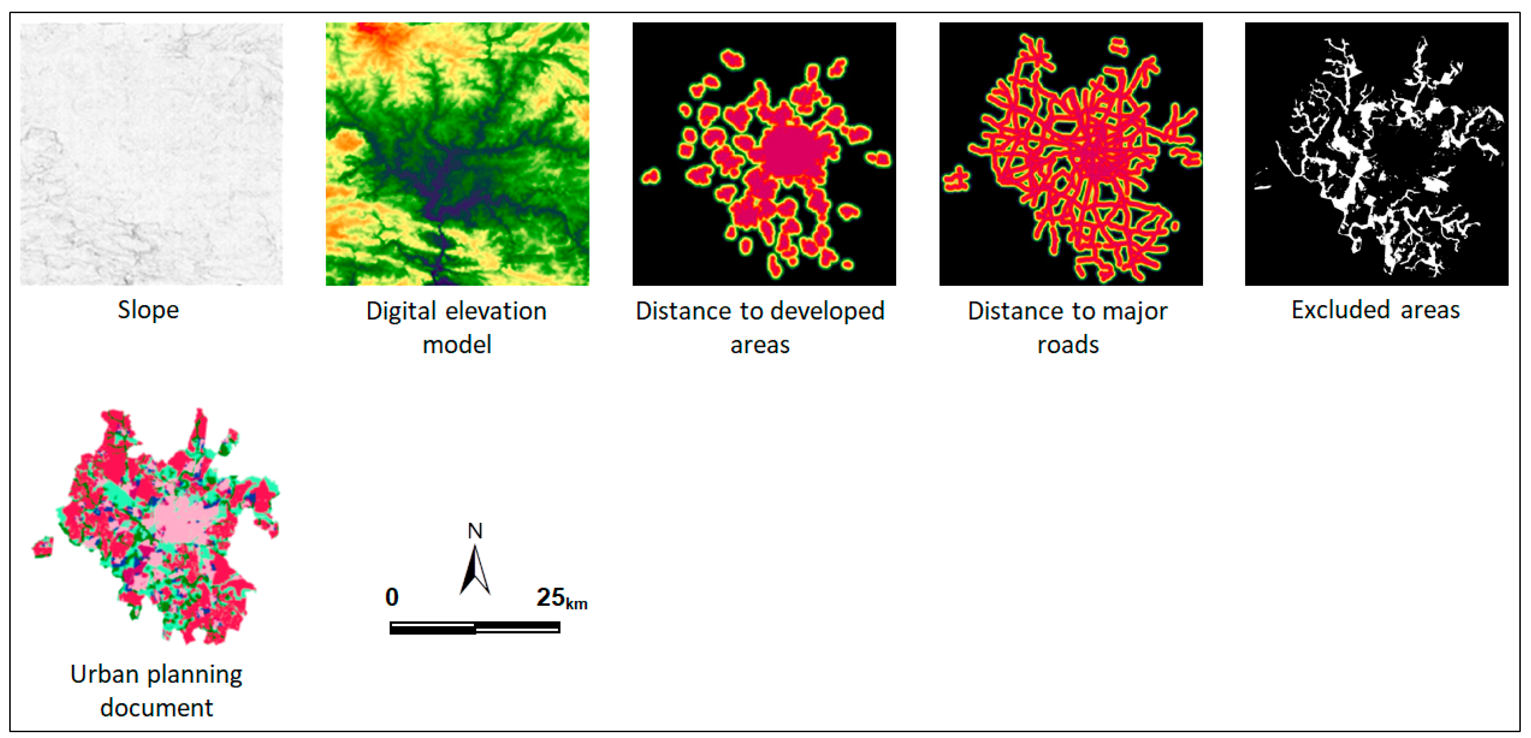
2.3.2. Independent Variables—Constraints and Potential Driving Factors

The input data that are likely to drive the observed urban growth dynamic in Rennes Metropolitan area were prepared to calibrate CA-Markov model and set the simulation rules. These biophysical driving factors covering the same area with the same spatial resolution (15 m) consisted of the existing developed areas, slope, digital elevation model, distance to developed areas, distance to major transportation network, excluded areas from urbanization, and local urban planning document that was designed to establish the general rules concerning land use at the municipality scale (Figure 3). The slope and main road maps are unchanged for all the simulations, regardless of the calibration interval. The distance to developed areas was calculated for the year T1 of every given calibration interval [T0, T1]. The excluded zones included water bodies, wetlands, woodlands, and other protected areas with respect to current land use planning documents and guidelines requirements. The final layer combining all these constraints data was converted into a binary map in order to constraint future development and preserve natural land resources.

2.4. CA-Markov Model

2.4.1. Transition Area Matrix Using a Markovian Process

Land change processes are modeled using stochastic models [41,42]. In fact, Markov processes are stochastic processes in which the state of the system at a given time t+1 is derived from its state at an earlier time t and independent of its history before a spot of time t [39]. Actually, Markov chain is a Markov process which is treated as a series of transitions between certain finite or denumerable possible states of the process. The quantity of land cover change is calculated by means of a transition area matrix using the Markov chain model [33,39,42].
Vt + 1 = Mt × Vt
M   =     1 n P ij     =   [ P 11 P 1 n P ij P n 1 P nn ]
where Vt is the 1-by-n row vector of the input land cover proportion area at an initial time t, Vt+1 is the 1-by-n row vector of the output land cover proportion area at the subsequent time t + 1, M is a n × n transition matrix for an interval t + t + 1, Pij expresses the conditional probability that a pixel of category i at time t transitions to category j by time t + 1, and n is the number of land cover categories.
The conditional probability of transition for a cell transitioning from the category i at time t to the category j at the subsequent time t + 1 is calculated by dividing entry Cij(t) of the raw matrix by the row’s marginal sum. The calibration of the matrix Mt based on a single past time interval using two observed land cover maps allows making projections of future land change.
Pij = Cij j = 1 n Cij
where Cij is the size of area that transitioned from category i at t to category j at time t + 1, j = 1 n Cij is the row’s marginal sum, and n is the number of land cover categories.
The transition probability matrix for the predicted year is firstly calculated based on Equation (4). The original transition probability matrix is obtained based on the two former LULC maps that are used to calibrate the model.
P ( t 2 ) = P ( t 1 ) * P
where P(t2) is the state probability of a point of time, P(t1) is the preliminary state probability, and P is the original transition probability matrix.

2.4.2. CA-Markov Model

Markov model, which is intrinsically aspatial, lacks spatial dependence of geographical cells upon changes in neighboring cells [41]. Therefore, the hybrid CA-Markov model combines the Markov chain that determines the quantity of change and Cellular Automata in order to spatially allocate the estimated change [12,43]. In fact, the Cellular Automata approach adds the spatial contiguity role to the Markov model. The cellular entity changes its state based on both its previous state and adjacent neighbors [43,44]. Therefore, cells that are close to the existing urban areas have a high probability to change [44]. As a matter of fact, the spatial allocation of change using CA-Markov is based on the suitability map. In parallel, other models use the transition potential approach [12,37,38].
Running CA-Markov module in IDRISI program requires inserting the basis land cover image, the Markov transition areas file, transition suitability image collector, and filter type. Criteria that determine the most suitable areas for projected urban development include the excluded protected zones, slope gradient, proximity to roads, and distance to existing developed areas (Figure 2). Proximity to developed areas is calculated for the end point (T1) of the calibration interval [T0, T1]. Additionally, the constraints for urban development are provided in a binary map. Zero is assigned to areas of absolute constraints and 1 corresponds to unconstrained areas which have no impact. The transition potentials are multiplied by the constraints map during the change prediction process. Furthermore, input factors are previously standardized using IDRISI Fuzzy module. The weight assigned to each driver (distance to urban areas in the basis image: 0.772; distance to roads: 0.173; slope: 0.055) are obtained by using the Analytical Hierarchy Process (AHP) method based on a pair-wise comparison matrix [45,46]. The multi-criteria evaluation (MCE) decision support tool is employed to compute transition suitability maps (Figure 4) using standard kernel size of 5 × 5 pixels contiguity filter.

2.5. Accuracy Assessment

The validity of each simulation output is assessed by comparing the predicted to the actual urban areas for 2018. The comparison is carried out based on the quantity, allocation, and spatial patterns disagreements [5,19,20,47,48]. The quantity error is due to the discrepancy between the estimated and real amounts of change. In parallel, the allocation disagreement is due to spatial inconsistency. A three-dimensional table is performed using the reference last calibration date (T1) map which is also the basis land cover image in CA-Markov module, the reference 2018 map, and the predicted 2018 map [49]. The observed change is the union of hits (observed change correctly predicted as change) and misses (observed change but predicted as persistent), whereas the predicted change consists of hits and false alarms (observed persistent but predicted as change) [20,47]. This comparison permits to differentiate between the fits that are due to the presence of persistent cells (null successes) and the agreements that result from the correct predicted change and [7,20,49,50].
The calculation of the error due to quantity (Equation (5)) involves the time duration of the simulation interval (ΔTSimulation = 2018 − T1) in addition to the observed (B) and the predicted (C) annual change rates over the simulation period [T1, 2018].
ErrorQuantity = (B − C) * ΔTSimulation
where ΔTSimulation is the duration of the simulation interval (years), B is the observed annual change rate over the simulation interval (ha/year), and C is the predicted annual change rate over the simulation interval (ha/year).
The majority of the studies dealing with LUCC modeling, especially the accuracy assessment, tighten the analysis of the error disagreement, which may cause some confusions between the real model performance and the temporal non-stationarity of change. As illustrated above (Equation (5)), the error due to quantity involves the actual (B) and the simulated (C) change rate parameters that result from two different and independent processes. In fact, such processes make the analysis of the error due to quantity difficult. Accordingly, the quantity of disagreement can be reformulated for better interpretation and analysis by introducing two additional parameters (Equation (6)). The variable (A–B) is used to compare the actual change between the calibration and the simulation intervals. It allows measuring the temporal non-stationarity assumption of the change rate over the calibration and the simulation intervals. The variable (A–C) allows to evaluate the ability of the Markov process in estimating the appropriate change rate by replicating the calibration past change rate (A) in the simulation period. In fact, the estimated change (C) is determined based on the observed change rate during the calibration interval (A) using the Markov chain model.
ErrorQuantity = [(A − C) − (A − B)] * ΔTSimulation
where ΔTSimulation is the duration of the simulation interval (years), A is the observed annual change rate during the calibration interval (ha/year), B is the observed annual change rate over the simulation interval (ha/year), C is the predicted annual change rate over the simulation interval (ha/year), (A–C) is a measure of the ability of the model to replicate the calibration change rate in the simulation interval, and (A–B) is a measure of the temporal non-stationarity between the calibration and the simulation intervals. (A–B) equals 0 when the two intervals have the same observed change rate.
In parallel to that, a set of seven commonly used spatial metrics is calculated using the FRAGSTATS Spatial Pattern Analysis Program for Categorical Maps [51]. Spatial metrics are implemented to assess the influence of the calibration dataset variability on the spatial configuration accuracy of the model’s projections [52,53]. Selected metrics, which are calculated based on the four cells neighborhood rule, comprise the number of patches (NP), patch density (PD), landscape shape index (LSI), mean patch area (Area-MN), mean Euclidean nearest neighbor distance (ENND-MN), large patch index (LPI), and patch aggregation index (AI).

3. Results

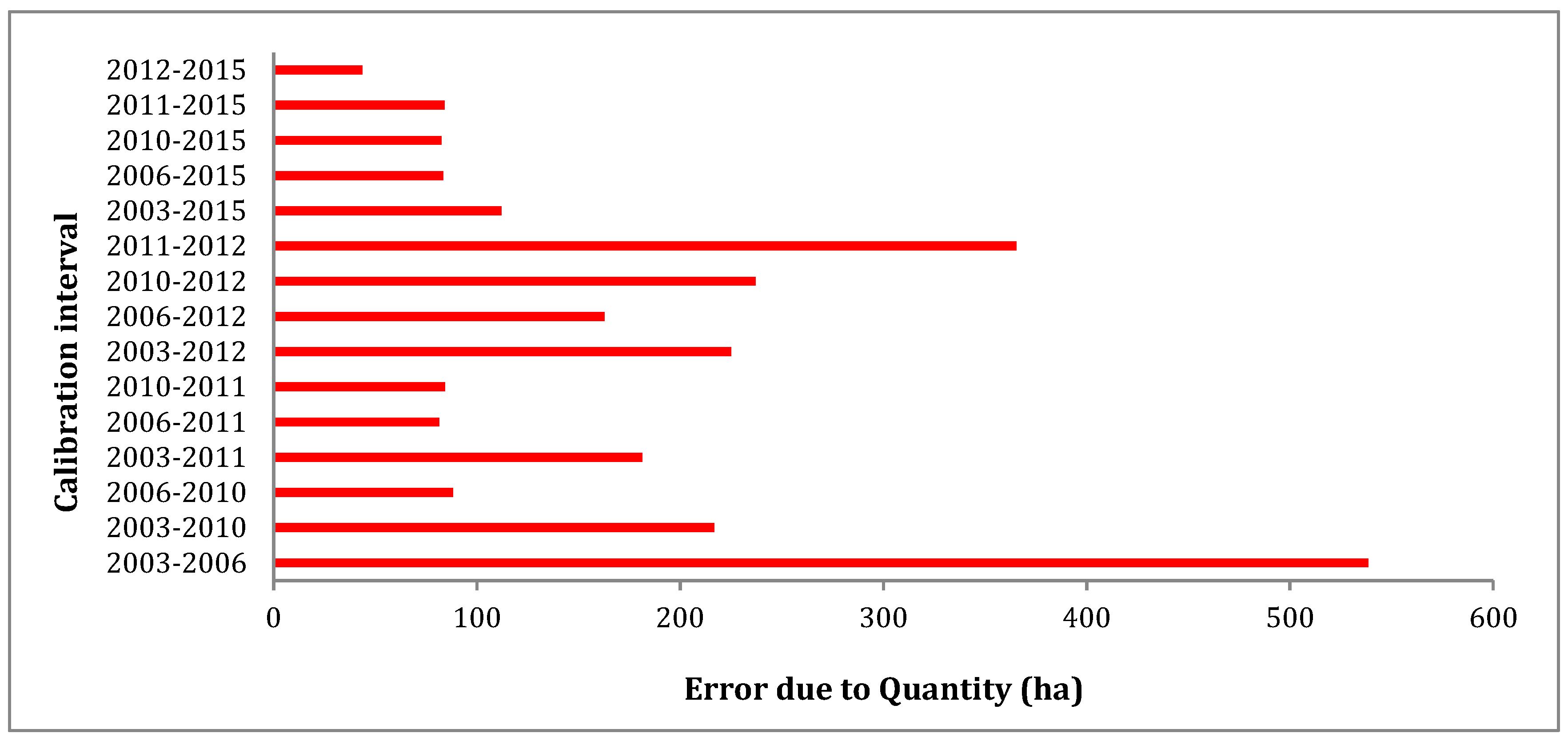
3.1. Quantity of Change Estimate

Table 2 shows the temporal instability of the observed change rate between the calibration (A) and the prediction (B) intervals. The error budget analysis, which was performed at the study area level, revealed a significant variation in the quantity disagreement of the estimated change using the Markov chain model.
The results exhibited an error due to quantity ranging from 45 ha to 540 ha with a standard deviation of 136 ha. The largest error due to quantity (540 ha) was produced by using the calibration interval [2003, 2006] and the simulation interval [2006, 2018] which had the largest time duration (Figure 5). The best score (45 ha) was achieved by using the most recent land cover maps of 2012 and 2015 to calibrate the model.
The results also show the ability of the Markov model in reproducing the observed past change rate in the simulation interval (Table 2). Indeed, the estimated annual growth rate during the simulation interval (C) fit the actual growth rate during the calibration interval (A) for all the simulations. Moreover, the observed annual growth rate during the calibration intervals (A) was higher than the estimated annual growth rate during the prediction interval (C) for all the simulations. The observed difference (A–C) varied from 0 to 2 ha. Therefore, the amount of error due to quantity was primarily determined by the time duration of the simulation interval and the difference of the observed annual change rate between the calibration and the simulation intervals. In addition to that, Figure 6 illustrates a significant variation in the false alarms, misses, and hits. The number of false alarms was slightly greater than the number of misses for all the examined calibration intervals. Accordingly, the Markov model overestimated the amount of predicted developed areas compared to the observed change.
For more details, three categories of calibration intervals could be distinguished based on the distribution of correctness and disagreements. The first group, comprising the calibration interval [2003, 2006], exhibited the maximum number of hits, false alarms, and misses compared to other groups. The second group was composed of five calibration intervals that used 2015 basis land cover image, which was the closest calibration point to the simulation date (2018). This group provided the best fit of 45 ha by producing fewer false alarms and misses. At the same time, it yielded the lowest correctness score. Indeed, the correct predicted cells represented 6% of the total predicted change when using 2015 basis land cover image, whereas it reached 20% when using 2006 basis land cover image. The last category, summing up to nine calibration intervals using land cover basis images of 2010, 2011, and 2012 was characterized by an intermediate score of correctness and errors.

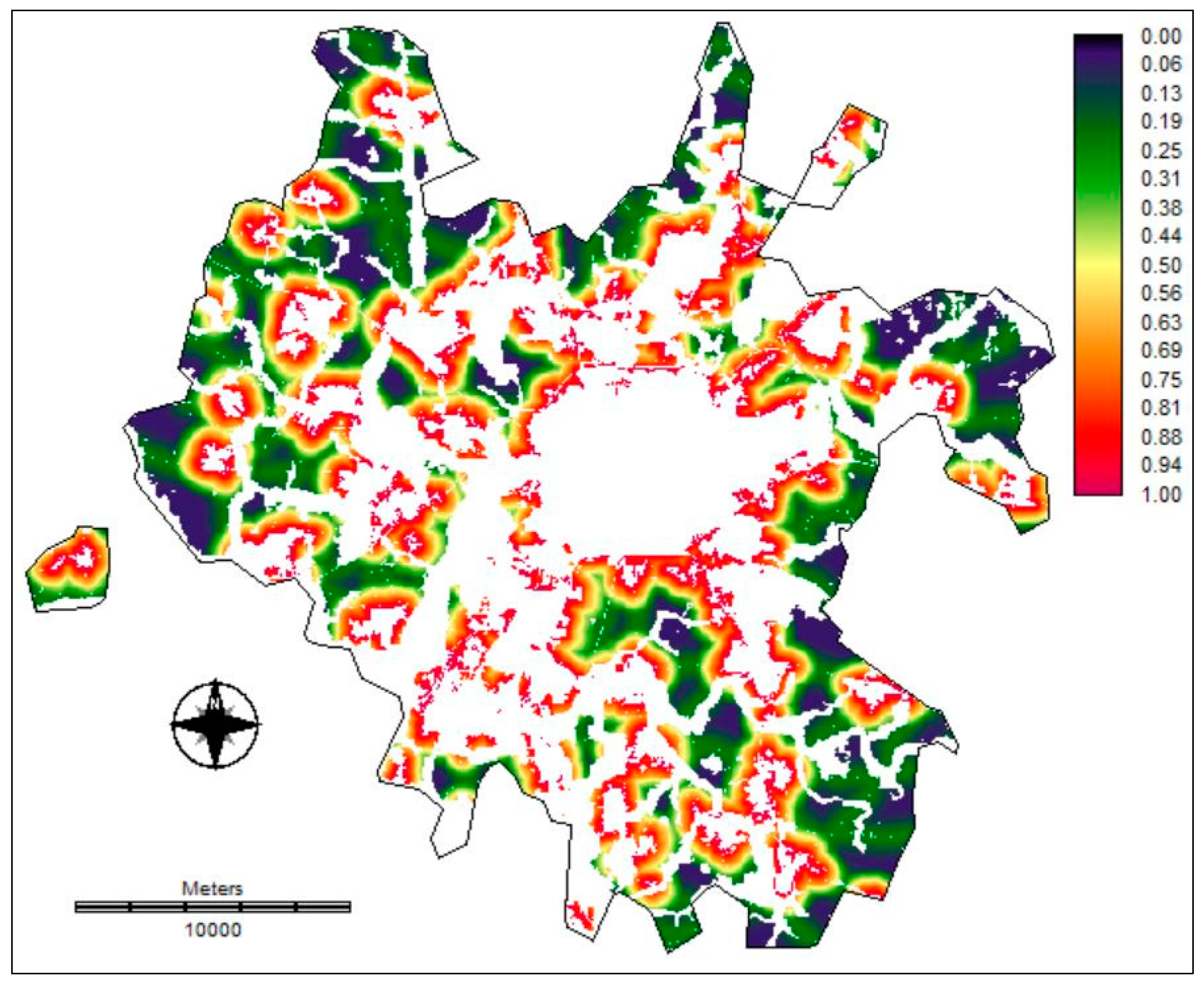
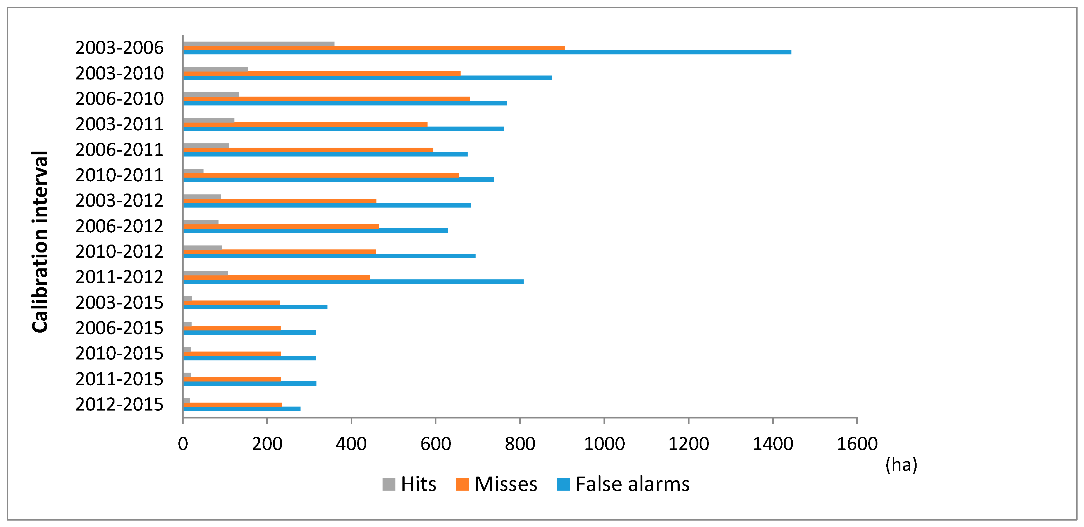
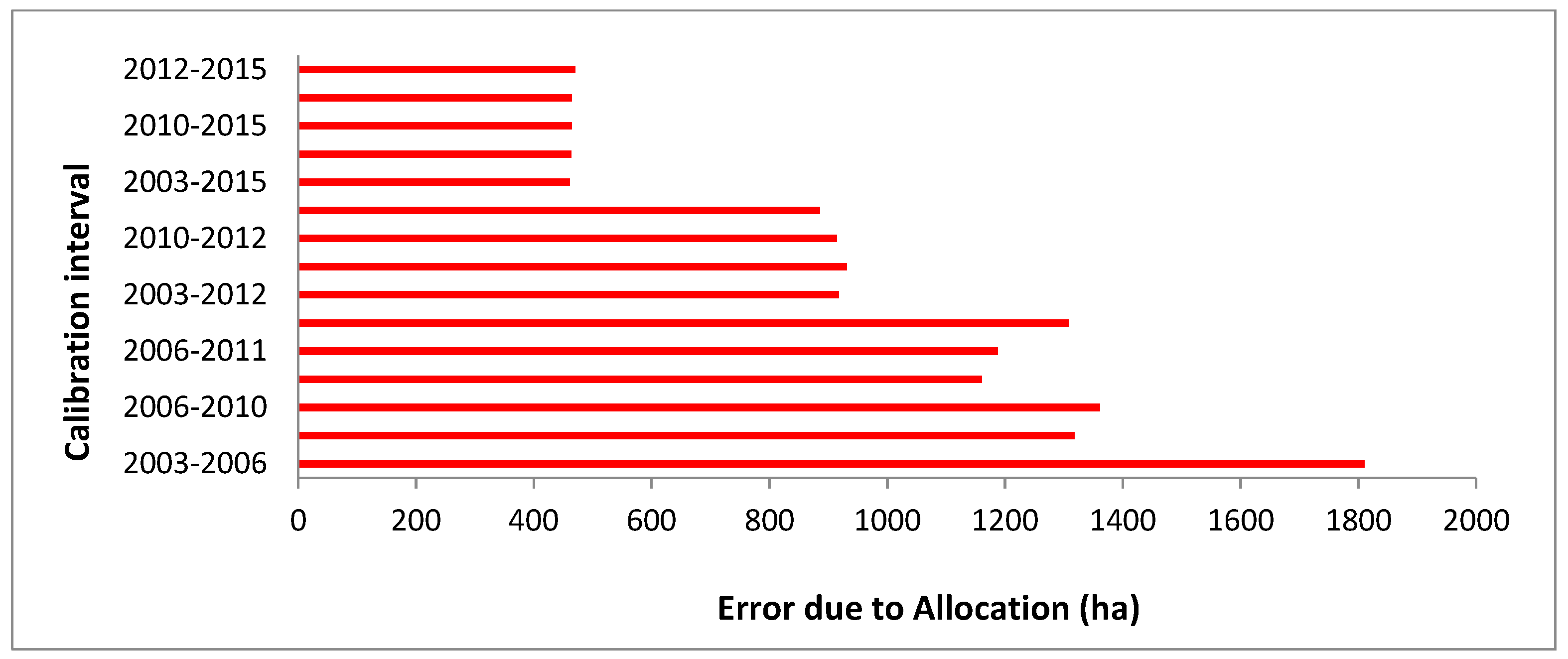
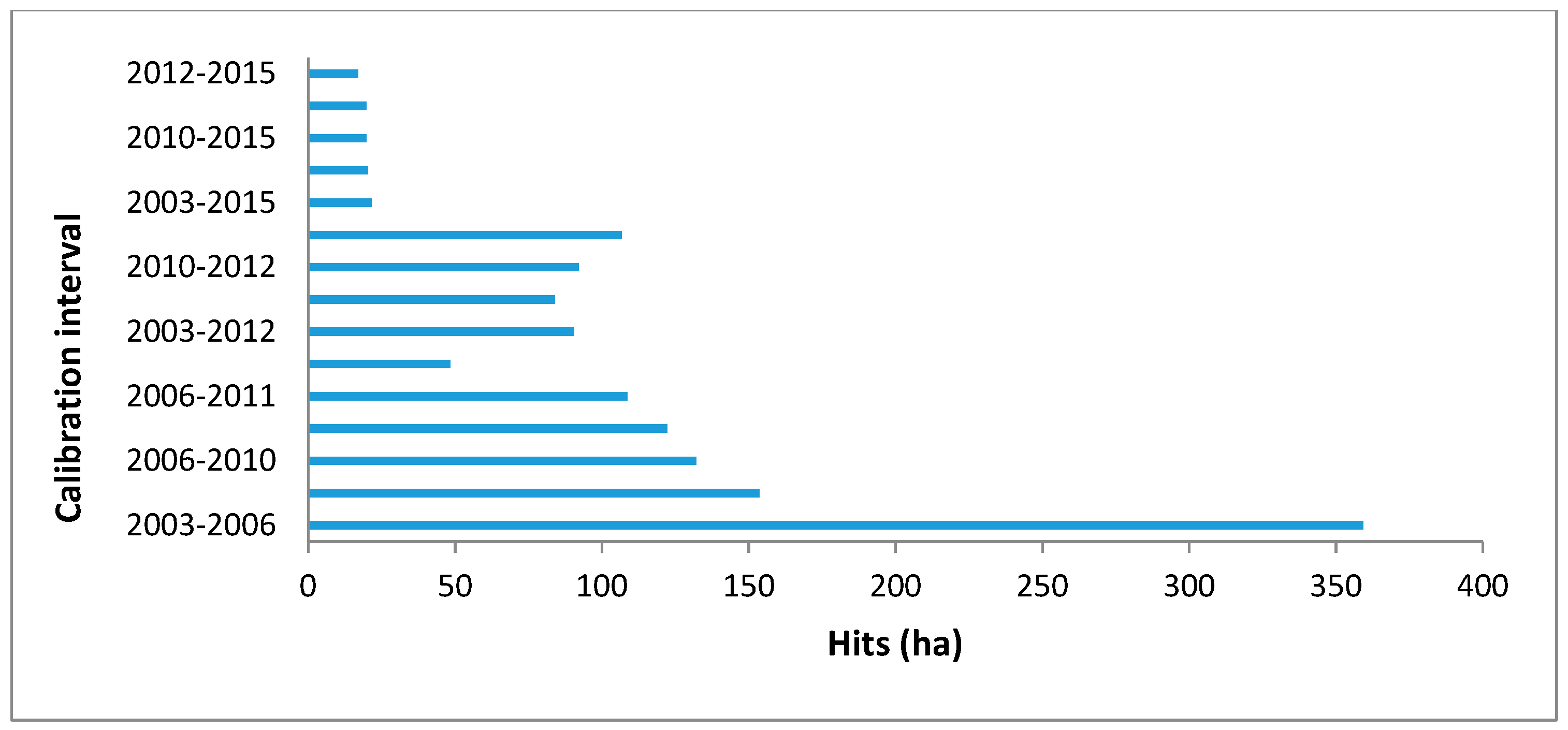
3.2. Spatial Allocation of Change

Simulated developed areas for 2018 using different calibration time intervals [T0, T1] were associated with different amounts of spatial correctness and errors (Table 3). The results point out that both false alarms and misses decreased as the last calibration point (T1) got closer to the target simulation point (T2 = 2018). They also show that the allocation error depended highly on the basis land cover image. For example, the allocation disagreement decreased for 2006, 2010, 2011, 2012, and 2015 basis land cover images. The maximum allocation error, which accounted for 1810 ha, was associated with the calibration interval [2003, 2006].
Table 3 depicts different scores of correctness, errors, and persistent areas depending on calibration intervals. The error due to allocation tended to decrease as the calibration interval involved a more recent date as the endpoint (T1). For example, [2003, 2015], [2006, 2015], [2010, 2015], [2011, 2015], and [2012, 2015] calibration intervals outperformed the remaining intervals that used maps of 2012, 2011, 2010, and 2006 as the basis land cover image.
The calibration interval [2003, 2006] provided the largest allocation error (Figure 7), but also the highest share of hits (Figure 8). The calibration intervals [2003, 2015], [2006, 2015], [2010, 2015], [2011, 2015], and [2012, 2015], which used the most recent basis image (2015), presented the lowest amount of allocation disagreement. At the same time, they yielded the lowest quantity of correctly predicted cells.
Largely, the allocation error still remained the major error component (Figure 9). It varied from 71 to 94% of the total error compared to the quantity disagreement that ranged from 6 to 29%. Moreover, values of the allocation disagreement, which ranged from 461 to 1810 ha, were more dispersed compared to the error due quantity. With a difference of 1349 ha between the minimum and the maximum values, the allocation error presented a standard deviation of 419 ha.
Table 4 shows a comparison between the fifteen simulated urban areas for 2018 using spatial metrics. The results highlight a significant variation, especially in the number of patches (NP), patch density (PD), mean patch area (Area-MN), and mean distance (ENND-MN) between different simulated urban patterns for 2018. Other metrics including landscape shape index (LSI), aggregation (AI), and large patch index (LPI) provided very small variations which should be carefully interpreted by taking into consideration the spatial resolution of the input data.
Figure 10 illustrates that the allocation of the predicted change was characterized by a contiguous spatial pattern, because the actual and the simulated urban development have occurred close to existing developed areas. However, the results indicate that simulated urban areas in 2018 using CA-Markov did not match the spatial configuration of the reference change in terms of the total number of urban patches. Actual urban patches ranged from 240 for 2003 to 218 for both 2005 and 2018, respectively (Table 1). At the same time, Table 4 shows that the number of the simulated urban patches varied from 124 for the calibration interval [2003, 2006] to 173 for the calibration interval [2010, 2011].
The number of the simulated urban patches was smaller than the number of the observed patches compared to the actual situation in 2018 and the basis land cover (T1) image. For example, the simulated patches accounted for 124, while the actual situation in the reference (T2 = 2018) and the basis (T1 = 2006) LULC maps, respectively, accounted for 218 and 228. Actually, the CA-Markov model underestimated the total number of patches by simulating an edge-growth pattern due to the combined effect of the user-defined transition rules and the spatial contiguity filter. CA-Markov has therefore underestimated the number of developed patches by merging closer urban areas regardless of the calibration interval.

4. Discussion

4.1. Quantity of Change Estimate

This current study shows that varying the pair training dates caused significant variations in the estimated amount of the projected developed areas. However, the majority of LUCC modeling approaches, especially those that use Markovian models, assume that the spatiotemporal dynamic of land change still remains homogenous over the calibration and the simulation periods. Such a temporal extrapolation modeling approach may be consistent only when developing the business-as-usual scenario. However, the assumption that future land demand can be solely estimated by extrapolating past tendency could be erroneous in many cases [12]. In fact, estimating the amount of change based on temporal extrapolation modeling process is unable to deal with intermediate changes and temporal discontinuity over time. Actually, demographic, political, socioeconomic, and environmental changes lead to non-stationary urban land demand and spatial patterns over time.
Furthermore, [5] point out that the strict assumption associated with a Markov process can lead to conceptual problems when the calibration and the simulation intervals consist of different time durations. Still, the current study demonstrates that the differences between the calibration and the simulation intervals’ time durations did not matter. For example, the calibration interval [2012, 2015] and the simulation interval [2015, 2018], which had the same short time duration (ΔT = 3), yielded the best quantity agreement (Table 2). However, the quantity disagreement using the calibration interval [2006, 2012] and its corresponding simulation interval [2012, 2018] accounted for 168 ha even if they consisted of the same time duration (ΔT = 6). Actually, the amount of quantity disagreement resulted from the combination of the observed annual change rates during the calibration and the simulation intervals, the simulation time duration, and the predicted annual change rate during the simulation interval (Equation (6)).
The results reveal that a low score of error due to quantity did not automatically mean that the model was efficient enough (Equation (6)). In fact, the error due to quantity provides a useful measure of model performance only if the observed annual change rate remains stationary over the calibration and the validation intervals (A − B = 0). Conversely, the calibration intervals [2006, 2010], [2006, 2012], [2006, 2015], [2010, 2015], [2011, 2012], [2011, 2015] and [2012, 2015] had A = C, which means that the Markov model performed perfectly in estimating the appropriate annual change rate. In addition to that, the predicted change rate fit the actual change rate during the calibration period. In this case, the error disagreement was due to the temporal non-stability (A–B) of the urban growth intensity over time. Moreover, the estimated amount of change during the simulation interval using the Markov technique was lower than the baseline for all the calibration intervals. In fact, the difference (A–C) between the observed annual growth rate during the calibration interval (A) and the predicted annual growth rate during the prediction interval (C) showed that the Markov method tended to underestimate the amount of the predicted developed areas.
Systematically, many studies that deal with LUCC modeling validation techniques under the stationarity assumption [5,47] underestimate the real predictive performance of models in replicating the past amount of change in the future. In fact, they usually attribute the error due to the temporal non-stationarity of land change to the model limitations. Accordingly, the proposed method to analyze the quantity disagreement components will be useful in assessing the real accuracy of models. It permits to distinguish between the capacity of the adopted modeling framework in reproducing past tendency and the non-stationarity of land change over the calibration and simulation time intervals. The modeling framework includes not only the model’s behavior but also the modeler’s methodological choices, particularly in determining the simulation transition rules using a knowledge-driven approach such as in CA-Markov change potential evaluation. In addition to that, assessing LUCC simulation accuracy is a critical task which requires high change detection accuracy. In fact, misregistration of the satellite images and misalignment of different data sources drop the accuracy of the detected change [13,20]. Thus, the current study used manual image interpretation for mapping historical LUCC because mismatched data and classification errors will ultimately lead to inaccurate predictions and bias in the model performance assessment, especially in landscapes experiencing small changes.

4.2. Spatial Allocation of Change

The results point out that using different calibration time intervals [T0, T1] resulted in significant variations in the amount of hits and allocation disagreement. The error due to allocation, which depends on the spatial allocation process that is based on the change potential map, tended to decrease as the calibration interval used a recent endpoint reference map (T1). In fact, false alarms and misses dropped as the last calibration point (T1) got closer to the target simulation point (T2). For example, the shortest (ΔTCalibration = 3) calibration interval [2003, 2006], which was associated with the longest (ΔTSimulation = 12) simulation interval [2006, 2018], provided the maximum allocation error, but also the highest share of the correct allocated urban cells. Conversely, all of the calibration intervals that used the most recent basis image (T1 = 2015 and ΔTSimulation = 3) yielded the lowest amount of the misallocation pixels, but also the lowest quantity of hits. Moreover, the allocation error constituted the major error component. It varied from 71 to 94% of the total error, compared to the quantity disagreement that ranged only from 6 to 29%. In addition to that, the values of the allocation disagreement were more dispersed compared to the error due quantity. Therefore, future improvements should focus more on the spatial allocation of the change process.
The spatial patterns of the simulated urban areas using CA-Markov did not perfectly match the spatial configuration of the reference map. Significant variations were observed in the number of patches (NP), mean patch area (Area-MN), and mean distance (ENND-MN) between the different simulated LULC maps for 2018. For example, the number of the simulated urban patches was smaller than the number of the observed ones in the reference land use map (T2), but also smaller than the basis land cover image (T1) itself. In addition to that, the analysis of the spatial metrics showed that as the basis land cover image (T1) got more closer to the simulation target (T2), the number of patches, patch density, and shape index increased, while mean patch area and mean distance decreased.
Overall, the simulated spatial patterns were relatively realistic even they were slightly more compact compared to the actual situation. In fact, the CA-Markov model tends to generate compact spatial patterns by simulating the new individual urban cells mainly adjacent to the existing urban areas in the basic land cover image. For the fifteen simulations, CA-Markov exhibited limitations in dealing with the spatial allocation of the individual patches. This shortcoming can have a negative effect when reproducing past spreading development trends using a path-dependent approach. This behavior of CA-Markov was probably due to the theoretical approach that was applied on the growth modeling using CA models [52]. Actually, a CA-based approach includes feedback mechanisms due to the proximity effect [12,16]. Accordingly, the urbanization level of the local neighborhood of a grid cell strongly influences the allocation of new developed patches [52]. In CA-Markov, the neighborhood filter leads to a suitability score decrease as the candidate pixels are getting away from the existing built-up areas [12]. Nevertheless, the simulated compact spatial patterns cannot be explained only by the neighborhood filter effect. In fact, the effect of the simulation framework related to selected driving forces and change potential evaluation approach should not be neglected. For instance, the current research used the change potential map which was specifically elaborated using a user knowledge-driven approach in order to reproduce the actual dominant edge growth pattern.
Regarding spatial allocation, the simulated change using the CA-Markov model was more determined by the last calibration date rather than the transition that has occurred during the calibration interval. Hence, non-stationary change processes cannot be captured based on the CA-Markov empirical approach. Actually, one of the main differences between CA-Markov and other LUCC software packages within the Idrisi program is the change potential map that is used in the spatial allocation of change. CA-Markov is based on the suitability map, which does not take into consideration the spatial patterns of past changes during the calibration period [12]. In fact, the suitability map is elaborated based on the relationships between the selected explanatory drivers and only one available land use map. According to [37], the reference map used by CA-Markov for transforming and weighting input variables is the state of LULC at the last calibration date. Conversely, the reference map in Multi-Layer Perceptron (MLP), SimWeight, and Logistic Regression (LR) methods corresponds to the transition probability map, which takes into account spatial patterns of past changes from the first to the last calibration dates.

4.3. Implications on the Model Performance and Outputs

Using appropriate time series input data and calibration intervals is extremely important when the objective is to reproduce past change patterns and validate empirically based LUCC model under the hypothesis of temporal homogeneity. Otherwise, significant errors could be induced, especially when past trend-based models are used in the simulation of path-dependent land use scenarios [33]. In fact, the results revealed how outcomes and accuracy scores of the Markov chain and CA-Markov models vary significantly with respect to selected calibration dates. The magnitude of measured residues is largely due to the non-stationarity of the observed land change over the calibration and the prediction intervals rather than the inadequacy of Markov model. Therefore, the validation interval needs to be consistent with the calibration interval in terms of the amount and spatial patterns of change. This requirement will lead to a better evaluation of the model ability in reproducing past-trend dynamics. [27] propose the estimation of the degree of significance of selected training dates using long time series of LULC maps. Subsequently, several calibration intervals should be included based on the research objective, types of errors to be assessed (quantity, allocation, and spatial patterns), and trade-offs in the model accuracy. The variation in the size and intensity of change across time intervals has to be determined. For instance, the quantitative method developed by [54] can be employed to unify size measurements and stationarity of land changes by time interval. In addition to that, the comparison of Markov matrices associated with different time intervals can be performed using a variety of methods that have been developed to adjust conditional probabilities of transitions (Equation (3)) to represent an equivalent duration [33,39,40,41].
The assessment of spatial allocation requires that the validation interval should match the reference quantity during the calibration interval because of the sensitivity of the pattern metrics to the quantity of each category [11]. According to [55], evaluating spatial allocation accuracy of models is difficult when the quantity error is large. Thus, the ability of models to predict spatial allocation can be better assessed when the quantity of change is correctly estimated [55]. For example, the calibration interval [2012, 2015], which yields the least quantity error, can be used to examine the ability of the model to replicate past spatial patterns in the prediction interval [2015, 2018]. Furthermore, artificially simulated images with specific properties can also be generated in case of lack of actual calibration data that are required to assess the model’s performance in reproducing specific aspects of past changes.
Spatiotemporal non-stationarity of LUCC still remains a complex issue. It involves several parameters including selected calibration time points (long vs. short time duration), input calibration data characteristics (spatial and thematic accuracy), scale of investigation, and underlying processes (global vs. local approach). According to [53], low spatial resolution and thematic accuracy may result in a more generalized structure of the mapped urban land cover objects, thus leading to an overestimation of landscape homogeneity. Conversely, relevant structures may get lost in a highly heterogeneous pattern due to a detailed landscape classification [53].
The number of training dates and the duration of calibration intervals depend on the research objective, observed intensity, and spatial patterns of past change, availability of data, and model inputs requirement. In addition to that, it is a necessity to deal with the risk of extrapolating and generalizing the observed change that has occurred during the calibration interval. According to [13], the temporal extent of the calibration period also affects the simulated LUCC results using models that rely on historical data for their calibration. In fact, a long time calibration interval privileges global trends while tending to average out the extreme tendencies [15]. However, fluctuations due to noise or one-off events are more likely to be captured in a short calibration interval. In addition to that, [12] indicated that the suitability approach is likely to perform better and be more stable as the simulation is carried out over a long period with non-stationary change patterns. According to [10], longtime interval might cause a high number of misses, but also a high share of hits. For example, the shortest time calibration interval [2003, 2006], corresponding to the simulation interval [2006, 2018], which was the longest simulation period (∆T = 12), accounted for the highest quantity and allocation errors, but also the highest number of correct predicted cells. However, the shortest calibration interval [2012, 2015], associated with the shortest simulation interval [2015, 2018], yielded the lowest hits but also the lowest quantity and allocation disagreements.
Furthermore, [7] have already developed an assessment framework that represents the ability of multiple human-environmental models in addressing the tridimensional spatial, temporal, and human-decision making real-world complexity. Models with a high value for temporal complexity may incorporate multiple time steps, long duration, and capacity to handle time lags or feedback responses [7]. For instance, the calibration of the SLEUTH CA-based urban growth model [56] requires four reference dates compared to the majority of existing LUCC models that are limited to two calibration dates only. Other simulation tools like Land Change Modeler [20] are calibrated based on one single past time interval using only two reference land cover maps. As pointed out by [15], the temporal resolution of LUCC models includes the number of available calibration dates and time intervals. In fact, [29] and [24] have found that the number of time-points used in the calibration of a CA-based model significantly influences the calibration result.

5. Conclusions

The influence of the non-stationarity of land change on the calibration and the accuracy assessment of the inductive pattern-based LUCC models is seldom addressed in the literature review. Actually, the stationarity of land change over time is frequently assumed in the majority of LUCC modeling studies. Regarding this, this research aimed at informing users on the influence of the calibration interval on the outputs of LUCC models and their validity estimation. In fact, taking into consideration the non-stationarity of the land change dynamic is a requisite to provide better estimation of the predictive performance of path-dependent LUCC models.
The findings, specifically, demonstrate the influence of varying the calibration time points on the simulation of non-stationary urban growth spatiotemporal dynamic using a CA-Markov model. They exhibited significant variations in the quantity and the spatial allocation agreements with respect to the selected key training dates. For all fifteen examined calibration intervals, the results showed that the Markov model performed better in estimating the annual change rate of the urban growth based on historical data. However, the analysis of the simulated spatial patterns showed that the CA-Markov model tended to foster compact urban form. In addition to that, the spatial pattern accuracy of CA-Markov depended highly on the basis land cover image rather than the observed transition during the calibration period.
At last, the study suggests the use of the appropriate calibration and simulation intervals during which the amount and the spatial patterns of change are stationary. It also recommends the distinction between the non-stationarity of the observed real change and the inability of the adopted modeling framework, which includes both the model behavior and the user’s methodological choices, in reproducing past land changes. For that matter, this paper proposes a useful analysis of errors and correctness variations by examining the error budget using different calibration intervals based on historical LULC data.

Funding

This research received no external funding.

Institutional Review Board Statement

Not applicable.

Informed Consent Statement

Not applicable.

Data Availability Statement

Very high resolution satellite data that support the findings of this study are openly available in Google Earth database or ESRI’s World Imagery basemap.

Acknowledgments

The author would like to thank the anonymous reviewers for their helpful and valuable comments and suggestions.

Conflicts of Interest

The author declares no conflict of interests.

References

  1. Brown, D.G.; Walker, R.; Manson, S.; Seto, K. Modeling Land Use and Land Cover Change. In Land Change Science; Springer: Dordrecht, The Netherlands, 2004; Volume 6, pp. 395–409. [Google Scholar]
  2. Masson, V.; Marchadier, C.; Adolphe, L.; Aguejdad, R.; Avner, P.; Bonhomme, M.; Bretagne, G.; Briottet, X.; Bueno, B.; De Munck, C.; et al. Adapting cities to climate change: A systemic modelling approach. Urban Clim. 2014, 10, 407–429. [Google Scholar] [CrossRef]
  3. Mallampalli, V.R.; Mavrommati, G.; Thompson, J.; Duveneck, M.; Meyer, S.; Ligmann-Zielinska, A.; Druschke, C.G.; Hychka, K.; Kenney, M.A.; Kok, K.; et al. Methods for translating narrative scenarios into quantitative assessments of land use change. Environ. Model. Softw. 2016, 82, 7–20. [Google Scholar] [CrossRef] [Green Version]
  4. Houet, T.; Marchadier, C.; Bretagne, G.; Moine, M.P.; Aguejdad, R.; Viguié, V.; Bonhomme, M.; Lemonsu, A.; Avner, P.; Hidalgo, J.; et al. Combining narratives and modelling approaches to simulate fine scale and long-term urban growth scenarios for climate adaptation. Environ. Model. Softw. 2016, 86, 1–13. [Google Scholar] [CrossRef]
  5. Camacho Olmedo, M.T.; Pontius, R.G., Jr.; Paegelow, M.; Mas, J.F. Comparison of simulation models in terms of quantity and allocation of land change. Environ. Model. Softw. 2016, 69, 214–221. [Google Scholar] [CrossRef] [Green Version]
  6. Noszczyk, T. A review of approaches to land use changes modelling. Hum. Ecol. Risk Assess. Int. J. 2019, 25, 1377–1405. [Google Scholar] [CrossRef]
  7. Agarwal, C.; Green, G.L.; Grove, M.; Evans, T.; Schweik, C. A Review and Assessment of Land-Use Change Models: Dynamics of Space, Time and Human Choice; General Technical Report NE-297; U.S. Department of Agriculture, Forest Service, Northeastern Research Station: Madison, WI, USA, 2000. [Google Scholar]
  8. Haase, D.; Schwarz, N. Simulation Models on Human-Nature Interactions in Urban Landscapes: A Review Including Spatial Economics, System Dynamics, Cellular Automata and Agent-Based Approaches. Living Rev. Landsc. Res. 2009, 3, 1–45. [Google Scholar] [CrossRef]
  9. Triantakonstantis, D.; Mountrakis, G. Urban Growth Prediction: A Review of Computational Models and Human Perceptions. J. Geogr. Inf. Syst. 2012, 4, 555–587. [Google Scholar]
  10. Van Vliet, J.; Bregt, A.K.; Brown, D.G.; van Delden, H.; Heckbert, S.; Verburg, P.H. A review of current calibration and validation practices in land-change modeling. Environ. Model. Softw. 2016, 82, 174–182. [Google Scholar] [CrossRef]
  11. Brown, D.G.; Verburg, P.H.; Pontius, R.G., Jr.; Lange, M.D. Opportunities to improve impact, integration, and evaluation of land change models. Curr. Opin. Environ. Sustain. 2013, 5, 452–457. [Google Scholar] [CrossRef]
  12. Mas, J.F.; Kolb, M.; Paegelow, M.; Camacho Olmedo, M.T.; Houet, T. Inductive pattern-based land use/cover change models: A comparison of four software packages. Environ. Model. Softw. 2014, 51, 94–111. [Google Scholar] [CrossRef] [Green Version]
  13. Burnicki, A.C.; Brown, D.G.; Goovaerts, P. Propagating error in land-cover-change analyses: Impact of temporal dependence under increased thematic complexity. Int. J. Geogr. Inf. Sci. 2010, 24, 1043–1060. [Google Scholar] [CrossRef]
  14. Santé, I.; García, A.M.; Miranda, D.; Crecente, R. Cellular automata models for the simulation of real-world urban processes: A review and analysis. Landsc. Urban Plan. 2010, 96, 108–122. [Google Scholar] [CrossRef]
  15. Mas, J.F.; Paegelow, M.; Camacho Olmedo, M.T. LUCC Modeling Approaches to Calibration. In Geomatic Approaches for Modeling Land Change Scenarios; Camacho Olmedo, M.T., Paegelow, M., Mas, J.F., Eds.; Lecture notes in Geoinformation and Cartography; Springer International Publishing AG.: Cham, Switzerland, 2018; Chapter 2; pp. 11–25. [Google Scholar]
  16. Van Vliet, J.; Naus, N.; van Lammeren, R.J.A.; Bregt, A.K.; Hurkens, J.; van Delden, H. Measuring the neighbourhood effect to calibrate land use models. Comput. Environ. Urban Syst. 2013, 41, 55–64. [Google Scholar] [CrossRef]
  17. Chen, Y.M.; Li, X.; Liu, X.P.; Ai, B. Modeling urban land-use dynamics in a fast developing city using the modified logistic cellular automaton with a patch-based simulation strategy. Int. J. Geogr. Inf. Sci. 2014, 28, 234–255. [Google Scholar] [CrossRef]
  18. Bennett, N.D.; Croke, B.F.W.; Guariso, G.; Guillaume, J.H.; Hamilton, S.H.; Jakeman, A.J.; Marsili-Libelli, S.; Newham, L.T.H.; Norton, J.P.; Perrin, C.; et al. Characterizing performance of environmental models. Environ. Model. Softw. 2013, 40, 1–20. [Google Scholar] [CrossRef]
  19. Pickard, B.; Gray, J.; Meentemeyer, R. Comparing Quantity, Allocation and Configuration Accuracy of Multiple Land Change Models. Land 2017, 6, 52. [Google Scholar] [CrossRef] [Green Version]
  20. Aguejdad, R.; Houet, T.; Hubert-Moy, L. Spatial validation of land-use change models using multiple assessment techniques: A case study of transition potential models. Environ. Model. Assess. 2017, 22, 591–606. [Google Scholar] [CrossRef]
  21. Aguejdad, R.; Doukari, O.; Houet, T.; Avner, P.; Viguié, V. Modélisation prospective de l’étalement urbain: Apports et limites des modèles de spatialisation. Application aux modèles SLEUTH, LCM et NEDUM-2D. Cybergeo Eur. J. Geogr. 2016, 782. [Google Scholar] [CrossRef]
  22. Lambin, E.F.; Geist, H.J.; Lepers, E. Dynamics of land-use and land-cover change in tropical regions. Annu. Rev. Environ. Resour. 2003, 28, 205–241. [Google Scholar] [CrossRef] [Green Version]
  23. Kolb, M.; Mas, J.F.; Galicia, L. Evaluating drivers of land-use change and transition potential models in a complex landscape in Southern Mexico. Int. J. Geogr. Inf. Sci. 2013, 27, 1804–1827. [Google Scholar] [CrossRef]
  24. Verstegen, J.A.; Karssenberg, D.; van der Hilst, F.; Faaij, A.P.C. Detecting systemic change in a land use system by Bayesian data assimilation. Environ. Model. Softw. 2015, 75, 424–438. [Google Scholar] [CrossRef] [Green Version]
  25. Eastman, J.R.; van Fossen, M.E.; Solorzano, L.A. Transition Potential Modeling for Land Cover Change. In GIS, Spatial Analysis and Modeling; Maguire, D., Batty, M., Goodchild, M., Eds.; ESRI Press: Redlands, CA, USA, 2005; pp. 357–386. [Google Scholar]
  26. Pérez-Vega, A.; Mas, J.F.; Ligmann-Zielinska, A. Comparing two approaches to land use/cover change modeling and their implications for the assessment of biodiversity loss in a deciduous tropical forest. Environ. Model. Softw. 2012, 29, 11–23. [Google Scholar] [CrossRef]
  27. Paegelow, M.; Camacho Olmedo, M.T.; Mas, J.F.; Houet, T. Benchmarking of LUCC modelling tools by various validation techniques and error analysis. Cybergeo Eur. J. Geogr. 2014, 701. [Google Scholar] [CrossRef]
  28. Bürgi, M.; Hersperger, A.M.; Scheneeberger, N. Driving forces for landscape change—Current and new directions. Landsc. Ecol. 2004, 19, 857–868. [Google Scholar] [CrossRef]
  29. Blecic, I.; Cecchini, A.; Trunfio, G.A. How much past to see the future: A computational study in calibrating urban cellular automata. Int. J. Geogr. Inf. Sci. 2015, 29, 349–374. [Google Scholar] [CrossRef]
  30. Pontius, R.G., Jr.; Huffaker, D.; Denman, K. Useful techniques of validation for spatially explicit land-change models. Ecol. Model. 2004, 179, 445–461. [Google Scholar] [CrossRef]
  31. Wu, X.; Hu, Y.; He, H.S.; Bu, R.; Xi, F. Performance Evaluation of the SLEUTH Model in the Shenyang Metropolitan Area of Northeastern China. Environ. Model. Assess. 2009, 14, 221–230. [Google Scholar] [CrossRef]
  32. Van Vliet, J.; Bregt, A.K.; Hagen-Zanker, A. Revisiting Kappa to account for change in the accuracy assessment of land-use change models. Ecol. Model. 2011, 222, 1367–1375. [Google Scholar] [CrossRef]
  33. Runfola, D.S.M.; Pontius, R.G., Jr. Measuring the temporal instability of land change using the Flow matrix. Int. J. Geogr. Inf. Sci. 2013, 27, 1696–1716. [Google Scholar] [CrossRef] [PubMed]
  34. Wang, H.; Stephenson, S.R.; Qu, S. Modeling spatially non-stationary land use/cover change in the lower Connecticut River Basin by combining geographically weighted logistic regression and the CA-Markov model. Int. J. Geogr. Inf. Sci. 2019, 33, 1313–1334. [Google Scholar] [CrossRef]
  35. Müller, D.; Sun, Z.; Vongvisouk, T.; Pflugmacher, D.; Xu, J.; Mertz, O. Regime shifts limit the predictability of land-system change. Glob. Environ. Chang. 2014, 28, 75–83. [Google Scholar] [CrossRef]
  36. Eastman, J.R. IDRISI Selva Help System; IDRISI Selva Version: 17; Clark Labs, Clark University: Worcester, MA, USA, 2012. [Google Scholar]
  37. Camacho Olmedo, M.T.; Paegelow, M.; Mas, J.F. Interest in intermediate soft-classified maps in land change model validation: Suitability versus transition potential. Int. J. Geogr. Inf. Sci. 2013, 27, 2343–2361. [Google Scholar] [CrossRef]
  38. Yang, X.; Zheng, X.Q.; Chen, R. A land use change model: Integrating landscape pattern indexes and Markov-CA. Ecol. Model. 2014, 283, 1–7. [Google Scholar] [CrossRef]
  39. Petit, C.; Scudder, T.; Lambin, E. Quantifying processes of land-cover change by remote sensing: Resettlement and rapid land-cover changes in south-eastern Zambia. Int. J. Remote Sens. 2001, 22, 3435–3456. [Google Scholar]
  40. Takada, T.; Miyamoto, A.; Hasegawa, S. Derivation of a yearly transition probability matrix for land-use dynamics and its applications. Landsc. Ecol. 2010, 25, 561–572. [Google Scholar]
  41. Bell, E.; Hinojosa, R. Markov analysis of land use change: Continuous time and stationary processes. Socio. Econ. Plan. Sci. 1977, 11, 13–17. [Google Scholar] [CrossRef]
  42. Lambin, E.F. Modelling Deforestation Processes: A Review; TREES series B: Research Report 1, European Commission, EUR 15744 EN; European Commission: Luxembourg, 1994. [Google Scholar]
  43. Subedi, P.; Subedi, K.; Thapa, B. Application of a Hybrid Cellular Automaton–Markov (CA-Markov) Modeling land use change prediction: A case study of Saddle Creek Drainage Basin, Florida. Appl. Ecol. Environ. Sci. 2013, 1, 126–132. [Google Scholar]
  44. Memarian, H.; Balasundram, S.K.; Talib, J.B.; Sung, C.T.B.; Sood, A.M.; Abbaspour, K. Validation of CA-markov for simulation of land use and cover change in the Langat Basin, Malaysia. J. Geogr. Inf. Syst. 2012, 4, 542–554. [Google Scholar] [CrossRef] [Green Version]
  45. Saaty, T.L. The Analytic Hierarchy Process; McGraw-Hill: New York, NY, USA, 1980. [Google Scholar]
  46. Saaty, T.L.; Vargas, L.G. Models, Methods, Concepts and Applications of the Analytic Hierarchy Process; Kluwer: Dordrecht, The Netherlands, 2001. [Google Scholar]
  47. Chen, H.; Pontius, R.G., Jr. Diagnostic tools to evaluate a spatial land change projection along a gradient of an explanatory variable. Landsc. Ecol. 2010, 25, 1319–1331. [Google Scholar] [CrossRef]
  48. Pontius, R.G., Jr.; Millones, M. Death to Kappa: Birth of quantity disagreement and allocation disagreement for accuracy assessment. Int. J. Remote Sens. 2011, 32, 4407–4429. [Google Scholar] [CrossRef]
  49. Pontius, R.G., Jr.; Peethambaram, S.; Castella, J.C. Comparison of three maps at multiple resolutions: A case study of land change simulation in Cho Don District, Vietnam. Ann. Am. Assoc. Geogr. 2011, 101, 45–62. [Google Scholar] [CrossRef]
  50. Ahmed, B.; Ahmed, R.; Zhu, X. Evaluation of Model Validation Techniques in Land Cover Dynamics. Int. J. Geo. Inf. 2013, 2, 577–597. [Google Scholar] [CrossRef]
  51. McGarigal, K.; Cushman, S.A.; Neel, M.C.; Ene, E. FRAGSTATS: Spatial Pattern Analysis Program for Categorical Maps; Computer Software Program Produced by the Authors at the University of Massachusetts; University of Massachusetts: Amherst, MA, USA, 2002. [Google Scholar]
  52. Herold, M.; Goldstein, N.C.; Clarke, K.C. The spatiotemporal form of urban growth: Measurement, analysis and modeling. Remote Sens. Environ. 2003, 86, 286–302. [Google Scholar]
  53. Herold, M.; Couclelis, H.; Clarke, K.C. The role of spatial metrics in the analysis and modeling of urban land use change. Comput. Environ. Urban Syst. 2005, 29, 369–399. [Google Scholar] [CrossRef]
  54. Aldwaik, S.Z.; Pontius, R.G., Jr. Intensity analysis to unify measurements of size and stationarity of land changes by interval, category, and transition. Landsc. Urban Plan. 2012, 106, 103–114. [Google Scholar] [CrossRef]
  55. Pontius, R.G., Jr.; Castella, J.C.; de Nijs, T.; Duan, Z.; Fotsing, E.; Goldstein, N.; Kok, K.; Koomen, E.; Lippitt, C.D.; McConnell, W.; et al. Lessons and Challenges in Land Change Modeling Derived from Synthesis of Cross-Case Comparisons. In Trends in Spatial Analysis and Modeling; Behnisch, M., Meine, G., Eds.; Geotechnologies and the Environment; Springer International Publishing AG.: Cham, Switzerland, 2018; Volume 19, pp. 143–164. [Google Scholar]
  56. Clarke, K.C.; Hoppen, S.; Gaydos, L. A self-modifying cellular automaton model of historical urbanization in the San Francisco Bay area. Environ. Plan. B Plan. Des. 1997, 24, 247–261. [Google Scholar] [CrossRef] [Green Version]
Figure 1. Rennes Metropolitan area.
Remotesensing 13 00468 g001
Figure 2. Urban development patterns between 2003 and 2018.
Remotesensing 13 00468 g002
Figure 3. Maps of input explanatory variables and constraints.
Remotesensing 13 00468 g003
Figure 4. Suitability map derived from the basis land cover map in 2015 using a multi-criteria evaluation (MCE) tool.
Remotesensing 13 00468 g004
Figure 5. Error due to quantity based on different calibration intervals.
Remotesensing 13 00468 g005
Figure 6. False alarms, misses, and hits using different calibration intervals.
Remotesensing 13 00468 g006
Figure 7. Error due to allocation for 2018 based on different calibration intervals.
Remotesensing 13 00468 g007
Figure 8. Correct predicted change (hits).
Remotesensing 13 00468 g008
Figure 9. Percentage of error due allocation and error due to quantity with respect to total error.
Remotesensing 13 00468 g009
Figure 10. Predicted built-up areas for 2018 using the [2012, 2015] calibration interval.
Remotesensing 13 00468 g010
Table 1. Urban growth in Rennes Metropolitan from 2003 to 2018.
DateArea (ha)Percentage of Landscape (%)NPENND_MNPeriodAnnual Change (ha/Year)Growth Rate (%)
200311,39918.6240105- -
200611,85419.32281132003–20061523.99
201012,30720.12271062006–20101133.82
201112,41720.22211162010–20111100.93
201212,57020.52221152011–20121531.23
201512,86621.02181262012–2015992.36
201813,11821.42181372015–2018841.96
Table 2. Land change rate, time duration, and error due to quantity with respect to different calibration intervals.
Calibration IntervalSimulation IntervalError
PeriodΔT (Year)Observed Rate (A) (ha/Year)PeriodΔT (year)Observed Rate (B) (ha/Year)Predicted Rate (C) (ha/Year)Obs.-Pred. (B–C) (ha/Year)A–B (ha/Year)A–C (ha/Year)EQuantity (ha)
20033152200612105150−45472−540
20062018
2003713020108101129−28291−224
20102018
2003812720117100126−26271−182
20112018
200391302012691129−38391−228
20122018
2003121222015384121−37381−111
20152018
2006411320108101113−12120−96
20102018
2006511320117100112−12131−84
20112018
200661192012691119−28280−168
20122018
200691122015384112−28280−84
20152018
2010111020117100112−1210-2−84
20112018
201021322012691131−40411−240
20122018
201051122015384112−28280−84
20152018
201111532012691153−62620−372
20122018
201141122015384112−28280−84
20152018
2012399201538499−15150−45
20152018
Table 3. Observed vs. predicted changes (ha) based on three-time dimension cross-tabulation.
IntervalsFalse Alarms
2-1-1
Misses
1-2-1
Hits
2-2-1
Persistent
2-2-2
Quantity ErrorTotal ErrorAllocation Error
CalibrationSimulation
2003–20062006–2018144490535911,85453923491810
2003–20102010–201887665915412,30621715351318
2006–201076968113212,3068814501361
2003–20112011–201876258012212,41618113421161
2006–201167659410912,4168112701188
2010–20117396544812,4168413931309
2003–20122012–20186844599112,5692251143918
2006–20126284668412,5691631094931
2010–20126954579212,5692371152915
2011–201280844310712,5693651251886
2003–20152015–20183432312212,866112573461
2006–20153152322012,86684547464
2010–20153152322012,86683547465
2011–20153162322012,86684549465
2012–20152792351712,86644514471
[T0, T1]: calibration interval, [T1, T2]: simulation interval. T2: target simulation date (2018). 2-1-1: persistent no change but predicted as change (false alarms). 1-2-1: observed change but predicted as persistent no change (misses). 2-2-1: observed change correctly predicted as change (hits). 2-2-2: persistent developed areas (null successes).
Table 4. Spatial metrics calculated on the observed and predicted developed areas for 2018 based on different calibration periods.
Calibration IntervalNPPDArea-MNENND-MNLSIAILPI
2003–20061240.11202694.599.73.9
2003–20101460.11032174.999.74.6
2006–20101480.11012175.099.74.6
2003–20111490.11022235.099.74.6
2006–20111460.11012235.199.74.6
2010–20111730.1992155.299.74.6
2003–20121490.11022215.199.74.6
2006–20121460.11012225.299.74.6
2010–20121500.11022215.199.74.6
2011–20121410.11122575.099.74.7
2003–20151580.11002145.499.74.6
2006–20151710.1942005.499.74.6
2010–20151710.1942005.499.74.6
2011–20151710.1942005.499.74.6
2012–20151620.1962065.599.74.6
Publisher’s Note: MDPI stays neutral with regard to jurisdictional claims in published maps and institutional affiliations.

