Article

SMOTE-Based Weighted Deep Rotation Forest for the Imbalanced Hyperspectral Data Classification

1
Department of Remote Sensing Science and Technology, School of Electronic Engineering, Xidian University, Xi’an 710071, China
2
Department of Electronics and Informatics, Vrije Universiteit Brussel, 1050 Brussel, Belgium
3
School of Physical Science and Technology, Northwestern Polytechnical University, Xi’an 710071, China
4
Academy of Advanced Interdisciplinary Research, Xidian University, Xi’an 710071, China
*
Author to whom correspondence should be addressed.
Remote Sens. 2021, 13(3), 464; https://doi.org/10.3390/rs13030464
Submission received: 31 December 2020 / Revised: 22 January 2021 / Accepted: 25 January 2021 / Published: 28 January 2021
(This article belongs to the Special Issue Deep Learning and Feature Mining Using Hyperspectral Imagery)

Abstract

:
Conventional classification algorithms have shown great success in balanced hyperspectral data classification. However, the imbalanced class distribution is a fundamental problem of hyperspectral data, and it is regarded as one of the great challenges in classification tasks. To solve this problem, a non-ANN based deep learning, namely SMOTE-Based Weighted Deep Rotation Forest (SMOTE-WDRoF) is proposed in this paper. First, the neighboring pixels of instances are introduced as the spatial information and balanced datasets are created by using the SMOTE algorithm. Second, these datasets are fed into the WDRoF model that consists of the rotation forest and the multi-level cascaded random forests. Specifically, the rotation forest is used to generate rotation feature vectors, which are input into the subsequent cascade forest. Furthermore, the output probability of each level and the original data are stacked as the dataset of the next level. And the sample weights are automatically adjusted according to the dynamic weight function constructed by the classification results of each level. Compared with the traditional deep learning approaches, the proposed method consumes much less training time. The experimental results on four public hyperspectral data demonstrate that the proposed method can get better performance than support vector machine, random forest, rotation forest, SMOTE combined rotation forest, convolutional neural network, and rotation-based deep forest in multiclass imbalance learning.

1. Introduction

Hyperspectral imagery is simultaneously obtained by remote sensors in dozens or hundreds of narrow and contiguous wavelength bands [1,2,3,4,5]. Compared with traditional panchromatic and multispectral remote sensing images, hyperspectral imagery carry a wealth of spectral information, which enables more accurate discrimination of different objects. Consequently, in recent years, hyperspectral imagery has gained extensive attention for a variety of applications in Earth observations [1,6,7,8,9,10], such as urban mapping, precision agriculture, and environmental monitoring [11,12,13,14,15]. The hyperspectral image classification is a significant research topic and it centers on assigning class labels to pixels. Class distribution, i.e., the proportion of samples belonging to each class, plays an extremely important part in classification research. Some traditional classification methods, such as maximum likelihood classification [16], support vector machine (SVM) [17] and artificial neural network [18], have acquired satisfactory performance on the balanced hyperspectral data.
However, since the hyperspectral image scene usually contains many objects of various sizes and sample labeling is difficult in the real world, the class imbalanced is a fundamental problem in hyperspectral image classification [19]. Generally, the majority classes are defined as the classes with a large number of instances while minority classes are the classes with a small number of samples [9]. Because the cost of misclassifying the minority class is usually much higher than the cost of majority classes [20]. With the skewed class distribution, the classifier is inclined to predict that the input instances belong to the majority class to keep high prediction accuracy [20,21,22,23,24]. Such a strategy is not effective for distinguishing the minority classes, even if they are usually foreground classes of interest. Therefore, one of the biggest challenges that machine learning and remote sensing face is how to classify imbalanced data effectively.
Generally, the aim of imbalance learning is to strive for acquiring a classifier that can provide high classification accuracy for the minority class without heavily compromising the accuracy of the majority classes [25,26,27]. Traditionally, the class-imbalance problem has been dealt with either in the data level [28,29,30] or in the algorithm level [31,32,33,34]. The data level focuses on modifying the sample distribution of classes in training sets to reduce the degree of class imbalance, which makes it fit for the classification prediction of the standard algorithm model. The most common method to deal with the imbalance problem in data level is resampling whose major advantages are that no modification to the classifier is needed and the balanced data can be reused in other applications or classification tasks [35,36]. Resampling can be further divided into two types: undersampling [37] and oversampling [38].
  • Undersampling methods: Undersampling alters the size of training sets by sampling a smaller majority class, which reduces the level of imbalance [37] and is easy to perform and have been shown to be useful in imbalanced problems [39,40,41,42]. The major superiority of undersampling is that all training instances are real [35]. Random undersampling (RUS) is a popular method that is designed to balance class distribution by eliminating the majority class instances randomly. However, the main disadvantage of undersampling is that it may neglect potentially useful information, which could be significant for the induction process.
  • Oversampling methods: Over-sampling algorithms increase the number of samples either by randomly choosing instances from the minority class and appending them to the original dataset or by synthesizing new examples [43], which can reduce the degree of imbalanced distribution. Random oversampling is simply copying the sample of the minority class, which easily leads to overfitting [44] and has little effect on improving the classification accuracy of the minority class. The synthetic minority oversampling technique (SMOTE) is a powerful algorithm that was proposed by Chawla [29] and has shown a great deal of success in various applications [45,46,47]. SMOTE will be described in detail in Section 2.1.
The main idea at the algorithm level is to modify the existing classification algorithm model appropriately in combination with the actual data distribution. The typical methods include active learning [48], cost-sensitive learning [49,50], and Kernel-based learning [51].
  • Active learning methods: Traditional active learning methods are utilized to deal with problems with the unlabeled training dataset. In recent years, various algorithms on active learning from imbalanced data problems have been presented [48,52,53]. Active learning is a kind of learning strategy that selects samples from a random set of training data. It can choose more worthy instances and discard the instances which have less information, so as to enhance the classification performance. The large computation cost for large datasets is the primary disadvantage of these approaches [48].
  • Cost-sensitive learning methods: Cost-sensitive learning solves class imbalance problems by using different cost matrices [50]. Currently, there are three commonly used cost-sensitive strategies. (1) The cost-sensitive sample weighting: converting the cost of misclassification into the sample weights on the original data set. (2) The cost-sensitive function is directly incorporated into the existing classification algorithm, which will ameliorate internal structure of the algorithm. (3) The cost-sensitive ensemble: cost-sensitive factors are integrated into the existing classification methods and combine with ensemble learning. Nevertheless, cost-sensitive learning methods require the knowledge of misclassification costs, which are hard to obtain in the datasets in the real world [54,55].
  • Kernel-based learning methods: Kernel-based learning is focused on the theories of statistical learning and Vapnik-Chervonenkis (VC) dimensions [56]. The support vector machines (SVMs), which is a typical kernel-based learning method, can obtain the relatively robust classification accuracy for imbalanced data sets [51,57]. Many methods that combine sampling and ensemble techniques with SVM have been proposed [58,59] and effectively improve performance in the case of imbalanced class distribution. For instance, a novel ensemble method, called Bagging of Extrapolation Borderline-SMOTE SVM (BEBS) was proposed to incorporate the borderline information [60]. However, as this method is based on SVM, it is difficult to implement in a large dataset.
The classification approaches only using the spectral information cannot capture the crucial spatial variability perceived for data, which usually leads to lower performance, especially for the hyperspectral data [61]. Recently, approaches based on deep learning have been developed for the spectral-spatial hyperspectral datasets classification and exhibited their high effectiveness and performance [61,62]. Deep learning is an emerging method that has achieved excellent performance in hyperspectral image classification with sufficient well-labeled data sets [63,64]. Generally, a deep graph structure includes a cascade of layers which is consists of multiple linear and non-linear transformations. Compared with traditional machine learning approaches, deep learning methods can automatically extract informative features from the original hyperspectral dataset by a sequence of hierarchical layers [63]. In addition, deep learning has stronger robustness and higher accuracy than machine learning methods with shallower structures. However, most deep learning approaches, such as the convolutional neural network (CNN), have no algorithmic strategy for dealing with imbalanced data [63,65,66]. As the data set grows larger, the detrimental impact of class imbalance on deep learning methods augments. As mentioned before, the imbalance problem has been comprehensively researched in classical machine learning approaches, nevertheless, it has acquired less attention in the context of deep learning [66]. Besides, the training process of traditional deep learning methods generally consumes much time. The rotation-based deep forest [67], a novel deep learning method, is proposed for the classification of hyperspectral images and achieves satisfactory results with less training time. Nevertheless, this method does not solve the classification problem when the data distribution is imbalanced.
To improve the classification ability of non-ANN based deep-learning approaches for imbalanced hyperspectral datasets, a novel SMOTE-Based Weighted Deep Rotation Forest(SMOTE-WDRoF) algorithm is proposed in this paper. First, the neighboring pixels of instances are introduced as spatial information and multiple new synthetic balanced datasets are created by using the SMOTE algorithm. And then, these datasets are fed into the WDRoF model that consists of the rotation forest and the multi-level cascaded random forests. Specifically, the rotation forest is utilized to generate rotation feature vectors, which are input into the subsequent cascade forest. Moreover, the output probability of each level and the original data are stacked as the dataset of the next level. And the sample weights are automatically adjusted according to the dynamic weight function constructed by the classification results of each level. In summary, the proposed algorithm integrates the advantages of SMOTE, spatial information, and adaptive sample weights. The main contributions of this paper are as follows:
(1)
The proposed SMOTE-WDRoF based on deep ensemble learning combines deep rotating forest and SMOTE internally. It can obtain higher accuracy and faster training speed for the imbalanced hyperspectral data.
(2)
Besides, the introduction of the adaptive weight function can alleviate the defect of SMOTE, which is that SMOTE would generate additional noise when synthesizing new samples.
The remaining part of this paper is summarized as follows. Section 2 describes the related work. Section 3 presents the detail information about the proposed methodology. Then, Section 4 shows the results and discussion. Finally, the conclusions are given in Section 5.

2. Related Works

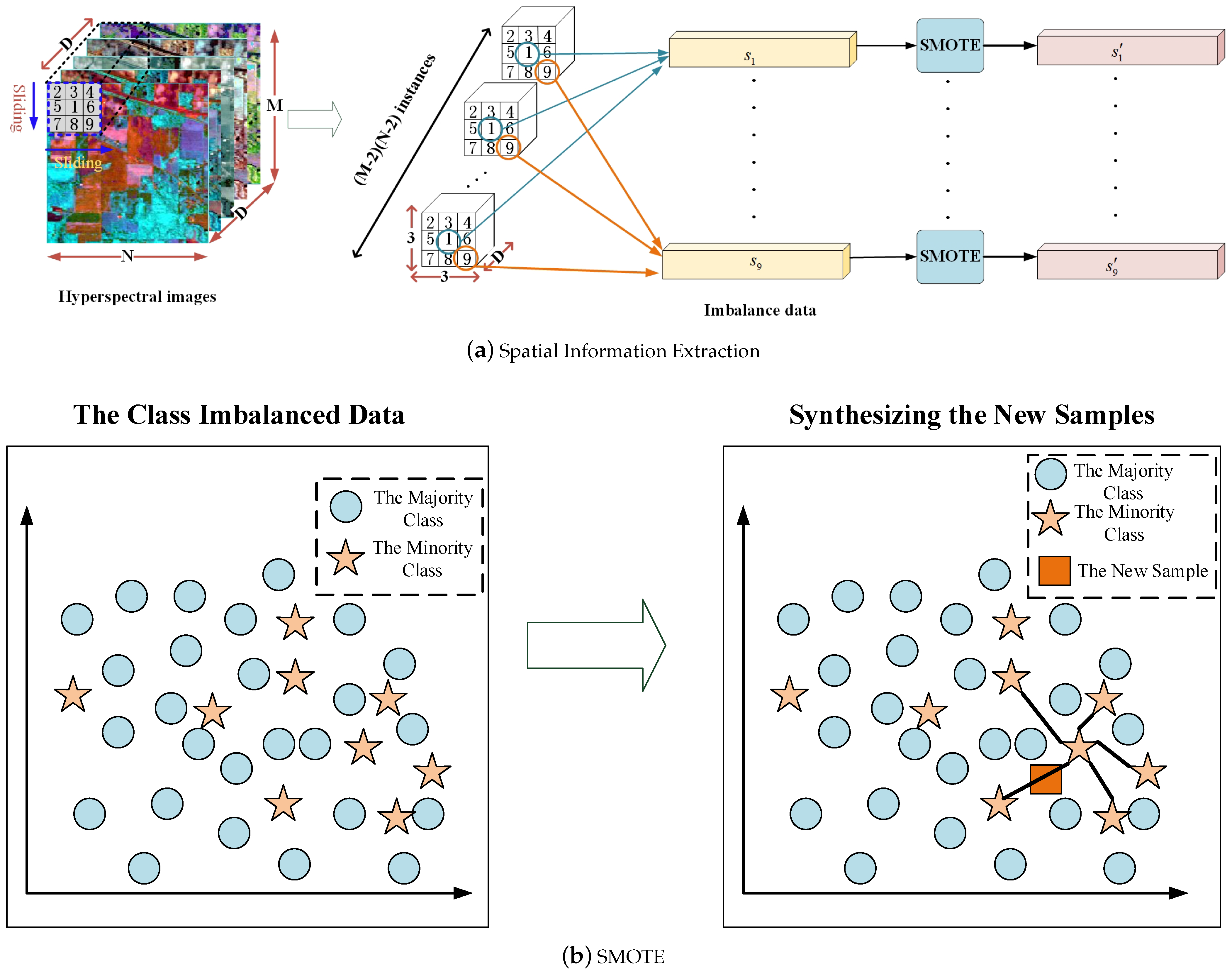
2.1. Synthetic Minority Over-Sampling Technique (SMOTE)

SMOTE, presented by Chawla et al. [29], is the most popular oversampling approach which can solve the overfitting problem. Its main idea is to randomly synthesize new minority samples in the k nearest neighborhood of the selected one through interpolation. It should be noted that the artificial samples are created in the feature space instead of in the data space. The detail process of SMOTE is as follow:
(1)
Calculate k nearest neighbors with minority class samples in accordance with Euclidean distance for each minority instance x i .
(2)
A neighbor x j is randomly chosen from the k nearest neighbors of x i .
(3)
Create a new instances x n e w between x j and x i :
x n e w = x i + δ | x i x j |
where δ is the random number between 0 and 1.

2.2. Random Forest (RF)

Inspired by the bagging algorithm [68], Breiman first proposed random forests [69] in 2001. Its main idea is random sample selection and random feature selection. In RF, all trees are independent of each other, so that the training and testing process are in parallel. Let us suppose a dataset D m with m samples ( X , Y ) , where X R D . First of all, n instances are randomly selected from the original data set D m with replacement. These instances are utilized to build the current decision tree. Second, f features ( f < D ) are first randomly chosen from the original D features. Based on the criterion of Gini impurity or mean squared error (MSE), Classification and Regression Trees (CART) are created. Finally, the classification result is obtained according to the majority voting criterion.

2.3. Rotation Forest (RoF)

Drawing upon the idea of RF, Rodriguez proposed RoF in 2006 [70]. Based on the idea of feature transformation, this algorithm focuses on improving the difference and accuracy of the base classifier. An RoF model of T size is constructed by implementing the following steps.
(1)
Firstly, the feature space F is split into K feature sets which are disjoint and each subset includes N = F / K number of features.
(2)
Secondly, a new training set is obtained by using bootstrap algorithm to randomly selected the 75% of the training data.
(3)
Then, the coefficients a t , g ( g G , t T ) is obtained by employing the principal component analysis (PCA) on each subspace F t , g ( g G , t T ) and the coefficients of all subspaces are organized in a sparse “rotation” matrix R t ( t T ) .
R t = e t , 1 1 e t , 1 N 1 0 0 0 e t , 2 1 e t , 2 N 2 0 0 0 e t , g 1 e t , g N g
(4)
The columns of R t is rearranged by matching the order of original features F to build the rotation matrix R t . Then, construct the new training set S t = [ S t R t , Y t ] , which is used to train an individual classifier.
(5)
Repeat the aforementioned process on all diverse training sets and generate a series of individual classifiers. Finally, the results are obtained by the majority vote rule.

2.4. Rotation-Based Deep Forest (RBDF)

As a simple deep learning model, the rotation-based deep forest (RBDF) includes L level random forests and each level contains w RF models. This approach adopts the output probability of each level as the supplement feature of the next level [67]. The RBDF model contains three steps. First, spatial information is acquired by using a sliding window to extract the neighboring pixels of training samples. Second, the training samples and its neighboring pixels are fed into the RoF model. And each RoF will generate rotation matrices and construct the rotation feature vector. Third, feed the rotation feature vector into an RF model and obtain the classification probability. Then, all the classification probability vectors of level l are averaged to acquire the averaged probability vector which is stacked into the original dataset as the input data of the next level. Finally, the result is generated by finding out the maximum classification probability.

3. Method

In this section, the SMOTE-WDRoF method is proposed to deal with hyperspectral imbalanced data. Firstly, the local spatial structure of instances is introduced and balance datasets are generated by SMOTE, which allows more wealthy information to be obtained from hyperspectral images and alleviates class imbalance in the data level. Then, multiple levels of the forest are utilized to construct the WDRoF model which is the key ingredient of the whole algorithm. More specifically, the rotation forest is utilized to generate rotating feature vectors, which are input into the subsequent cascade forest. Moreover, the output probability of each level and the original data are stacked as the dataset of the next level. And the sample weights are automatically adjusted according to the dynamic weight function constructed by the classification results of each level. The details of the algorithm are as follows.

3.1. Spatial Information Extraction and Balanced Datasets Generation

The object in the image usually contains consistent spatial structure, i.e., neighbor pixels are likely to have the same label. Consequently, spatial-contextual information should be taken into account when classifying. The proposed algorithm combines spatial neighborhood information extraction strategy with SMOTE approach to select informative spatial neighbors and balance the dataset distribution to increase classification accuracy.
First, spatial information is extracted by using a sliding window. Let us assume X R M × N × D is the hyperspectral image, where M , N , D represent the height, width, and the number of spectral bands of the image respectively. The a m , n , d represents the value of the pixel that is located in line m, column n and band d. To obtain the spectral and spatial information of the hyperspectral dataset, the patch is constructed by extracting pixels in a window of size w 1 × w 2 × D and step size 1 with the central pixel. Suppose the spectral vector of a pixel is x R D , the patch A i can be defined as
A i = a ( w 1 b ) ( w 2 b ) a w 1 ( w 2 b ) a ( w 1 + b ) ( w 2 b ) a ( w 1 b ) w 2 a w 1 w 2 a ( w 1 + b ) w 2 a ( w 1 b ) ( w 2 + b ) a w 1 ( w 2 + b ) a ( w 1 + b ) ( w 2 + b )
where w 1 = w 2 = 2 b + 1 , 1 b m i n ( w 1 , w 2 ) / 2 , i ( M w 1 ) ( N w 2 ) . After scanning the whole hyperspectral image, it can be obtained K patches, where K = ( M w 1 ) ( N w 2 ) . Take a 3 × 3 × D sliding window, for example, each sample and its 8 neighboring pixels are extracted, which is shown in Figure 1a. Due to spatial similarity, each instance is generally the same as those of its spatial neighbors and the material fractions are close to each other. Therefore, they have the same label. The hyperspectral imbalance datasets { s 1 , s 2 , , s 9 } denoted as S are formed by extracting the pixels of corresponding positions in all patches and combining the sample labels Y.
Second, according to the proportion of majority class instances to minority class instances, SMOTE oversamples each imbalance data s w ( w 9 ) . As is shown in Figure 1b, the circle and star stand for the majority class samples and minority class instances, respectively. Suppose that the new sample is created from sample x i with T = 5 . SMOTE will randomly choose a sample from the minority class and its nearest five neighbors. Assuming sample x j is selected. The newly synthesized instance highlighted by the square shape is generated between x i and x j by Equation (1). And then the balanced datasets { s 1 , s 2 , , s 9 } denoted S can be obtained.

3.2. Weighted Deep Rotation Forest (WDRoF)

In this part, we propose the WDRoF algorithm, which is shown in detail in Figure 2. This algorithm adopts a multi-level random forest cascade to classify the hyperspectral dataset. Each level of the random forest produces the classification probabilities and misclassification information of the data which are used as guidance information for the next level. More specifically, the classification probabilities form a class vector that is concatenated with original data to constitute input of the next level. And the classification probability of each layer will be applied to all subsequent layers. Furthermore, the misclassification probability is employed to update the sample weight adaptively. When growing a new level, the performance of this level will be evaluated on the test set. If there is no obvious performance gain, the training procedure will finish. Consequently, the number of levels for RF is automatically identified. The implementation steps of WDRoF are as follows.
(1)
The datasets { s 1 , s 2 , , s W } that have been generated by SMOTE are fed into the RoF models where W = w 1 × w 2 . The s w ( w W ) can be written as s w = { X , Y } = { ( x 1 , y 1 ) , ( x 2 , y 2 ) , , ( x K , y K ) } , where K stands for the number of instances. In RoF, we apply PCA for features transformation which is a mathematical transformation method that transforms a set of variables into a set of unrelated ones. Its goal is to obtain the projection matrix Q = [ q 1 , q 2 , , q K ] :
min Q t r ( Q T X X T Q ) s . t . Q T Q = I
First of all, the self-correlation matrix for X is computed:
c o v ( X ) = E [ ( X E [ X ] ) ( X E [ X ] ) T ]
where E [ X ] is the expected number of X and [ · ] T represents transposition. Second, eigen decomposition is applied on c o v ( X ) to calculate its eigenvalues: λ 1 , λ 2 , , λ K and corresponding eigenvectors: α 1 , α 2 , , α K . Finally, the principal component coefficient can be calculated by the following:
E = [ e 1 , e 2 , , e K ] = [ α 1 , α 2 , , α K ] T X
Construct the rotation matrix with Equation (2) and then generate the rotation feature vectors { f 1 , f 2 , , f W } by the RoF.
(2)
The rotation feature vectors { f 1 , f 2 , , f W } are fed into the first level of the random forest and the weight of the sample W e i g h t w , l 1 ( x k ) is set to 1. In level 1, each RF will generate the classification probability and classification error information of each instance for the dataset. All the classification probabilities vector P = { p 1 , p 2 , , p W } of level 1 are averaged to obtain a robust estimation P ¯ :
P ¯ = 1 W w = 1 W p w = 1 W w = 1 W [ 1 N t r e e i = 1 N t r e e I ( h i ( X ) = Y ) ]
where h i represents the ith decision tree output and N t r e e stands for number of decision tree in RF. In addition, according to the classification error, the weights of the sample ( x k , y k ) can be computed
W e i g h t w , l ( x k ) = W e i g h t w , l 1 ( x k ) e x p [ 1 C c = 1 , c y k C ( v w ( x k , c ) ]
where v w ( x k , c ) is the number of votes of any other class with the wth RF model. The weight of a sample will be increased if it is misclassified by the previous level, which makes the sample play a more significant role in the next level and forces the classifier to focus attention on the misclassified samples.
(3)
In the last level, after the average probability vector is calculated, the prediction label is acquired by finding the maximum probability.
y * = a r g m a x w = 1 W I ( v w ( x k ) = c , c 1 , 2 , , C )
The process of the novel SMOTE-WDRoF method is summarized in Algorithm 1.
Algorithm 1: SMOTE-Based Weighted Deep Rotation Forest (SMOTE-WDRoF)
1Input: X R M × N × D : the hyperspectral image; M: the height of the image; N: the width of the image; D: the spectral bands of the image; w 1 × w 2 × D : the size of sliding window; W = w 1 × w 2 ;
2Process:
3form = 1:M do
4for n = 1:N do
5  Obtain K patches { A 1 , , A K } by scanning the image using the sliding
  window with (3)
6end for
7end for
8forw = 1: W do
9 Acquire the imbalanced data s w by extracting the pixels of corresponding
 positions in K patches
10 Input s w into the SMOTE algorithm
11 Construct the balanced data s w
12end for
13Get the balanced datasets { s 1 , , s w , , s W }
Classification:
14forl = 1: L do
15for w = 1: W do
16  Construct the rotation feature vector f w by utilizing RoF algorithm
17  Train the RF model with f w
18  Update each sample weight: W e i g h t w , l ( x k ) W e i g h t w , l 1 ( x k ) with (8)
19  Calculate the the classification probability p w
20end for
21 Obtain the average probability vector P ¯ with (7)
22 Concatenate P ¯ with the input feature vector to constitute input of the next
 level
23end for
24Output: The prediction label y * = a r g m a x w = 1 W I ( v w ( x k ) = c , c 1 , 2 , , C )

4. Experimental Results

4.1. Datasets

Four hyperspectral imagery (http://www.ehu.eus/ccwintco/index.php?title=Hyperspectral_Remote_Sensing_Scenes) with a high imbalance ratio (IR), including Indian Pines AVRIS, Kennedy Space Center (KSC), Salinas and University of Pavia scenes, are adopted to assess the effectiveness of the proposed WDRoF. For the sake of assessing the performance of the classification algorithms objectively, the training data and the test data should be independent. For Indian Pines AVRIS and KSC, 30% of samples of each class are randomly selected to construct the training set, and the remaining 70% of samples from each class constitute the test set. For Salinas and University of Pavia scenes, 5% of samples of each class are chosen to construct the training set, and the remaining samples constituted the test set. Furthermore, if the number of samples in a certain class is less than 100, half of the samples in that class are selected for training and the remaining half for testing. More detailed information related to the number of training and testing instances is listed in Table 1.
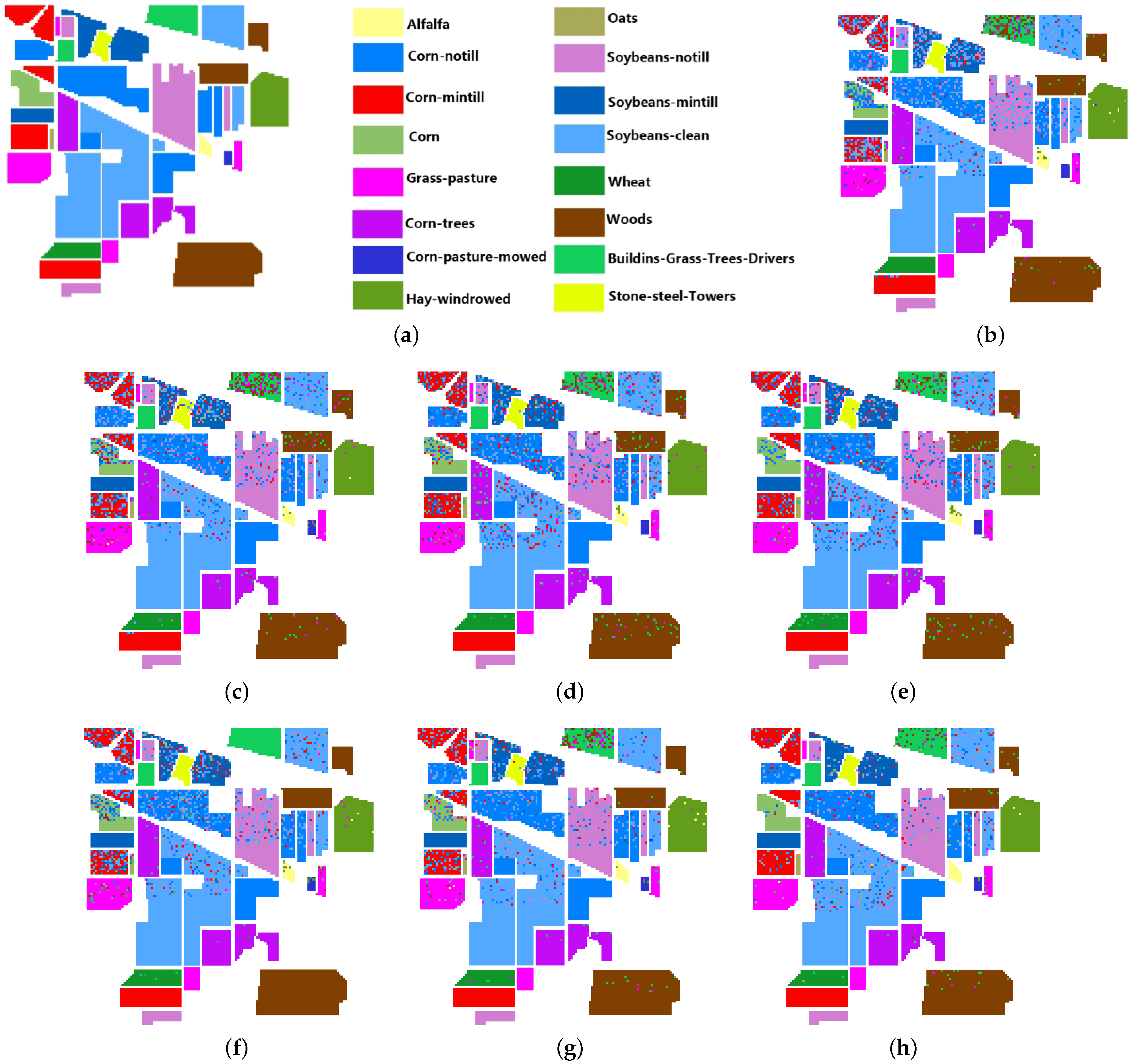
  • Indian Pines AVRIS were obtained employing the National Aeronautics and Space Administration’s Airborne Visible/Infrared Imaging Spectrometer (AVIRIS) sensor and gathered over northwest Indiana’s Indian Pine test site in June 1992. As the high imbalance dataset, Indian Pines AVRIS consists of 145 × 145 pixels and 220 bands covering the range from 0.4 to 2.5 μ m with a spatial resolution of 20 m. There are 16 different land-cover classes and 10,249 samples in the original ground truth. 30% of original reference data are chosen randomly to constitute training dataset and the remaining part constructs test dataset. For Indian Pines AVRIS, if the number of samples is less than 100, such as Oats, half of the samples are randomly chosen to construct training sets. The IR on the training set is 73.6.
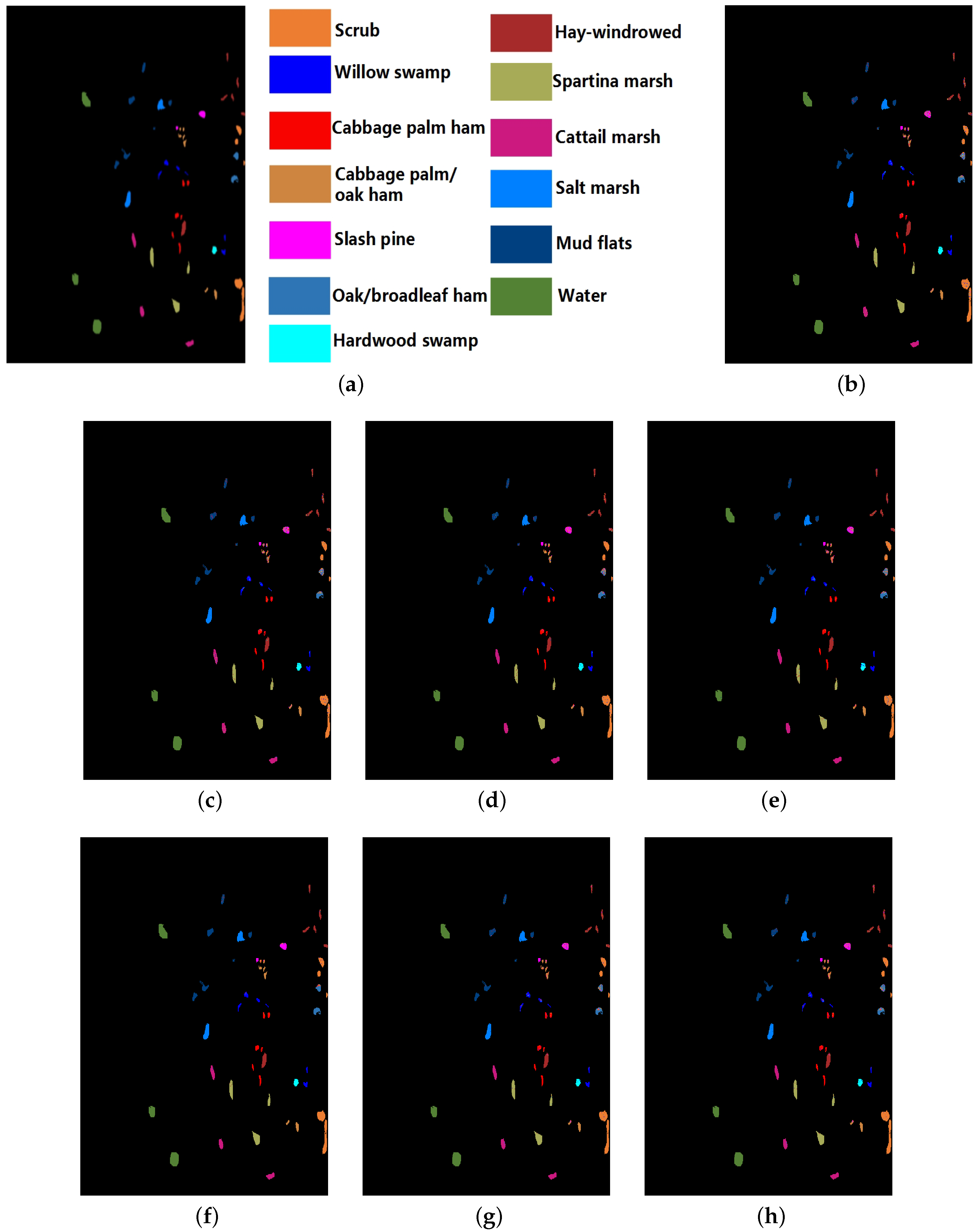
  • KSC was acquired by the Airborne Visible/Infrared Imaging Spectrometer instrument over the Kennedy Space Center (KSC), Florida, on 23 March 1996. The image consists of 512 × 614 pixels with a spatial resolution of 18 m. After removing noisy bands, 176 spectral bands were used for the analysis. Approximately 5208 instances with 13 classes from the ground-truth map. Similar to the setup in the Indian Pines AVRIS image, 30% of pixels per class are randomly selected to constitute the training set, and the others are utilized to construct the test set. The IR on the training set is 8.71.
  • Salinas was gathered by the AVIRIS sensor over Salinas Valley, California with 224 spectral bands. This image consists of 512 × 217 pixels with a spatial resolution of 20 m. The original ground truth also has 16 classes mainly including vegetables, vineyard fields, and bare soils. Training sets are constructed by 8% of its samples chosen randomly from original reference data. The IR on the training set is 12.51.
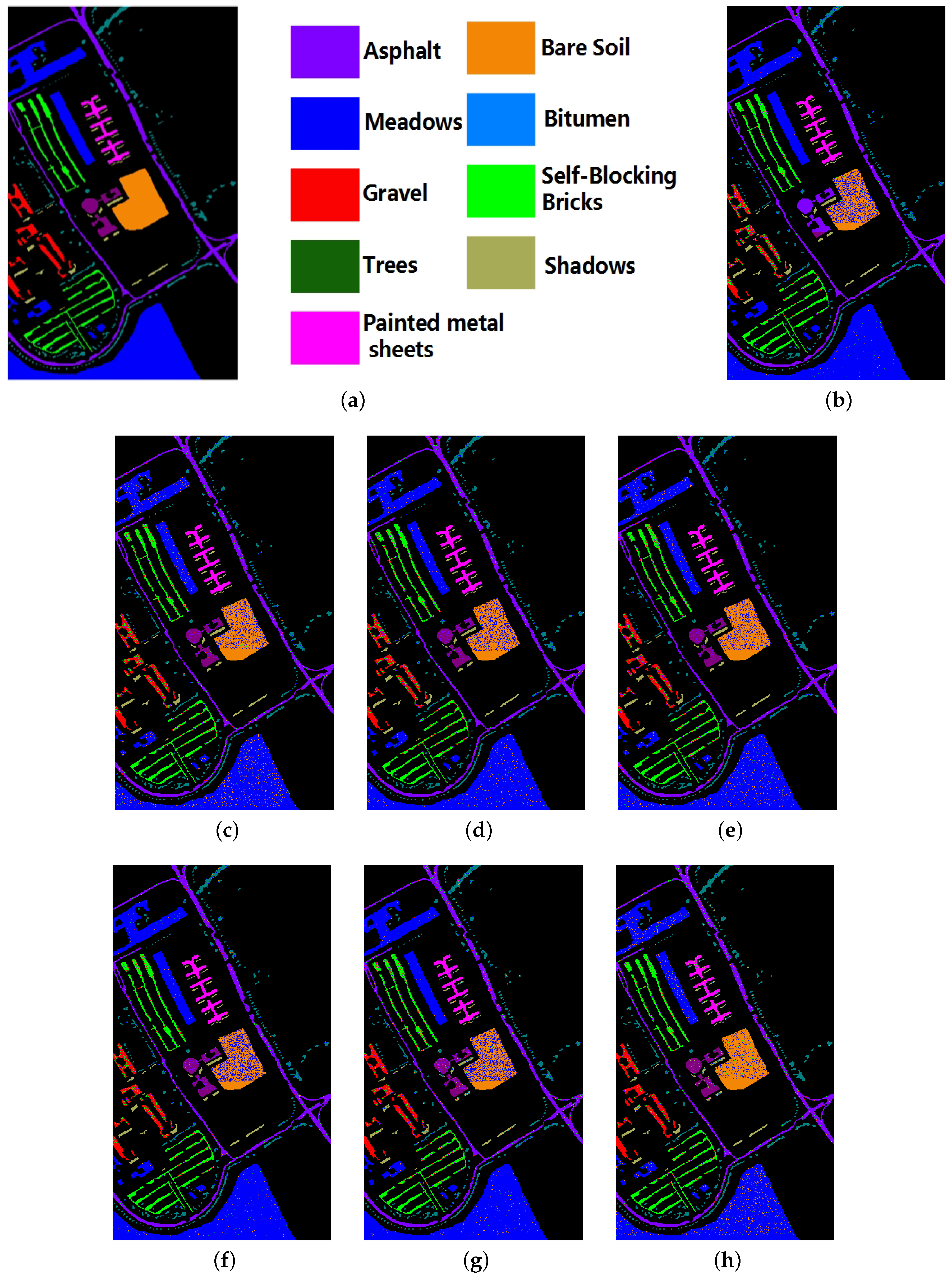
  • University of Pavia scenes covering the city of Pavia, Italy, was gathered by the reflective optics system imaging spectrometer sensor. The data sets consist of 610 × 340 pixels covering the range from 0.43 to 0.86 μ m with a spatial resolution of 1.3 m. There are 16 classes and 42,776 instances in the original ground truth. The training dataset is constituted by 8% of samples that are chosen randomly from original data without replacement. The IR on the training set is 19.83.

4.2. Experiment Settings

In order to demonstrate the advantages of the proposed SMOTE-WDRoF, six popular methods, SVM, RF, RoF, SMOTE combined rotation forest (SMOTE-RoF), Convolutional neural network(CNN) [71], and RBDF is utilized in the comparative analysis. The settings of the six methods are introduced as follows. (1) In the SVM algorithm, the Gaussian function is employed. (2) For RF, the number of trees is twenty. (3) The RoF adopts the PCA transformation and includes 5 trees. The feature dimension of each sample subset is set to 10 and the number of trees. (4) For SMOTE-RoF, the parameter setting is the same as RoF. (5) The settings of CNN are based on reference [71]. (6) For RBDF, there are 20 features in each sample subset of RoF and each RF contains 20 trees. (7) In the proposed SMOTE-WDRoF, each RF also contains 20 trees and 20 features are included in each sample subset for RoF. In addition, for Indian Pines AVRIS and Kennedy Space Center (KSC), the 7 × 7 neighborhood pixels are utilized to classify in RBDF and SMOTE-WDRoF. For Salinas and University of Pavia scenes, these two algorithms use 5 × 5 neighborhood pixels for classification. All the programs are implemented using Python language. The results are generated on a PC equipped with an Intel(R) Core(TM) i5-10200H CPU with 2.4 GHz.

4.3. Assessment Metric

Because the Overall Accuracy (OA) can reflect the overall classification performance of the classifier, it is often adopted to evaluate traditional machine learning classification algorithms. However, when there is a serious imbalance between the data classes, the classification model may be strongly biased towards the majority classes, which results in poor recognition of the minority classes. Therefore, OA is not the most appropriate index to evaluate the model since it might result in inaccurate conclusions [72]. Consequently, this paper adopts five main metrics as performance measures, including the precision, average accuracy, Recall, F-measure, and Kappa.
  • Precision: Precision is employed to measure the classification accuracy of each class in the imbalanced data. The p r e c i s i o n i measures the prediction rate when testing only samples of class i
    p r e c i s i o n i = m i i i = 1 C m j i
    where m i i and m j i stand for the true prediction of the ith class and the false prediction of the ith class into ith class, respectively.
  • Average Accuracy (AA): As a performance metric, AA provides the same weight to each of the classes in the data, independently of the number of instances it has. It can be defined as
    AA = i = 1 C p r e c i s i o n i C
  • Recall: True Positive Rate is defined as recall denoting the percentage of instances that are correctly classified. Recall is particularly suitable for evaluating classification algorithms that deal with multiple classes of imbalanced data [73]. It can be computed as the following equation:
    Recall = 1 C i = 1 C m i i i = 1 C m i j
    where m i j stand for the false prediction of the ith class into jth class.
  • F-measure: F-measure, an evaluation index obtained by integrating precision and Recall, has been widely used in the imbalance data classification [55,74,75]. In the process of classification, precision is expected to be as high as possible, and it is also expected to Recall as large as possible. In fact, however, the two metrics are negatively correlated in some cases. The introduction of F-measure synthesizes the two, and the higher F-measure is, the better the performance of the classifier is. F-measure can be calculated as the following equation:
    F - measure = 2 C i = 1 C R e c a l l i i = 1 C p r e c i s i o n i i = 1 C R e c a l l i + i = 1 C p r e c i s i o n i
    where R e c a l l i can be calculated by n i i i = 1 C n i j .
  • Kappa: The metric that assesses the consistency of the predicted results is Kappa, which checks if the consistency is caused by chance. And the higher Kappa is, the better the performance of the classifier is Kappa can be defined as
    Kappa = O A i = 1 C p i p ^ i 1 i = 1 C p i p ^ i
    where p i and p ^ i stand for the actual sample size of class i and the predicted sample size of class i, respectively.

4.4. Performance Comparative Analysis

In the experiments, the results acquired according to precision, AA, Recall, F-measure, and Kappa are exhibited in Table 2, Table 3, Table 4 and Table 5 for SVM, RF, RoF, SMOTE-RoF, CNN, RBDF and the proposed SMOTE-WDRoF on the four imbalanced hyperspectral datasets. The best results in each hyperspectral dataset are highlighted in bold.

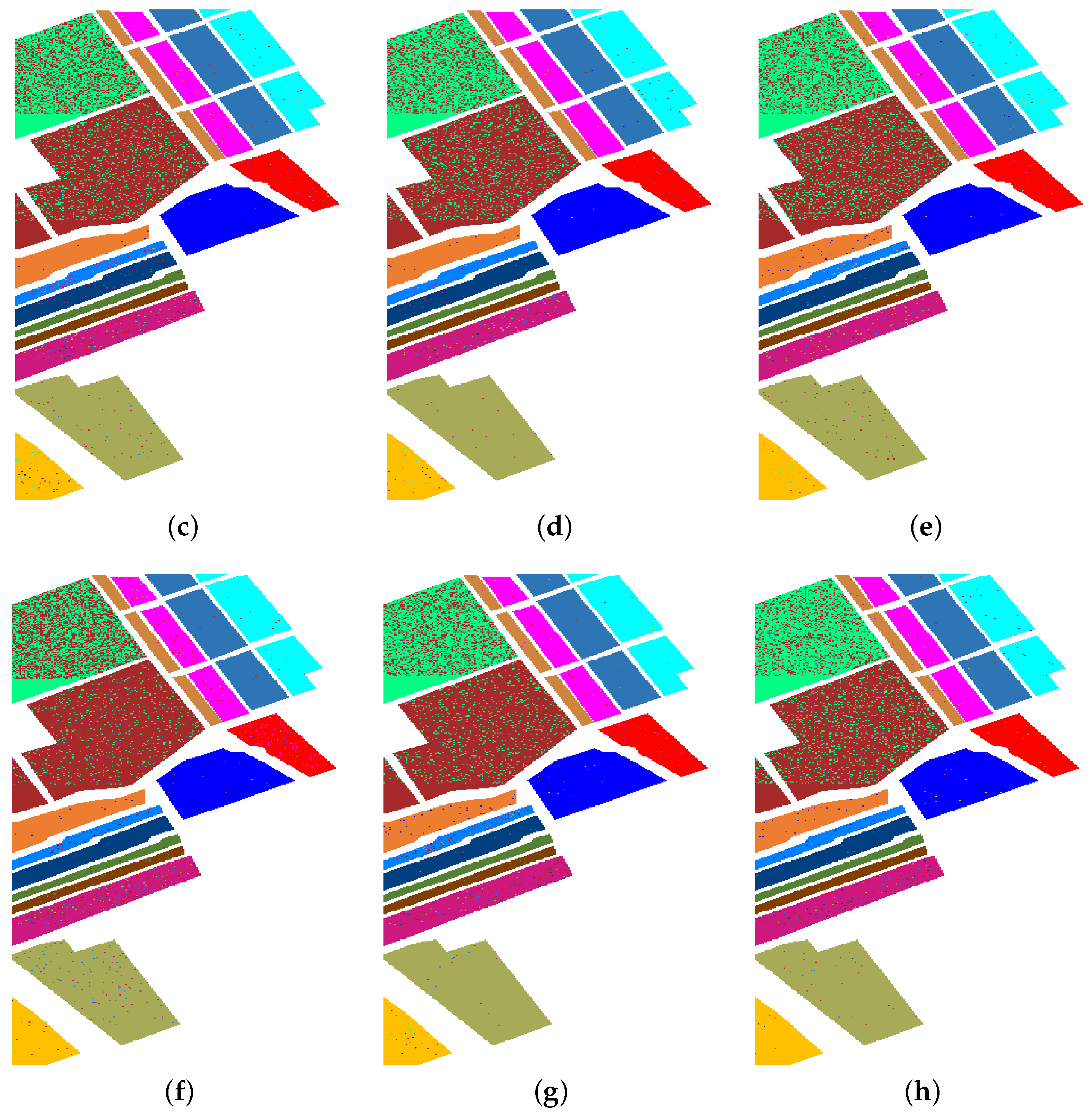
4.4.1. Experimental Results on Indian Pines AVRIS

The results of seven algorithms for Indian Pines AVRIS are listed in Table 2. The first 16 rows are the results of precision, AA, Recall, F-measure, and Kappa coefficients are shown in the last four rows. Among the seven methods, SMOTE-WDRoF achieves the best classification performance in most cases. Because it not only introduces spatial neighborhood pixels and synthesizes samples to increase the sample size and balance the dataset but also adjusts the sample weights adaptively. The proposed method obtains AA of 91.55%, Recall of 91.67%, F-measure of 91.51%, and Kappa of 88.64%, which are the best classification results among the seven methods. Compared with other methods, SMOTE-WDRoF enhances at least 2.61% in AA, 1.90% in Recall, 3.30% in F-measure, and 2.29% in Kappa. Moreover, the SMOTE-WDRoF algorithm obtains 10 of the highest class accuracies among 16 classes in all. Besides, for the class with the least number of training samples, namely Class 9, the accuracy of the proposed algorithm achieves 96.39%, which is at least 14.50% higher than other methods and 53.30% higher at most. The proposed algorithm is superior to other methods in both precisions of the minority classes and overall performance. Figure 3 shows the classification maps obtained by different classification methods for Indian Pines AVRIS. It shows that the proposed SMOTE-WDRoF acquires the best performance on Indian Pines AVRIS dataset.

4.4.2. Experimental Results on KSC

For KSC dataset, the statistical classification results are summarized in Table 3, and the classification results of different methods are shown in Figure 4. As can be observed in Table 3, SMOTE-WDRoF is superior to the other six comparison methods by generating balanced data sets and multi-level forests feature learning. For KSC data containing 13 classes, SMOTE-WDRoF obtained the highest classification accuracy of 10 classes, including multiple minority classes, such as Class 2, Class 4, and Class 7. Furthermore, among all the methods, SMOTE-WDRoF acquires the best statistical results in terms of the AA, Recall, F-measure, and Kappa, and the accuracy of the four metrics is improved by at least 3.63%, 5.20%, 4.54%, and 3.36% respectively. Although RF and RoF algorithms achieve 100.00% accuracy for Class 16, they are far less effective than SMOTE-WDRoF in terms of other performance, especially for the minority classes. In addition, although algorithm SMOTE-RoF has balanced the dataset by synthesizing new samples, its classification performance is worse than SMOTE-WDRoF. In addition, worth noting that SVM algorithm is the worst performer as it pays no attention to the recognition of the minority classes, and its classification accuracy for Class 7 is 0. Therefore, it is demonstrated that the proposed SMOTE-WDRoF has the best classification performance when processing the KSC dataset.

4.4.3. Experimental Results on Salinas

The classification results of seven different methods on the Salinas dataset are shown in Table 4. SMOTE-WDRoF is superior to the other six comparison methods and acquires AA of 95.92%, Recall of 96.05%, F-measure of 95.73%, and Kappa of 91.01%. In addition, SMOTE-WDRoF obtained the highest accuracy for half of the classes on Salinas dataset. For the two classes with the least number of training samples, namely Class 13 and Class 14, the precision of SMOTE-WDRoF reaches 97.92% and 98.81% respectively, which proves its ability to handle the minority classes better than the other comparison methods. Although SMOTE-RF has the highest accuracy in the two classes, the other classes performance of it is not superior. The corresponding classification maps on the data set are illustrated in Figure 5. The experimental results on this dataset testify that the SMOTE-WDRoF shows better classification performance than traditional methods when dealing with class imbalanced data.

4.4.4. Experimental Results on University of Pavia scenes

The results for the proposed SMOTE-WDRoF and six comparison methods on the University of Pavia ROSIS are exhibited in Table 5. Compared with the other methods, SMOTE-WDRoF improves the classification performance by creating new samples to construct the balanced dataset and automatically updating the sample weights based on the classification error information. The proposed SMOTE-WDRoF surpasses RBDF by 2.59%, 2.21%, and 2.32% in terms of Recall, F-measure, and Kappa. Although the AA of the RDBF algorithm is slightly higher than SMOTE-WDRoF, its F-measure that is the synthesis of recall and AA, is significantly lower than SMOTE-WDRoF. While dealing with the minority classes, such as Class 5 and Class 7, the SMOTE-WDRoF performs better than CNN, RDBF, and the other four traditional methods. For visual comparisons, Figure 6 shows the categorization maps of the classification results for all these methods. From Figure 6, we can observe that the proposed method exhibits the best result with least noise. It is obvious that SMOTE-WDRoF obtains the best effect on the University of Pavia ROSIS dataset.

4.4.5. Training Time of Different Deep Learning Methods

The training times of CNN and SMOTE-WDRoF are shown in Table 6. For the CNN, the model needs to continuously adjust the parameters through backpropagation to achieve good performance. Consequently, a large number of parameters need to be calculated in the time-consuming training process. Different from traditional deep learning methods which require backpropagation, the SMOTE-WDRoF needs much less training time. For Indian Pines AVRIS, the training time of CNN is 30,830 s, while the training time of the proposed algorithm is only 3942 s. For KSC, the training time of the proposed algorithm is only one-fourth of that of CNN. For Salinas and University of Pavia ROSIS, SMOTE-WDRoF spends one-sixth and one-twelfth as much time training as CNN, respectively.

4.5. Influence of Model Parameters on Classification Performance

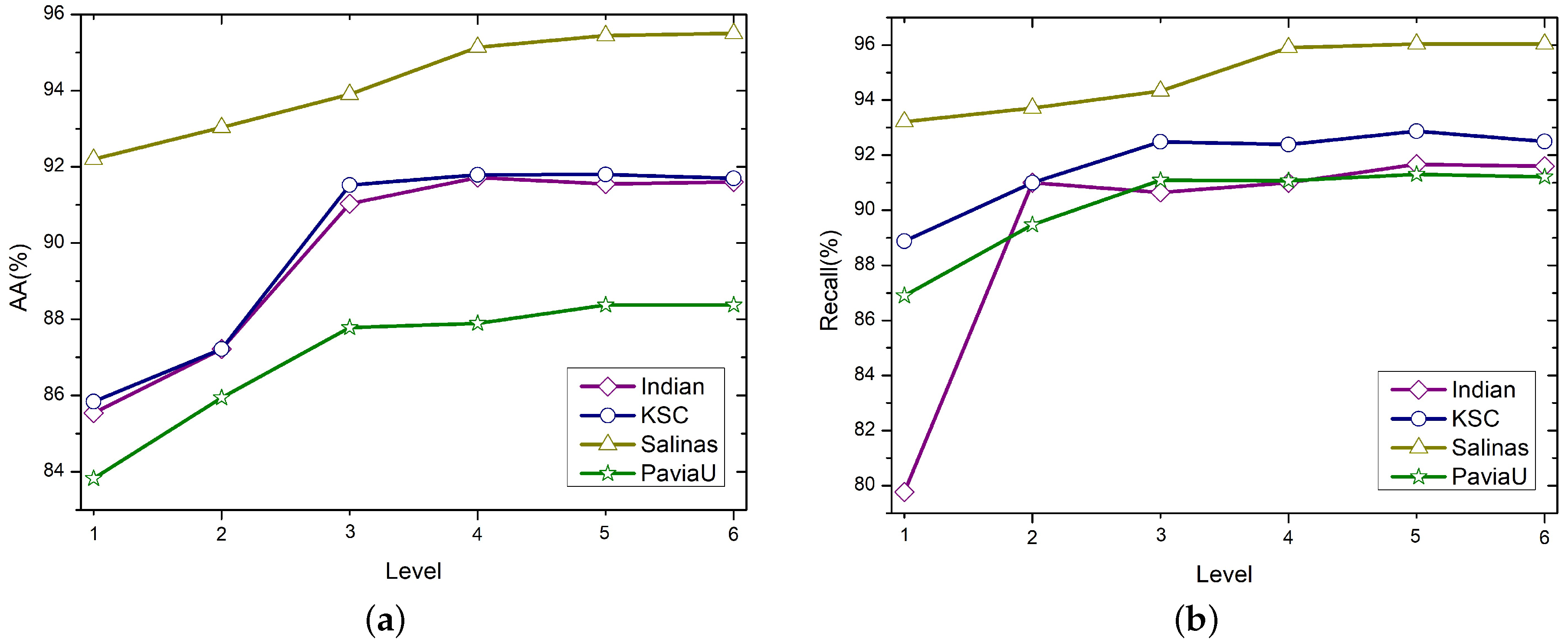
4.5.1. Influence of Level

In order to study the influence of level on SMOTE-WDRoF, we present in Figure 7 the evolution of the AA and Recall on Indian Pines AVRIS, KSC, Salinas and University of Pavia ROSIS. Similar to the traditional depth model, the deep forest structure of SMOTE-WDRoF is of great significance to improve the classification performance. When the output of each level is used as the feature and stacked with the original feature as the input of the next level, the sample weights are adjusted accordingly. Consequently, the classification accuracy is enhanced with the growth of the level. As can be seen from Figure 7a, AA of four hyperspectral datasets is increased significantly when the level increased from 1 to 3. When the level is 4, the growth rate of AA slowed down gradually. And when the level number exceeds 5, the AA of the four datasets reaches a stable value. For Indian Pines AVRIS, KSC, Salinas and University of Pavia ROSIS, the stable values are 91.55%, 91.87%, 95.44% and 88.37% respectively. The evolution of the Recall on four hyperspectral datasets is shown in Figure 7b. It can be observed that at first recall is increased greatly. With the increase in levels, the recall turns to a relatively stable value. When the level is set as 5, the stable values are 91.67%, 92.40%, 96.05% and 91.28% respectively on Indian Pines AVRIS, KSC, Salinas and University of Pavia ROSIS. These results demonstrate that when there are too many levels in the proposed model, the output of the last several levels cannot afford helpful information for classification anymore. Therefore, statistically better performance can be achieved when L is equal to 5. And in other experiments, the level is set as 5.

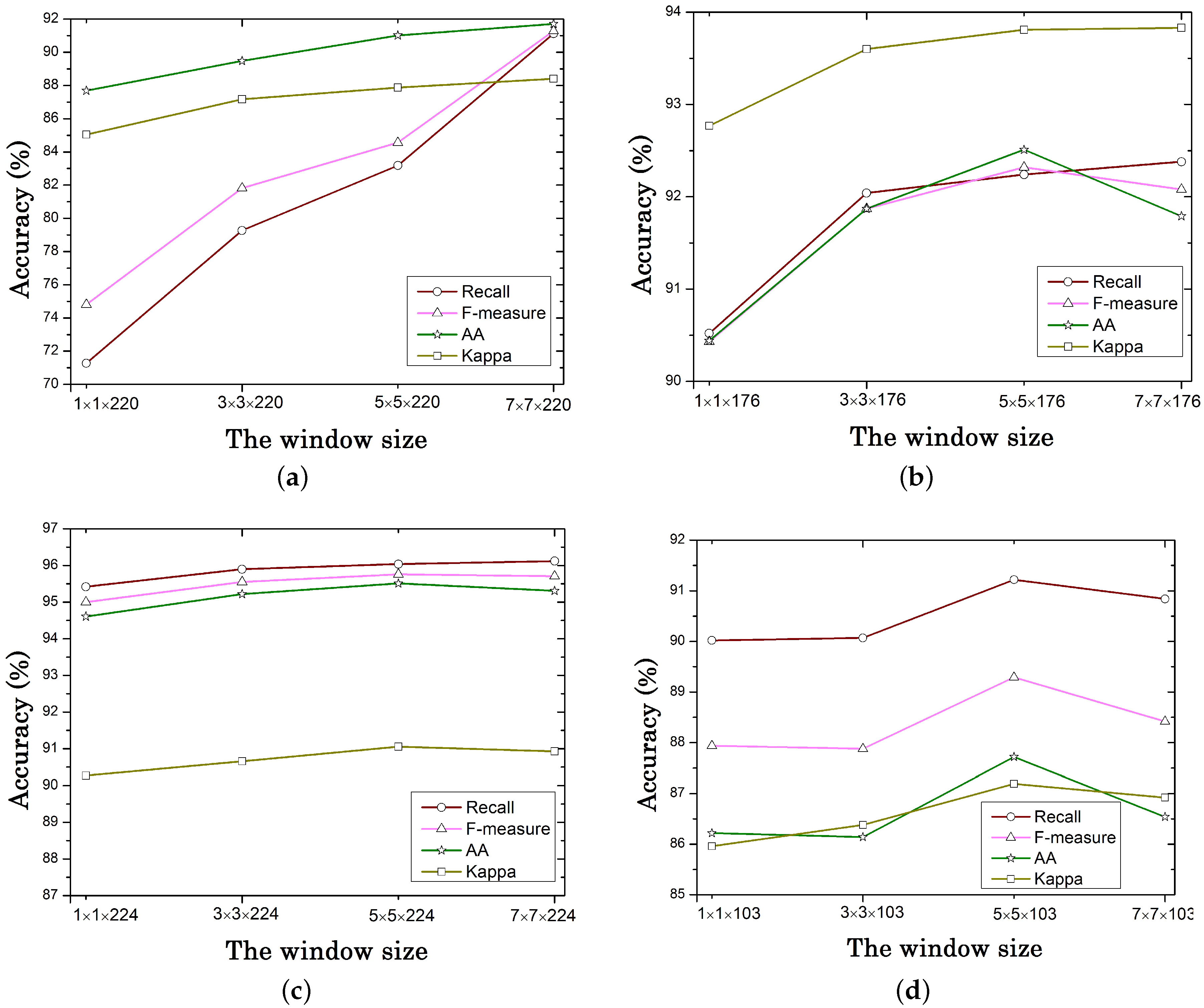
4.5.2. Influence of the Window Size

Due to the spatial homogeneity of hyperspectral images, neighboring samples are likely to belong to the same class. Consequently, neighboring pixels are introduced to be the local spatial information by a sliding window in SMOTE-WDRoF. To study the influence of window size on classification accuracies, we vary this parameter from 1 × 1 × D to 7 × 7 × D for four hyperspectral datasets to introduce different numbers of spatial neighbor pixels. D represents the number of bands for hyperspectral data. For Indian Pines AVRIS, KSC, Salinas and University of Pavia ROSIS, D are 220, 176, 224 and 103 respectively. The results with different window sizes are shown in Figure 8. While the window size increases, the classification accuracy also presents an upward trend. More specifically, for Indian Pines AVRIS, AA, Recall, F-measure and Kappa increase from 87.69%, 71.27%, 74.81% and 85.05% to 91.71%, 91.12%, 91.29% and 88.41% respectively when the size of window is changed from 1 × 1 × 1 × 220 to 7 × 7 × 220 . And the highest precision of Indian Pines AVRIS is obtained at 7 × 7 × 220 . For KSC, the three indexes, Recall, AA, and F-measure, reach the highest precision at 7 × 7 × 176 . Besides, the value of Kappa first rises and then falls, and it achieves the highest value at 5 × 5 × 176 . For Salinas, the high precision is obtained at 5 × 5 × 224 , and then the precision almost no longer increases with the expansion of the window size. In addition, SMOTE-WDRoF with a window size of 5 × 5 × 103 delivers the best performance for University of Pavia ROSIS. This phenomenon is not surprising. More useful spatial information can be introduced by a relatively large window, which is beneficial to improve classification performance. However, if the window size is too large, samples that do not belong to the same class as the central pixel will be extracted, which will result in the decreased accuracy.

5. Conclusions

In this paper, the SMOTE-Based Weighted Deep Rotation Forest(SMOTE-WDRoF) algorithm is proposed for the imbalanced hyperspectral data classification. First of all, the local spatial structure of samples is extract to enrich the data information, and the balanced datasets are built by SMOTE. Second, RoF and multi-layer cascade RF form the WDRoF model which uses the output probability of each layer as a supplement feature of the next layer and updates the sample weights adaptively to improve classification performance. The proposed method is validated on four public hyperspectral image datasets. Compared with the traditional deep learning models, SMOTE-WDRoF consumes much less training time. Experimental results show that the proposed SMOTE-WDRoF is effective for dealing with multi-class imbalanced data and significantly outperforms SVM, RF, RoF, SMOTE-RoF, CNN, and RBDF and Besides, the parameter analysis has also been implemented and the results have demonstrated the advantages of our algorithm in terms of accuracy and robustness.

Author Contributions

Y.Q. and W.F. conceived and designed the experiments; X.Z. performed the experiments and wrote the paper. J.C.-W.C. and Q.L. revised the paper. M.X. edited the manuscript. All authors have read and agreed to the published version of the manuscript.

Funding

This research was funded by the National Natural Science Foundation of China (61772397, 12005169), National Key R&D Program of China (2016YFE0200400), the Open Research Fund of Key Laboratory of Digital Earth Science (2019LDE005), science and technology innovation team of Shaanxi Province (2019TD-002), Fundamental Research Funds for the Central Universities (XJS200205), and the Fundamental Research Funds for the Central Universities and the Innovation Fund of Xidian University.

Institutional Review Board Statement

Not applicable.

Informed Consent Statement

Not applicable.

Data Availability Statement

Publicly available datasets were analyzed in this study. This data can be found here: [http://www.ehu.eus/ccwintco/index.php?title=Hyperspectral_Remote_Sensing_Scenes].

Acknowledgments

This work is supported by the National Natural Science Foundation of China (61772397, 12005169), National Key R&D Program of China (2016YFE0200400), the Open Research Fund of Key Laboratory of Digital Earth Science (2019LDE005), science and technology innovation team of Shaanxi Province (2019TD-002), Fundamental Research Funds for the Central Universities (XJS200205), and the Fundamental Research Funds for the Central Universities and the Innovation Fund of Xidian University.

Conflicts of Interest

The authors declare no conflict of interest.

References

  1. Zhang, M.; Li, W.; Du, Q. Diverse Region-Based CNN for Hyperspectral Image Classification. IEEE Trans. Image Process. 2018, 27, 2623–2634. [Google Scholar] [CrossRef] [PubMed]
  2. Landgrebe, D. Hyperspectral image data analysis. IEEE Signal Process. Mag. 2002, 19, 17–28. [Google Scholar] [CrossRef]
  3. Li, H.; Song, Y.; Chen, C.P. Hyperspectral Image Classification Based on Multiscale Spatial Information Fusion. IEEE Trans. Geosci. Remote Sens. 2017, 55, 5302–5312. [Google Scholar] [CrossRef]
  4. Zheng, X.; Yuan, Y.; Lu, X. Dimensionality Reduction by Spatial–Spectral Preservation in Selected Bands. IEEE Trans. Geosci. Remote Sens. 2017, 55, 5185–5197. [Google Scholar] [CrossRef]
  5. Lin, L.; Song, X. Using CNN to Classify Hyperspectral Data Based on Spatial-spectral Information. Adv. Intell. Inf. Hiding Multimed. Signal Process. 2017, 64, 61–68. [Google Scholar]
  6. Yuan, Y.; Feng, Y.; Lu, X. Projection-Based NMF for Hyperspectral Unmixing. IEEE J. Sel. Top. Appl. Earth Obs. Remote Sens. 2015, 8, 2632–2643. [Google Scholar] [CrossRef]
  7. Feng, W.; Huang, W.; Bao, W. Imbalanced Hyperspectral Image Classification with an Adaptive Ensemble Method Based on SMOTE and Rotation Forest with Differentiated Sampling Rates. IEEE Geosci. Remote Sens. Lett. 2019, 16, 1879–1883. [Google Scholar] [CrossRef]
  8. Quan, Y.; Zhong, X.; Feng, W.; Dauphin, G.; Xing, M. A Novel Feature Extension Method for the Forest Disaster Monitoring Using Multispectral Data. Remote Sens. 2020, 12, 2261. [Google Scholar] [CrossRef]
  9. Jiang, M.; Fang, Y.; Su, Y.; Cai, G.; Han, G. Random Subspace Ensemble With Enhanced Feature for Hyperspectral Image Classification. IEEE Geosci. Remote Sens. Lett. 2019, 17, 1373–1377. [Google Scholar] [CrossRef]
  10. Zhao, Q.; Jia, S.; Li, Y. Hyperspectral remote sensing image classification based on tighter random projection with minimal intra-class variance algorithm. Pattern Recognit. 2020, 111, 107635. [Google Scholar] [CrossRef]
  11. Shi, T.; Liu, H.; Chen, Y.; Wang, J.; Wu, G. Estimation of arsenic in agricultural soils using hyperspectral vegetation indices of rice. J. Hazard. Mater. 2016, 308, 243–252. [Google Scholar] [CrossRef] [PubMed]
  12. Obermeier, W.A.; Lehnert, L.W.; Pohl, M.J.; Gianonni, S.M.; Silva, B.; Seibert, R.; Laser, H.; Moser, G.; Müller, C.; Luterbacher, J.; et al. Grassland ecosystem services in a changing environment: The potential of hyperspectral monitoring. Remote Sens. Environ. 2019, 232, 111273. [Google Scholar] [CrossRef]
  13. Zhang, M.; English, D.; Hu, C.; Carlson, P.; Muller-Karger, F.E.; Toro-Farmer, G.; Herwitz, S.R. Short-term changes of remote sensing reflectancein a shallow-water environment: Observations from repeated airborne hyperspectral measurements. Int. J. Remote Sens. 2016, 37, 1620–1638. [Google Scholar] [CrossRef]
  14. Li, Q.; Feng, W.; Quan, Y.H. Trend and forecasting of the COVID-19 outbreak in China. J. Infect. 2020, 80, 469–496. [Google Scholar]
  15. Pontius, J.; Hanavan, R.P.; Hallett, R.A.; Cook, B.D.; Corp, L.A. High spatial resolution spectral unmixing for mapping ash species across a complex urban environment. Remote Sens. Environ. 2017, 199, 360–369. [Google Scholar] [CrossRef]
  16. Richards, J.A.; Jia, X. Using Suitable Neighbors to Augment the Training Set in Hyperspectral Maximum Likelihood Classification. IEEE Geosci. Remote Sens. Lett. 2008, 5, 774–777. [Google Scholar] [CrossRef]
  17. Guo, X.; Huang, X.; Zhang, L.; Zhang, L.; Plaza, A.; Benediktsson, J.A. Support Tensor Machines for Classification of Hyperspectral Remote Sensing Imagery. IEEE Trans. Geosci. Remote Sens. 2016, 54, 3248–3264. [Google Scholar] [CrossRef]
  18. Meher, S.K. Knowledge-Encoded Granular Neural Networks for Hyperspectral Remote Sensing Image Classification. IEEE J. Sel. Top. Appl. Earth Obs. Remote Sens. 2015, 8, 2439–2446. [Google Scholar] [CrossRef]
  19. Li, J.; Du, Q.; Li, Y.; Li, W. Hyperspectral Image Classification with Imbalanced Data Based on Orthogonal Complement Subspace Projection. IEEE Trans. Geosci. Remote Sens. 2018, 56, 3838–3851. [Google Scholar] [CrossRef]
  20. Mi, Y. Imbalanced Classification Based on Active Learning SMOTE. Res. J. Appl. Eng. Technol. 2013, 5, 944–949. [Google Scholar] [CrossRef]
  21. Taherkhani, A.; Cosma, G.; McGinnity, T.M. AdaBoost-CNN: An Adaptive Boosting algorithm for Convolutional Neural Networks to classify Multi-Class Imbalanced datasets using Transfer Learning. Neurocomputing 2020, 404, 351–366. [Google Scholar] [CrossRef]
  22. Zhang, X.; Zhuang, Y.; Wang, W.; Pedrycz, W. Transfer Boosting With Synthetic Instances for Class Imbalanced Object Recognition. IEEE Trans. Cybern. 2016, 48, 357–370. [Google Scholar] [CrossRef] [PubMed]
  23. Anand, A.; Pugalenthi, G.; Fogel, G.B.; Suganthan, P.N. An approach for classification of highly imbalanced data using weighting and undersampling. Amino Acids 2010, 39, 1385–1391. [Google Scholar] [CrossRef] [PubMed]
  24. Lin, M.; Tang, K.; Yao, X. Dynamic Sampling Approach to Training Neural Networks for Multiclass Imbalance Classification. IEEE Trans. Neural Netw. Learn. Syst. 2013, 24, 647–660. [Google Scholar]
  25. Feng, W.; Huang, W.; Ren, J. Class Imbalance Ensemble Learning Based on the Margin Theory. Appl. Sci. 2018, 8, 815. [Google Scholar] [CrossRef] [Green Version]
  26. Feng, W.; Dauphin, G.; Huang, W.; Quan, Y.; Liao, W. New Margin-Based Subsampling Iterative Technique In Modified Random Forests for Classification. Knowl. Based Syst. 2019, 182, 104845. [Google Scholar] [CrossRef]
  27. Feng, W.; Bao, W. Weight-Based Rotation Forest for Hyperspectral Image Classification. IEEE Geosci. Remote Sens. Lett. 2017, 14, 2167–2171. [Google Scholar] [CrossRef]
  28. Castellanos, F.J.; Valero-Mas, J.J.; Calvo-Zaragoza, J.; Rico-Juan, J.R. Oversampling imbalanced data in the string space. Pattern Recognit. Lett. 2018, 103, 32–38. [Google Scholar] [CrossRef] [Green Version]
  29. Chawla, N.V.; Bowyer, K.W.; Hall, L.O.; Kegelmeyer, W.P. SMOTE: Synthetic Minority Over-sampling Technique. J. Artif. Intell. Res. 2002, 16, 321–357. [Google Scholar] [CrossRef]
  30. Blaszczynski, J.; Stefanowski, J. Neighbourhood sampling in bagging for imbalanced data. Neurocomputing 2015, 150, 529–542. [Google Scholar] [CrossRef]
  31. Qi, K.; Yang, H.; Hu, Q.; Yang, D. A new adaptive weighted imbalanced data classifier via improved support vector machines with high-dimension nature. Knowl. Based Syst. 2019, 185, 104933. [Google Scholar] [CrossRef]
  32. Zhou, Z.H.; Liu, X.Y. Training cost-sensitive neural networks with methods addressing the class imbalance problem. IEEE Trans. Knowl. Data Eng. 2006, 18, 63–77. [Google Scholar] [CrossRef]
  33. Datta, A.; Ghosh, S.; Ghosh, A. Combination of Clustering and Ranking Techniques for Unsupervised Band Selection of Hyperspectral Images. IEEE J. Sel. Top. Appl. Earth Obs. Remote Sens. 2015, 8, 2814–2823. [Google Scholar] [CrossRef]
  34. Galar, M. A Review on Ensembles for the Class Imbalance Problem: Bagging-, Boosting-, and Hybrid-Based Approaches. IEEE Trans. Syst. Man Cybern. Part C Appl. Rev. 2012, 42, 463–484. [Google Scholar] [CrossRef]
  35. Ng, W.W.Y.; Hu, J.; Yeung, D.S.; Yin, S.; Roli, F. Diversified Sensitivity-Based Undersampling for Imbalance Classification Problems. IEEE Trans. Cybern. 2017, 45, 2402–2412. [Google Scholar] [CrossRef]
  36. Ming, G.; Xia, H.; Sheng, C.; Harris, C.J. A combined SMOTE and PSO based RBF classifier for two-class imbalanced problems. Neurocomputing 2011, 74, 3456–3466. [Google Scholar]
  37. Liu, X.Y.; Wu, J.; Zhou, Z.H. Exploratory undersampling for class-imbalance learning. IEEE Trans. Syst. Man Cybern. Part B Cybern. 2008, 39, 539–550. [Google Scholar]
  38. Barandela, R.; Valdovinos, R.M.; Sánchez Garreta, J.S.; Ferri, F.J. The Imbalance Training Sample Problem: Under or over Sampling. In Joint IAPR International Workshops on Statistical Techniques in Pattern Recognition (SPR) and Structural and Syntactic Pattern Recognition (SSPR); Springer: Berlin/Heidelberg, Germany, 2004; Volume 3138, pp. 806–814. [Google Scholar]
  39. Liu, B.; Tsoumakas, G. Dealing with class imbalance in classifier chains via random undersampling. Knowl. Based Syst. 2020, 192, 105292.1–105292.13. [Google Scholar] [CrossRef]
  40. Akkasi, A.; Varolu, E.; Dimililer, N. Balanced undersampling: A novel sentence-based undersampling method to improve recognition of named entities in chemical and biomedical text. Appl. Intell. 2017, 48, 1–14. [Google Scholar] [CrossRef]
  41. Kang, Q.; Chen, X.S.; Li, S.S.; Zhou, M.C. A Noise-Filtered Under-Sampling Scheme for Imbalanced Classification. IEEE Trans. Cybern. 2017, 47, 4263–4274. [Google Scholar] [CrossRef]
  42. Ng, W.W.Y.; Xu, S.; Zhang, J.; Tian, X.; Rong, T.; Kwong, S. Hashing-Based Undersampling Ensemble for Imbalanced Pattern Classification Problems. IEEE Trans. Cybern. 2020, 1–11. [Google Scholar] [CrossRef] [PubMed]
  43. De Morais, R.F.A.B.; Vasconcelos, G.C. Boosting the Performance of Over-Sampling Algorithms through Under-Sampling the Minority Class. Neurocomputing 2019, 343, 3–18. [Google Scholar] [CrossRef]
  44. Batista, G.E.A.P.A.; Prati, R.C.; Monard, M.C. A study of the behavior of several methods for balancing machine learning training data. ACM SIGKDD Explor. Newsl. 2004, 6, 20–29. [Google Scholar] [CrossRef]
  45. Prusty, M.R.; Jayanthi, T.; Velusamy, K. Weighted-SMOTE: A modification to SMOTE for event classification in sodium cooled fast reactors. Prog. Nucl. Energy 2017, 100, 355–364. [Google Scholar] [CrossRef]
  46. Douzas, G.; Bacao, F.; Fonseca, J.; Khudinyan, M. Imbalanced Learning in Land Cover Classification: Improving Minority Classes’ Prediction Accuracy Using the Geometric SMOTE Algorithm. Remote Sens. 2019, 11, 3040. [Google Scholar] [CrossRef] [Green Version]
  47. Sun, J.; Lang, J.; Fujita, H.; Li, H. Imbalanced enterprise credit evaluation with DTE-SBD: Decision tree ensemble based on SMOTE and bagging with differentiated sampling rates. Inf. Sci. 2018, 425, 76–91. [Google Scholar] [CrossRef]
  48. Ertekin, S.; Huang, J.; Bottou, L.; Giles, C.L. Learning on the border: Active learning in imbalanced data classification. In Proceedings of the Sixteenth ACM Conference on Information & Knowledge Management, Lisbon, Portugal, 6–10 November 2007; Association for Computing Machinery: New York, NY, USA, 2007; pp. 127–136. [Google Scholar]
  49. Sun, Y.; Kamel, M.S.; Wong, A.K.C.; Wang, Y. Cost-sensitive boosting for classification of imbalanced data. Pattern Recognit. 2007, 40, 3358–3378. [Google Scholar] [CrossRef]
  50. He, H.; Garcia, E.A. Learning from Imbalanced Data. IEEE Trans. Knowl. Data Eng. 2009, 21, 1263–1284. [Google Scholar]
  51. Ding, S.; Mirza, B.; Lin, Z.; Cao, J.; Sepulveda, J. Kernel based online learning for imbalance multiclass classification. Neurocomputing 2017, 277, 139–148. [Google Scholar] [CrossRef]
  52. Yu, H.; Yang, X.; Zheng, S.; Sun, C. Active Learning From Imbalanced Data: A Solution of Online Weighted Extreme Learning Machine. IEEE Trans. Neural Netw. Learn. Syst. 2019, 30, 1088–1103. [Google Scholar] [CrossRef]
  53. Zhang, H.; Liu, W.; Shan, J.; Liu, Q. Online Active Learning Paired Ensemble for Concept Drift and Class Imbalance. IEEE Access 2018, 6, 73815–73828. [Google Scholar] [CrossRef]
  54. Sun, T.; Jiao, L.; Feng, J.; Liu, F.; Zhang, X. Imbalanced Hyperspectral Image Classification Based on Maximum Margin. IEEE Geosci. Remote Sens. Lett. 2015, 12, 522–526. [Google Scholar] [CrossRef]
  55. Feng, W.; Dauphin, G.; Huang, W.; Quan, Y.; Bao, W.; Wu, M.; Li, Q. Dynamic Synthetic Minority Over-Sampling Technique-Based Rotation Forest for the Classification of Imbalanced Hyperspectral Data. IEEE J. Sel. Top. Appl. Earth Obs. Remote Sens. 2019, 12, 2159–2169. [Google Scholar] [CrossRef]
  56. Vapnik, V.N. The Nature of Statistical Learning Theory; Springer: Berlin/Heidelberg, Germany, 2013. [Google Scholar]
  57. Japkowicz, N.; Stephen, S. The class imbalance problem: A systematic study. Intell. Data Anal. 2002, 6, 429–449. [Google Scholar] [CrossRef]
  58. Akbani, R.; Kwek, S.S.; Japkowicz, N. Applying Support Vector Machines to Imbalanced Datasets; Springer: Berlin/Heidelberg, Germany, 2004; pp. 39–50. [Google Scholar]
  59. Kang, P.; Cho, S. EUS SVMs: Ensemble of Under-Sampled SVMs for Data Imbalance Problems. In Proceedings of the International Conference on Neural Information Processing; Springer: Berlin/Heidelberg, Germany, 2006; pp. 837–846. [Google Scholar]
  60. Qi, W.; Luo, Z.H.; Huang, J.C.; Feng, Y.H.; Zhong, L. A Novel Ensemble Method for Imbalanced Data Learning: Bagging of Extrapolation-SMOTE SVM. Comput. Intell. Neurosci. 2017, 2017, 1827016. [Google Scholar]
  61. Ying, L.; Haokui, Z.; Qiang, S. Spectral–Spatial Classification of Hyperspectral Imagery with 3D Convolutional Neural Network. Remote Sens. 2017, 9, 67. [Google Scholar] [CrossRef] [Green Version]
  62. Sellami, A.; Abbes, A.B.; Barra, V.; Farah, I.R. Fused 3-D spectral-spatial deep neural networks and spectral clustering for hyperspectral image classification. Pattern Recognit. Lett. 2020, 138, 594–600. [Google Scholar] [CrossRef]
  63. Li, S.; Song, W.; Fang, L.; Chen, Y.; Ghamisi, P.; Benediktsson, J.A. Deep Learning for Hyperspectral Image Classification: An Overview. IEEE Trans. Geosci. Remote Sens. 2019, 57, 6690–6709. [Google Scholar] [CrossRef] [Green Version]
  64. Chen, Y.; Wang, Y.; Gu, Y.; He, X.; Ghamisi, P.; Jia, X. Deep Learning Ensemble for Hyperspectral Image Classification. IEEE J. Sel. Top. Appl. Earth Obs. Remote Sens. 2019, 12, 1882–1897. [Google Scholar] [CrossRef]
  65. Li, S.; Song, W.; Qin, H.; Hao, A. Deep variance network: An iterative, improved CNN framework for unbalanced training datasets. Pattern Recognit. J. Pattern Recognit. Soc. 2018, 81, 294–308. [Google Scholar] [CrossRef]
  66. Buda, M.; Maki, A.; Mazurowski, M.A. A systematic study of the class imbalance problem in convolutional neural networks. Neural Netw. Off. J. Int. Neural Netw. Soc. 2018, 106, 249–259. [Google Scholar] [CrossRef] [PubMed] [Green Version]
  67. Cao, X.; Wen, L.; Ge, Y.; Zhao, J.; Jiao, L. Rotation-Based Deep Forest for Hyperspectral Imagery Classification. IEEE Geosci. Remote Sens. Lett. 2019, 16, 1105–1109. [Google Scholar] [CrossRef]
  68. Breiman, L. Bagging Predictors. Mach. Learn. 1996, 24, 123–140. [Google Scholar] [CrossRef] [Green Version]
  69. Breiman, L. Random Forests. Mach. Learn. 2001, 45, 5–32. [Google Scholar] [CrossRef] [Green Version]
  70. Rodriguez, J.J.; Kuncheva, L.I.; Alonso, C.J. Rotation Forest: A New Classifier Ensemble Method. IEEE Trans. Pattern Anal. Mach. Intell. 2006, 28, 1619–1630. [Google Scholar] [CrossRef] [PubMed]
  71. Hu, W.; Huang, Y.; Li, W.; Zhang, F.; Li, H. Deep Convolutional Neural Networks for Hyperspectral Image Classification. J. Sens. 2015, 2015, 1–12. [Google Scholar] [CrossRef] [Green Version]
  72. Fernández, A.; López, V.; Galar, M.; del Jesus, M.J.; Herrera, F. Analysing the classification of imbalanced data-sets with multiple classes: Binarization techniques and ad-hoc approaches. Knowl. Based Syst. 2013, 42, 97–110. [Google Scholar] [CrossRef]
  73. Sáez, J.A.; Krawczyk, B.; Woźniak, M. Analyzing the oversampling of different classes and types of examples in multi-class imbalanced datasets. Pattern Recognit. 2016, 57, 164–178. [Google Scholar] [CrossRef]
  74. Xu, X.; Chen, W.; Sun, Y. Over-sampling algorithm for imbalanced data classification. J. Syst. Eng. Electron. 2019, 30, 1182–1191. [Google Scholar] [CrossRef]
  75. Yan, Y.; Liu, R.; Ding, Z.; Du, X.; Chen, J.; Zhang, Y. A Parameter-free Cleaning Method for SMOTE in Imbalanced Classification. IEEE Access 2019, 7, 23537–23548. [Google Scholar] [CrossRef]
Figure 1. The Flow Chart of Spatial Information Extraction and Balanced Datasets Generation.
Remotesensing 13 00464 g001
Figure 2. The Flow Chart of WDRoF.
Remotesensing 13 00464 g002
Figure 3. Ground truth (GT) and classification maps of SVM, RF, RoF, CNN, SMOTE-RoF, RBDF as well as the proposed SMOTE-WDRoF method on the hyperspectral data Indian Pines AVRIS. (a) GT. (b) SVM. (c) RF. (d) RoF. (e) SMOTE-RoF. (f) CNN. (g) RBDF. (h) SMOTE-WDRoF.
Remotesensing 13 00464 g003
Figure 4. Ground truth (GT) and classification maps of SVM, RF, RoF, CNN, SMOTE-RoF, RBDF as well as the proposed SMOTE-WDRoF method on the hyperspectral data KSC. (a) GT. (b) SVM. (c) RF. (d) RoF. (e) SMOTE-RoF. (f) CNN. (g) RBDF. (h) SMOTE-WDRoF.
Remotesensing 13 00464 g004
Figure 5. Ground truth (GT) and classification maps of SVM, RF, RoF, CNN, SMOTE-RoF, RBDF as well as the proposed SMOTE-WDRoF method on the hyperspectral data Salinas. (a) GT. (b) SVM. (c) RF. (d) RoF. (e) SMOTE-RoF. (f) CNN. (g) RBDF. (h) SMOTE-WDRoF.
Remotesensing 13 00464 g005aRemotesensing 13 00464 g005b
Figure 6. Ground truth (GT) and classification maps of SVM, RF, RoF, CNN, SMOTE-RoF, RBDF as well as the proposed SMOTE-WDRoF method on the hyperspectral data the University of Pavia ROSIS. (a) GT. (b) SVM. (c) RF. (d) RoF. (e) SMOTE-RoF. (f) CNN. (g) RBDF. (h) SMOTE-WDRoF.
Remotesensing 13 00464 g006
Figure 7. (a) Evolution of the AA according to level. (b) Evolution of the Recall according to level.
Remotesensing 13 00464 g007
Figure 8. Recall, AA, F-measure and Kappa of SMOTE-WDRoF with different window sizes on four hyperspectral image datasets. (a) Indian Pines AVRIS, (b) KSC, (c) Salinas and (d) the University of Pavia ROSIS.
Remotesensing 13 00464 g008
Table 1. Data information of Indian Pines AVRIS, Salinas, KSC and University of Pavia ROSIS.
The DatasetIndian Pines AVRISSalinas
Class No.TrainTestClass No.TrainTest
1Alfalfa2323Brocoli_green_weeds_11001909
2Corn-notill4281000Brocoli_green_weeds_21863540
3Corn-mintill249581cFallow981878
4Corn71166cFallow_rough_plow681325
5Grass-pasture144339Fallow_smooth1332545
6Corn-trees219511Stubble1973762
7Corn-pasture-mowed1414Celery1783401
8Hay-windrowed143335Grapes_untrained56310,708
9Oats1010Soil_vinyard_develop3105893
10Soybeans-notill291681Corn_senesced_green_weeds1633115
11Soybeans-mintill7361719Lettuce_romaine_4wk531015
12Soybeans-clean177416Lettuce_romaine_5wk961831
13Wheat61144Lettuce_romaine_6wk45871
14Woods379886Lettuce_romaine_7wk531017
15Buildings-Grass-Trees-Drivers115271Vinyard_untrained3636905
16Stone-steel-Towers4647Vinyard_vertical_trellis901717
Total 31067143 269751,432
The DatasetKSCUniversity of Pavia ROSIS
Class No.TrainTestClass No.TrainTest
1Scrub229532Asphalt3316300
2Willow swamp73170Meadows93217,717
3Cabbage palm ham80179Gravel1041995
4Cabbage palm/oak ham76176Trees1532911
5Slash pine49112Painted metal sheets671278
6Oak/broadleaf ham69160Bare Soil2514778
7Hardwood swamp3273Bitumen661264
8Graminoid marsh130301Self-Blocking Bricks1843498
9Spartina marsh157363Shadows47900
10Cattail marsh122282
11Salt marsh126293
12Mud flats151352
13Water279648
Total 15733635 213540,641
Table 2. Classification results (%) of the Indian pines AVRIS image, respectively obtained by SVM, RF, RoF, SMOTE-RoF, CNN, RBDF and the proposed SMOTE-WDRoF in the case of the imbalance ratio of 73.6.
IR: 73.6SVMRFRoFSMOTE-RoFCNNRBDFSMOTE-WDRoF
1 67.70 ± 6.36 85.88 ± 8.14 67.97 ± 9.16 66.86 ± 8.69 70.37 ± 16.15 83.46 ± 2.46 96.88 ± 2.28
2 75.48 ± 1.55 73.78 ± 0.94 72.49 ± 0.82 71.84 ± 0.98 83.60 ± 11.93 83.39 ± 0.46 86.46 ± 0.61
3 70.27 ± 1.06 77.12 ± 2.10 70.32 ± 0.97 72.07 ± 1.41 80.45 ± 6.33 85.69 ± 0.42 82.97 ± 0.64
4 67.79 ± 3.93 60.64 ± 3.12 61.11 ± 2.20 62.58 ± 2.96 64.50 ± 11.29 78.65 ± 1.52 81.18 ± 0.49
5 91.15 ± 1.58 92.97 ± 0.57 91.61 ± 1.20 87.89 ± 0.84 88.33 ± 6.12 95.72 ± 0.28 94.30 ± 0.46
6 92.88 ± 0.97 88.05 ± 0.75 92.09 ± 0.63 91.52 ± 1.42 96.35 ± 3.53 95.16 ± 0.36 96.77 ± 0.08
7 85.36 ± 5.16 93.00 ± 10.95 74.91 ± 10.83 93.71 ± 10.05 81.25 ± 8.37 93.12 ± 1.77 93.29 ± 4.19
8 98.56 ± 0.90 95.71 ± 0.82 98.78 ± 0.36 98.25 ± 0.39 99.39 ± 0.66 97.95 ± 0.27 98.67 ± 0.06
9 43.09 ± 6.20 73.57 ± 10.28 79.64 ± 16.58 57.75 ± 12.67 47.06 ± 6.56 81.89 ± 5.93 96.39 ± 1.33
10 76.41 ± 0.90 75.85 ± 1.70 79.13 ± 0.54 78.09 ± 1.51 78.17 ± 7.79 84.89 ± 0.46 84.20 ± 0.34
11 78.89 ± 0.43 76.07 ± 0.63 81.42 ± 0.69 83.03 ± 3.23 78.17 ± 4.26 84.28 ± 0.32 90.54 ± 0.22
12 81.32 ± 1.94 73.21 ± 1.01 77.49 ± 2.78 77.39 ± 3.80 80.25 ± 7.90 84.54 ± 0.30 84.84 ± 0.40
13 94.53 ± 3.06 91.93 ± 1.78 94.34 ± 2.84 87.68 ± 12.42 95.30 ± 2.29 95.26 ± 0.40 98.95 ± 0.15
14 93.96 ± 1.37 91.16 ± 0.75 92.16 ± 0.70 92.55 ± 0.90 97.15 ± 2.69 95.99 ± 0.11 97.51 ± 0.13
15 72.87 ± 2.73 76.75 ± 1.40 76.28 ± 2.93 75.57 ± 2.16 72.52 ± 12.45 86.23 ± 0.51 82.35 ± 0.32
16 95.71 ± 3.26 99.00 ± 2.23 98.64 ± 1.23 97.36 ± 0.95 93.75 ± 1.81 96.84 ± 0.48 99.48 ± 0.56
AA (%) 80.37 ± 0.54 82.80 ± 0.40 81.77 ± 1.26 80.88 ± 1.24 81.66 ± 0.91 88.94 ± 0.44 91.55 ± 0.44
Recall (%) 81.71 ± 1.77 75.78 ± 1.62 81.42 ± 0.82 81.35 ± 2.20 89.77 ± 0.71 87.72 ± 0.20 91.67 ± 0.40
F-measure (%) 80.58 ± 0.90 78.45 ± 1.31 81.26 ± 1.04 81.05 ± 1.40 85.46 ± 0.64 88.21 ± 0.29 91.51 ± 0.34
Kappa (%) 79.26 ± 0.20 77.62 ± 0.16 79.33 ± 0.22 79.57 ± 0.30 84.88 ± 2.47 86.35 ± 0.18 88.64 ± 0.18
Table 3. Classification results (%) of the KSC image, respectively obtained by SVM, RF, RoF, SMOTE-RoF, CNN, RBDF and the proposed SMOTE-WDRoF in the case of the imbalance ratio of 8.71.
IR: 8.71SVMRFRoFSMOTE-RoFCNNRBDFSMOTE-WDRoF
1 74.23 ± 1.20 91.96 ± 0.62 89.89 ± 0.99 93.12 ± 1.26 85.57 ± 15.13 90.37 ± 1.25 97.25 ± 0.26
2 70.96 ± 1.91 80.20 ± 1.99 90.17 ± 1.75 88.03 ± 1.59 80.46 ± 6.76 86.35 ± 3.42 93.20 ± 1.12
3 60.86 ± 10.39 88.66 ± 0.73 89.21 ± 1.00 86.29 ± 2.24 73.30 ± 19.32 87.76 ± 4.19 91.63 ± 1.29
4 35.80 ± 4.34 60.49 ± 0.50 62.58 ± 2.14 66.53 ± 1.98 61.40 ± 19.21 72.92 ± 2.42 80.45 ± 2.06
5 64.98 ± 37.91 79.39 ± 3.99 71.26 ± 6.81 72.58 ± 4.36 79.45 ± 11.57 75.20 ± 4.16 82.36 ± 3.31
6 55.29 ± 9.64 70.10 ± 4.24 66.44 ± 4.32 66.17 ± 2.92 65.22 ± 37.52 78.91 ± 3.19 79.50 ± 0.71
7 0.00 ± 0.00 73.79 ± 1.87 80.70 ± 2.10 85.09 ± 3.89 75.00 ± 10.62 86.76 ± 3.04 90.19 ± 2.48
8 65.71 ± 4.01 85.72 ± 1.43 86.74 ± 1.84 85.07 ± 1.42 79.73 ± 4.96 86.64 ± 3.24 90.70 ± 1.37
9 71.79 ± 1.84 89.97 ± 0.61 91.75 ± 0.95 94.86 ± 0.50 82.08 ± 1.79 91.40 ± 0.36 94.88 ± 0.69
10 99.12 ± 1.09 96.41 ± 1.20 98.77 ± 0.31 98.28 ± 0.67 98.13 ± 5.91 97.27 ± 1.52 98.43 ± 0.35
11 95.15 ± 1.61 99.04 ± 0.28 99.12 ± 0.83 97.52 ± 0.78 98.25 ± 0.33 98.64 ± 0.57 99.84 ± 0.09
12 76.74 ± 1.07 93.67 ± 1.01 96.91 ± 1.59 96.19 ± 1.69 93.53 ± 7.68 95.00 ± 0.83 95.97 ± 0.73
13 98.86 ± 0.29 100.00 ± 0.00 100.00 ± 0.00 99.93 ± 0.13 99.08 ± 0.72 99.82 ± 0.09 99.97 ± 0.01
AA (%) 66.89 ± 3.55 85.34 ± 0.76 86.42 ± 0.85 86.90 ± 0.51 82.40 ± 3.27 88.24 ± 1.86 91.87 ± 0.17
Recall (%) 63.69 ± 1.73 85.43 ± 2.66 85.31 ± 0.55 86.20 ± 0.38 80.43 ± 4.60 87.20 ± 1.84 92.40 ± 0.18
F-measure (%) 62.58 ± 2.42 84.47 ± 0.46 85.68 ± 0.64 86.41 ± 0.33 80.47 ± 4.26 87.59 ± 1.87 92.13 ± 0.00
Kappa (%) 74.71 ± 1.09 88.63 ± 0.31 89.50 ± 0.49 90.17 ± 0.55 85.37 ± 3.12 90.42 ± 1.39 93.78 ± 0.13
Table 4. Classification results (%) of the Salinas image, respectively obtained by SVM, RF, RoF, SMOTE-RoF, CNN, RBDF and the proposed SMOTE-WDRoF in the case of the imbalance ratio of 12.51.
IR: 12.51SVMRFRoFSMOTE-RoFCNNRBDFSMOTE-WDRoF
1 100.00 ± 0.00 99.83 ± 0.04 99.92 ± 0.06 99.57 ± 0.16 96.22 ± 7.64 99.74 ± 0.14 99.81 ± 0.04
2 98.57 ± 0.39 99.65 ± 0.04 98.88 ± 0.38 99.66 ± 0.13 97.78 ± 2.24 98.56 ± 0.19 99.08 ± 0.37
3 89.20 ± 1.96 94.62 ± 0.55 95.66 ± 0.37 95.51 ± 0.60 94.03 ± 2.79 95.49 ± 0.28 97.08 ± 0.42
4 95.62 ± 0.92 98.19 ± 0.14 98.63 ± 0.43 98.46 ± 0.18 98.15 ± 0.17 95.01 ± 1.18 98.52 ± 1.07
5 89.39 ± 3.05 97.63 ± 0.06 98.03 ± 0.54 97.10 ± 0.83 90.24 ± 6.20 98.67 ± 0.16 99.30 ± 0.09
6 99.85 ± 0.17 99.94 ± 0.06 99.91 ± 0.05 99.85 ± 0.12 99.76 ± 0.18 99.90 ± 0.04 99.38 ± 0.22
7 99.37 ± 0.44 99.40 ± 0.25 99.40 ± 0.32 99.44 ± 0.21 97.97 ± 1.70 99.30 ± 0.08 99.17 ± 0.31
8 66.94 ± 0.75 75.58 ± 0.26 79.42 ± 0.68 80.15 ± 0.55 71.74 ± 4.84 79.22 ± 0.23 82.80 ± 0.19
9 96.98 ± 0.92 97.27 ± 2.42 98.79 ± 0.35 98.68 ± 0.37 97.91 ± 0.83 99.09 ± 0.16 99.62 ± 0.31
10 87.11 ± 0.78 93.02 ± 0.60 94.96 ± 1.32 92.56 ± 0.87 89.27 ± 3.76 94.05 ± 0.47 91.17 ± 1.15
11 83.67 ± 1.99 93.50 ± 0.77 94.79 ± 1.32 94.07 ± 0.70 78.61 ± 7.71 94.94 ± 0.71 95.70 ± 0.27
12 94.54 ± 0.59 95.46 ± 0.69 97.50 ± 0.91 98.40 ± 0.23 90.17 ± 9.00 96.68 ± 0.34 99.25 ± 0.24
13 93.49 ± 0.30 96.05 ± 0.21 97.17 ± 1.69 94.66 ± 0.64 93.69 ± 2.31 96.91 ± 0.60 97.92 ± 0.35
14 95.52 ± 1.26 92.55 ± 0.87 92.65 ± 1.25 96.21 ± 1.52 94.51 ± 2.21 97.64 ± 1.40 98.81 ± 0.16
15 78.45 ± 2.04 75.23 ± 0.41 78.42 ± 11.22 72.38 ± 1.28 78.40 ± 6.68 77.79 ± 0.87 74.90 ± 0.96
16 99.35 ± 0.37 97.76 ± 0.51 98.43 ± 0.44 99.67 ± 0.17 96.62 ± 1.40 99.21 ± 0.14 98.95 ± 0.19
AA (%) 91.75 ± 0.24 94.11 ± 0.14 95.16 ± 0.26 94.77 ± 0.16 91.57 ± 0.66 95.14 ± 0.03 95.72 ± 0.05
Recall (%) 90.18 ± 0.22 93.98 ± 0.27 94.75 ± 0.15 94.87 ± 0.17 91.61 ± 1.09 95.11 ± 0.05 96.05 ± 0.04
F-measure (%) 90.22 ± 0.20 93.99 ± 0.09 94.03 ± 1.85 94.89 ± 0.16 91.09 ± 0.93 95.07 ± 0.02 95.73 ± 0.05
Kappa (%) 84.90 ± 0.98 88.83 ± 0.09 89.86 ± 0.12 90.04 ± 0.62 85.40 ± 1.43 90.44 ± 0.05 91.01 ± 0.05
Table 5. Classification results (%) of the University of Pavia ROSIS image, respectively obtained by SVM, RF, RoF, SMOTE-RoF, CNN, RBDF and the proposed SMOTE-WDRoF in the case of the imbalance ratio of 19.83.
IR: 19.83SVMRFRoFSMOTE-RoFCNNRBDFSMOTE-WDRoF
1 76.73 ± 1.01 91.13 ± 0.40 88.96 ± 0.32 89.58 ± 0.31 96.12 ± 1.57 90.51 ± 0.94 95.68 ± 0.16
2 84.25 ± 0.48 90.18 ± 0.21 91.87 ± 0.57 92.32 ± 0.28 93.09 ± 1.66 88.68 ± 0.35 96.09 ± 0.17
3 81.64 ± 3.97 69.90 ± 1.12 76.30 ± 8.67 73.55 ± 0.93 79.00 ± 7.55 72.97 ± 1.78 76.73 ± 0.64
4 91.77 ± 2.88 87.63 ± 0.78 90.06 ± 1.06 90.71 ± 0.84 73.99 ± 5.34 95.07 ± 0.84 88.35 ± 0.43
5 99.04 ± 0.47 96.06 ± 0.45 99.22 ± 0.32 99.55 ± 0.26 98.78 ± 0.12 99.10 ± 0.10 99.71 ± 0.11
6 92.96 ± 1.48 76.64 ± 0.75 79.96 ± 0.76 78.66 ± 1.22 73.97 ± 9.20 88.50 ± 0.37 75.09 ± 0.95
7 0.87 ± 1.94 82.89 ± 1.28 85.45 ± 0.33 82.31 ± 1.32 74.49 ± 10.90 88.05 ± 0.81 88.50 ± 1.47
8 71.08 ± 4.04 79.64 ± 0.65 82.47 ± 0.65 82.70 ± 0.40 80.93 ± 6.64 84.33 ± 1.15 88.60 ± 0.18
9 99.97 ± 0.04 99.86 ± 0.04 100.00 ± 0.00 99.89 ± 0.13 99.91 ± 0.04 98.44 ± 1.19 86.63 ± 0.63
AA (%) 77.59 ± 0.79 85.99 ± 0.23 88.25 ± 0.20 87.70 ± 0.22 85.59 ± 1.46 89.52 ± 0.07 88.38 ± 0.28
Recall (%) 70.80 ± 0.64 85.27 ± 0.37 85.89 ± 0.30 86.83 ± 0.23 88.69 ± 0.92 85.65 ± 0.31 91.28 ± 0.23
F-measure (%) 71.42 ± 1.11 85.52 ± 0.25 86.88 ± 0.18 71.54 ± 35.11 86.52 ± 1.20 87.23 ± 0.18 89.44 ± 0.26
Kappa (%) 76.61 ± 0.63 82.64 ± 0.19 84.72 ± 0.39 84.86 ± 0.36 82.56 ± 1.67 85.00 ± 0.17 87.32 ± 0.36
Table 6. Training times (seconds) of CNN and SMOTE-WDRoF for four hyperspectral image datasets.
DataIndian Pines AVRISKSCSalinasUniversity of Pavia Scenes
CNN30,830595811,43021,030
SMOTE-WDRoF3942138918091752
Publisher’s Note: MDPI stays neutral with regard to jurisdictional claims in published maps and institutional affiliations.

