Article

Monitoring Key Forest Structure Attributes across the Conterminous United States by Integrating GEDI LiDAR Measurements and VIIRS Data

1
Department of Geographical Sciences, University of Maryland, College Park, MD 20742, USA
2
NOAA-NESDIS Center for Satellite Applications and Research (STAR), 5830 University Research Court, College Park, MD 20740, USA
*
Author to whom correspondence should be addressed.
Remote Sens. 2021, 13(3), 442; https://doi.org/10.3390/rs13030442
Submission received: 24 November 2020 / Revised: 13 January 2021 / Accepted: 25 January 2021 / Published: 27 January 2021
(This article belongs to the Section Forest Remote Sensing)

Abstract

:
Accurate information on the global distribution and the three-dimensional (3D) structure of Earth’s forests is needed to assess forest biomass stocks and to project the future of the terrestrial Carbon sink. In spite of its importance, the 3D structure of forests continues to be the most crucial information gap in the observational archive. The Global Ecosystem Dynamics Investigation (GEDI) Light Detection and Ranging (LiDAR) sensor is providing an unprecedented near-global sampling of tropical and temperate forest structural properties. The integration of GEDI measurements with spatially-contiguous observations from polar orbiting optical satellite data therefore provides a unique opportunity to produce wall-to-wall maps of forests’ 3D structure. Here, we utilized Visible Infrared Imaging Radiometer Suite (VIIRS) annual metrics data to extrapolate GEDI-derived forest structure attributes into 1-km resolution contiguous maps of tree height (TH), canopy fraction cover (CFC), plant area index (PAI), and foliage height diversity (FHD) for the conterminous US (CONUS). The maps were validated using an independent subset of GEDI data. Validation results for TH (r2 = 0.8; RMSE = 3.35 m), CFC (r2 = 0.79; RMSE = 0.09), PAI (r2 = 0.76; RMSE = 0.41), and FHD (r2 = 0.83; RMSE = 0.25) demonstrated the robustness of VIIRS data for extrapolating GEDI measurements across the nation or even over larger areas. The methodology developed through this study may allow multi-decadal monitoring of changes in multiple forest structural attributes using consistent satellite observations acquired by orbiting and forthcoming VIIRS instruments.

1. Introduction

Human activities and natural processes are rapidly changing the global distribution and structure of forests [1]. The subsequent changes in forest biomass are thought to dominate changes in net terrestrial carbon flux, altering the global carbon cycle, affecting species diversity, and changing Earth’s climate [1,2,3]. However, the total amount of carbon contained in forest’s biomass and subsequently the future state of the terrestrial Carbon sink remain highly uncertain [4]. Constraining this uncertainty is paramount to safeguarding the future of our planet not least through informing sustainable local forest management policies, forest-based natural climate solutions, and international carbon emission reduction initiatives [5,6,7,8].
Spatially contiguous information on forest 3D structure is needed to better resolve forest biomass distribution and net terrestrial carbon flux [9,10,11,12,13]. Indeed, a number of quantitative and observable 3D forest structure characteristics (canopy cover, canopy height, leaf area index, and vertical foliage distribution) are essential for modeling the true magnitude of global forest biomass stocks as they exist today [14], modeling biomass change associated with forest disturbance and regrowth [15], modeling current and future net forest carbon flux [16], and for understanding the impacts of forest 3D structure changes on habitat and biodiversity [17].
While satellite-based observations have been successfully used to monitor changes in forest cover and leaf area index [18,19,20,21,22,23,24,25,26,27,28], the 3D structure of forests continues to be the most crucial information gap in the observational archive [10]. To fill this ongoing gap in observations of forest canopy structure, the Global Ecosystem Dynamics Investigation (GEDI) was installed on the Japanese Experiment Module-Exposed Facility (JEM-EF) on board the International Space Station (ISS) in December of 2018. GEDI is a full waveform Light Detection and Ranging (LiDAR) instrument. GEDI has been collecting data between 51.6° N and S latitude, covering the tropical and temperate forests of the Earth. Over its two-year nominal lifetime (April 2019–April 2021), GEDI is anticipated to provide over 10 billion cloud-free waveforms at a footprint resolution of 25 m. The distribution of the laser energy in the GEDI waveform is being used in [29,30] to derive the height, horizontal coverage, and vertical distribution of plant material within the GEDI ~25m footprint.
GEDI is specifically designed for measuring vegetation structure [10]. Pre-launch calibration and validation studies that simulated GEDI waveforms from Airborne LiDAR Instruments (ALS) suggested that GEDI products can be used as a reference data [31,32,33,34]. However, the accuracies of post launch GEDI data and products might differ from the accuracies of the ALS-simulated GEDI data due to, for example, geolocation inaccuracies and spatiotemporal variations in atmospheric attenuation. A robust post-launch validation is therefore needed to assess the accuracy of GEDI science data products. A robust validation requires contemporaneous reference data (e.g., Terrestrial Laser Scanning and Airborne Laser Scanning data) collocated with on-orbit GEDI data that encompass a broad range of tropical and temperate vegetation types. To date, two studies produced an assessment of the accuracy of on-orbit GEDI-derived canopy height product [9,35]. These studies produced divergent assessments of the GEDI canopy height product. However, these studies used ALS data with acquisition dates spanning 2012 to 2017. It is possible that forest growth and disturbance in the intervening period between GEDI data and ALS reference data acquisitions influenced the findings in [9,35]. The limited set of GEDI-coincident ground and airborne reference data are being expanded with dedicated ALS campaigns and with community contributed field and airborne LiDAR data [10]. Once available, a more complete validation of the GEDI products will become attainable.
The GEDI footprint level data is providing a limited sample of tropical and temperate forest 3D structure. Integration of LiDAR sample data with wall-to-wall radar and optical data archives (e.g., from Landsat, Sentinel-1/Sentinel-2 satellites, Tandem-X,, and Visible Infrared Imaging Radiometer Suite (VIIRS)) provides the opportunity for contiguous multi-annual to multi-decadal monitoring of 3D vegetation structure at spatial scales of 1-km or less. For instance, the integration of ALS and Landsat data enabled the multi-decadal analysis of forest extent and structural changes at national [36] and regional [37] scales. A global map of tree height at 30-m resolution for the year 2019 was recently produced in [9] by integrating GEDI and Landsat data. GEDI measurements could also be used to enhance the development of training and validation data needed for generating global surface type products from VIIRS and other global observing systems [38,39].
In this paper, we investigate the potential of extrapolating GEDI-derived forest structure attributes into 1-km resolution spatially-contiguous maps of tree height (TH), canopy fraction cover (CFC), plant area index (PAI), and foliage height diversity (FHD) for the conterminous US (CONUS) using Visible Infrared Imaging Radiometer Suite (VIIRS) annual metrics data. Foliage height diversity is a canopy structural index that describes the vertical heterogeneity of foliage profile [40].
VIIRS data was utilized in this study because it extends and improves upon a series of measurements initiated by the Advanced Very High Resolution Radiometer (AVHRR), the Moderate Resolution Imaging Spectroradiometer (MODIS), and the Operational Linescan System (OLS). Due to their similar spatial resolution and spectral response functions, mapping methods developed for VIIRS should be applicable for MODIS data, thus providing the opportunity for operational multi-decadal monitoring of key forest structural attributes from the 2000 MODIS first images until the nominal life expectancy of the fourth VIIRS instrument expected to last through 2031 [41].

2. Materials and Methods

2.1. VIIRS Multitemporal Metrics

The VIIRS has 16 bands with a nadir resolution of 750 m (M-bands) and five bands with a 375 m nadir resolution (I-bands). Following previous MODIS and VIIRS-based global vegetation and land cover studies [22,24,39,42,43,44], 9 of the 16 VIIRS M-bands were processed (Table 1) to create a set of multi-temporal spectral metrics to serve as consistent land surface phenology inputs for mapping 3-dimensional canopy structure. This section provides an overview of VIIRS data processing. More details have been described in previous studies [22,39,44].
The VIIRS swath level surface reflectance data for the year 2019 were obtained from the NOAA’s Comprehensive Large Array-Data Stewardship System (CLASS). The swath data were then projected into a sinusoidal projection and mosaicked into global daily data following the method described in [39]. The spatial resolution of the global mosaic daily data was 926.65 m. These daily mosaics were then aggregated to create 5-day and 32-day composites using the self-adaptive compositing approach which employs spectral and temporal information to determine the general surface cover condition (e.g., vegetation/land, water, snow/ice) of a given pixel and adaptively select the most suitable compositing criterion for that pixel [44]. The monthly composited values were used to create the annual spectral and phenology metrics using the methods described in [19,39]. Compositing reduces temporal inconsistencies associated with clear-sky data availability, cloud shadow and snow cover contamination [45] and hence may allow more consistent mapping of vegetation structure [19,22,24].
In addition to the composite spectral data and phenology statistics, the VIIRS-derived annual surface type data [8,10,14], data from the VIIRS Global Land Surface Phenology product (VNP22Q2) [23], and the geographic position of each pixel encoded in coordinates of latitude (−90–90°) and longitude (−180–180°) were also incorporated into the multi-temporal metrics. VNP22Q2 data were resampled from its native resolution of 463.325 m to the MODIS sinusoidal 926.65 m grid by averaging the values of the 4 spatially coincident 463.325 m pixels. The incorporated data from the VNP22Q2 product were the salient transition dates of the phenology cycle (start, peak, onset of senescence, and end of the plant growth season), the length of the plant growth cycle, the growth season integrated two band enhanced vegetation index (EVI2) [46], and the rates of change in EVI2 values during the vegetation growth and senescence phases. The inclusion of geographic position was based on the hypothesis that because large scale climate patterns exert strong control on the geographic distribution of vegetation biomes, geographic position serves as a good predictor of land cover and vegetation class at continental to global scales [43]. Table 2 provides a full list of the multi-temporal metrics used to produce the wall-to-wall maps of CFC, CH, PAI, and FHD.

2.2. The GEDI Data

GEDI detectors record the amount of laser energy reflected by earth 3D structures at different heights above the ground [10,29]. The recorded energy as a function of distance is the GEDI waveform. The GEDI instrument is comprised of 3 lasers, one of which is split into two beams (“coverage” beams), while the other two remain at full power (“power” beams). At any one time, 4 beams, each with footprint diameter of approximately 25 m, are incident on the ground. Each of these 4 beams is then dithered every other shot across track, to produce 8 tracks of data, separated by about 600 m across the flight track direction. For any one track, footprint centers are separated by 60 m along track. Over the 2-year mission, GEDI is expected to acquire waveform data for ~10 billion cloud-free footprints [10].
The distribution of the laser energy within the GEDI ~25 m footprints was used in [29,30] to determine the height, canopy cover, and vertical distribution of plant material. A detailed description of the GEDI L2B footprint canopy cover and vertical profile metrics can be found in [30]. In the GEDI L2B product, the first and last modes (i.e., the detected signal above noise) within the GEDI waveform have been associated with the highest and lowest perceived reflecting surfaces [30]. Adam et al. [35] compared GEDI L2B canopy height data calculated from the first and last modes of the GEDI waveform (rh100) to the maximum of ALS-derived crown canopy height. Potapov et al. [9], on the other hand, compared GEDI relative height metrics data (rh90, rh95, and rh100) to the 90th percentile distribution of ALS-based forest canopy height data. The comparisons in [9] produced similar precision values (r2 = ~0.7) but the metric rh90 underestimated canopy height (mean difference 2.3 m) and rh100 overestimated (mean difference −2.7 m) compared to rh95 (mean difference 0.7 m). However, vegetation growth from the time of acquisition of ALS reference data (2012–2017) to the time of acquisition of GEDI data (2019) might have influenced the comparisons in [9]. In this study, the relative height difference between the first and last modes (rh100) was used to represent canopy height (CH).
In addition to plant canopy height, the GEDI LiDAR waveform was used in [30] to derive canopy fraction cover (CFC), plant area index (PAI), and foliage height diversity (FHD). The GEDI-derived CFC is the percent of the ground covered by the vertical projection of canopy material (i.e., leaves, branches, and stems). CFC accounts for the gaps between and within the canopy [10,30] and is therefore different from other commonly used definitions such as the “crown cover” definition in [47] which does not account for within plant canopy gaps.
The GEDI-derived PAI is related to Leaf Area Index (LAI) defined as one half of the total leaf area per unit ground surface but differs from LAI in that it incorporates, in addition to leaves, all canopy structural elements [30]. Finally, the GEDI-derived FHD is calculated from the PAI vertical profile (Equation (1)) and is a measure of the complexity of canopy structure with higher FHD values often associated with multiple canopy layers [48].
F H D =   i p i × log e p i ,
where p i is the proportion of vertical LAI profile in the i th layer, summed over the number of layers.
The GEDI products also include several quality flags that indicate the overall validity of a waveform for measuring surface structure. This section provides an overview of the quality flags used in this study. A more complete description of the quality flags is provided in [29,30]. The waveform “sensitivity” flag provides an estimate for the relative minimum percentage of the waveform energy return that needs to be present in the ground for it to be detected. The “sensitivity” flag therefore aids in identifying the ability of waveforms to penetrate canopies and detect the ground level. The “quality” flag is an aggregation of several individual quality assessment parameters and is intended to provide end users with the ability to easily remove erroneous and/or lower quality returns. The “degrade” flag indicates whether the recorded waveform contains saturated intensities. Saturated waveforms are flagged since they do not accurately represent the return photon flux and might degrade the precision of the ground elevation and canopy height measurements.

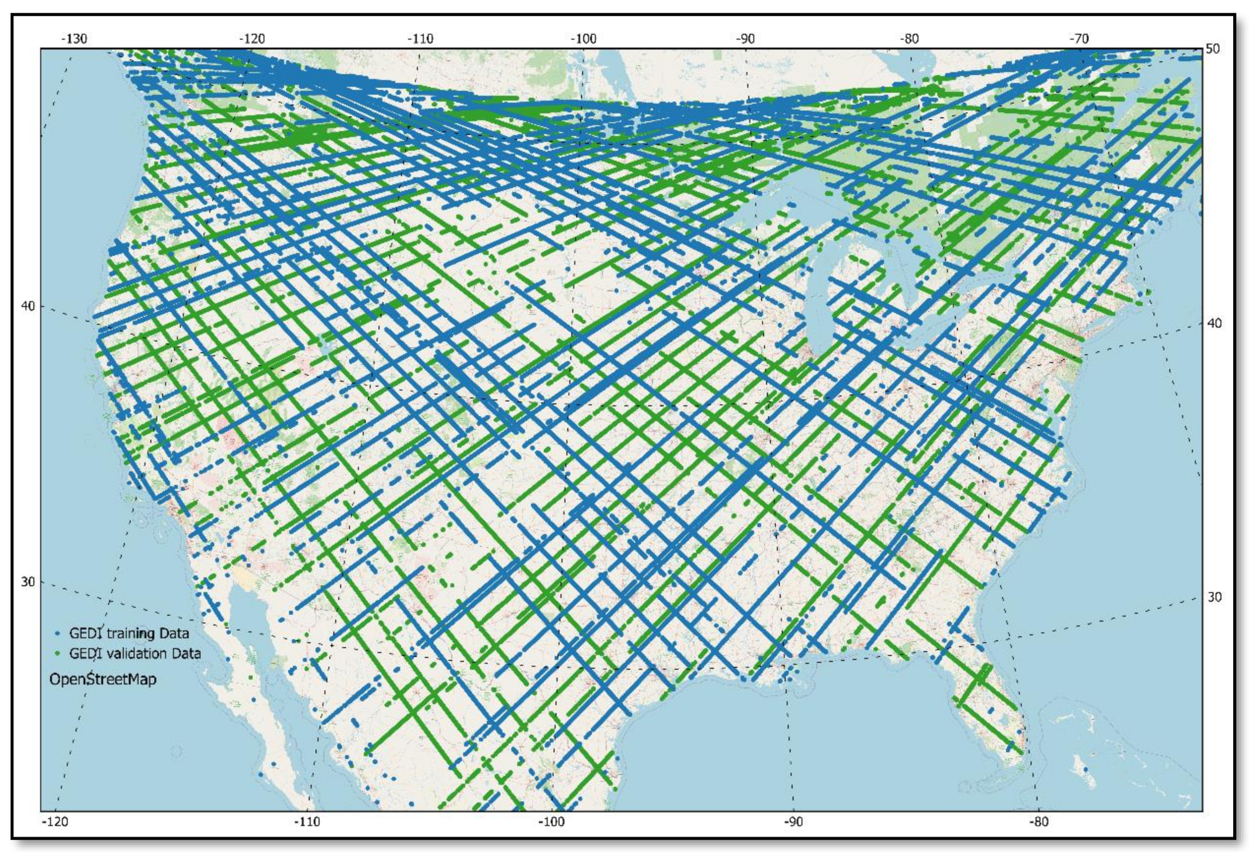
2.3. GEDI Data Processing

The GEDI level 02B product data granules [49] over North America were obtained for the two months of June and July 2019. Data from June and July were selected since for most of the conterminous US, except for some arid areas, tree canopy during the selected period is at or near full leaf out [23]. The obtained data contained 254,550,672 GEDI level 02B footprints of tree height, canopy cover, and vertical distribution of plant material. To select the highest quality data, the GEDI data were further filtered to remove the waveforms flagged as unsuitable for measuring canopy structure (“Quality flag” = 1), flagged as detector-saturated (“Degrade flag” = 1), or had sensitivity values <0.95. The sensitivity value of 0.95 was selected to reduce the proportion of false positive ground returns [50]. The application of these filters removed most of the data collected from the GEDI “coverage” beams, cloud-contaminated observations, and observations taken over water bodies [9,10]. The filtering resulted in a subset of 27,361,244 GEDI footprints or ~10.75% of the data collected over the study area during the two months of June and July.
The remaining GEDI level 02B data were then mapped into the VIIRS standard global 1-km Sinusoidal grid system. This resulted in 1,324,640 of collocated VIIRS-GEDI paired data records. The number of GEDI footprints falling within a collocated VIIRS grid cell ranged between 1 and 29 observations except for the VIIRS grid cells where the ascending and descending GEDI tracks intersected. In the latter case, the maximum number of GEDI observations falling within a VIIRS grid cell reached a maximum of 59 observations. Some 349,634 (or 26.4%) of the collocated VIIRS-GEDI grid cells contained 20 or more GEDI footprints and 580,744 (or 43.8%) of the collocated VIIRS-GEDI grid cells contained 10 or less GEDI footprints. The remaining VIIRS grid cells (394,471) contained 11 to 19 GEDI footprints.
The average values of GEDI products within the coincident VIIRS grid cells were calculated in order to investigate the relation between VIIRS and GEDI data products. The output are metrics of GEDI-VIIRS paired collections. However, only GEDI-VIIRS paired collections calculated from 20 or more GEDI observations were retained. The selection of the cutoff value of 20 was made to minimize the errors associated with under-sampling of GEDI observations within a VIIRS grid cell while maintaining a sufficiently large sample of GEDI-VIIRS paired collections that can capture variations in canopy structure across the study area. The resulting GEDI-VIIRS metrics contained 349,634 paired records relating VIIRS data to GEDI-derived CH, CFC, PAI, and FHD.
The GEDI-VIIRS paired collections were split into calibration and validation subsets. The calibration subset was drawn from a random sampling of half of the downloaded GEDI tracks. The validation subset were derived from the remaining GEDI tracks (Figure 1). Selecting independent GEDI tracks for model calibration and validation, especially when the geographic position is included as an explanatory variable, should reduce the impacts of spatial autocorrelation on model validation results [43,51]. The resulting GEDI-VIIRS training subset contained 162,477 paired records, whereas the validation metrics contained 187,157 paired VIIRS-GEDI records.

2.4. Calibration and Validation of the Random Forest Regression Models

The paired GEDI-VIIRS calibration data were used to train four random forest regression models [52] that can predict GEDI-like CH, CFC, PAI, and FHD. In total, 159 VIIRS-derived multi-temporal phenology metrics (Table 2) were used as input features (i.e., independent variables) in model construction.
Random forest regression models are an ensemble learning method. The method grows a user-defined number of regression trees and averages their predictions. In random forests, each tree in the ensemble (i.e., forest) is built from a sample drawn with replacement (i.e., a bootstrap sample) from the training set. Furthermore, when splitting each node during the construction of a tree, the best split is found either from all input features or from a random subset of inputs defined by the user [52]. The size of the subset of inputs and other regression tree model hyper-parameters (e.g., number of trees in the forest, the maximum depth of the regression trees, the minimum number of training samples required to split a node, and the minimum number of training sample to form a leaf) that produce optimal model performance can be estimated by an exhaustive search over user specified parameter values or through a randomized sampling from a user specified distribution of parameters settings [53].
To optimize model performance, the hyper-parameter values of the random forest models were approximated through a randomized sampling of 300 parameter setting. The 300 hyper-parameter samples were obtained from the distributions outlined in Table 3. Accordingly, a total of 1200 random forest models were evaluated (300 for each of the four random forest regression models). A randomly selected subset of the calibration data (15% of the calibration dataset) were used to search for the optimal hyper-parameter values. The use of only 15% of calibration data to tune the hyper-parameters of the models was done to maintain a reasonable utilization of computing resources.
The hyper-tuned random forest model parameters that better explained the out of bag sample variances of the GEDI-derived CH, CFC, PAI, and FHD (i.e., the models with the highest evaluated r2 value) were retained (Table 4). The retained hyper-parameters were subsequently used to calibrate four random forest regression models using the complete training dataset of 162,477 paired GEDI-VIIRS records. Model hyper-parameter and model calibration were performed using the Scikit-learn platform in Python [53].
Model validation was performed on the independent validation sample of 187,157 GEDI-VIIRS paired records derived from the GEDI granules not used in model calibration (see Section 2.3 for more details). The spatial distribution of the validation sample is shown in Figure 1. The four calibrated random forest regression models were then used to predict the four canopy structural elements CH, CFC, PAI, and FHD using VIIRS phenology metrics as model inputs. These VIIRS-derived CH, CFC, PAI, and FHD were compared to their corresponding GEDI-derived values in order to evaluate the performances of the four random forest regression models. The evaluation criteria were the ability of the models to explain the variances observed in the GEDI-derived canopy structural elements (R squared values as a measure of the precision of the models); and the accuracy of the four models measured by calculating the mean and median absolute errors as well as the root mean-squared error (RMSE). We also investigated model bias by calculating the distribution of differences between model-derived canopy structural elements and their corresponding GEDI-derived values at multiple intervals of the variables’ distribution.

2.5. Derivation and Assessment of Vegetation Structure Attributes for CONUS

The calibrated random forest regression models were applied to the 2019 multi-temporal phenology metrics (Table 2) in order to produce wall-to-wall maps of canopy height, fraction canopy cover, plant area index, and foliage height diversity index for the conterminous US. In producing the wall-to-wall maps, water bodies were not processed since the GEDI data used in model calibration did not include observations over water. The 926.65-m grid size water mask was calculated from the global 231.66-m land/water product [54]. Any 926.65-m was flagged as a water pixel if any of the 16 spatially coincident pixels in the original product were classified as water pixels.
Summary statistics and histograms were used to assess variations in the spatial distribution of the VIIRS-derived forest attribute values between ecoregions. The ecoregion boundaries used were the Environmental Protection Agency (EPA) level 1 and level 3 ecoregion boundaries. EPA ecoregions are identified by analyzing the patterns and composition of biotic and abiotic phenomena that affect or reflect differences in ecosystem quality and integrity [55,56,57]. Spatial patterns of forest structure attributes were expected to conform to the boundaries of EPA ecoregions since the biotic and abiotic phenomena used to delineate the ecoregions include geology, landforms, soils, vegetation, climate, and land use; all factors known to influence potential natural vegetation, its type and structure.

3. Results

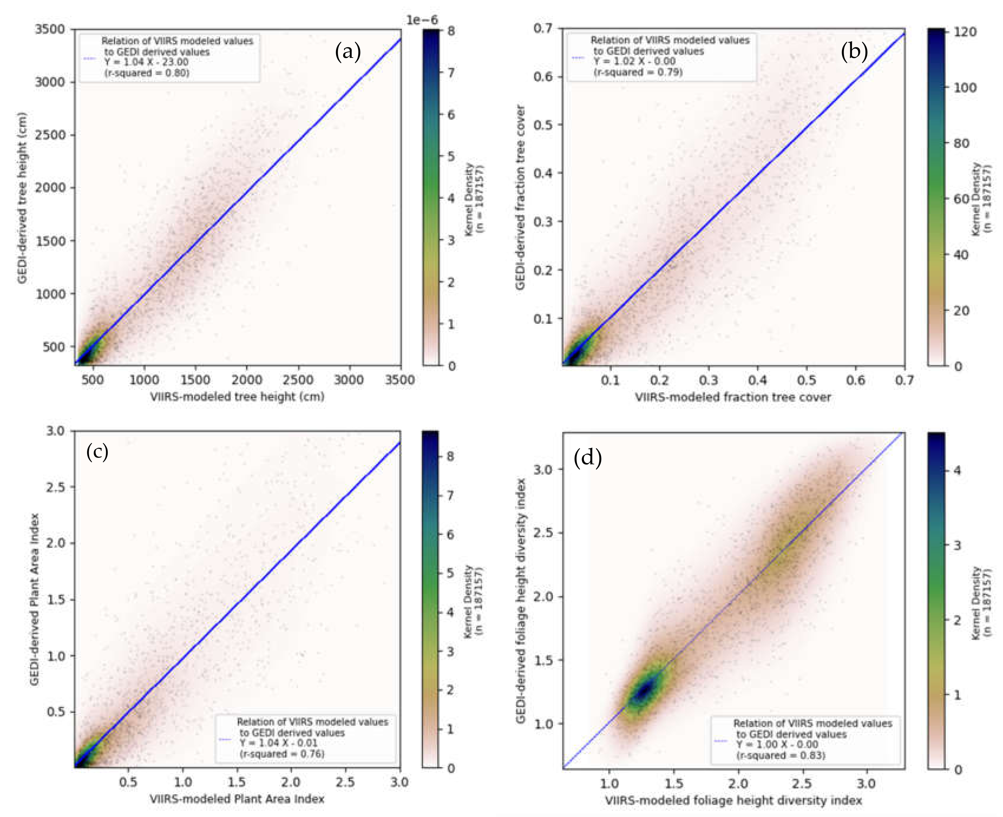
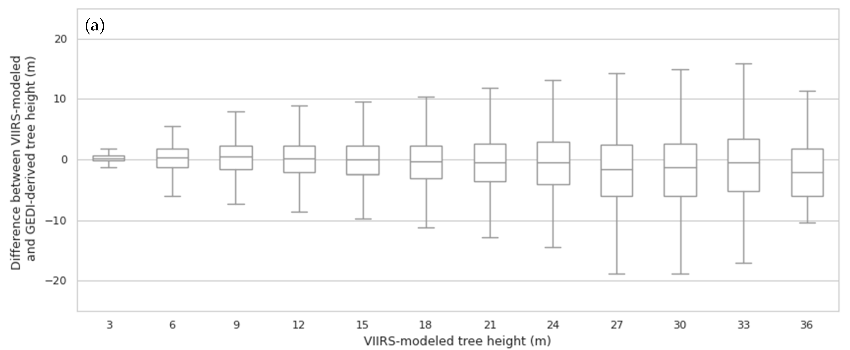
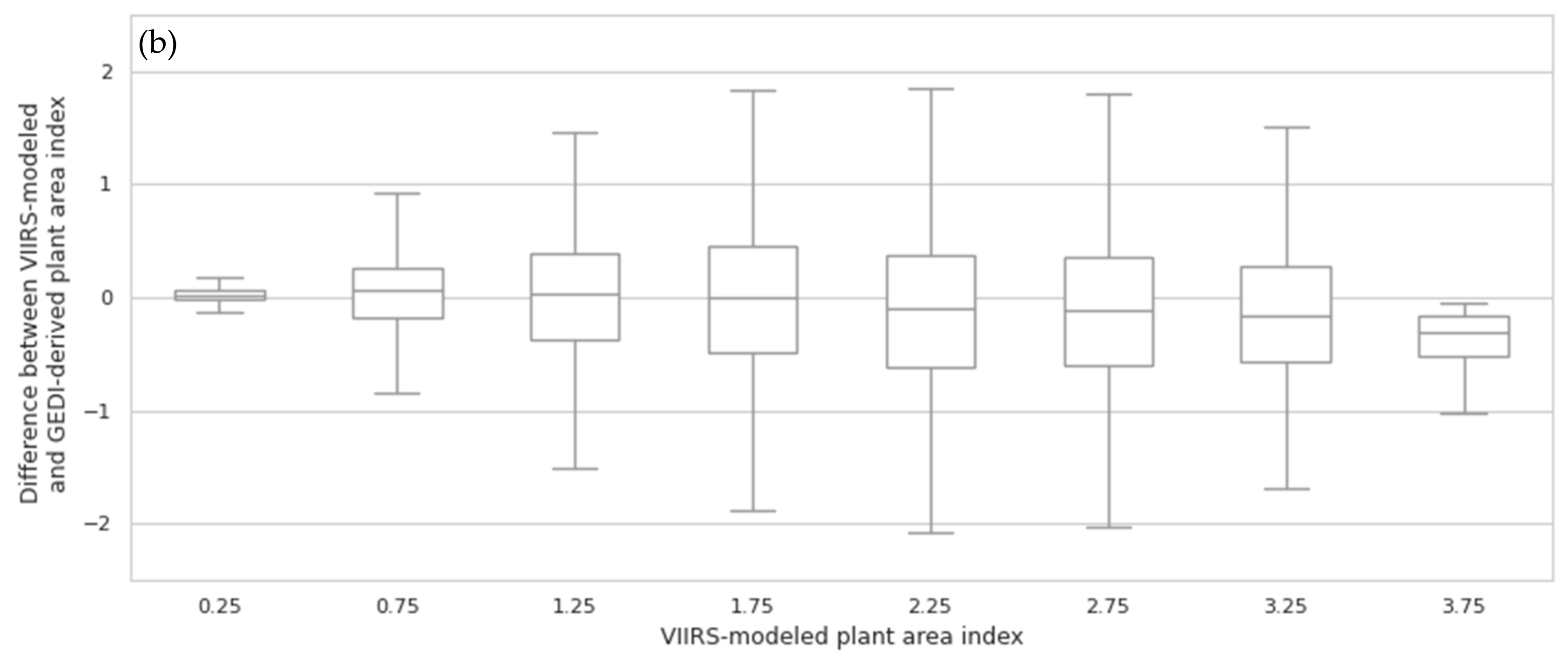
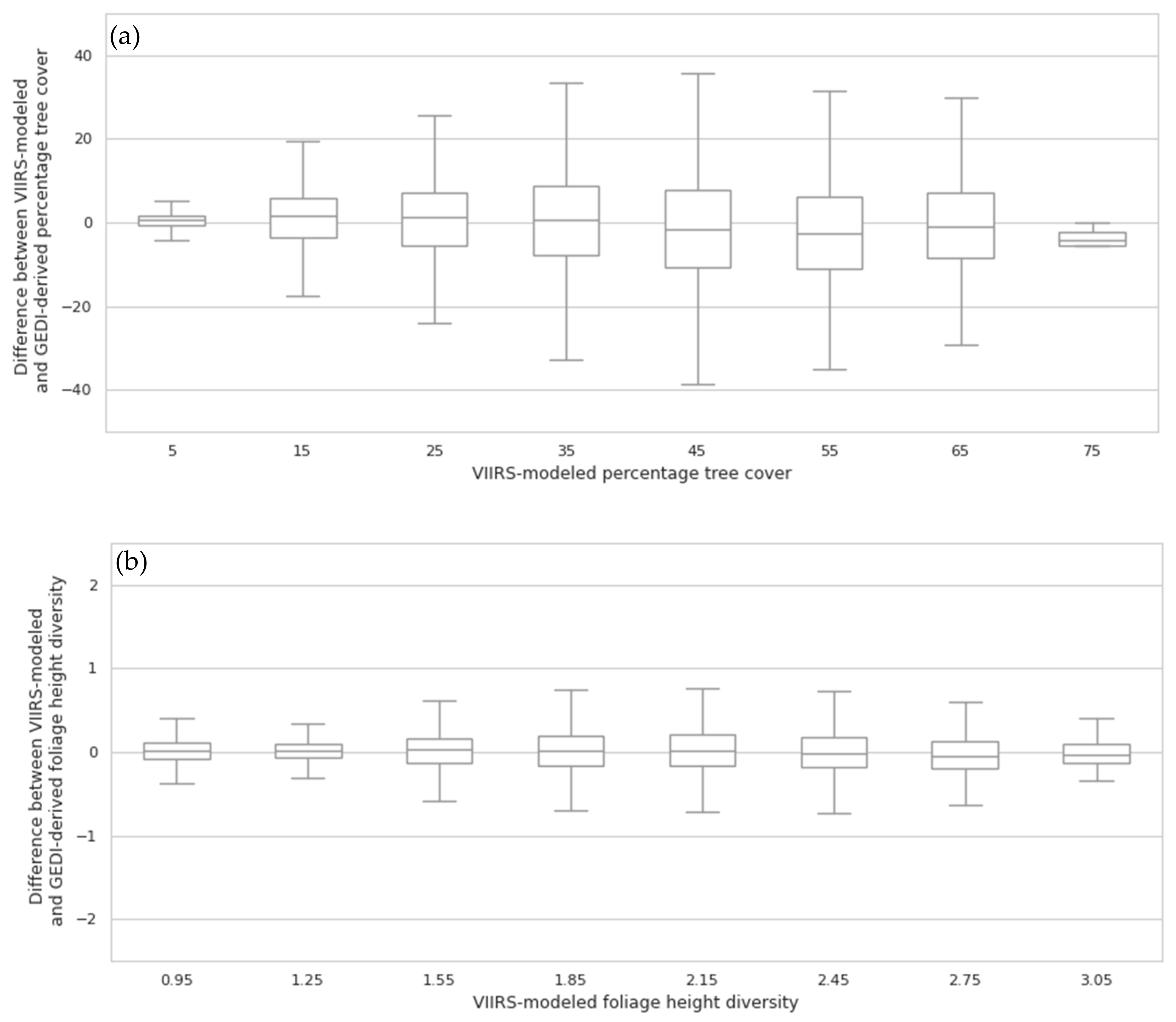
3.1. Random Forest Model Validation

Results from the comparison of the VIIRS-derived canopy attributes with their corresponding GEDI-derived attributes are summarized in Table 5. The precision (degree to which variations in GEDI-derived values were explained by the models) of the FHD model was higher (r2 = 0.83) than that for the other models with the PAI model having the lowest precision (r2 = 0.76).
When calculated over the entire data range, comparisons between the modeled and GEDI-derived values had negligible bias and offset values (Figure 2). However, when the distribution of the differences between the VIIRS-derived and the GEDI-derived values were plotted for strata representing intervals drawn from the range of each canopy attribute, it was noticed that the canopy height model underestimated GEDI-derived canopy height data for tall (>27 m) forests and the Plant Area Index model underestimated the GEDI-derived Plant Area Index at index values greater than 2 (Figure 3). Underestimation of fraction tree cover in denser forests were less pronounced while the comparisons of FHD values showed good correspondence between the modeled and reference data for all strata (Figure 4).

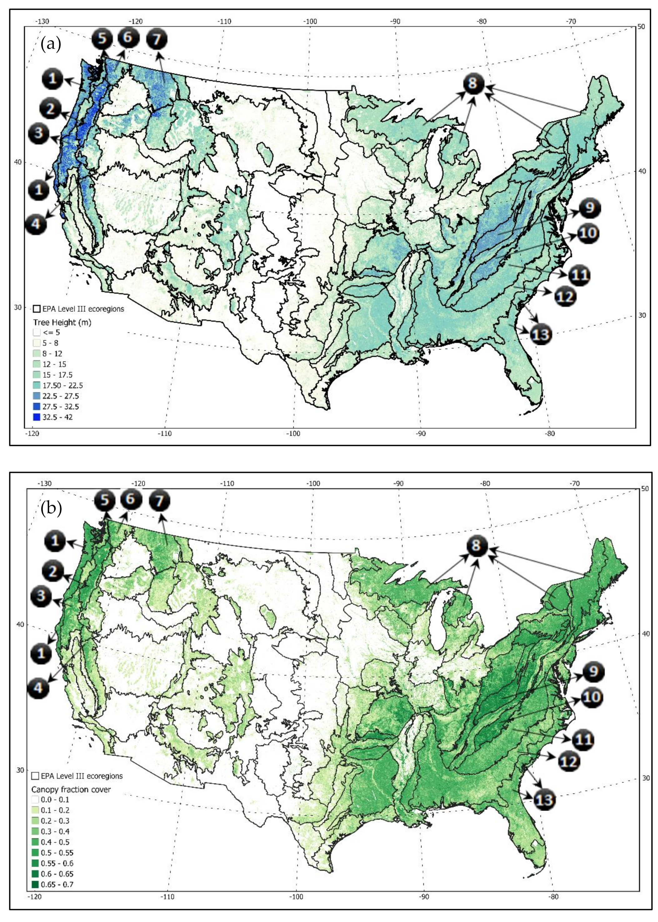
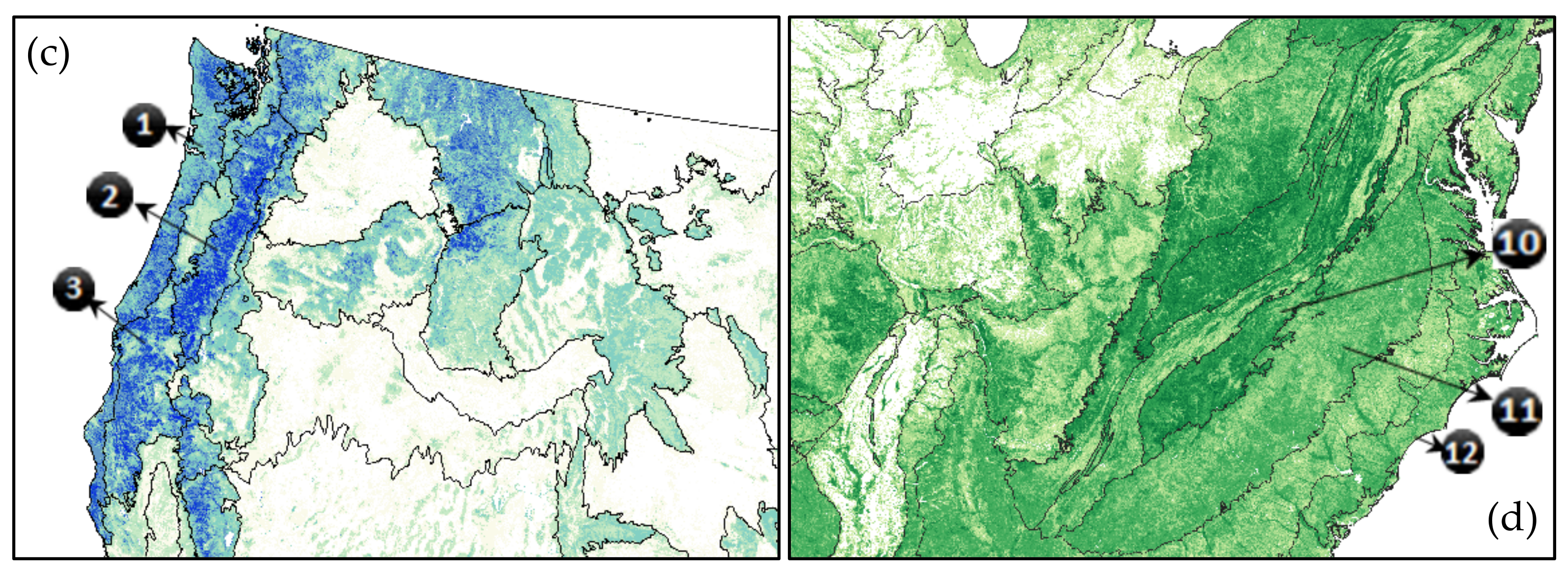
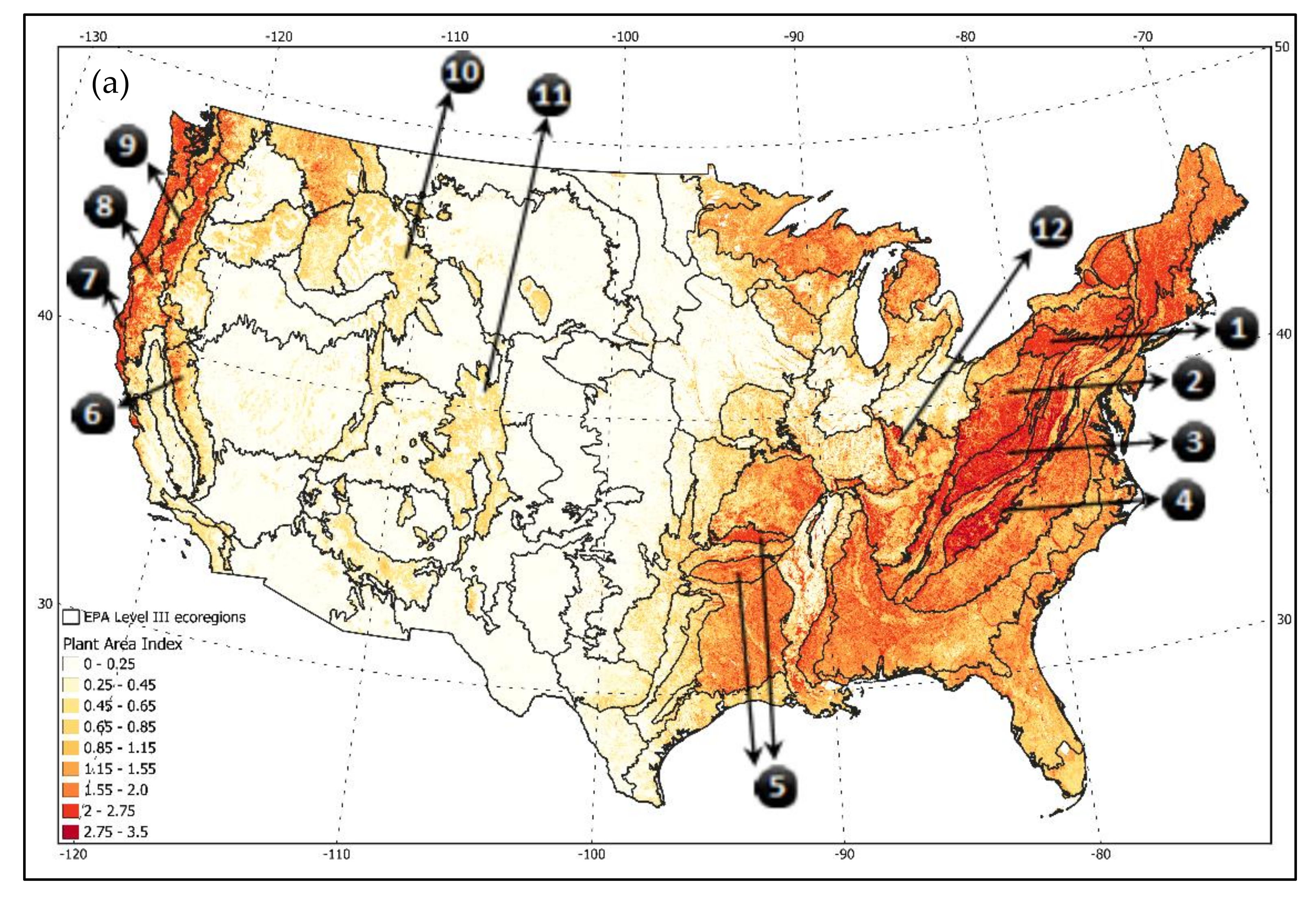
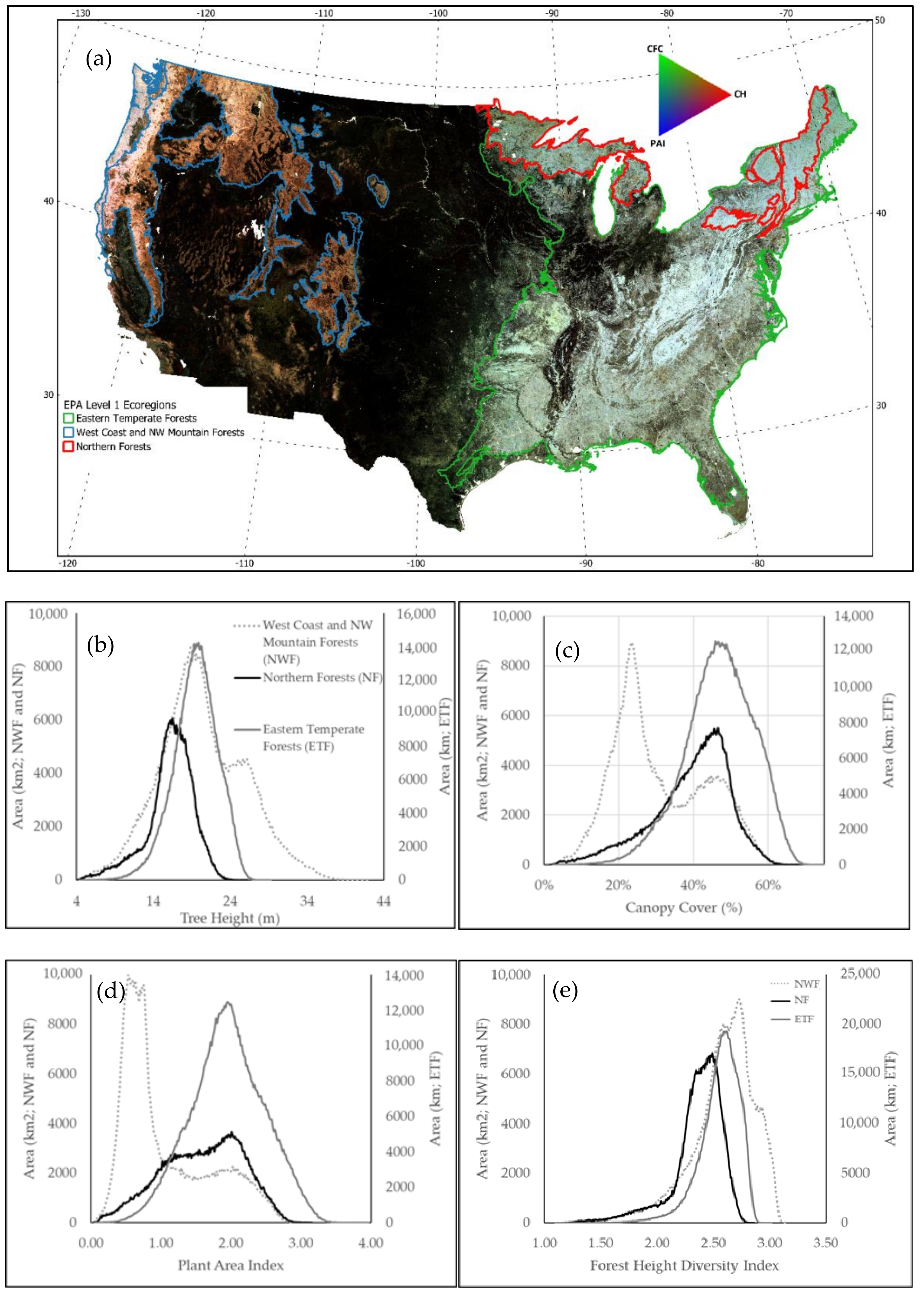
3.2. Wall-to-Wall Maps of Canopy Structure for the Conterminous US

The four random forest regression models were used to extrapolate from GEDI products wall-to-wall maps of canopy height, canopy fraction cover, plant area index, and foliage height diversity for the conterminous US using the phenology metrics derived from the observations acquired by the VIIRS instrument onboard the NOAA-20 satellite for the year 2019. Overlaying the EPA ecoregions on these maps showed distinct variations in the spatial patterns of forest structure attributes between EPA level III ecoregions (Figure 5 and Figure 6). This was expected since the factors that were used to delineate the ecoregion boundaries reflect the aggregate of geographic characteristics (both natural and anthropogenic) that determine potential vegetation, its type, horizontal distribution, and vertical profiles. The remainder of this section further examines the relation of EPA ecoregions to the VIIRS-derived forest attributes.
The VIIRS-modeled canopy height map (Figure 5a) demonstrated canopy height (CH) variations across natural forest and ecoregion types in the conterminous US. The tallest modeled tree heights were in the Klamath Mountains and the Cascades of the Northwestern Forested Mountains as well as in the coast range of the Marine West Coast Forests (Figure 5c). These ecoregions are habitats for very tall conifer species including the coast Douglas-fir (Pseudotsuga menziesii ssp. menziesii), the Western Red Cedar (Thuja plicata), the coast Redwood (Sequoia sempervirens), and Sitka Spruce (Picea sitchensis). The next modeled tallest trees were in the North Cascades, Eastern Cascade slopes and foothills, and in the northern reaches of the Sierra Nevada range. These regions are also home to the tall coniferous species of Douglas-fir, Western Red Cedar, and Jeffrey pine (Pinus jeffreyi). Similarly, modeled tree height results suggest that some forested regions in the Northern Rockies are also taller than the Eastern temperate forests and the Northern Hardwood Forests of the US (Figure 5a and Figure 7a). Modeled canopy height values in the Eastern Temperate forests also show height variation related to natural forest types, clearly separating taller Appalachian and Blue Ridge Mountain forests from lower canopy height forests of the Piedmont Plateau, the Southeastern Plains, and the Southern Coastal Plains (Figure 5a). However, the forests of the Piedmont Plateau were, in general, taller than the northern hardwood forests of the Great Lakes (Figure 7b).
Results from the canopy fraction cover (CFC) model showed several ecoregions with expansive forests characterized by high percentage canopy cover (Figure 5b). For example, the landscapes of the Blue Ridge and the Central Appalachians (Figure 5d) had a median VIIRS-derived percentage canopy cover greater than 55%. In general, most of the natural forest types of the Eastern Temperate forests had a median VIIRS-derived canopy fraction cover exceeding that of the forests of the Northwestern Forested Mountains except for the sub ecoregions of the cascades and the Coast Range (Figure 7c). The latter sub-regions had median percentage cover values comparable to the Eastern Temperate Forests and the Northern hardwood forests.
VIIRS-modeled Plant Area Index (PAI) values were found to be higher in forests with tall trees and high percentage canopy cover (Figure 6a). Large areas of the Blue Ridge and the Central Appalachians had PAI values greater than 2.75. In comparison, fewer forested areas had PAI values greater than 2.75 in the South-Western Appalachians, the Western Allegheny Plateau, and in the Northwestern parts of the Interior Plateau (Figure 6c). Some patches of the tall forests in the Cascades, Coast Range, and to a lesser extent in the Klamath mountains ecoregions had VIIRS modeled PAI values between 2.0 and 2.75. Large areas with relatively high VIIRS-modeled PAI values were also found in Ouachita/Boston Mountains ecoregions, and Northern Appalachian/Maritime Highlands. Except for the Cascades and Coast range, most of the Northwestern Forested Mountains had lower PAI than the Northern Hardwood Forests and the Eastern Temperate Forests (Figure 7d).
The spatial arrangements of the VIIRS-modeled foliage height diversity (FHD) values showed different spatial patterns from those for PAI, CFC, and CH (Figure 6b). Compared to other ecoregions with similar canopy height, and canopy fraction cover, the FHD values over large areas of the Sierra Nevada range were surprisingly high (Figure 6d). Similarly, the relatively shorter and sparse coniferous forests of the Middle and Southern Rockies ecoregions had, on average, similar FHD values to the taller and denser canopies of Klamath Mountains. In general, median FHD values were highest in the Northwestern Forested Mountains followed by the Eastern temperate forest, and the lowest median FHD values were modeled for the Northern Hardwood Forests (Figure 7e). The distribution of very high FHD values were in the sub-regions of the Appalachians, Ouachita/Boston Mountains ecoregion, the Cascades, Klamath Mountains, and large swaths of the Sierra Nevada range (Figure 6b).
The multiband color rendering of CH (red band), CFC (green band), and PAI (blue band) further illustrates how these three forest structural attributes vary across the CONUS (Figure 7a). The color intensity of the Red-Green-Blue bands in Figure 7a is linearly related to the spatial distribution of its corresponding forest structure attribute values. Compared to other forests in the CONUS, forests with relatively high CH, CFC, and PAI values are rendered in white tones such as in the 
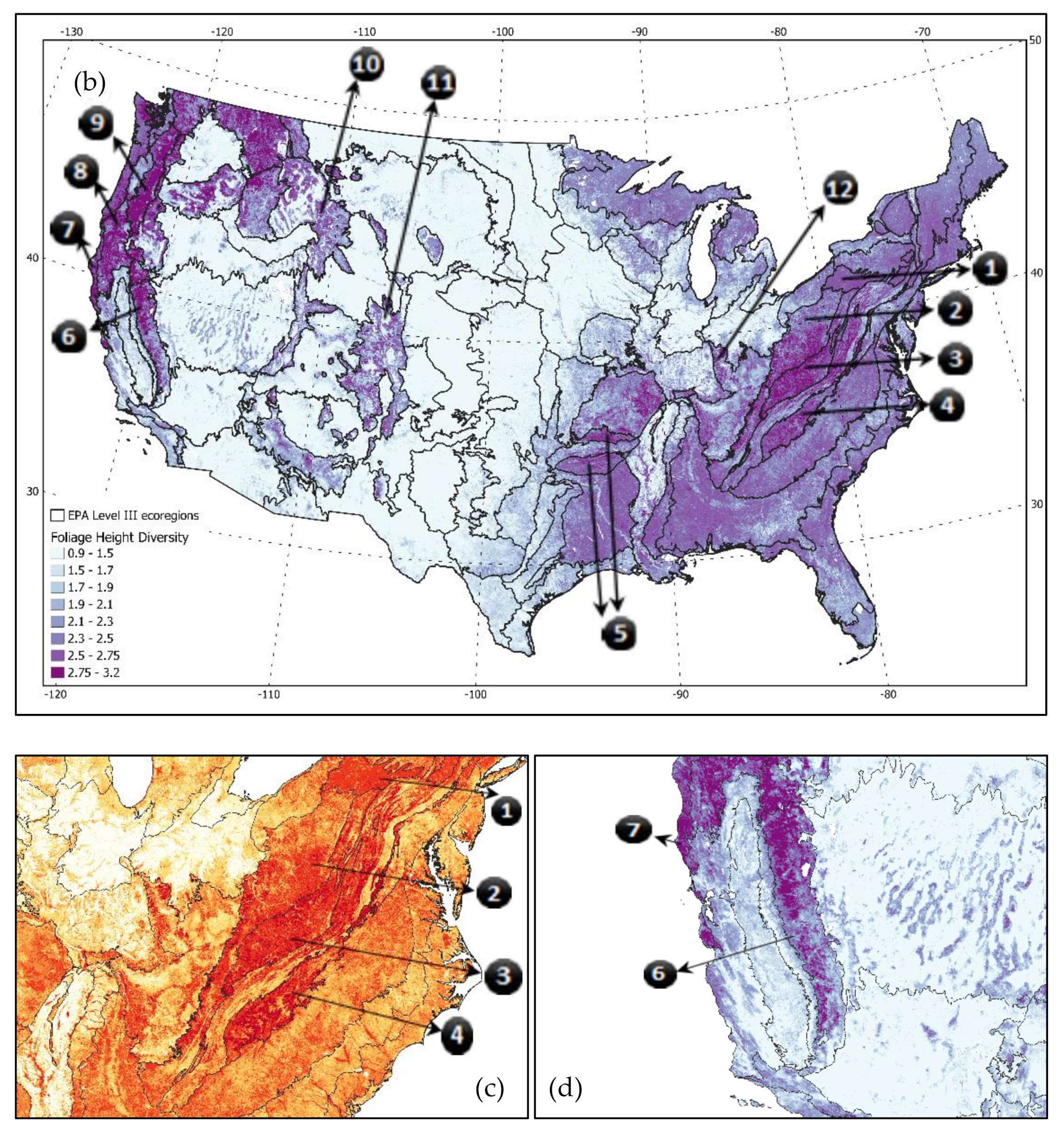
Marine West Coast Forests, the Cascades, and Central Appalachians. Darker red/orange tones such as in the central and northern Rockies represent more open canopy with relatively tall trees. Darker green tones such as in the Piedmont Plateau represent dense canopy with relatively shorter trees. Black tones in Figure 7a are non-forested areas.

4. Discussion

After its nominal two-year lifetime, GEDI will have covered the majority of 1-km cells between 51.6° N and S with two or more ground tracks [34]. However, cloud contamination, track spacing, clumping in the ISS orbital tracks, and removal of GEDI waveforms unsuitable for measuring canopy structure can result in large coverage gaps at the 1-km grid [31,58]. In this study, only 10.75% of the GEDI footprints were retained after filtering out waveforms flagged as “low quality” and waveforms with a sensitivity value <0.95. The estimation of forest structure attributes for the 1-km grid cells that have few or zero “high quality” GEDI waveforms can benefit from using statistical models that integrate GEDI-derived forest structure data with wall-to-wall satellite images [31,58]. Similarly, the GEDI L4B 1-km gridded science data product will use statistical models that utilize wall-to-wall satellite images to estimate above ground biomass in grid cells with less than two coincident GEDI ground tracks [10].
This study demonstrated the potential of using random forest regression models and VIIRS data to extrapolate the GEDI-derived forest structure attributes into wall-to-wall maps of CH, CFC, PAI, and FHD. It should be noted that the GEDI and VIIRS-derived PAI are different from True PAI and LAI since large-footprint LiDAR systems cannot directly measure leaf clumping or leaf angle distribution. End users are therefore recommended to apply conversions based on their best knowledge to convert GEDI’s PAI to true PAI and LAI for running earth system models [30].
The accuracy of the modeled results in this study depended on several factors, notably the quality and availability of reference LiDAR data, the quality and consistency of the optical VIIRS data, and any limitations of the ability of the statistical models, to accurately predict the outputs without bias. One factor which could have affected the generalization ability of the models was the number of cloud-free “high-quality” GEDI observations used to calculate the mean values of the canopy structural attributes within the 1-km VIIRS grid cell. The number of GEDI observations ranged between 20 and 59. Especially in heterogeneous landscapes, under-sampling can result in high mean standard errors [59] and thus in inaccurate representation of canopy structural attributes at the 1-km resolution grid cell [34,43]. The availability of GEDI observations is expected to increase as soon as the data collected during the full leaf-out period in 2020 become publically available. Furthermore, the expected future availability of more GEDI data will increase the size of the GEDI-VIIRS training sample for some of the currently underrepresented surface types (e.g., human settlements and landscapes with frequent cloud cover). Therefore, the expected increase in GEDI data availability should increase the accuracy of model outputs.
In addition to GEDI data availability, other issues still exist in GEDI data that can affect model performance. Surface slopes, for instance, can affect tree height estimation by LiDAR instruments [60,61]. While the GEDI footprint size was selected to limit the vertical mixing of vegetation and ground signals caused by surface slope [10], comparisons of the GEDI height metric (RH95) with airborne laser scanning (ALS) data in [9] revealed that RH95 tends to overestimate canopy height in areas of complex topography and sparse tree cover. Additional corrections of the footprint-level data may therefore be required to reduce slope-induced canopy height uncertainty [9]. Furthermore, residual geolocation errors of GEDI data were also found to affect the calibration and validation of the statistical models [9]. Currently available GEDI data from [62] has a horizontal geolocation accuracy between 10 and 20 meters [10] which was found to affect the performance of Landsat-based tree height models [9]. Future calibration process is expected to reduce the geolocation error down to 8 m horizontal [10]. Nonetheless, the impacts of surface slopes and residual geolocation errors on the results of this study should be less pronounced than the impacts surmised in studies utilizing higher spatial resolution optical data [9]. Aggregating LiDAR data to a 1-km grid cell size is expected to reduce model uncertainty due to spatial averaging of errors [5,59,63,64,65,66]. For instance, the impacts of LiDAR positioning errors on biomass prediction errors [63,64] and on the prediction errors of tree canopy attributes [66] were all found to decrease exponentially with mapping resolution [59]. A theoretical analysis on how spatial aggregation can reduce spatial random noise and improve the accuracy and precision of predictive models is presented in [67].
In addition to inherent errors in GEDI data, validation results using the reserved sample of 187,157 VIIRS-GEDI observations showed an underestimation of canopy height for tall (>27m) forests and an underestimation of Plant Area Index at index values greater than 2.5. Other studies integrating LiDAR and optical data using regression forests (RF) or regression trees similarly reported an underestimation of tree height in tall forests [9,68]. This might be due to (1) the problematic behavior of the random forest regression models in situations where the training and prediction inputs differ in their range and/or distributions (i.e., covariate shift); (2) the low sampling rate in the training data of very tall forests; (3) the loss of sensitivity of optical data, especially in the visible spectrum, to increasing LAI/PAI values [26,27,69]; and (4) due to the previously discussed errors in the GEDI training data. Highly localized calibration of Landsat-based models of canopy height were found in [70] to improve model performance and reduce model biases at either edge of the data range. Substituting RF models with Deep Learning models might reduce model biases at the higher end of the distribution of canopy height and PAI values. Indeed, recent applications of deep learning (DL) regression models to retrieve continuous canopy structural attributes [68,71,72] showed promising results. DL models were found in [68] to outperform RF models in mapping canopy height in Northwestern China. Convolutional Neural Networks (CNNs) applied to Sentinel-2 data to estimate vegetation height were demonstrated to have better sensitivity to the taller canopy heights in [72] than RF models applied to Landsat data in [9] and to VIIRS-data in this study.
It should be stressed that while the resulting 1-km VIIRS-derived maps of forest attributes showed good agreements with the GEDI-validation data, the GEDI-VIIRS comparisons cannot be construed as accuracy assessments of the derived 1-km maps. These comparisons are a representation of the ability of the models to extrapolate GEDI-like forest structure attributes across the CONUS. A robust accuracy assessment should consider the errors in the GEDI-derived products. Results from the GEDI pre-launch calibration and validation studies suggested GEDI ability to measure subtle variations in the complex vertical canopy structure [50] at sub-meter vertical accuracy [10,30]. Several studies also demonstrated the added value of incorporating simulated GEDI data into models that map forest structure and biomass from space-born Interferometric Synthetic Aperture Radar data [31,58,73]. However, the accuracies of post launch GEDI data and products might differ from the accuracies of the ALS-simulated GEDI data due to, for example, geolocation inaccuracies, and spatiotemporal variations in atmospheric attenuation. A robust post-launch validation is needed to assess the accuracy of GEDI science data products. A robust post-launch validation requires contemporaneous reference data (e.g., Terrestrial Laser Scanning and Airborne Laser Scanning data) that are collocated with on-orbit GEDI data, and encompasses a broad range of tropical and temperate vegetation types. The acquisition and processing of these data is a global collaborative effort that is being coordinated by the GEDI calibration and validation program. These reference data, once available, will be used by the GEDI team to validate GEDI performance against design requirements, assess the repeatability of the GEDI level 1 and 2 product variables, and verify their accuracy [10].
Other approaches are currently being tested to produce 1-km or finer scale wall-to-wall maps of 3D vegetation structure. These include a spatially interpolated GEDI-derived level 3 gridded canopy vegetation metrics [10], the fusion of GEDI with interferometric SAR [31,58,74,75], and the fusion of GEDI and ICESAT-2 data with moderate (10–30 m) resolution optical remote sensing data [9,68,72]. While Sentinel-1/2 and Landsat data were utilized to derive tree height and tree cover products at much finer spatial detail [9,68,72] than the VIIRS-derived products, they can be subject to data gaps in cloudy regions and in regions with sparse Landsat/Sentinel-2 data record. Compared to finer spatial resolution sensors, the VIIRS very high data acquisition rate reduces the effects of clouds and incomplete atmospheric correction on the temporal consistency of VIIRS data which should in turn reduce spatial and inter-annual fluctuations in modeled results that would otherwise be caused by atmospheric contamination. Furthermore, the generalization ability of parametric and non-parametric statistical models was found to be inversely related to spatial scale [59,64] as a results of the spatial aggregation of errors [5,63,64,65] and because aggregation reduces the contamination of a pixel reflectance values from reflected light originating beyond the pixel’s area (i.e., aggregation reduces the impacts of the sensor’s point spread function or PSF) [76].
Improving the accuracy of the statistical models will enable a more precise analysis of inter-annual and multi-decadal forest dynamics. Robust models will enable the annual monitoring of changes in forest structural attributes. This is essential for monitoring post disturbance forest regrowth, forest degradation, and carbon emissions from land conversions. It is expected that more robust models can be achieved by (1) the increased availability of the GEDI data; (2) the planned improvements to the GEDI data and the quality of its products [9,10]; (3) and tuning the hyper-parameters and parameters of deep learning algorithms.

5. Conclusions

Accurate, multi-year, 3D vegetation structure data at spatial resolutions of 1-km or less are needed by the ecosystem science community to constrain the errors associated with modeling above ground biomass (AGBM), Net Ecosystem Exchange (NEE), and Carbon fluxes associated with forest disturbance events and post-disturbance forest recovery [1]. The higher the accuracy of the derived 3D vegetation structure, the more feasible it is to precisely model biomass and Carbon fluxes especially where the scale of mapping matches the important scales of vegetation dynamics and the underlying environmental gradients [1].
This study demonstrated the feasibility of integrating GEDI-derived tree canopy structure data with VIIRS-derived multi-temporal phenology metrics to produce contiguous maps of tree canopy height, canopy fraction cover, plant area index, and foliage height diversity. Unfortunately, the limited availability of reference data did not allow for a robust accuracy assessment that considers the propagation of the errors that resulted from using the modeled GEDI forest structure products. Nevertheless, if the GEDI-derived tree canopy data do provide a valid representation of canopy 3D structure as suggested by GEDI pre-launch validation studies, the VIIRS-derived maps produced in this study can assist in modeling the true magnitude of global forest biomass stocks and for prognosticating future trends in the strength of the land carbon sink.
Future endeavors will focus on increasing the robustness of the statistical models to enable multi-decadal monitoring of forest dynamics at global scale using the entire VIIRS-NPP and MODIS data records. Extending the methods presented in this study to global coverage may require training separate models for each biome or for each vegetation type as suggested in [9,72] in order to overcome the limitations of model overfitting when employing very large training datasets.
Furthermore, it will be worthwhile to evaluate the potential of developing global 3D vegetation structure data using the VIIRS 350m I bands with a precision that is sufficient to calculate about 80% accurate 500 m biomass maps as this would represent a significant advance forward and provide the most accurate baseline map of carbon stocks to date [10].

Author Contributions

Conceptualization, C.H., K.R., and X.Z.; methodology, C.H. and K.R.; computer code, K.R.; validation, K.R.; writing—original draft preparation, K.R.; writing—review and editing, K.R., C.H., and X.Z. All authors have read and agreed to the published version of the manuscript.

Funding

This study was supported by NOAA grant NA19NES4320002 (Cooperative Institute for Satellite Earth System Studies -CISESS) and NOAA grant NA14NES4320003 at the University of Maryland/ESSIC. Additional support for Khaldoun and Huang was provided by NASA through grant 80NSSC18K0833 and US Fish and Wildlife Service through grant F18AC00973.

Data Availability Statement

Publicly available datasets were analyzed in this study. GEDI data were obtained from https://search.earthdata.nasa.gov/ and VIIRS data were obtained from NOAA’s Comprehensive Large Array-data Stewardship System (https://www.avl.class.noaa.gov/).

Conflicts of Interest

The authors declare no conflict of interest. The funders had no role in the design of the study; in the collection, analyses, or interpretation of data; in the writing of the manuscript, or in the decision to publish the results. The manuscript contents are solely the opinions of the authors and do not constitute a statement of policy, decision, or position on behalf of NOAA or the U.S. Government.

References

  1. Hall, F.G.; Bergen, K.; Blair, J.B.; Dubayah, R.; Houghton, R.; Hurtt, G.; Kellndorfer, J.; Lefsky, M.; Ranson, J.; Saatchi, S.; et al. Characterizing 3D Vegetation Structure from Space: Mission Requirements. Remote Sens. Environ. 2011, 115, 2753–2775. [Google Scholar] [CrossRef] [Green Version]
  2. Houghton, R.A. Aboveground Forest Biomass and the Global Carbon Balance. Glob. Chang. Biol. 2005, 11, 945–958. [Google Scholar] [CrossRef]
  3. Pereira, H.M.; Ferrier, S.; Walters, M.; Geller, G.N.; Jongman, R.H.G.; Scholes, R.J.; Bruford, M.W.; Brummitt, N.; Butchart, S.H.M.; Cardoso, A.C.; et al. Essential Biodiversity Variables. Science 2013, 339, 277–278. [Google Scholar] [CrossRef] [PubMed] [Green Version]
  4. Mitchard, E.T.; Saatchi, S.S.; Baccini, A.; Asner, G.P.; Goetz, S.J.; Harris, N.L.; Brown, S. Uncertainty in the Spatial Distribution of Tropical Forest Biomass: A Comparison of Pan-Tropical Maps. Carbon Balance Manag. 2013, 8, 10. [Google Scholar] [CrossRef] [PubMed] [Green Version]
  5. Goetz, S.; Dubayah, R. Advances in Remote Sensing Technology and Implications for Measuring and Monitoring Forest Carbon Stocks and Change. Carbon Manag. 2011, 2, 231–244. [Google Scholar] [CrossRef]
  6. Forsell, N.; Turkovska, O.; Gusti, M.; Obersteiner, M.; den Elzen, M.; Havlik, P. Assessing the INDCs’ Land Use, Land Use Change, and Forest Emission Projections. Carbon Balance Manag. 2016, 11, 26. [Google Scholar] [CrossRef] [Green Version]
  7. Griscom, B.W.; Adams, J.; Ellis, P.W.; Houghton, R.A.; Lomax, G.; Miteva, D.A.; Schlesinger, W.H.; Shoch, D.; Siikamäki, J.V.; Smith, P.; et al. Natural Climate Solutions. Proc. Natl. Acad. Sci. USA 2017, 114, 11645–11650. [Google Scholar] [CrossRef] [Green Version]
  8. Fargione, J.E.; Bassett, S.; Boucher, T.; Bridgham, S.D.; Conant, R.T.; Cook-Patton, S.C.; Ellis, P.W.; Falcucci, A.; Fourqurean, J.W.; Gopalakrishna, T.; et al. Natural Climate Solutions for the United States. Sci. Adv. 2018, 4, eaat1869. [Google Scholar] [CrossRef] [Green Version]
  9. Potapov, P.; Li, X.; Hernandez-Serna, A.; Tyukavina, A.; Hansen, M.C.; Kommareddy, A.; Pickens, A.; Turubanova, S.; Tang, H.; Silva, C.E.; et al. Mapping Global Forest Canopy Height Through Integration of GEDI and Landsat Data. Remote Sens. Environ. 2020, 112165. [Google Scholar] [CrossRef]
  10. Dubayah, R.; Blair, J.B.; Goetz, S.; Fatoyinbo, L.; Hansen, M.; Healey, S.; Hofton, M.; Hurtt, G.; Kellner, J.; Luthcke, S.; et al. The Global Ecosystem Dynamics Investigation: High-Resolution Laser Ranging of the Earth’s Forests and Topography. Sci. Remote Sens. 2020, 1. [Google Scholar] [CrossRef]
  11. Knapp, N.; Fischer, R.; Huth, A. Linking Lidar and Forest Modeling to Assess Biomass Estimation across Scales and Disturbance States. Remote Sens. Environ. 2018, 205, 199–209. [Google Scholar] [CrossRef]
  12. Knapp, N.; Fischer, R.; Cazcarra-Bes, V.; Huth, A. Structure Metrics to Generalize Biomass Estimation from Lidar across Forest Types from Different Continents. Remote Sens. Environ. 2020, 237, 111597. [Google Scholar] [CrossRef]
  13. Köhler, P.; Huth, A. The Effects of Tree Species Grouping in Tropical Rainforest Modelling: Simulations with the Individual-Based Model Formind. Ecol. Model. 1998, 109, 301–321. [Google Scholar] [CrossRef] [Green Version]
  14. Hurtt, G.C.; Dubayah, R.; Drake, J.; Moorcroft, P.R.; Pacala, S.W.; Blair, J.B.; Fearon, M.G. Beyond Potential Vegetation: Combining Lidar Data and a Height-Structured Model for Carbon Studies. Ecol. Appl. 2004, 14, 873–883. [Google Scholar] [CrossRef] [Green Version]
  15. Hurtt, G.C.; Thomas, R.Q.; Fisk, J.P.; Dubayah, R.O.; Sheldon, S.L. The Impact of Fine-Scale Disturbances on the Predictability of Vegetation Dynamics and Carbon Flux. PLoS ONE 2016, 11. [Google Scholar] [CrossRef] [PubMed]
  16. Hurtt, G.; Zhao, M.; Sahajpal, R.; Armstrong, A.; Birdsey, R.; Campbell, E.; Dolan, K.; Dubayah, R.; Fisk, J.P.; Flanagan, S.; et al. Beyond MRV: High-Resolution Forest Carbon Modeling for Climate Mitigation Planning over Maryland, USA. Environ. Res. Lett. 2019, 14, 045013. [Google Scholar] [CrossRef]
  17. Schneider, F.D.; Ferraz, A.; Hancock, S.; Duncanson, L.I.; Dubayah, R.O.; Pavlick, R.P.; Schimel, D.S. Towards Mapping the Diversity of Canopy Structure from Space with GEDI. Environ. Res. Lett. 2020, 15, 115006. [Google Scholar] [CrossRef]
  18. Friedl, M.A.; McIver, D.K.; Hodges, J.C.F.; Zhang, X.Y.; Muchoney, D.; Strahler, A.H.; Woodcock, C.E.; Gopal, S.; Schneider, A.; Cooper, A.; et al. Global Land Cover Mapping from MODIS: Algorithms and Early Results. Remote Sens. Environ. 2002, 83, 287–302. [Google Scholar] [CrossRef]
  19. Hansen, M.C.; Defries, R.S.; Townshend, J.R.G.; Sohlberg, R. Global Land Cover Classification at 1 km Spatial Resolution Using a Classification Tree Approach. Int. J. Remote Sens. 2000, 21, 1331–1364. [Google Scholar] [CrossRef]
  20. Hansen, M.C.; Stehman, S.V.; Potapov, P.V. Quantification of Global Gross Forest Cover Loss. Proc. Natl. Acad. Sci. USA 2010, 107, 8650–8655. [Google Scholar] [CrossRef] [Green Version]
  21. Hansen, M.C.; Potapov, P.V.; Moore, R.; Hancher, M.; Turubanova, S.A.; Tyukavina, A.; Thau, D.; Stehman, S.V.; Goetz, S.J.; Loveland, T.R.; et al. High-Resolution Global Maps of 21st-Century Forest Cover Change. Science 2013, 342, 850–853. [Google Scholar] [CrossRef] [Green Version]
  22. Huang, C.; Zhang, R.; Zhan, X.; Csiszar, I. Derivation of Global Surface Type Products from VIIRS. In Proceedings of the IGARSS 2019—2019 IEEE International Geoscience and Remote Sensing Symposium, Yokohama, Japan, 28 July–2 August 2019; pp. 5992–5995. [Google Scholar]
  23. Zhang, X.; Liu, L.; Liu, Y.; Jayavelu, S.; Wang, J.; Moon, M.; Henebry, G.M.; Friedl, M.A.; Schaaf, C.B. Generation and Evaluation of the VIIRS Land Surface Phenology Product. Remote Sens. Environ. 2018, 216, 212–229. [Google Scholar] [CrossRef]
  24. Hansen, M.C.; DeFries, R.S.; Townshend, J.R.G.; Sohlberg, R.; Dimiceli, C.; Carroll, M. Towards an Operational MODIS Continuous Field of Percent Tree Cover Algorithm: Examples Using AVHRR and MODIS Data. Remote Sens. Environ. 2002, 83, 303–319. [Google Scholar] [CrossRef]
  25. Sexton, J.O.; Song, X.-P.; Feng, M.; Noojipady, P.; Anand, A.; Huang, C.; Kim, D.-H.; Collins, K.M.; Channan, S.; DiMiceli, C.; et al. Global, 30-m Resolution Continuous Fields of Tree Cover: Landsat-Based Rescaling of MODIS Vegetation Continuous Fields with Lidar-Based Estimates of Error. Int. J. Digit. Earth 2013, 6, 427–448. [Google Scholar] [CrossRef] [Green Version]
  26. Price, J.C. Estimating Leaf Area Index from Satellite Data. IEEE Trans. Geosci. Remote Sens. 1993, 31, 727–734. [Google Scholar] [CrossRef]
  27. Knyazikhin, Y.; Martonchik, J.V.; Diner, D.J.; Myneni, R.B.; Verstraete, M.; Pinty, B.; Gobron, N. Estimation of Vegetation Canopy Leaf Area Index and Fraction of Absorbed Photosynthetically Active Radiation from Atmosphere-Corrected MISR Data. J. Geophys. Res. Atmos. 1998, 103, 32239–32256. [Google Scholar] [CrossRef] [Green Version]
  28. Zhao, F.; Huang, C.; Goward, S.N.; Schleeweis, K.; Rishmawi, K.; Lindsey, M.A.; Denning, E.; Keddell, L.; Cohen, W.B.; Yang, Z.; et al. Development of Landsat-Based Annual US Forest Disturbance History Maps (1986–2010) in Support of the North American Carbon Program (NACP). Remote Sens. Environ. 2018, 209, 312–326. [Google Scholar] [CrossRef]
  29. Hofton, M.; Blair, J.B.; Dubayah, R. Algorithm Theoretical Basis Document (ATBD) for GEDI Transmit and Receive Waveform Processing for L1 and L2 Products; University of Maryland: College Park, MD, USA, 2019; p. 44. [Google Scholar]
  30. Tang, H.; Armston, J.; Dubayah, R. Algorithm Theoretical Basis Document (ATBD) for GEDI L2B Footprint Canopy Cover and Vertical Profile Metrics; University of Maryland: College Park, MD, USA, 2019; p. 39. [Google Scholar]
  31. Qi, W.; Saarela, S.; Armston, J.; Ståhl, G.; Dubayah, R. Forest Biomass Estimation over Three Distinct Forest Types Using TanDEM-X InSAR Data and Simulated GEDI Lidar Data. Remote Sens. Environ. 2019, 232, 111283. [Google Scholar] [CrossRef]
  32. Duncanson, L.; Neuenschwander, A.; Hancock, S.; Thomas, N.; Fatoyinbo, T.; Simard, M.; Silva, C.A.; Armston, J.; Luthcke, S.B.; Hofton, M.; et al. Biomass Estimation from Simulated GEDI, ICESat-2 and NISAR across Environmental Gradients in Sonoma County, California. Remote Sens. Environ. 2020, 242, 111779. [Google Scholar] [CrossRef]
  33. Hancock, S.; Armston, J.; Hofton, M.; Sun, X.; Tang, H.; Duncanson, L.I.; Kellner, J.R.; Dubayah, R. The GEDI Simulator: A Large-Footprint Waveform Lidar Simulator for Calibration and Validation of Spaceborne Missions. Earth Space Sci. 2019, 6, 294–310. [Google Scholar] [CrossRef]
  34. Patterson, P.L.; Healey, S.P.; Stahl, G.; Saarela, S.; Holm, S.; Andersen, H.-E.; Dubayah, R.O.; Duncanson, L.; Hancock, S.; Armston, J.; et al. Statistical Properties of Hybrid Estimators Proposed for GEDI—NASA’s Global Ecosystem Dynamics Investigation. Environ. Res. Lett. 2019, 14, 065007. [Google Scholar] [CrossRef]
  35. Adam, M.; Urbazaev, M.; Dubois, C.; Schmullius, C. Accuracy Assessment of GEDI Terrain Elevation and Canopy Height Estimates in European Temperate Forests: Influence of Environmental and Acquisition Parameters. Remote Sens. 2020, 12, 3948. [Google Scholar] [CrossRef]
  36. Matasci, G.; Hermosilla, T.; Wulder, M.A.; White, J.C.; Coops, N.C.; Hobart, G.W.; Bolton, D.K.; Tompalski, P.; Bater, C.W. Three Decades of Forest Structural Dynamics over Canada’s Forested Ecosystems Using Landsat Time-Series and Lidar Plots. Remote Sens. Environ. 2018, 216. [Google Scholar] [CrossRef]
  37. Potapov, P.; Tyukavina, A.; Turubanova, S.; Talero, Y.; Hernandez-Serna, A.; Hansen, M.C.; Saah, D.; Tenneson, K.; Poortinga, A.; Aekakkararungroj, A.; et al. Annual Continuous Fields of Woody Vegetation Structure in the Lower Mekong Region from 2000–2017 Landsat Time-Series. Remote Sens. Environ. 2019, 232, 111278. [Google Scholar] [CrossRef]
  38. Zhang, R.; Huang, C.; Zhan, X.; Dai, Q.; Song, K. Development and Validation of the Global Surface Type Data Product from S-NPP VIIRS. Remote Sens. Lett. 2016, 7, 51–60. [Google Scholar] [CrossRef]
  39. Zhang, R.; Huang, C.; Zhan, X.; Jin, H.; Song, X.-P. Development of S-NPP VIIRS Global Surface Type Classification Map Using Support Vector Machines. Int. J. Digit. Earth 2017, 11, 212–232. [Google Scholar] [CrossRef]
  40. MacArthur, R.H.; Horn, H.S. Foliage Profile by Vertical Measurements. Ecology 1969, 50, 802–804. [Google Scholar] [CrossRef] [Green Version]
  41. Visible Infrared Imaging Radiometer Suite (VIIRS)—LAADS DAAC. Available online: https://ladsweb.modaps.eosdis.nasa.gov/missions-and-measurements/viirs/ (accessed on 13 November 2020).
  42. Strahler, A.; Muchoney, D.; Borak, J.; Gopal, S.; Lambin, E.; Friedl, M.; Moody, A. MODIS Land Cover and Land-Cover Change; Boston Univesity: Boston, MA, USA, 1999; p. 72. [Google Scholar]
  43. Friedl, M.A.; Brodley, C.E.; Strahler, A.H. Maximizing Land Cover Classification Accuracies Produced by Decision Trees at Continental to Global Scales. IEEE Trans. Geosci. Remote Sens. 1999, 37, 969–977. [Google Scholar] [CrossRef]
  44. Bian, J.; Li, A.; Huang, C.; Zhang, R.; Zhan, X. A Self-Adaptive Approach for Producing Clear-Sky Composites from VIIRS Surface Reflectance Datasets. ISPRS J. Photogramm. Remote Sens. 2018, 144, 189–201. [Google Scholar] [CrossRef]
  45. Holben, B.N. Characteristics of Maximum-Value Composite Images from Temporal AVHRR Data. Int. J. Remote Sens. 1986, 7, 1417–1434. [Google Scholar] [CrossRef]
  46. Jiang, Z.; Huete, A.R.; Didan, K.; Miura, T. Development of a Two-Band Enhanced Vegetation Index without a Blue Band. Remote Sens. Environ. 2008, 112, 3833–3845. [Google Scholar] [CrossRef]
  47. Jennings, S.B.; Brown, N.D.; Sheil, D. Assessing Forest Canopies and Understorey Illumination: Canopy Closure, Canopy Cover and Other Measures. Forestry (Lond) 1999, 72, 59–74. [Google Scholar] [CrossRef]
  48. Bergen, K.M.; Goetz, S.J.; Dubayah, R.O.; Henebry, G.M.; Hunsaker, C.T.; Imhoff, M.L.; Nelson, R.F.; Parker, G.G.; Radeloff, V.C. Remote Sensing of Vegetation 3-D Structure for Biodiversity and Habitat: Review and Implications for Lidar and Radar Spaceborne Missions. J. Geophys. Res. Biogeosci. 2009, 114. [Google Scholar] [CrossRef] [Green Version]
  49. Dubayah, R.; Tang, H.; Armston, J.; Luthcke, S.; Hofton, M.; Blair, J.B. GEDI L2B Canopy Cover and Vertical Profile Metrics Data Global Footprint Level V001 2019; NASA EOSDIS Land Processes DAAC: Sioux Falls, SD, USA, 2019. [Google Scholar]
  50. Boucher, P.B.; Hancock, S.; Orwig, D.A.; Duncanson, L.; Armston, J.; Tang, H.; Krause, K.; Cook, B.; Paynter, I.; Li, Z.; et al. Detecting Change in Forest Structure with Simulated GEDI Lidar Waveforms: A Case Study of the Hemlock Woolly Adelgid (HWA; Adelges tsugae) Infestation. Remote Sens. 2020, 12, 1304. [Google Scholar] [CrossRef] [Green Version]
  51. Wulder, M.A.; White, J.C.; Nelson, R.F.; Næsset, E.; Ørka, H.O.; Coops, N.C.; Hilker, T.; Bater, C.W.; Gobakken, T. Lidar Sampling for Large-Area Forest Characterization: A Review. Remote Sens. Environ. 2012, 121, 196–209. [Google Scholar] [CrossRef] [Green Version]
  52. Breiman, L. Random Forests. Mach. Learn. 2001, 45, 5–32. [Google Scholar] [CrossRef] [Green Version]
  53. Pedregosa, F.; Varoquaux, G.; Gramfort, A.; Michel, V.; Thirion, B.; Grisel, O.; Blondel, M.; Prettenhofer, P.; Weiss, R.; Dubourg, V.; et al. Scikit-Learn: Machine Learning in Python. J. Mach. Learn. Res. 2011, 12, 2825–2830. [Google Scholar]
  54. Carroll, M.L.; Townshend, J.R.; DiMiceli, C.M.; Noojipady, P.; Sohlberg, R.A. A New Global Raster Water Mask at 250 m Resolution. Int. J. Digit. Earth 2009, 2, 291–308. [Google Scholar] [CrossRef]
  55. Omernik, J.M. Ecoregions of the Conterminous United States. Ann. Assoc. Am. Geogr. 1987, 77, 118–125. [Google Scholar] [CrossRef]
  56. Omernik, J.M. Perspectives on the Nature and Definition of Ecological Regions. Environ. Manag. 2004, 34, S27–S38. [Google Scholar] [CrossRef]
  57. Omernik, J.M.; Griffith, G.E. Ecoregions of the Conterminous United States: Evolution of a Hierarchical Spatial Framework. Environ. Manag. 2014, 54, 1249–1266. [Google Scholar] [CrossRef] [PubMed]
  58. Qi, W.; Lee, S.-K.; Hancock, S.; Luthcke, S.; Tang, H.; Armston, J.; Dubayah, R. Improved Forest Height Estimation by Fusion of Simulated GEDI Lidar Data and TanDEM-X InSAR Data. Remote Sens. Environ. 2019, 221, 621–634. [Google Scholar] [CrossRef] [Green Version]
  59. Zolkos, S.G.; Goetz, S.J.; Dubayah, R. A Meta-Analysis of Terrestrial Aboveground Biomass Estimation Using Lidar Remote Sensing. Remote Sens. Environ. 2013, 128, 289–298. [Google Scholar] [CrossRef]
  60. Lefsky, M.A.; Keller, M.; Pang, Y.; de Camargo, P.B.; Hunter, M.O. Revised Method for Forest Canopy Height Estimation from Geoscience Laser Altimeter System Waveforms. J. Appl. Remote Sens. 2007, 1, 013537. [Google Scholar] [CrossRef]
  61. Neigh, C.S.R.; Masek, J.G.; Bourget, P.; Cook, B.; Huang, C.; Rishmawi, K.; Zhao, F. Deciphering the Precision of Stereo IKONOS Canopy Height Models for US Forests with G-LiHT Airborne LiDAR. Remote Sens. 2014, 6, 1762–1782. [Google Scholar] [CrossRef] [Green Version]
  62. Dubayah, R.; Hofton, M.A.; Blair, J.B.; Armston, J.; Tang, H.; Luthcke, S. GEDI L2A Elevation and Height Metrics Data Global Footprint Level V001 2020; NASA EOSDIS Land Processes DAAC: Sioux Falls, SD, USA, 2020. [Google Scholar]
  63. Asner, G.P.; Powell, G.V.N.; Mascaro, J.; Knapp, D.E.; Clark, J.K.; Jacobson, J.; Kennedy-Bowdoin, T.; Balaji, A.; Paez-Acosta, G.; Victoria, E.; et al. High-Resolution Forest Carbon Stocks and Emissions in the Amazon. Proc. Natl. Acad. Sci. USA 2010, 107, 16738–16742. [Google Scholar] [CrossRef] [Green Version]
  64. Mascaro, J.; Detto, M.; Asner, G.P.; Muller-Landau, H.C. Evaluating Uncertainty in Mapping Forest Carbon with Airborne LiDAR. Remote Sens. Environ. 2011, 115, 3770–3774. [Google Scholar] [CrossRef]
  65. Frazer, G.W.; Magnussen, S.; Wulder, M.A.; Niemann, K.O. Simulated Impact of Sample Plot Size and Co-Registration Error on the Accuracy and Uncertainty of LiDAR-Derived Estimates of Forest Stand Biomass. Remote Sens. Environ. 2011, 115, 636–649. [Google Scholar] [CrossRef]
  66. Gobakken, T.G.; Næsset, E.N. Assessing Effects of Positioning Errors and Sample Plot Size on Biophysical Stand Properties Derived from Airborne Laser Scanner Data. Can. J. For. Res. 2009. [Google Scholar] [CrossRef]
  67. Huang, C. Improved Land Cover Characterization from Satellite Remote Sensing. Ph.D. Thesis, University of Maryland, College Park, MD, USA, 1999. [Google Scholar]
  68. Li, W.; Niu, Z.; Shang, R.; Qin, Y.; Wang, L.; Chen, H. High-Resolution Mapping of Forest Canopy Height Using Machine Learning by Coupling ICESat-2 LiDAR with Sentinel-1, Sentinel-2 and Landsat-8 Data. Int. J. Appl. Earth Obs. Geoinf. 2020, 92, 102163. [Google Scholar] [CrossRef]
  69. Myneni, R.B.; Hoffman, S.; Knyazikhin, Y.; Privette, J.L.; Glassy, J.; Tian, Y.; Wang, Y.; Song, X.; Zhang, Y.; Smith, G.R.; et al. Global Products of Vegetation Leaf Area and Fraction Absorbed PAR from Year One of MODIS Data. Remote Sens. Environ. 2002, 83, 214–231. [Google Scholar] [CrossRef] [Green Version]
  70. Healey, S.P.; Yang, Z.; Gorelick, N.; Ilyushchenko, S. Highly Local Model Calibration with a New GEDI LiDAR Asset on Google Earth Engine Reduces Landsat Forest Height Signal Saturation. Remote Sens. 2020, 12, 2840. [Google Scholar] [CrossRef]
  71. Rodriguez, A.C.; Wegner, J.D. Counting the Uncountable: Deep Semantic Density Estimation from Space. In Proceedings of the GCPR 2018: Pattern Recognition, Sttutgart, Germany, 9–12 October 2018; Brox, T., Bruhn, A., Fritz, M., Eds.; Springer International Publishing: Cham, Switzerland, 2019; pp. 351–362. [Google Scholar]
  72. Lang, N.; Schindler, K.; Wegner, J.D. Country-Wide High-Resolution Vegetation Height Mapping with Sentinel-2. Remote Sens. Environ. 2019, 233, 111347. [Google Scholar] [CrossRef] [Green Version]
  73. Qi, W.; Dubayah, R.O. Combining Tandem-X InSAR and Simulated GEDI Lidar Observations for Forest Structure Mapping. Remote Sens. Environ. 2016, 187, 253–266. [Google Scholar] [CrossRef]
  74. Choi, C.; Pardini, M.; Papathanassiou, K. A Structure-Based Framework for the Combination of GEDI and Tandem-X Measurements over Forest Scenarios. In Proceedings of the IGARSS 2019—2019 IEEE International Geoscience and Remote Sensing Symposium, Yokohama, Japan, 28 July–2 August 2019; pp. 4488–4490. [Google Scholar]
  75. Lee, S.; Fatoyinbo, T.; Qi, W.; Hancock, S.; Armston, J.; Dubayah, R. Gedi and Tandem-X Fusion for 3D Forest Structure Parameter Retrieval. In Proceedings of the IGARSS 2018—2018 IEEE International Geoscience and Remote Sensing Symposium, Valencia, Spain, 22–27 July 2018; pp. 380–382. [Google Scholar]
  76. Huang, C.; Townshend, J.R.G.; Liang, S.; Kalluri, S.N.V.; DeFries, R.S. Impact of Sensor’s Point Spread Function on Land Cover Characterization: Assessment and Deconvolution. Remote Sens. Environ. 2002, 80, 203–212. [Google Scholar] [CrossRef]
Figure 1. The spatial distribution of Global Ecosystem Dynamics Investigation (GEDI)-VIIRS paired data for model calibration (blue tracks) and model validation (green tracks).
Remotesensing 13 00442 g001
Figure 2. Comparisons between VIIRS modeled and GEDI-derived: (a) canopy height; (b) canopy fraction cover; (c) plant area index; and (d) foliage height diversity. For graphical clarity purpose, the scatter points are a representation of a random selection of small subset from the validation dataset.
Remotesensing 13 00442 g002
Figure 3. Distribution of differences between (a) VIIRS-modeled and GEDI-derived canopy height; and (b) VIIRS-modeled and GEDI-derived Plant Area Index.
Remotesensing 13 00442 g003aRemotesensing 13 00442 g003b
Figure 4. Distribution of differences between (a) VIIRS-modeled and GEDI-derived fraction cover; and (b) VIIRS-modeled and GEDI-derived foliage height diversity.
Remotesensing 13 00442 g004
Figure 5. (a) Canopy height (CH) map (m) and (b) canopy fraction cover (CFC) maps for the conterminous US for the year 2019. Close-up examples illustrate (c) CH variations in the ecoregions of the Northwestern Forested Mountains, and (d) CFC variations between the Appalachians and the Piedmont Plateau. Key: Remotesensing 13 00442 i001 Marine West Coast Forests, Remotesensing 13 00442 i002 the Cascades, Remotesensing 13 00442 i003 Klamath Mountains, Remotesensing 13 00442 i004 Sierra Nevada, Remotesensing 13 00442 i005 Eastern Cascades, Remotesensing 13 00442 i006 North Cascades, Remotesensing 13 00442 i007 Northern Rockies, Remotesensing 13 00442 i008 Northern Hardwood Forests, Remotesensing 13 00442 i009 Central Appalachians, Remotesensing 13 00442 i010 Blue Ridge Mountains, Remotesensing 13 00442 i011 Piedmont Plateau, Remotesensing 13 00442 i012 Southern Plains, and Remotesensing 13 00442 i013 Coastal Plains.
Remotesensing 13 00442 g005aRemotesensing 13 00442 g005b
Figure 6. (a) Plant area index (PAI) and (b) foliage height diversity (FHD) maps for the conterminous US for the year 2019. Close-up examples illustrate (c) PAI variations in the Appalachians and (d) unexpectedly high FHD values in the Sierra Nevada range. Key: Remotesensing 13 00442 i001 North Central Appalachians, Remotesensing 13 00442 i002 Western Allegheny Platea, Remotesensing 13 00442 i003 Central Appalachians, Remotesensing 13 00442 i004 Blue Ridge, Remotesensing 13 00442 i005 Ouachita/Boston Mountains, Remotesensing 13 00442 i006 Sierra Nevada Range, Remotesensing 13 00442 i007 Marine Coast Range, Remotesensing 13 00442 i008 Klamath, Remotesensing 13 00442 i009 Cascades, Remotesensing 13 00442 i010 Middle Rockies, Remotesensing 13 00442 i011 Southern Rockies, and Remotesensing 13 00442 i012 Interior Plateau.
Remotesensing 13 00442 g006aRemotesensing 13 00442 g006b
Figure 7. (a) Environmental Protection Agency level 1 boundaries of major forested ecoregions in the conterminous US displayed on a 3 band color rendering of CH (Red band), CFC (Green band), and PAI (Blue band). (be) are the histogram distributions of (b) CH, (c) CFC, (d) PAI, and (e) FHD inside the Eastern Temperate Forests (grey continuous line), the Northern Hardwood Forests (black line), and the West Coast and North Western Mountain Forests. Key: CH—Canopy Height; CFC—Canopy Fraction Cover; PAI—Plant Area Index; FHD—Foliage Height Diversity.
Remotesensing 13 00442 g007
Table 1. Visible Infrared Imaging Radiometer Suite (VIIRS) bands used to map canopy structure.
Band NumberWavelength (μm)
M10.412
M20.445
M30.488
M40.555
M50.672
M70.865
M81.24
M101.61
M112.25
Table 2. Multi-temporal phenology metrics used to produce wall-to-wall maps of tree canopy structure. Band x refers to one of the bands listed in Table 2.
Metric NameDescription
Annual Metrics
(69 variables)
Maximum NDVI value
Minimum NDVI value of 8 greenest months
Mean NDVI value of 8 greenest months
Amplitude of NDVI over 8 greenest months
Mean NDVI value of 4 warmest months
NDVI value of warmest month
Maximum band x value of 8 greenest months.
Minimum band x value of 8 greenest months.
Mean band x value of 8 greenest months.
Amplitude of band x value over 8 greenest months.
Band x value from month of maximum NDVI.
Mean band x value of 4 warmest months.
Band x value of warmest month.
Monthly Composites
(72 variables)
Band X-32 days composite value for every month in the year
5-Days composites
(only for bands 4,5,7,8, 10, and 11)
Band X 5-days composite value for the compositing period bounding the GEDI observation date
Solar Zenith Angle of the selected value in the compositing procedure
VIIRS Global Land Surface Phenology productGreenup onset (start of growth season)
maturity onset (start of the peak of the growth season)
senescence onset (end of the peak of the growth season)
dormancy onset (end of the growth season)
Length of the growth season (dormancy-Greenup)
growth season integrated EVI2
Average rate of EVI increase for period Greenup to maturity
Average rate of EVI decrease for period Greenup to maturity
Annual Surface typeSurface type IGBP class value
Pixel geographic coordinatesLongitude value of VIIRS pixel in decimal degree
Latitude value of VIIRS pixel in decimal degree
Table 3. The minimum, maximum, and interval values of the linear distribution function of the hyper-parameters from which 300 parameter setting were randomly selected.
Hyper-ParameterMinimum ValueMaximum ValueInterval Value
Number of Trees1002000211
Maximum Tree Depth1011010
Minimum Number of samples to split a node10410100
Minimum number of samples in a leaf520550
Size of input features subset1215985
Table 4. Optimal hyper-parameter values for the four Random Forest Regression models.
Model OutputNumber of TreesMaximum Tree DepthMinimum Number of Samples to Split a NodeMinimum Number of Samples in a LeafSize of Input Features SubsetNode Split Criterion
Canopy Height (CH)7339051053MAE¥
Plant Area Index (PAI)5226051053MAE
Canopy Fraction cover (CFC) 7339051053MAE
Foliage Height Diversity (FHD) Index7339051053MAE
MAE¥: median absolute error.
Table 5. Random Forest Regression models performance metrics calculated using set-aside validation samples.
Model OutputMedian Absolute ErrorR SquaredMean Absolute ErrorRMSE
Canopy Height (CH) (m)1.220.802.093.35
Plant Area Index (PAI)0.120.760.240.41
Canopy Fraction Cover (CFC) 0.030.790.060.09
Foliage Height Diversity (FHD)0.140.830.180.25
Publisher’s Note: MDPI stays neutral with regard to jurisdictional claims in published maps and institutional affiliations.

